An Innovative Approach for Calibrating Hydrological Surrogate Deep Learning Models

Abstract

Developing data-driven models for spatiotemporal hydrological prediction presents challenges in managing complexity, capturing fine spatial and temporal resolution, and ensuring model resilience across diverse regions. This study introduces an innovative surrogate deep learning (SDL) architecture designed to predict daily soil moisture (DSM) and daily actual evapotranspiration (DAE) by integrating climate data and geophysical insights, with a focus on mountainous areas such as the Adige catchment. The proposed framework aims to enhance the parameter-calibration quality. The process begins by mapping the statistical characteristics of DAE and DSM across the whole region using an unsupervised fusion technique. Model accuracy is assessed by comparing the similarity of Fuzzy C-Means (FCM) clusters before and after fusion, providing a metric for feature reduction. A data transformation technique using Gradient Boosting Regression (GBR) is then applied to each homogeneous subregion identified by the Random Forest classifier (RFC), based on elevation parameters (Wflow_dem). Furthermore, Kernel density estimation is used to ensure the reproducibility of the RFC-GBR process across large-scale applications. A comparative analysis is conducted across multiple SDL architectures, including LSTM, GRU, TCN, and ConvLSTM, over 50 epochs to better evaluate the beneficial effect of the transformed parameters on model performance and accuracy. Results indicate that adjusted parameter calibration improves model performance in all cases, with better alignment to Wflow ground truth during both wet and dry periods. The proposed model increases the accuracy by 20% to 42% when using simpler SDL models like LSTM and GRU, even with fewer epochs.

1. Introduction

Water resource management has emerged as one of the primary global challenges of this century and will become increasingly important in the coming years. Thus, quantifying water balance components is crucial for hydrology, ecology, forestry sciences, and the water supply [1,2,3]. Evapotranspiration (Ep), as a hydrological parameter, is essential for regulating dams, supporting agricultural practices, facilitating irrigation developments, and ensuring sustainable water supplies for consumption and industrial use [4]. An increase in the soil Ep is expected to reduce water availability, which could significantly impact agricultural systems. These metrics, which integrate temperature and precipitation changes, are crucial for assessing climate-driven shifts in the water balance at regional to subcontinental scales [5,6,7]. According to the Intergovernmental Panel on Climate Change reports, projections indicate significant alterations in Ep patterns in Europe due to climate change, affecting water resource management across the continent, particularly in southern European countries [8,9]. As temperatures rise and precipitation patterns shift, Ep dynamics will likely influence the water availability, impacting ecosystems [10]. Addressing these projections requires an enhanced understanding and precise quantification of water balance components to develop adaptive strategies that ensure resilience in the face of evolving climatic conditions in Europe [11]. Particularly, in sensitive regions like the Alps, a vast mountainous area in Europe located in northern Italy, characterized by high elevations and extensive glaciers, climate change exerts significant and wide-ranging effects. The intricate balance of water components in this area is critical, where a small variation in Ep patterns significantly impacts water availability and accelerating glacier melting processes throughout the Alps, leading to an increased transfer of water from the soil to the atmosphere, potentially leading to drier soil conditions and a diminished soil moisture content. These changes can exacerbate glacier melting by altering local temperature and humidity conditions, thereby amplifying the effects of climate change on the water resources and ecological equilibrium of the Alpine region [12,13].

Hydrological deep learning (DL) models leverage techniques to simulate complex hydrological processes, offering faster and more efficient alternatives to traditional physically based models. However, these models face significant challenges due to their complexity and the variability of water systems across spatiotemporal scales. Moreover, climate change further complicates this by unpredictably altering hydrological patterns, posing difficulties for the development of reliable and generalizable models that depend on multiple conditions [14,15]. In parallel, robust multiscale model assessment requires proposing reliable calibration parameters and the use of high-resolution data by integrating multiple datasets from diverse sources, such as ground observations and satellite images [16,17].

In the literature, various techniques and methods have been proposed for estimating high-resolution hydrological parameters, such as daily actual evapotranspiration (DAE) and daily soil moisture (DSM). One of the major challenges in this area is obtaining daily and sub-daily scale data with high resolution from satellite images. This limitation arises due to the difficulty in capturing such high-frequency data at the required spatial detail. These methods can generally be categorized into physical-based and data-driven models. Physical-based models estimate evapotranspiration (Ep) by applying fundamental theoretical principles, such as energy conservation, gradient-flux similarity, complementary relationships, and the Budyko hypothesis. These models aim to simulate Ep by integrating the physical laws that govern water and energy exchanges within the environment. Examples include the Soil and Water Assessment Tool (SWAT), the Variable Infiltration Capacity (VIC) model for catchment-scale applications, and Wflow [18,19]. In contrast, data-driven models, notably artificial neural networks (ANNs), are widely used in hydrology and remote sensing due to their effectiveness in capturing complex nonlinear relationships inherent in hydrological, climatological, and weather prediction models. The main concept of ANN modeling is to determine the relationship between input and target variables in the absence of a clear understanding of the underlying physical processes.

A notable subcategory of data-driven models is the surrogate deep learning (SDL) models, which leverage the twin of physical-based and deep learning models to facilitate large scale model training and reduce processing complexity. SDL models have gained attention for their robustness in handling multitask outputs. While these models demonstrate strong predictive capabilities, challenges remain in achieving fine-scale accuracy under spatiotemporal conditions. This is primarily due to the non-homogeneous patterns of climate data compared to hydrological components, which introduces uncertainties that limit the models’ ability to generalize across diverse environmental settings [18,19]. For instance, Recurrent Neural Networks (RNNs) are considered well-suited for simulating relational time series data of hydrological parameters. However, simple RNN architectures face the challenge of gradient vanishing when applied to longer time series, limiting their ability to effectively transmit information over extended periods [20,21]. To address this issue, researchers have developed advanced RNN models such as Long Short-Term Memory (LSTM) networks and Gated Recurrent Unit (GRU) networks [21,22]. Recent studies have highlighted several LSTM-derived models, such as ConvLSTM and BiLSTM, which are recommended for hydrological prediction at a finer scale by integrating two phases of processing, feature extraction and spatiotemporal sequence modeling. ConvLSTM combines convolutional neural networks (CNNs) with LSTM to capture spatial correlations in addition to temporal dependencies, making it particularly effective for modeling spatiotemporal data [23,24]. BiLSTM, on the other hand, processes data in both forward and backward directions, enhancing the model’s ability to capture context from both past and future states, thereby improving the accuracy and robustness of hydrological forecasts [25]. It also streamlines the modeling process by passing complex calibration procedures. However, a significant challenge lies in the demand for highly representative training data; if events occur outside the range of the training data, the predictive accuracy of the models may degrade considerably. In general, both models have demonstrated superior performance in various applications compared to single-directional LSTM models, allowing more precise and reliable predictions in hydrological applications [23,24,25].

This paper focuses on enhancing the accuracy of the SDL model architecture while avoiding the need for complex models such as ConvLSTM. It introduces a method to refine the quality of the static parameters used for model calibration, which provides essential geophysical information about the catchment. The proposed SDL models aim to predict daily actual evapotranspiration (DAE) and daily soil moisture (DSM) by incorporating climate data as input features, with ground truth data generated using the Wflow physical model. The Adige basin in northern Italy is used as a case study due to its significant elevation variability, which poses challenges for achieving accurate spatiotemporal predictions. To address these challenges, the approach begins by mapping the spatiotemporal information of DAE and DSM into a single feature, facilitating key tasks such as feature selection, catchment regionalization, and parameter calibration adjustment. Unsupervised fusion models based on Fuzzy C-Means (FCM) clustering are employed to analyze the similarity of clusters before and after fusion, ensuring the robustness of the fused feature representation. For catchment regionalization, a Random Forest classifier combined with Kernel Density Estimation (RFC_KDE) is used to subdivide the region into homogeneous areas, enhancing the reproducibility of the transformation method for large-scale applications. Gradient Boosting Regression (GBR) is then applied within each subregion to improve the quality of static parameters, ensuring that their density distribution aligns closely with that of DAE and DSM. Finally, SDL models, including LSTM, GRU, TCN, and ConvLSTM, are evaluated over 50 training epochs to assess accuracy before and after parameter calibration adjustments. The evaluation explores model performance consistency across the spatiotemporal scale and investigates the potential for simplifying SDL model architectures.

This paper is structured into several sections. Following the introduction, an overview of hydrological modeling and a description of the study area are provided. The second and third sections detail the materials and method. The fourth section presents the proposed method, while the final section discusses the results and a comparative performance analysis of various SDL models, with a focus on simpler architectures such as LSTM and GRU and highlights the impact of parameter calibration on model accuracy.

2. Study Area and Data Collection

The Adige catchment, covering approximately 12,100 square kilometers, is located between 45.8° and 46.6° north latitude and 10.8° and 12.6° east longitude (see Figure 1). It spans the provinces of Trento and Bolzano in northeastern Italy, featuring a substantial elevation range from 20.7 m above sea level in the southern floodplains to 3610.8 m at the summit of another Mountain near the northwestern boundary [26]. As part of the Alpine region, the catchment is particularly sensitive to snow dynamics. The climate is characterized by cold, dry winters and wet, humid summers and autumns [27,28]. The Adige catchment exhibits typical Alpine hydrological patterns, with peak discharge usually occurring between June and September due to snowmelt. The lowest flows are observed in winter when the ground is covered with snow, while the highest flows are observed in autumn due to cyclonic storms or in summer due to snowmelt [29,30]. The annual precipitation varies significantly across the catchment, ranging from 500 mm in Val Venosta in the northwest to 1600 mm in the southern regions. The average annual precipitation is 1456 mm, and the mean annual temperature is 3 °C for the period 1961 to 2020, based on the IPCC report [30,31,32].

Moreover, the steep gradient elevation results in varying temperatures across the catchment, with monthly averages ranging from 14 °C in July to −4 °C in January and December, significantly impacting water resource management. Climate change has notably affected hydropower generation and winter tourism in the region [33].

The data used to train and test the proposed model in this study were obtained for the Adige region, with the objective of estimating actual evapotranspiration and soil moisture parameters on a daily scale. Three climatic parameters, precipitation, temperature, and potential evapotranspiration, were employed for spatiotemporal prediction over the period from 2018 to 2022. This dataset was sourced from E-OBS, which provides a daily gridded land-only observational dataset over Europe. All station data are sourced directly from the European National Meteorological and Hydrological Services (NMHSs) or other data-holding institutions, https://surfobs.climate.copernicus.eu/dataaccess/access_eobs.php/1000 (accessed on 6 April 2025). Additionally, 25 static parameters characterizing the geophysical and hydrological properties of the Adige catchment were analyzed and pre-processed to improve the calibration of the hydrological model. These parameters encompass information related to the topography, land surface, soil characteristics, and vegetation attributes. Their integration enhances the spatial representation of the basin, contributing to a more accurate simulation of hydrological processes across the study area. In addition, the dataset containing ground truth parameters, specifically daily actual evapotranspiration and daily soil moisture for the same study period (from 2018 to 2022), was generated in this work by training the wflow_sbm physical model developed for the European region, https://data.4tu.nl/datasets/bc8f15d5-5009-407d-9542-1d132c84c18c (accessed on 17 March 2025). All data used to predict DAE and DSM, including both input and ground truth datasets, are freely available under an open access agreement in the EURAC/EO repository (S3). The data are structured as xarray and stored in a zarr file format, which is accessible via the following URL: https://eurac-eo.s3.amazonaws.com/INTERTWIN/SURROGATE_INPUT/adg1km_eobs_original.zarr/. To access the data, utilize the following Python 3.11 command, which can be used: xr.open_dataset(URL, engine = “zarr”, group = “parameter”). For climate data(~2 GB), use parameter = ‘xd’. To access the static parameters (~17 MB), use parameter = ‘xs’. For ground truth data generated via the wflow parameters (DAE and DSM), use parameter = y with actevap for DAE and vwc for DSM. These datasets are significantly larger, approximately 20 GB in size.

3. Materials and Methods

This section provides an overview of the models and techniques employed in our study for surrogate deep learning for spatiotemporal hydrological assessments. It includes clustering methods for catchment regionalization and unsupervised learning techniques for feature fusion, aimed at enhancing the quality of parameter calibration for the surrogate model.

3.1. Surrogate Deep Learning Hydrological Model

The wflow hydrological model framework, developed by Deltares, simulates the hydrological cycle globally. This open-source model integrates raster-based GIS packages for dynamic computations and is fully distributed, operating on a grid basis for input, calculation, and output. In this study, Wflow_sbm is utilized as a fully distributed hydrological model to simulate daily soil moisture and actual evapotranspiration in mountainous regions, performing water balance calculations across spatial and temporal scales. To operate, the model requires static input maps (e.g., topography, land use, soil properties) and meteorological forcing data, such as precipitation, temperature, and potential evapotranspiration. It also uses configuration files that define the river network. With these inputs, the model simulates hydrological processes at the grid level on a daily basis, generating outputs like runoff, soil moisture, and evapotranspiration [34,35].

Given the computational demands associated with long-term hydrological predictions, deep learning (DL) models, particularly spatiotemporal architectures such as Recurrent Neural Networks (RNNs), have become increasingly valuable for modeling the dynamic interactions between climate variables and hydrological responses [35,36]. These models can learn temporal dependencies and extract spatial features from sequential climate inputs, making them well-suited for predicting variables like streamflow, actual evapotranspiration, and soil moisture. Within this framework, advanced RNN categories, such as Long Short-Term Memory (LSTM) networks and Gated Recurrent Units (GRUs), are commonly used due to their ability to retain information over extended time periods and process complex input sequences [37,38,39]. These models typically use dynamic climate data (e.g., temperature, precipitation) for prediction and static geophysical variables (e.g., land use, soil type, topography) to improve spatial calibration. Despite their enhanced prediction capabilities, RNN-based models often require significant computational resources and training time. These limitations can be addressed through parallel computing strategies and optimization techniques, which help accelerate convergence and ensure model stability [37,38,39,40].

3.2. Data Fusion Unsupervised Models

Data fusion in unsupervised learning plays a critical role in addressing the complexity of high-dimensional environmental and hydrological datasets. Integrating diverse data sources requires techniques capable of uncovering underlying structures and compressing information into more interpretable, lower-dimensional forms while preserving neighborhood and topological relationships. To achieve this, two main families of models are widely adopted: dimensionality reduction methods and neural network-based frameworks [41,42,43,44,45,46,47,48]. Algorithms such as t-distributed stochastic neighbor embedding (t-SNE) [47] and uniform manifold approximation and projection (UMAP) [48] are commonly used for their effectiveness in maintaining the local geometry during projection and mitigating the crowding problem through probabilistic and topological optimization techniques. In parallel, neural architectures, such as autoencoders [49], variational autoencoders (VAEs) [50], and deep belief networks (DBNs) [51], enable non-linear feature fusion through hierarchical representations and probabilistic encodings. These models offer robust tools for synthesizing spatial and temporal variability into unified latent features, facilitating improved visualization, clustering, and interpretation of complex geophysical data.

3.3. Fuzzy C-Means for Unsupervised Model Evaluation

The Fuzzy C-Means (FCM) clustering algorithm [52] is a soft, non-hierarchical method that partitions a dataset into p clusters by assigning each observation a degree of membership to every cluster, rather than enforcing a hard, single-cluster assignment. This flexibility makes FCM particularly suitable for hydrological studies, where catchments often exhibit overlapping and gradual transitions in their characteristics. The algorithm minimizes an objective function based on the Euclidean distance between data points and cluster centroids, with a fuzziness parameter m controlling the degree of cluster overlap. In the context of data processing, FCM can also be used to evaluate the performance of unsupervised models like fusion models by comparing clustering results generated from the fused features with those derived from the original, full-scale statistical indicators. To quantify the similarity between these clustering outcomes and assess the fidelity of the fusion process, the Adjusted Rand Index (ARI) [53] is applied. The ARI measures the level of agreement between two clustering solutions while correcting for random chance, with values ranging from −1 (complete disagreement) to 1 (perfect agreement), thus providing a robust metric for evaluating the consistency of unsupervised models.

3.4. Gradient Boosted Regression

Gradient Boosted Regression (GBR) is a boosting ensemble algorithm that enhances data quality and transformation by combining multiple weak learners into a robust predictive model. As an additive model, GBR incrementally builds upon the outputs of several base models, typically represented by regression trees. This method efficiently refines predictions by sequentially minimizing errors, making it highly effective for improving the accuracy and reliability of data transformation processes. In hydrology, fitting the density of water components, such as actual evapotranspiration and soil moisture, helps adjust the feature densities of parameters used for model calibration [54,55].

4. Proposed Method

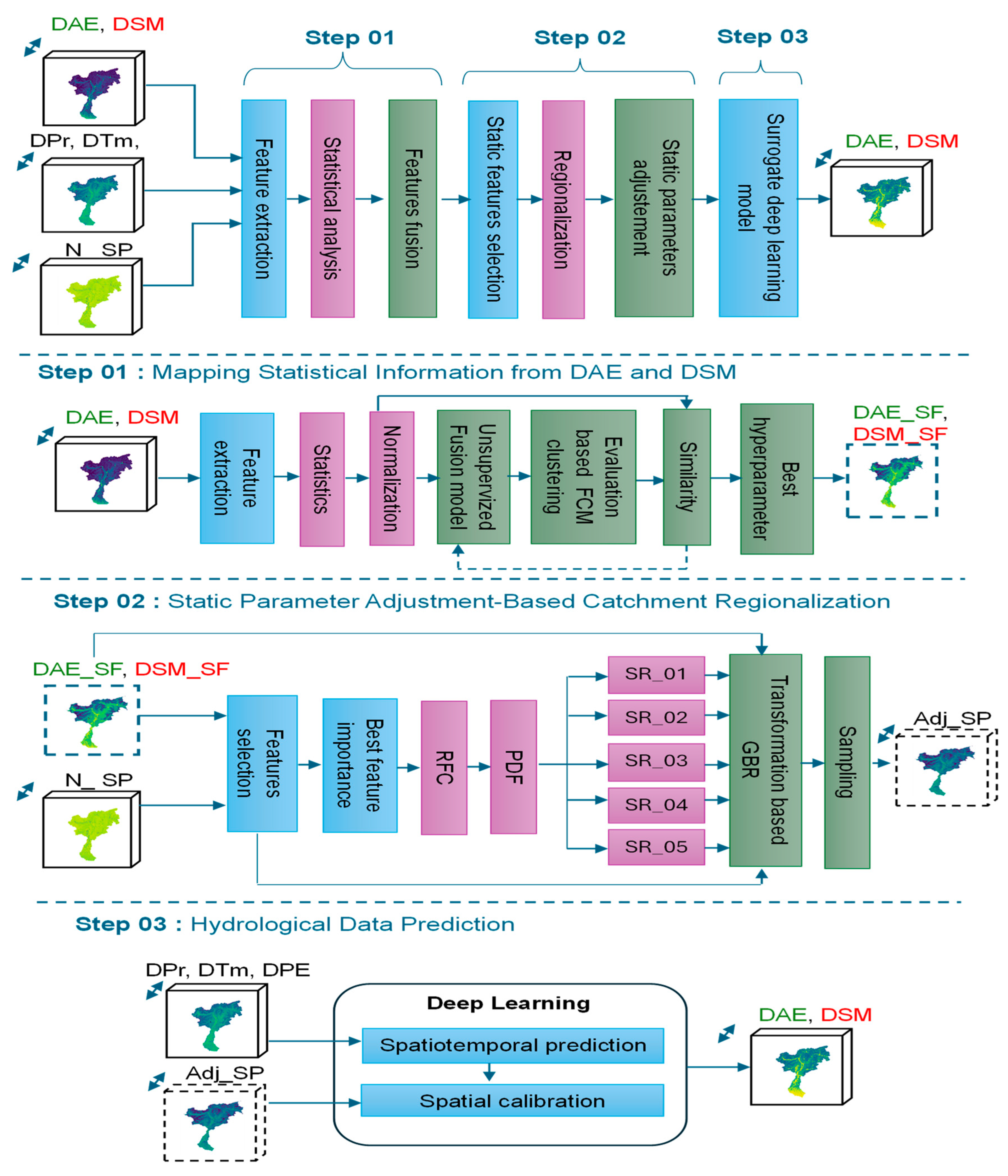
The proposed SDL model architecture aims to predict hydrological parameters, with a particular focus on DAE and DSM. Its primary goal is to simplify the complexity of traditional data-driven models while enhancing the interpretability of the resulting predictions across spatiotemporal scales, as illustrated in Figure 2. In this study, target outputs generated by a physical hydrological model are used to train the SDL architecture, incorporating climate inputs, such as precipitation, temperature, and potential evapotranspiration.

To support calibration, a set of static parameters describing geophysical characteristics of the catchment is integrated into the model framework. This integration addresses challenges related to inconsistencies and heterogeneity in the spatial distribution of static parameters compared to hydrological variables, which can introduce biases across the region. Consequently, the framework focuses on improving the quality and homogeneity of static parameters to enhance the SDL model’s spatiotemporal prediction accuracy, enabling efficient training with relatively few epochs. The proposed framework is structured into three interrelated steps, each aimed at improving the calibration and predictive performance of the SDL hydrological model.

4.1. Mapping Statistical Information from DAE and DSM

This step begins with extracting dynamic datasets for key hydrological parameters, such as DAE and DSM. For each spatial location, a range of statistical indicators—including measures of variability, distribution, and density—are computed to effectively capture the temporal characteristics of these dynamic features. These indicators are then normalized to ensure consistency and comparability across different scales and units. Following normalization, unsupervised learning methods are applied to integrate and reduce the dimensionality of the features, thereby uncovering the essential spatial patterns.

To verify that the dimensionality reduction preserves important spatial variability, the similarity between clustering results based on the fused features and those derived from the full set of statistics is evaluated using the Adjusted Rand Index (ARI). Multiple models are explored and retrained during this fusion process to optimize hyperparameters, ensuring the best possible representation of the spatiotemporal statistical characteristics of DAE and DSM within a spatial latent space.

4.2. Static Parameter Adjustment-Based Catchment Regionalization

After confirming the effectiveness of the fusion, the mapped features are used to guide the selection of relevant static parameters by analyzing both the correlation and the similarity in distribution between each parameter and the fused DAE and DSM features. This analysis employs the correlation coefficient (R) and the Kolmogorov–Smirnov (KS) statistical test. These metrics support the establishment of an optimal selection criterion, targeting correlation values greater than 0.5 and KS statistics less than 0.5. These thresholds are chosen to capture meaningful relationships between static parameters and fused dynamic features, considering the complex and non-linear nature of the data.

It is important to note that a high correlation alone does not guarantee consistent spatial alignment between a static parameter and the fused DAE and DSM features across the entire region. This limitation is addressed by comparing the similarity of their distributions through the KS test. The threshold of 0.5 for the Kolmogorov–Smirnov (KS) statistic is empirically proposed based on the normalization of cumulative distribution functions (CDFs) within the range [0, 1], enabling consistent comparisons across different parameters. The KS statistic measures the maximum absolute difference between two empirical CDFs and varies between 0 and 1. A threshold value of 0.5 corresponds to a 50% maximum divergence between two normalized distributions, making it a practical criterion for classifying them as similar or dissimilar. Although not universally fixed, this threshold has been used in several studies as a heuristic for assessing the separability of distributions in normalized spaces [56,57].

Parameter calibration adjustment based on catchment regionalization involves defining transformation models within each identified cluster using Gradient Boosting Regression (GBR). The process begins by identifying the most important static parameters, which serve as the basis for subdividing the catchments. This regionalization is performed using the Random Forest Classifier (RFC) [58], grouping catchments into subregions that exhibit similar statistical characteristics. To describe and distinguish each subregion, Probability Density Function (PDF) plots are generated. These plots provide theoretical insight into the distribution of selected static parameters within each cluster, facilitating the reproducibility of the transformation method across other subregions. Within each subregion, a GBR model is trained using the selected static parameter as the input feature and the fused representation of DAE and DSM as the target variable. This regression-based transformation aligns the static parameter distributions with the dynamic behavior captured by the fusion feature, enhancing consistency between static and dynamic inputs and improving the surrogate model’s learning capacity. Finally, the adjusted parameters within each subregion are sampled and propagated, ensuring homogeneous and spatially coherent parameters throughout the whole region.

4.3. Hydrological Data Prediction

This step builds upon the outputs of the earlier preprocessing and transformation steps by utilizing a harmonized set of inputs—comprising dynamic climate variables and adjusted static parameters. These inputs are specifically prepared to reflect spatiotemporal coherence and internal consistency, ensuring that the surrogate model receives high-quality training data. At this stage, a DL model based on an RNN architecture is employed to simulate hydrological processes across the spatial and temporal scale. By leveraging the improved input structure, the model captures complex non-linear interactions between climate forcings and static catchment characteristics, thereby enhancing the accuracy and spatially generalizability of hydrological predictions. Crucially, the integration of transformed static parameters—aligned with the fused dynamic feature space—enhances the model’s calibration performance and reduces prediction biases. These improvements are particularly significant to account for seasonal variations and changes in climate drivers, which often introduce inconsistencies in conventional modeling approaches. The calibrated surrogate model, therefore, not only replicates the outputs of more computationally intensive hydrological models but also provides scalable, efficient predictions suitable for large-scale catchment applications.

5. Results

This section presents the results of enhancing parameter calibration for SDL hydrological models, incorporating both DAE and DSM. The process starts with the integration of spatiotemporal information from WFLOW using unsupervised model fusion, followed by the evaluation of static data transformation through catchment regionalization. The primary objective is to assess the effectiveness of the proposed approach in improving model performance across various SDL model architectures, using a fixed number of training epochs. Models such as LSTM, GRU, TCN, and ConvLSTM are evaluated. Both qualitative and quantitative analyses are performed, employing multiple scales, such as mean daily data to assess the spatial scale and 3D residual data plots along with regression plots from different sites within the catchment to evaluate the temporal scale.

5.1. Data Exploration

The application of DL models for hydrological prediction largely depends on comprehensive data preprocessing and partitioning. These steps are critical to ensure that models are trained on high-quality data and can generalize effectively to unseen scenarios, thereby enhancing the prediction accuracy and reliability. The use of geocubic data frames provides an advanced and robust framework for analyzing spatiotemporal data distributions.

This structured format encapsulates multidimensional arrays, facilitating the integration of various hydroclimatic variables, such as precipitation, temperature, and potential evapotranspiration, which are pivotal for assessing their distribution patterns across spatiotemporal scales. Effective data partitioning is essential for training and evaluating hydrological models to ensure reliable performance and generalizability across different spatial and temporal scales. In this study, we used random splitting provided by the scikit-learn library in Python to divide the spatiotemporal data dataset from 2018–2022 into 60:40 ratio for training and testing. To further enhance the quality of the split and reduce the risk of overfitting between the training and testing phases, we applied a uniform sampling approach based on density differences. This method allowed us to better capture the variability within the data across the full spatiotemporal extent. This is essential for analyzing various steps proposed in the surrogate hydrological model, including data transformation and an accuracy assessment of DL models. Figure 3 depicts the spatial split of data used for the proposed SDL model, along with a comparative density analysis using Kernel Density Estimation (KDE) maps and an evaluation of density differences based on uniform spatial sampling. Furthermore, a descriptive analysis of both the training and testing sets is provided, using normalized input and target values, as depicted in box plots and density curves. The results show that the selected pixels are uniformly distributed in most parts of the study area, with higher densities concentrated in the middle and southern part of the catchment. However, the uniformity analysis for the smaller samples reveals notable density differences between the training and testing subsets, with values ranging between 0.6 and 1 in most cases (see Figure 3A).

The data splitting technique is well-suited for hyperparameter tuning and for evaluating the performance of SDL models across spatiotemporal scales. Figure 3 provides additional insights through box plots and density curves, highlighting the distribution and variability of target and input data for both training and testing areas. This analysis compares the patterns of each feature, including the daily actual evapotranspiration (DAE), soil moisture (DSM), precipitation (DPr), temperature (DTm), potential evapotranspiration (DEp), and static parameters (SP), across spatiotemporal scales.

A notable disparity is observed between the training and testing datasets, particularly in DEp, DPr, and DAE, where non-stationary behaviors are present during training and skewness toward higher values is evident. In contrast, static parameters exhibit a heterogeneous distribution, especially in the testing phase. Meanwhile, daily soil moisture and temperature maintain a more consistent stationarity across both phases, as indicated by similar coefficient of variation (Cv) values of 0.51 and 0.50 for soil moisture and 0.33 and 0.32 for temperature. These observations provide valuable insights into the distribution patterns of hydrological processes, underscoring the complexity and challenges in accurately estimating DAE and DSM.

5.2. Spatio-Temporal Information Fusion for Wflow Parameters

The spatiotemporal analysis of hydrological parameters raises a fundamental research question on how complex multidimensional data can be effectively represented to comprehend pattern distribution and density across an entire region. To address this, our study presents several fusion models designed to reduce dimensionality and combine diverse information from DAE and DSM. A range of statistical metrics is thoroughly evaluated and incorporated during preprocessing to capture the intricate details within the spatiotemporal context, enabling the integration of this information into a single feature.

A comprehensive statistical overview of hydrological parameters across the Adige region is presented, focusing on variability (Cv), data distribution (mean, median, Q1, and Q3), density (skewness and kurtosis), and pattern tendencies (autocorrelation). Concurrently, diverse models are employed, categorized into feature reduction approaches, such as t-SNE and UMAP, and encoder learning models, including Autoencoder, Variational Autoencoder (VAE), and Deep Belief Network (DBN). Leveraging these different architectures helps in identifying an optimal model for accurately fusing the spatiotemporal information from DAE and DSM. This approach enhances our ability to accurately identify and interpret the distribution and density patterns of hydrological parameters across the study area. Evaluating the performance of unsupervised learning models presents considerable challenges, primarily due to the lack of regressor labels for the comparison. Consequently, their performance is assessed based on the structure and characteristics of the data that they reveal. One method used in this analysis to assess the accuracy of unsupervised fusion models involves comparing the similarity of data distributions across clusters obtained through the application of the FCM model, using Adjusted Rand Index (ARI) scores. This evaluation compares clusters generated from the full set of statistical features with those derived from the fused feature.

Figure 4 presents statistical assessment maps of DAE and DSM using various indices. Normalized data were employed to facilitate the comparative analysis of pattern distributions between DAE and DSM. The comparison with mean values highlights spatial homogeneity across the region. These indices provide valuable insights into both the temporal and spatial characteristics of the data. The results demonstrate a consistent variability around the mean values for DAE, with values ranging from 0.2 to 0.6. The maps reveal a high distribution of mean values for DSM compared to DAE, varying from 0.1 to 0.9. The density analysis, based on skewness parameters, indicates that DSM shows low similarity to a log-normal distribution compared to DAE, with skewness values exceeding 0.9. Conversely, the kurtosis analysis for DSM indicates a null value across the entire basin, suggesting that the peak of the distribution is flatter than that of a normal distribution, with less concentration of data around the mean.

Moreover, the autocorrelation plots reveal a very low fit of temporal data for both parameters, particularly in the northern part of the catchment. This indicates a lack of a strong temporal correlation in the data for both DAE and DSM, highlighting areas where the model may need improvement. Overall, these statistical assessments provide a comprehensive evaluation of the performance and characteristics of the unsupervised learning models, offering insights into their effectiveness in capturing the underlying patterns in the data.

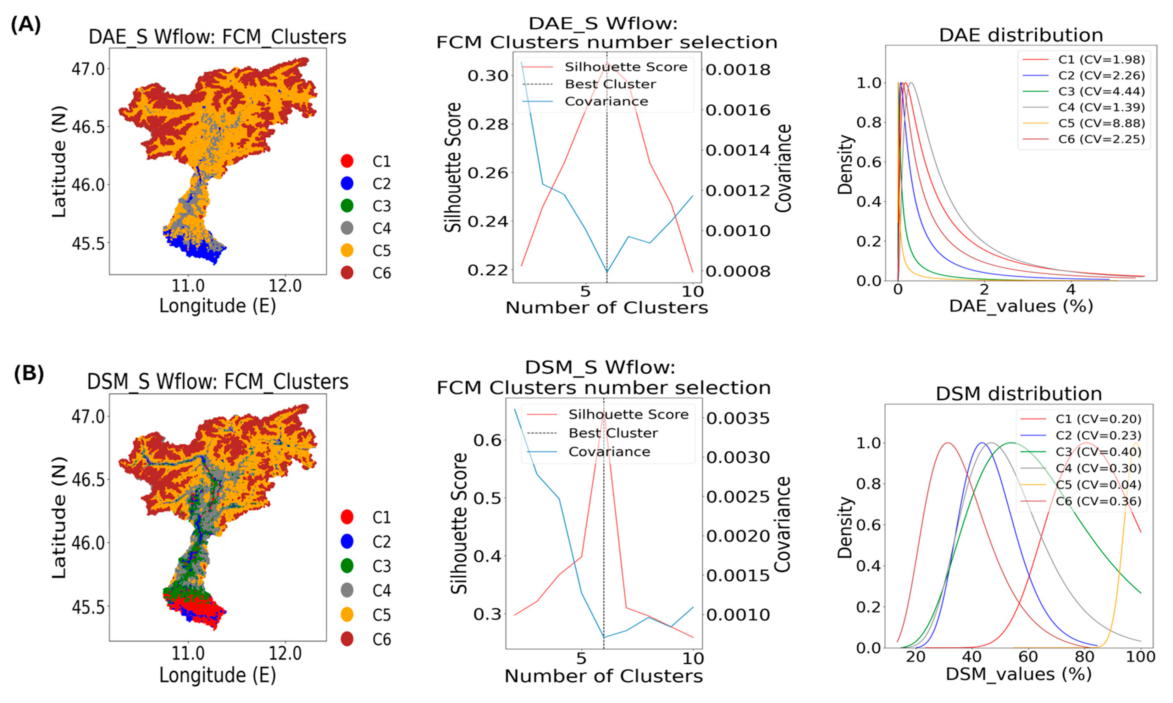
Figure 5 presents the results of applying FCM clustering using the proposed statistical indices for both DAE and DSM. The selection of the optimal number of clusters was based on the silhouette score and covariance index. An optimal clustering configuration was identified by maximizing the silhouette score while minimizing the covariance value. According to the results, dividing the basin into six clusters provided the best performance for both DAE and DSM, yielding the highest silhouette scores and the lowest covariance values. Additionally, the density analysis revealed significant differences between the clusters derived from the DSM and those from the DAE. While the data for both models exhibited a range between 0 and 5 mm, the density distributions for each cluster were slightly skewed. This suggests a disparity in the underlying data distributions captured by the DAE and DSM, despite the shared range of values.

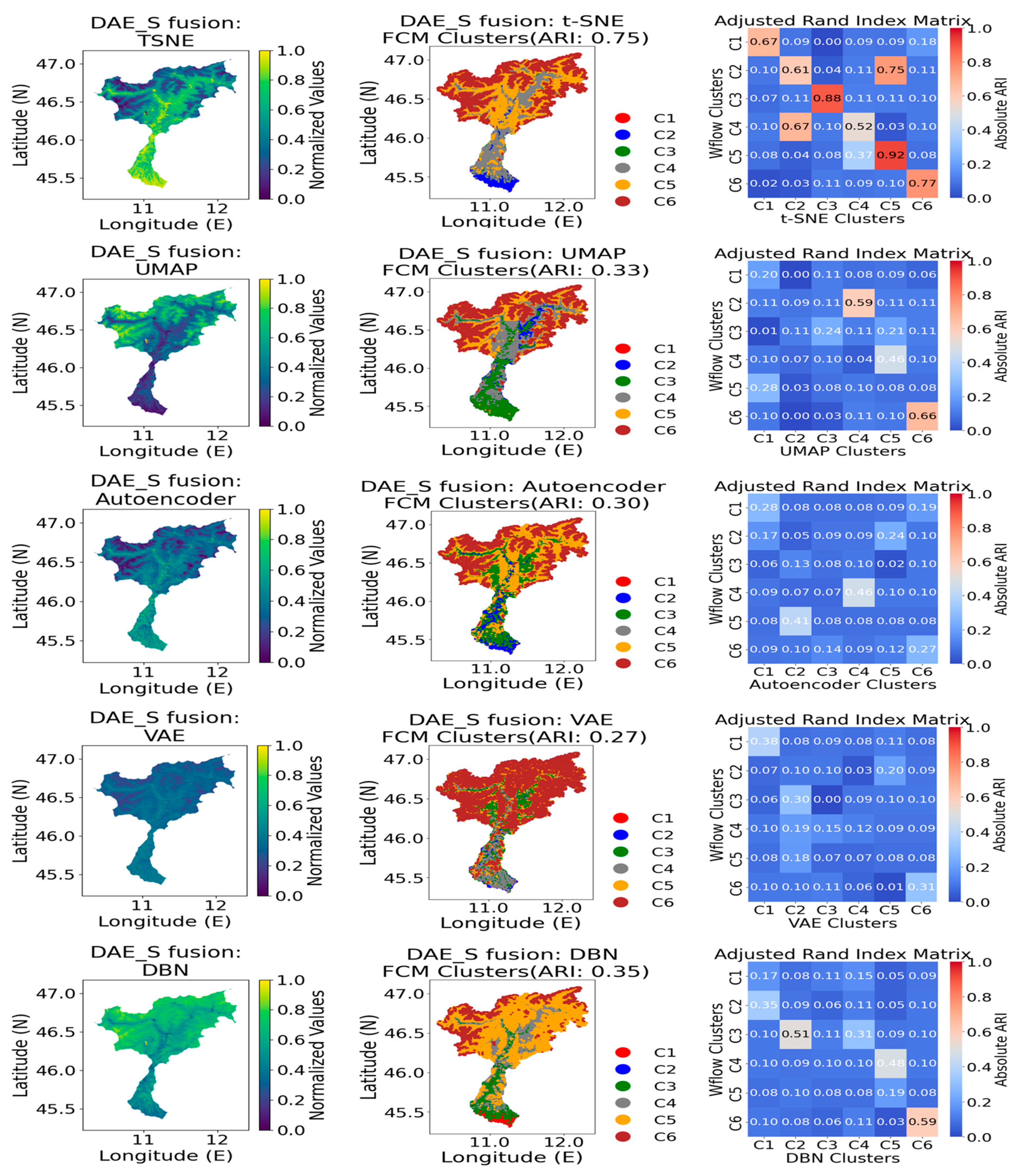
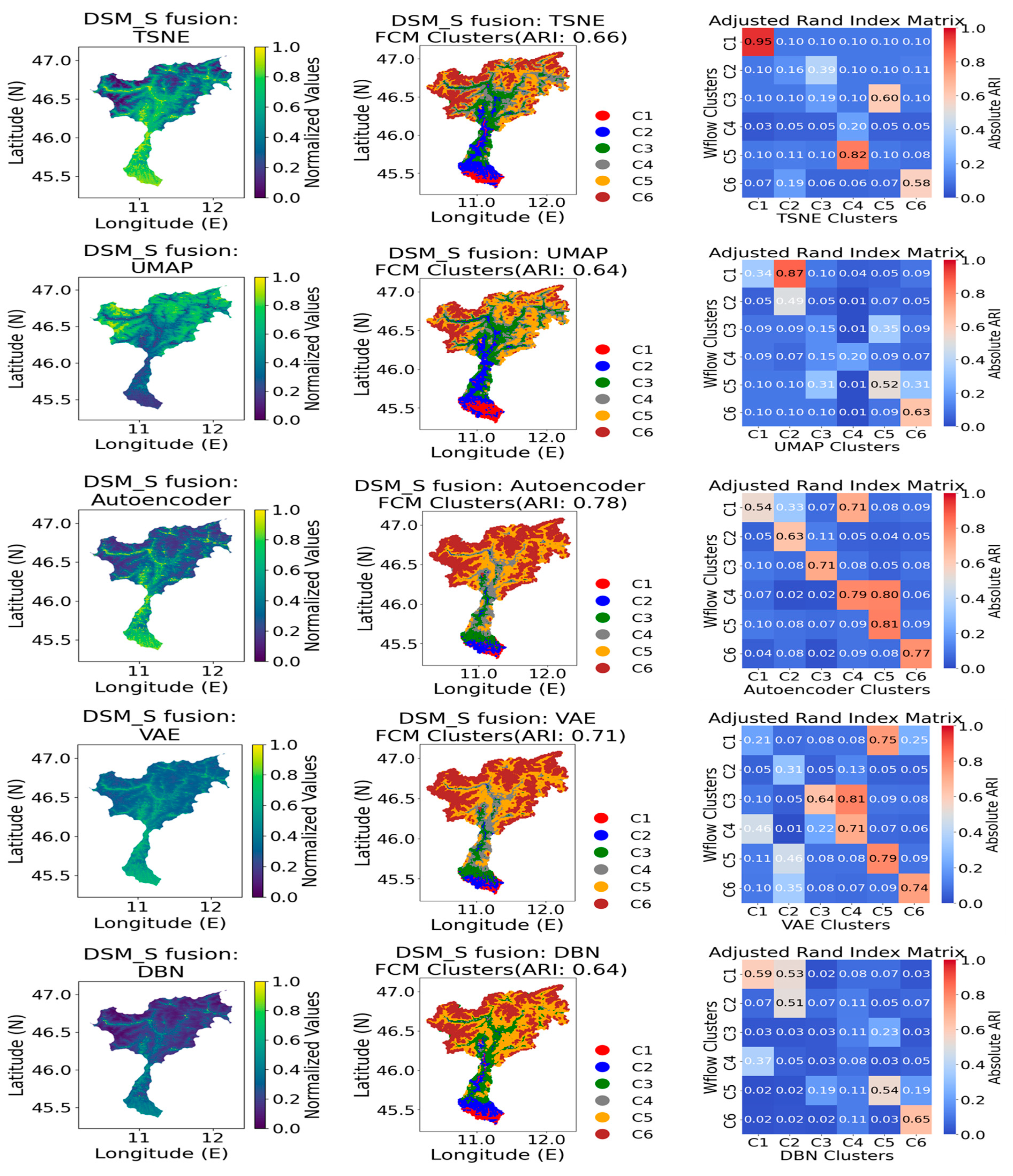
The differing density patterns indicate that while both models are effective in clustering, they capture and represent the data’s statistical properties in distinct ways. This analysis underscores the importance of evaluating both similarity metrics and density distributions to gain a comprehensive understanding of the clustering performance and the data’s intrinsic characteristics. A comparative evaluation of fused statistical data for both DAE and DSM, using various unsupervised learning models, was conducted through FCM clustering analysis (see Figure 6 and Figure 7). The results reveal a strong alignment between clusters obtained from the complete set of statistical features and those produced through t-SNE fusion, particularly for DAE. This alignment is quantitatively measured based on ARI heatmap values ranging from 0.52 to 0.92 (see Figure 6), underscoring the robustness of the fusion approach in effectively capturing spatiotemporal pattern distributions as a unified feature across the basin. Furthermore, the integration of DSM statistical data highlights the efficacy of the Autoencoder model, demonstrating enhanced cluster alignment and its capability to represent non-stationary DSM patterns across the region, with an ARI value of 0.78 (see Figure 7). This is accomplished by generating a new dataset that incorporates mean and variance parameters as estimators. Although the Variational Autoencoders (VAEs) employed in this study assumed a continuous latent space with a specific distribution, typically Gaussian, their application resulted in some information loss, particularly for clusters 1 and 2.

Nevertheless, VAEs performed effectively for the remaining DSM clusters, positioning them as a viable alternative to the Deep Belief Network (DBN). This last one excels in capturing pattern distributions across several clusters, including the 1st, 2nd, 5th, and 6th. Both models, VAEs and DBNs, can complementarity fuse DSM-related information, offering a comprehensive approach to data integration and analysis. This integrated approach enhances the understanding by capturing nuances in density, variability, and distribution patterns of both DSM and DAE, which are essential for robust hydrological modeling and resource-management strategies.

5.3. Static Feature Selection

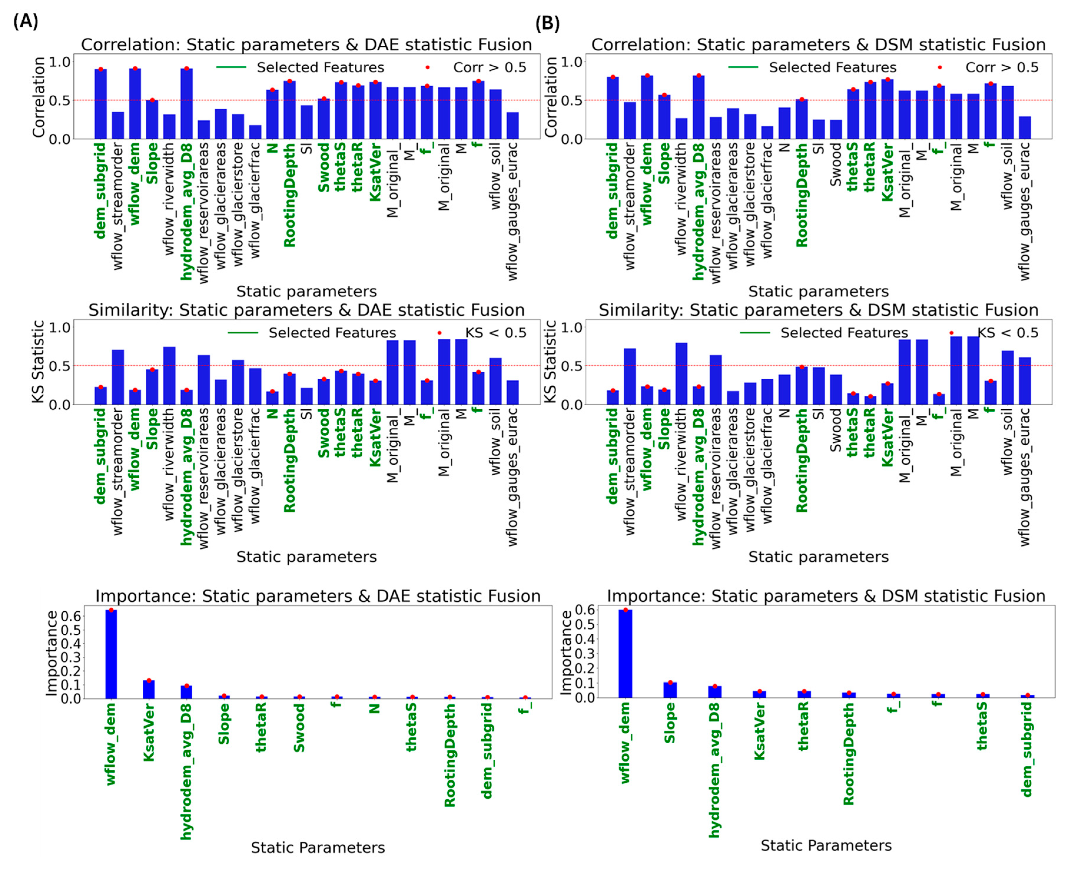
Figure 8 presents the feature selection analysis to identify parameters used for SDL model calibration in the Adige catchment. The results show a strong fit for 12 out of 25 features with DAE and 10 out of 25 with DSM. Notably, subgrid_dem, Wflow_dem, and hydrodem_avg_D8 exhibited correlation values exceeding 0.8 and skewness (Ks) below 0.25, indicating strong fit with ground truth data. These features are reliable for model calibration due to their consistency across statistical and density-based metrics. Moreover, parameters such as the Rooting Depth, Swood, ThetaS, ThetaR, Ksatver, f-, and F demonstrated strong alignment with both DAE and DSM, thereby enhancing the accuracy and robustness of the SDL. On the other hand, the results identified features that fail to improve the SDL model’s performance and may adversely affect its accuracy. Specifically, the N and Swood features introduce bias when compared to DSM, suggesting inconsistency in capturing the underlying patterns across the entire region. Additionally, Figure 8 offers valuable insight into the contributions of geophysical parameters to the SDL model calibration. The features selected through this process enhance our understanding of how the static parameters improve the accuracy and robustness of the modeling outcomes by leveraging the degree of fit with DAE and DSM. Figure 8 also illustrates the importance of each selected feature for both DAE and DSM, highlighting that Wflow_dem contributes significantly, with an important score of 60% compared to the other features in both cases. Additionally, Ksatver exhibits a notably higher importance in the case of DAE compared to DSM, whereas the Slope parameter demonstrates a greater contribution in DSM than in DAE.

5.4. Catchment Regionalization

In this section, a supervised approach for catchment regionalization is introduced, using geophysical information from the target catchment. The choice of input feature should demonstrate consistent alignment with both DAE and DSM, providing information about elevation across the entire region. This feature is crucial for characterizing the landscape and offers valuable insights to subdivide the target catchment into homogenous subregions. The selection of Wflow_dem in this study was based on its strong alignment with the feature fusion of Wflow parameters. Furthermore, it significantly contributes to the RFC, acting as a main key for data classification with both components, outperforming the other static parameters (see Figure 8). Developing a method for region classification is challenging due to the nonlinear variation in elevation across the region.

To address these challenges, the Random Forest classifier (RFC) employs an ensemble approach by constructing multiple decision trees during training and determining the mode of their class predictions. This method effectively captures the complexities inherent in nonlinear data relationships. To enhance the reproducibility of the proposed methodology for broader applications, Kernel density estimation (KDE) was integrated to characterize the distribution of the Wflow_dem parameter within each subregion. 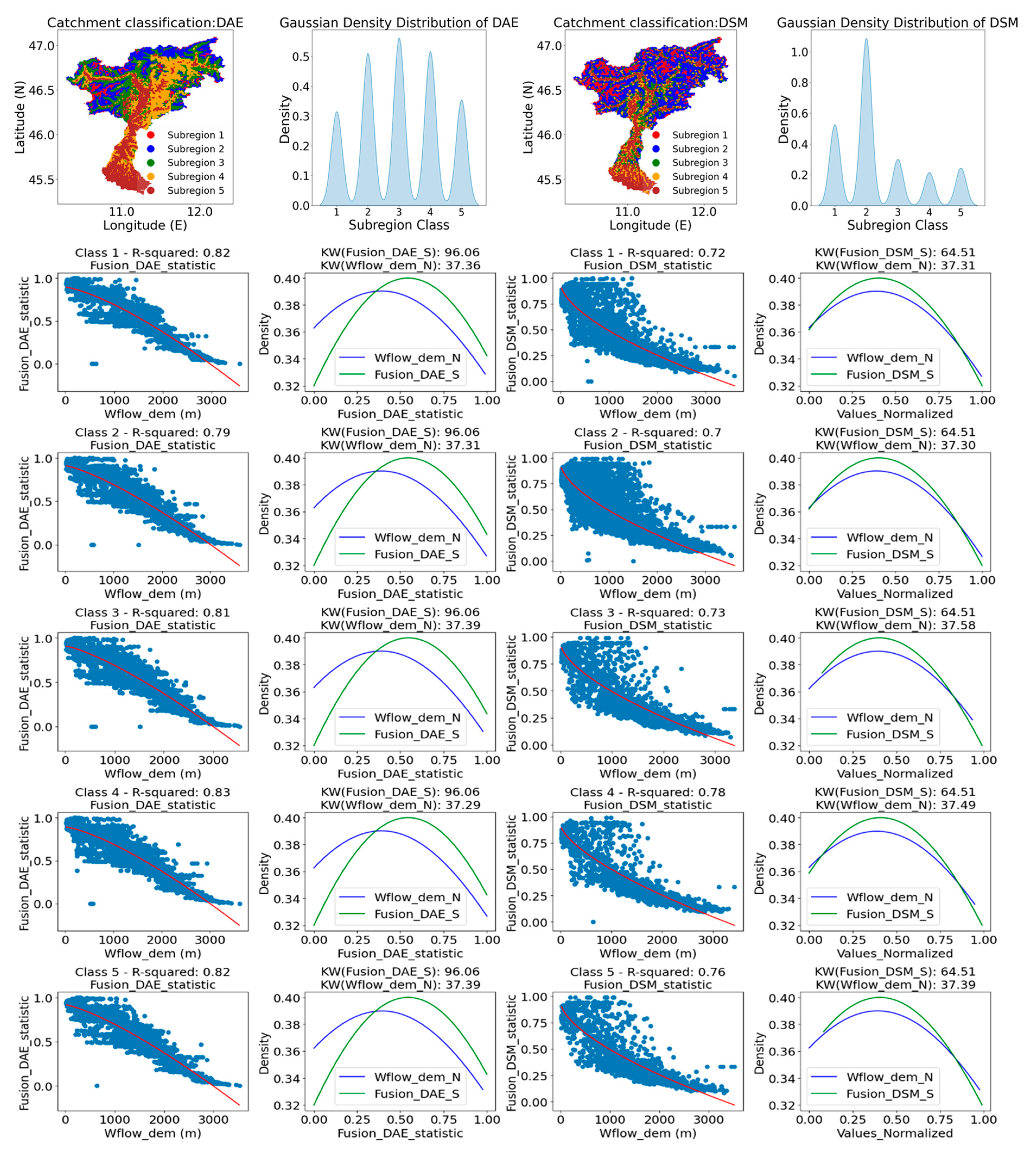Figure 9 presents the outcomes of applying RFC for the subregion classification of daily actual evapotranspiration (DAE) and daily soil moisture (DSM) within the Adige catchment.

The Wflow_dem parameter exhibits substantial correlations, ranging from 0.79 to 0.83 for DAE and from 0.70 to 0.78 for DSM across various subregions. Additionally, KDE analyses reveal consistent spatial patterns when comparing Wflow_dem with statistical fusion data for both DAE and DSM. Partitioning the region into five subregions highlights distinct density variations represented by Gaussian curves. Notable concentrations are observed in classes 2, 3, and 4 for DAE and class 2 for DSM, underscoring the importance of subregion-specific patterns for an accurate hydrological characterization.

These findings emphasize the effectiveness of RFC in delineating meaningful subregions based on hydrological parameters, thereby facilitating a deeper understanding of the landscape heterogeneity and supporting spatiotemporal analyses. Moreover, the integration of KDE distinguishes variations between subregions and serves as a theoretical density benchmark for comparisons with Wflow_dem data from other regions. This approach ensures a comprehensive characterization of regional hydrological dynamics and enhances the applicability of the findings beyond the Adige catchment. The demonstrated methodology holds potential for applications in similar geographical contexts, offering valuable insights for resource management and environmental planning.

5.5. Calibrated Parameter Transformation

In this section, the transformed approach is implemented using the Gradient Boosting Regression (GBR) model to adjust selected parameters based on the fitted density of statistical fusion features for both DAE and DSM. The methodology involves training the GBR model to iteratively optimize predictions by combining multiple weak learners, thereby capturing complex relationships within the data. The model refines the estimation of statistical fusion features by minimizing prediction errors in successive stages, making it well-suited for enhancing parameter adjustments. This approach ensures the accurate transformation of the selected parameters, ultimately improving the robustness of SDL calibration parameters for both DAE and DSM. Once the model is fitted, each static parameter data point is assigned probabilities corresponding to each gradient component of the GBR model. For transformation, data points are mapped using normalized values based on their posterior probabilities or maximum likelihood estimates, ensuring consistency with the density characteristics of the original dataset. Figure 10 illustrates the application of the GBR-transformed model across the first subregion, applied to the selected static parameters identified for DAE and DSM. The results present Gaussian curves and regression plots, illustrating the static parameters both before and after transformation. These are compared to the ground truth density, highlighting the effectiveness of the transformation in aligning the parameters with the expected density characteristics. Figure 10 also shows a notable improvement in the quality of static parameters following the transformation. Three variables were selected based on their differing contributions to the daily actual evapotranspiration (DAE), using DAE statistical fusion feature (DAE_SF), to evaluate the method’s capacity to improve parameter accuracy under varying relevance conditions. The transformation process led to substantial gains in both correlation and density alignment with the DAE_SF feature, with R² values exceeding 0.7 and Kolmogorov–Smirnov (KS) statistics remaining below 0.12. These outcomes highlight the method’s effectiveness in optimizing static parameter representation for the SDL model calibration. Additionally, the same approach was applied using the daily soil moisture statistical fusion feature (DSM_SF) within the same subregion. The results demonstrate marked improvement in parameter alignment, particularly for the KsatVer parameter, where the correlation increases from 0.14 to 0.65 following the GBR transformation (Figure 10B).

This enhancement is further supported by the density plots, where the KS value decreased to 0.25, indicating greater similarity with the DSM distribution. These findings confirm the robustness of the GBR model in refining parameter calibration and improving the predictive capacity of the SDL framework.

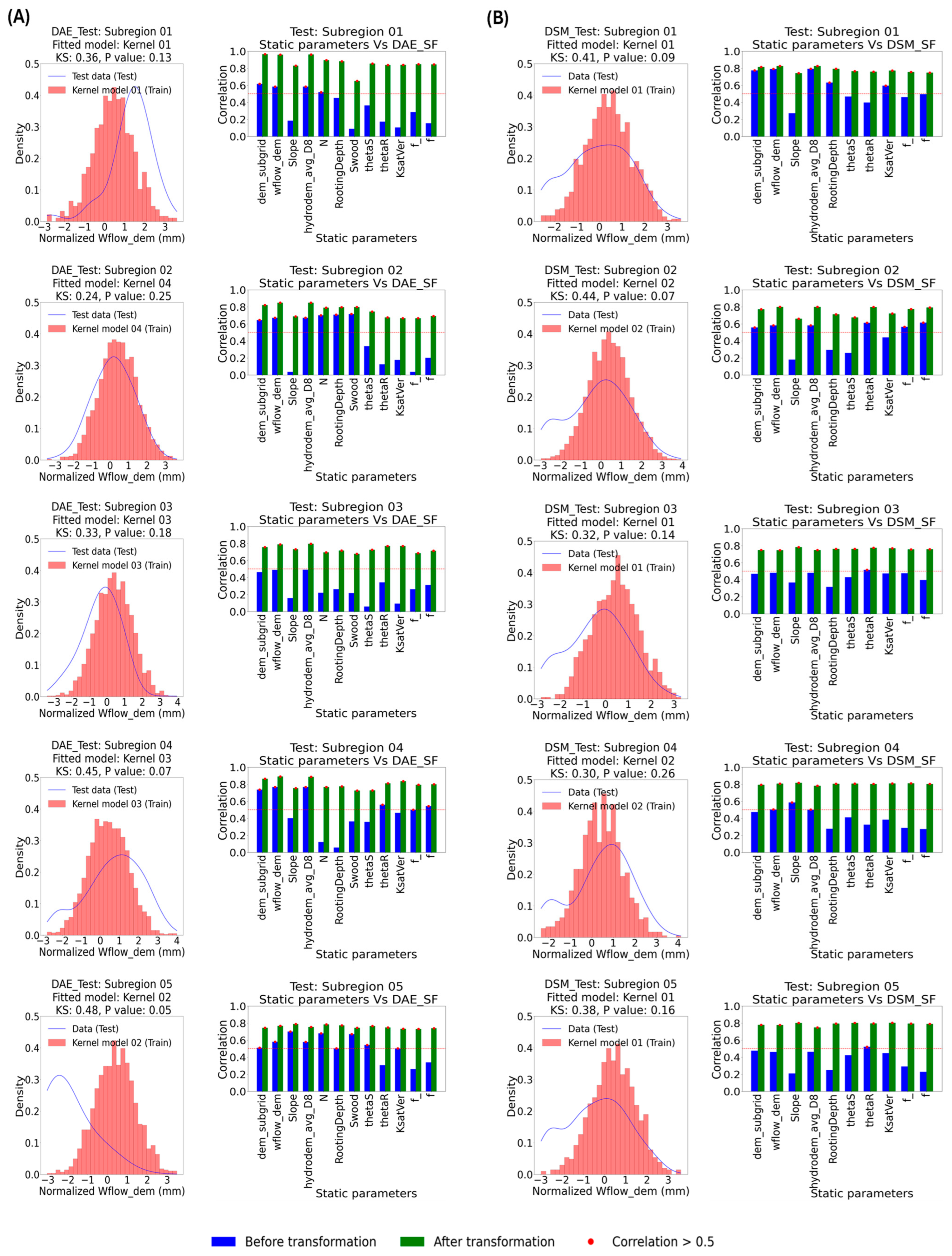
Figure 11 presents the results of evaluating the proposed data transformation approach developed during the training phase for each subregion. Classification of the testing area is performed using the RFC model generated during training.

Kernel Density Estimation (KDE) is applied to compare the resulting classes with the theoretical density distributions of the corresponding subregions, utilizing the Kolmogorov–Smirnov (KS) test for static parameters. In each subregion, the effectiveness of the GBR transformation method, established during the training phase, is assessed by applying it to the static parameters of the test area. Figure 11 provides additional insights into the quality of these transformed static parameters, demonstrating the performance of the RFC_GBR model. This comparison is conducted against the fusion features proposed for DAE and DSM. The classification of the test region into distinct subregions helps explain the reproducibility of the transformed models for other applications. The results show that four transformed models were selected, corresponding to subregions 1, 2, 3, and 4, based on their similarity to the Kernel theoretical density obtained during the DAE training phase. Moreover, parameters proposed for SDL model calibration in the case of DSM across all subregions were adjusted using the models proposed for subregions 1 and 4 during the training phase (refer to Figure 11B). This analysis demonstrates the effectiveness of the GBR approach in refining parameter calibrations for both cases, with significant improvements observed, evidenced by correlation values exceeding 0.5 in all cases. This improvement is particularly evident for the N, Rooting-Depth, and Swood parameters in the DAE case and for the Slope, theatS, and theataR parameters in the DSM case. Furthermore, the histogram plots highlight the stability and consistency of the adjusted parameter alignment with the ground truth, reinforcing the robustness of the SDL model calibration across the entire region.

6. Discussions

To rigorously assess the effectiveness of the transformed calibration approach across multiple SDL architectures—including LSTM, GRU, TCN, and ConvLSTM—we propose a scenario where the training process is fixed to 50 epochs for each model. This constraint is intentionally applied to provide a consistent and controlled framework that better visualizes the biases present in the data and clearly highlights the improvements brought by the use of adjusted parameter calibration. By limiting the training duration, this scenario ensures a fair and standardized comparison, allowing us to evaluate the impact of the calibrated parameters on the SDL models. Moreover, it demonstrates that high-quality hydrological predictions can be achieved without extensive training, offering a more computationally efficient pathway for large-scale spatiotemporal modeling.

Figure 12 and Figure 13 present the results of predicting DAE and DSM using SDL models trained with selected static features (SFs), both before and after the transformation process. Four SDL architectures were tested to compare their performance in predicting these hydrological variables. The evaluation includes training loss over 50 epochs and compares the predicted values to the ground truth using boxplots and density plots. These results illustrate how feature transformation improves the prediction accuracy and demonstrates the effectiveness of each model architecture. The findings indicate that ConvLSTM demonstrated very high performance in predicting both DAE and DSM before transformation of the selected features. Furthermore, an improvement in performance was observed after integrating the transformed parameters into the SDL model for calibration.

This resulted in consistent accuracy across all models, due to the use of high-quality calibration parameters. The results provide valuable insights for hydrological modeling, suggesting that simpler models can achieve competitive accuracy, thereby reducing the need for more complex models such as ConvLSTM.

Figure 14 illustrates a spatiotemporal descriptive analysis of SDL model performance for predicting DAE and DSM, using static parameters for model calibration before and after transformation (TF). The evaluation assesses DAE results using maps for humid and dry periods, followed by density curves comparing predicted data to the Wflow ground truth on a daily mean scale. This approach effectively captures the spatial performance of the SDL model accuracy across the entire region. Additionally, splitting the data into wet and dry periods helps in identifying model biases and evaluating the improvements gained by integrating the transformed parameters to enhance SDL model accuracy.

The analysis focuses on LSTM and GRU models to evaluate the extent to which the adjusted calibration parameters enhance the performance for the simplest model architecture, which is the primary objective of this study. The results demonstrate performance improvements of 20% and 28% for LSTM and GRU, respectively. Particularly, when predicting DAE during humid periods, this is reflected in R² scores of 0.94 and 0.92, respectively (see Figure 14A). These improvements are further supported by a high similarity of density with the target data, given by KS values of 0.04 for LSTM and 0.06 for GRU. 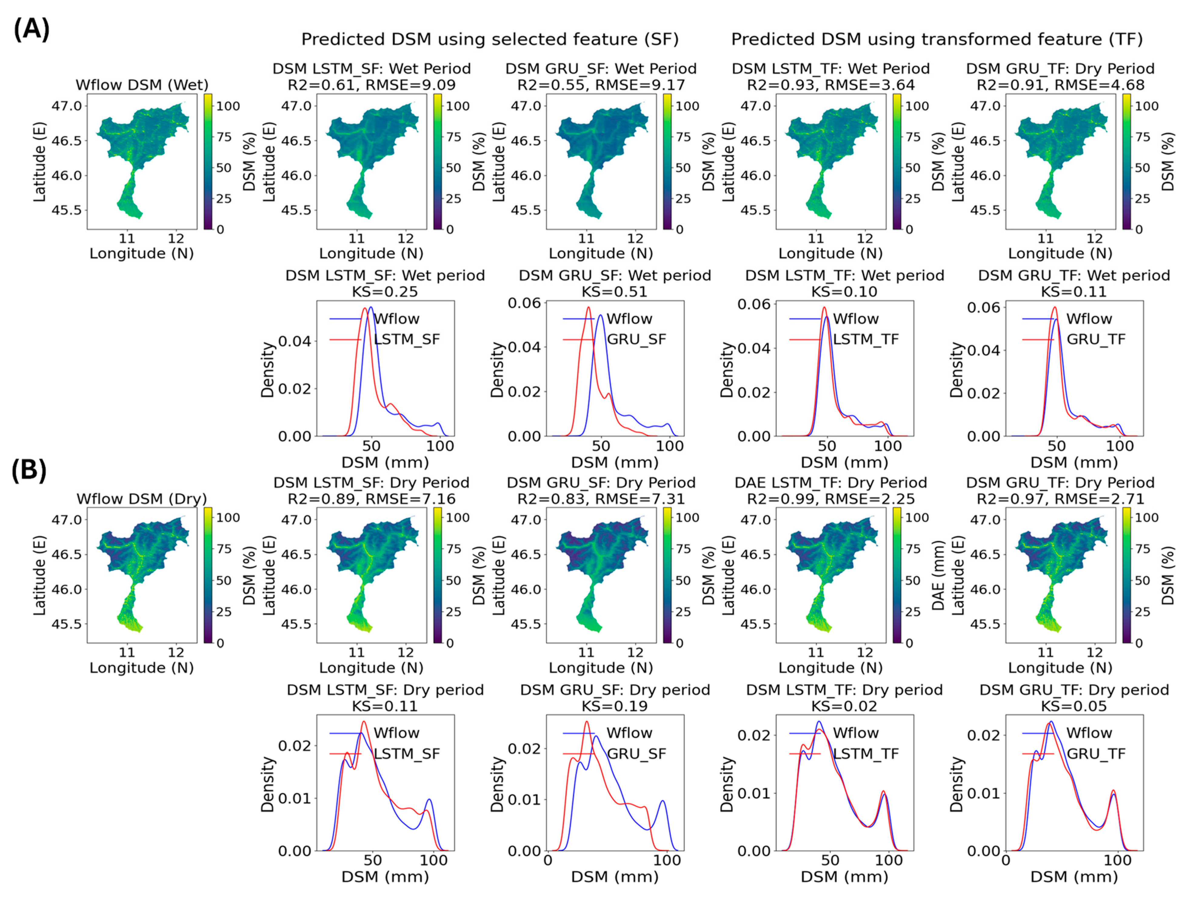A similar comparison during the dry period reveals further performance gains for both models when using adjusted parameters, with R² scores of 0.98 and 0.96 with LSRM and GRU, respectively. In this case, the transformed parameters lead to a remarkable 42% improvement, particularly for the GRU. These findings highlight the effectiveness of the proposed parameter calibration transformation in enhancing SDL model accuracy while maintaining relatively simple model architectures. When estimating DSM using adjusted parameters for SDL model calibration, substantial improvements in result quality are achieved with both LSTM and GRU models, even when using a limited number of epochs. As shown in Figure 15, model accuracy increases by 32% and 36% during the wet period for LSTM and GRU, respectively. Additionally, the maps demonstrate that employing transformed features enhances the ability to capture finer details of DAE across the catchment, particularly for maximum values extending up to 100 mm. A similar trend is observed when estimating DSM during the dry period using the same calibrated parameters, with R² values of 0.99 and 0.97 for LSTM and GRU, respectively.

The high performance of the SDL models during this period is further corroborated by the density curves, yielding similarity scores of 0.02 for LSTM and 0.05 for GRU. These results emphasize the effectiveness of the transformed features in improving model accuracy across different periods. Figure 16 presents absolute residual analysis plots comparing the Wflow ground truth data with predicted DAE and DSM using LSTM and GRU models, focusing on a daily timescale between 2018 and 2022. The plots illustrate two processing scenarios based on the selected features (SFs) and transformed features (TFs) used for model calibration. Additionally, the results are divided into training and testing phases, with a three-year training period (2018 to 2020) and a two-year testing period (2021 to 2022). In this step, a comprehensive analysis was conducted using 3D plots, where the x-axis represents the catchment pixels, the y-axis represents the daily timeline, and the z-axis represents absolute residual values. Overall, the results indicate a significant improvement in prediction quality when transformed parameters are applied using the RFC_GBR approach, underscoring the effectiveness of the proposed technique-based regionalization in enhancing SDL model performance for DAE and DSM assessments. Moreover, LSTM and GRU models demonstrate superior performance in estimating DAE compared to DSM, as illustrated in Figure 16. The integration of transformed parameters leads to a substantial reduction in bias, emphasizing the impact of parameter calibration on model accuracy. During the training phase, some pixels exhibit residuals between 0.6 mm and 1 mm when using the selected parameters. However, with the transformed parameters, both models show improvements, with residuals consistently reduced to approximately 0.2 mm across the region.

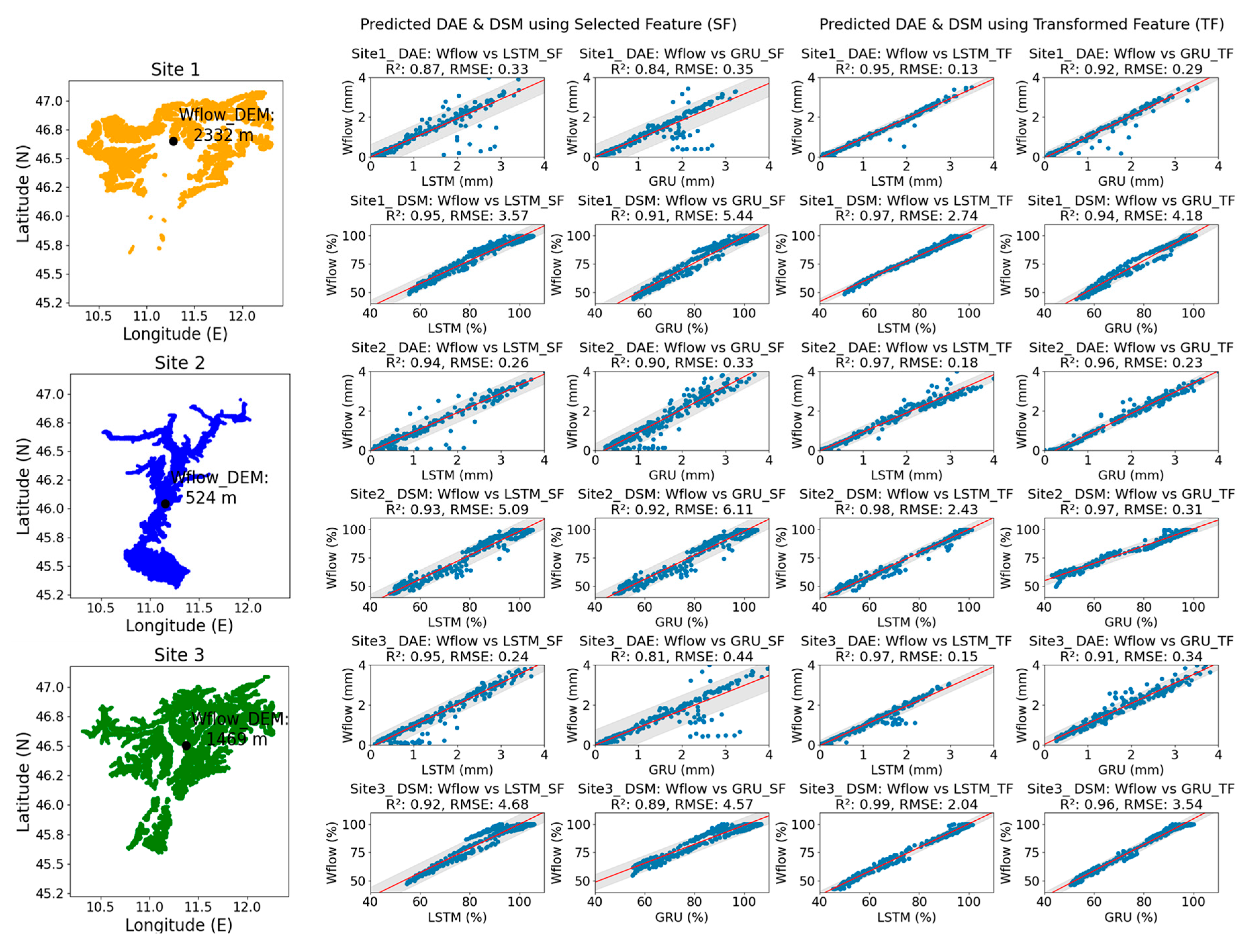
A comparison between LSTM and GRU models reveals that the calibrated parameters stabilize the predictions, making the results less sensitive to the model architecture. This finding indicates that even simpler models can achieve significant performance gains through the integration of adjusted parameters, highlighting the value of parameter transformation in improving model accuracy. For DSM predictions, the absolute residuals during training and testing with selected parameters reach maximum values between 12.5% and 15%. In contrast, applying transformed parameters reduces these biases to below 7.5%. To investigate the bias in estimating DAE and DSM using SDL models across temporal scales, results based on selected and transformed parameters were compared. The centroids of clusters derived from applying the FCM method to elevation data were chosen to represent distinct areas. This approach aimed to provide a clear visualization of results for a single representative pixel (site) that is more homogeneous with other points within its subregion.

Figure 17 presents regression plots that evaluate the degree of fit between the predicted data and the Wflow ground truth data. The analysis considered three representative sites at elevations of 2332 m, 524 m, and 1469 m. The results indicate a higher occurrence of outlier points obtained when predicting DAE using selected parameters compared to DSM. In this context, the LSTM model outperformed the GRU model. However, incorporating transformed parameters into both models led to more consistent predictions for DAE and DSM. This improvement is evident in the stronger regression fit relative to the Wflow ground truth data. Across all cases, the model accuracy exhibited R² scores ranging from 0.91 to 0.99, highlighting the effectiveness of parameter transformation in enhancing predictive performance.

7. Conclusions

This study tackles the challenge of calibrating surrogate deep learning (SDL) hydrological models across spatiotemporal scales to accurately predict high-quality data, such as daily actual evapotranspiration (DAE) and daily soil moisture (DSM). The modeling process begins by simulating hydrological outputs using climate parameters as dynamic inputs, with wflow-generated DSM and DAE data over the Adige catchment (Italy) serving as a representative case study for mountainous regions.

To enhance parameter calibration, a comprehensive computational pipeline is introduced, integrating techniques such as feature-level fusion of hydrological data, catchment regionalization via Fuzzy C-Means (FCM) clustering, and parameter transformation using Gradient Boosting Regression (GBR). To ensure spatial coverage of the proposed method, the GBR model was deployed in a distributed manner across homogeneous subregions defined by a Random Forest classifier. The subdivision of the catchment is guided by the static parameter Wflow_dem, which demonstrated a high importance of 60% in the calibration process. A further density analysis of Wflow_dem across subregions provided valuable insights into model reproducibility and parameter reliability. Significant improvements in the quality of the static parameter were observed when compared to the ground truth data. These improvements were particularly notable for parameters such as N, RootingDepth, and Swood in the case of DAE and for Slope, thetaS, and thetaR in the case of DSM.

Various unsupervised fusion models were also evaluated based on their ability to map hydrological data using statistical properties. The Adjusted Rand Index (ARI) was used to assess the alignment between clustering results derived from real and reduced-scale representations. High ARI scores were observed, with 0.71 for DAE using the t-SNE model and 0.78 for DSM using the Autoencoder model. To evaluate the effectiveness of the transformed approach across different SDL architectures, including LSTM, GRU, TCN, and ConvLSTM, the number of training epochs was fixed at 50. This ensured a consistent and fair comparison across models, allowing performance gains to be clearly measured. The results demonstrated improved accuracy and consistency compared to using parameters before transformation. This finding underscores the potential of the proposed approach for minimizing SDL model complexity while achieving high accuracy.

Further analysis with simpler models, such as LSTM and GRU, revealed notable improvements: DAE accuracy increased by 42%, while DSM accuracy improved by 36%. A temporal analysis of daily time series data was conducted by selecting centroid points from three distinct clusters based on Wflow_dem data. The results revealed the presence of the outlier’s residuals data when predicting DAE using the selected parameters. However, incorporating adjusted parameters significantly improved the model accuracy for both DAE and DSM, with R² scores ranging from 0.91 to 0.99. These findings highlight the effectiveness of parameter transformation in reducing prediction errors and enhancing the accuracy and reliability of hydrological models across different scales.

Future work could involve considering aridity to further refine calibrated parameters for improving the robustness of the model to large-scale prediction, particularly in regions characterized by diverse climatic zones.