Exploring Seasonal and Diurnal Variations of the Thermal Environment in Metropolitan Scale Analysis Based on Remote Sensing Data

Abstract

Urban morphology, including land surface, building heights, vegetation, water bodies, and terrain, exerts a significant influence on the urban thermal environment. The complex and nonlinear pathways through which these factors exert influence present significant challenges in urban climate studies. However, existing studies of statistical approaches to the urban thermal environment have primarily focused on linear relationships, often overlooking the complex and nonlinear effects of these factors. Additionally, previous research on those approaches has not adequately addressed the seasonal and diurnal variations in land surface temperature, nor has it examined the extent to which urban morphology influences these variations. While simulation-based approaches can address these nonlinearities and temporal variations, they require large parameter sets and extensive high-resolution input data, making them computationally demanding. This gap limits the ability to develop targeted and effective urban heat mitigation strategies. Recent advancements in remote sensing technologies have revolutionized our ability to analyze these complexities using medium-resolution data products. In this study, we apply a polynomial regression model with an elastic net to represent the impact of terrain and urban morphological factors on the urban thermal environment, considering its seasonal and diurnal variations, taking the case of the Osaka Metropolitan Area. This approach is unique in terms of capturing the nonlinearity of the impacts based on earth observation data by remote sensing and efficiently captures complex relationships while maintaining interpretability and reducing computational overhead. The study leverages MODIS Terra thermal infrared data from 2018, supplemented by Sentinel-2 and Copernicus Land Cover data. The results reveal significant seasonal and diurnal variations in the thermal environment, indicating that building height influences LST non-monotonically, with daytime cooling effects in dense urban areas (0.12 to 0.19 °C decrease) but nighttime heat retention in suburban zones (0.06 to 0.13 °C increase). Similarly, vegetation coverage reduces nighttime LST more effectively, particularly beyond a critical density threshold (NDVI > 0.4). These findings suggest that by optimizing urban design by considering building height effects, strategic design of vegetation coverage can help mitigate heat/cold stress and improve thermal comfort throughout seasons. These findings contribute to sustainable urban development and heat mitigation efforts by providing data-driven insights into urban morphology’s impact on the thermal environment.

1. Introduction

Urbanization has substantially intensified the urban heat island (UHI) effect, a phenomenon wherein urban areas exhibit elevated temperatures relative to their rural counterparts [1]. This effect is generally more pronounced in climates when the surroundings are covered by dense vegetation. This thermal anomaly results from the transformation of vegetated landscapes into impervious surfaces such as concrete and asphalt, which exhibit high thermal absorptivity and retain heat by absorbing solar energy during the day and releasing it gradually at night [2,3]. The implications of UHI are profound, encompassing increased energy consumption in summer, degraded air quality, heightened public health risks, increased pressure on water resources, the potential exacerbation of social inequalities, vulnerabilities within urban areas, and exacerbated climate change effects [4]. The intensity of UHI, as estimated from land surface temperature (LST), is usually referred to as the surface urban heat island (SUHI) [5].

High-rise structures exacerbate nocturnal heat retention through the “urban canyon effect”, which traps outgoing longwave radiation and impedes natural ventilation [6,7]. Conversely, building shadows are considered to have a substantial impact on thermal comfort and heating/cooling energy consumption [8]. Additionally, water bodies within urban areas contribute to thermal regulation through evaporative cooling during the daytime, yet their inherent thermal inertia can result in heat retention during nocturnal hours [9]. Vegetation serves as a critical mitigating agent, as it reduces LST through mechanisms such as shading and evapotranspiration [10]. Quantitative assessments employing metrics such as the Normalized Difference Vegetation Index (NDVI) consistently demonstrate robust inverse correlations between vegetation cover and LST [11,12]. Chakraborty and Lee [13] produced a multi-year monthly surface UHII dataset encompassing almost 10,000 cities worldwide. Building upon this data, they analyzed spatial and temporal patterns in surface UHI effects, exploring their relationship with vegetation indices.

In addition, topographical features also play a significant role in UHI dynamics, digital elevation models (DEMs) facilitate the analysis of topographic modifications to UHI patterns, with evidence indicating that higher altitudes exhibit reduced temperatures due to decreased air density, while topographical variation influences airflow, ventilation, and cold-air drainage, thereby regulating heat dispersion [14].

The advent and proliferation of remote sensing technologies have revolutionized UHI research by enabling detailed, multi-scalar analyses of urban thermal dynamics. Satellite platforms such as Moderate-Resolution Imaging Spectroradiometer (MODIS) have been instrumental in providing wide range/mid-resolution LST data, enabling comprehensive examinations of UHI intensity and variability across spatial and temporal domains [15]. The study by Yang et al. [16] highlights the importance of integrating multi-source datasets, comparing temperature data from platforms such as Terra and Aqua under different weather conditions. These comparisons reveal how data acquisition time, processing methodologies, and weather conditions influence UHI analyses, emphasizing the need for consistency in metropolitan-scale studies. This has proven particularly valuable in elucidating diurnal and seasonal variations in UHI phenomena, which are critical for understanding the underlying mechanisms and identifying effective mitigation strategies [15].

Several other remote sensing platforms also provide nighttime LST observations, each with unique advantages. For example, the ECOSTRESS (Ecosystem Spaceborne Thermal Radiometer Experiment on Space Station) offers high-resolution thermal data focusing on surface energy fluxes, making it particularly useful for studying fine-scale urban thermal dynamics [17]. Studies have leveraged ECOSTRESS data to assess urban heat vulnerabilities and inform mitigation strategies in cities like Los Angeles. Similarly, the Visible Infrared Imaging Radiometer Suite (VIIRS) provides improved spatial resolution compared to MODIS, making it valuable for analyzing nighttime LST patterns [18]. Research has demonstrated the potential of combining ECOSTRESS and VIIRS data to enhance land surface temperature mapping [19]. Other datasets, such as Landsat thermal infrared sensors, offer higher spatial resolution but have lower temporal frequency, limiting their usability for capturing diurnal variations. Nonetheless, Landsat data have been instrumental in characterizing urban land changes and their impact on surface temperatures. Despite the availability of these datasets, MODIS remains widely used in urban heat studies due to its continuous, long-term record and consistent spatial and temporal resolution. Given the study’s focus on analyzing both seasonal and diurnal variations in LST over an extended period, MODIS was selected as the primary dataset due to its suitability for long-term monitoring. However, recognizing the advantages of higher-resolution nighttime observations, future research could benefit from integrating MODIS with ECOSTRESS or VIIRS to refine spatial analysis and improve nighttime LST modeling.

Building on these technological advancements, global studies have shown that UHI dynamics vary significantly based on local conditions, such as urban density and land cover configurations. For instance, extreme SUHI intensities, surpassing seasonal averages by up to 16 kelvins, have been observed under specific urbanization and meteorological conditions [20]. These findings underscore the role of localized urban features, such as compact building structures, green spaces, and water bodies, in influencing SUHI magnitude. Notably, the dual role of water bodies demonstrates the necessity of diurnal and seasonal analyses to capture such nonlinear thermal behaviors. For instance, coastal cities show reduced SUHI intensities due to sea breeze effects, which can be inhibited by tall seafront buildings [21,22].

Despite advancements in UHI research, many studies have focused on isolated factors, such as vegetation or urban morphology, without sufficiently exploring their interactive effects on LST [23,24]. The interplay between vegetation, water bodies, topographical features, and urban morphology (e.g., building heights) remains underexplored in compact urban environments [25]. Some studies analyze the effects of multiple factors simultaneously [26], but they assume linear impacts of these factors on LST, which oversimplifies the complexity of urban thermal dynamics. Given the complexity of the mechanisms by which these factors influence LST, it may be necessary to explore more flexible modeling approaches that can potentially capture nonlinear or non-monotonic impacts. Recent evidence demonstrates the need to move beyond linear assumptions. Nonlinear relationships between SUHI intensity and environmental factors clearly illustrate that variables influencing LST and SUHI interact dynamically. Manoli et al. [27] developed a coarse-grained model to explain global patterns of urban-rural surface temperature differences (ΔTs). Their findings show that SUHI magnitude arises from the interplay of population density, climate conditions, and environmental background rather than being a straightforward function of any single factor. For example, in wet climates, evapotranspiration differences are constrained by energy availability, while in arid climates, water scarcity diminishes rural evapotranspiration, reducing ΔTs. These findings emphasize the necessity of exploring nonlinear interactions to fully understand SUHI dynamics and develop accurate predictive models. Simplistic assumptions of linearity risk overlooking critical thresholds and feedback mechanisms that govern urban heat patterns. For instance, average building height, a proxy for impervious surfaces and thermal storage, demonstrates contrasting effects by also providing shading, which mitigates solar radiation. By studying such nonlinearities, researchers can capture the nuanced and multi-faceted influences shaping urban thermal environments [28].

Numerical models of the urban heat environment have significantly advanced our understanding of UHI dynamics, particularly nocturnal thermal conditions [29]. These models offer high accuracy in predicting urban heat patterns but require extensive input data and substantial computational power, which limits their applicability across diverse cities and scenarios. Our approach leverages statistical techniques to identify the relationships between urban components and the thermal environment using remote sensing data, enabling us to estimate the impacts of urban space modifications [30,31]. While advancements in remote sensing platforms, such as MODIS and Sentinel, offer unprecedented opportunities for analysis, challenges related to data integration and resolution inconsistencies hinder their broader application. Chakraborty and Lee [13] leveraged the simplified urban-extent (SUE) algorithm to create a global database of SUHI intensity, capturing diurnal and seasonal patterns across climate zones over the entire MODIS mission (2003–2019). Their study found that daytime SUHI intensity has increased globally at a rate of 0.03 °C per decade, with significant variations linked to background climate conditions and their driving factors. Daytime SUHI was observed to be higher than nighttime SUHI in non-arid regions, with intensities peaking during the boreal summer where Eastern Asia shows the strongest rise, which can be linked to the rapid urbanization in the region [32]. These knowledge gaps are obstacles for comprehensive, regionally adapted strategies that integrate urban greening, cooling interventions, and energy-efficient urban planning to effectively mitigate UHI effects [3].

To address existing research gaps, this study explores the impact of urban morphological factors on LST, with a precise focus on diurnal and seasonal variations. The originality of this research lies in its data-oriented approach using flexible modeling techniques. Specifically, we employ moderate-resolution remote sensing data products from MODIS and Copernicus. Using this ensembled dataset, we apply polynomial regression analysis with elastic net regularization. This flexible modeling technique enables us to capture the diurnal (day and night) and seasonal (spring, summer, fall, and winter) variations in the mechanisms shaping thermal environments while accounting for the nonlinearity of impact factors.

This procedure is demonstrated for the case of the Osaka Metropolitan Area. As the employed data products are widely available for most cities around the world, the proposed method can be applied to other cities without significant challenges in data acquisition. Based on the estimated model, we discuss strategies for mitigating and managing the thermal environment across the Osaka Metropolitan Area.

The structure of this paper is as follows: Section 2 describes the study area, data employed, and method for polynomial regression and elastic net. Section 3 presents the results, including the estimated model performance, sensitivities of explanatory variables, and spatial distribution of estimation error. Section 4 discusses the implications of the model analysis for the thermal environment and potential mitigation policies. Finally, Section 5 concludes the study.

2. Materials and Methods

2.1. Study Area

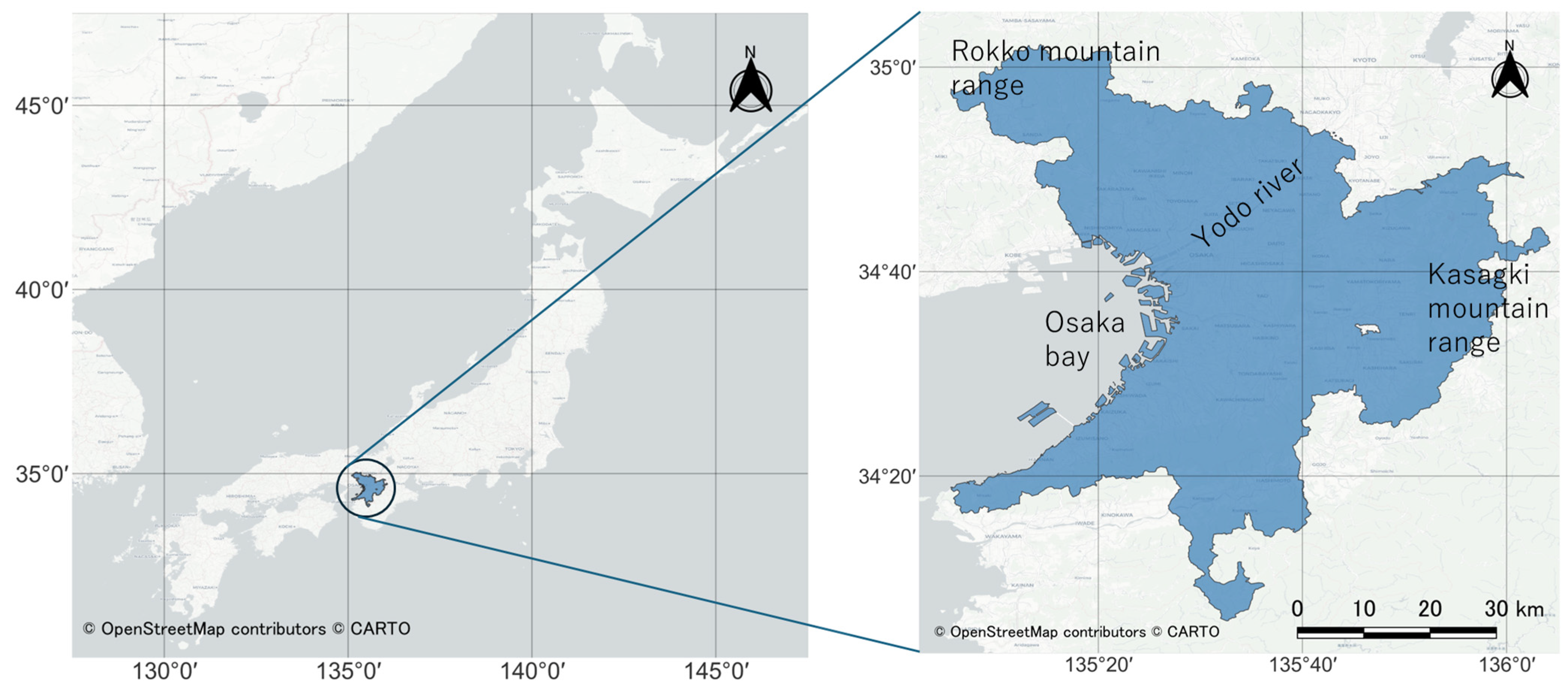
Osaka, a major economic hub in the Kansai region of Japan, is part of the second-largest urban agglomeration in the country. In this paper, we defined Osaka as the urban employment area (UEA) [33], which represents the commuting zone. The Osaka UEA consists of 12 million residents in a 3844 km² area (Figure 1). It is situated on a coastal plain by Osaka Bay and is bordered by the Rokko and Kasagi mountain ranges. This UEA consists of 75 municipalities including Osaka and Nara, and the region is characterized by extensive urbanization and intersected by major rivers like the Yodo. The area experiences a humid subtropical climate [34], with hot, humid summers, mild winters, and significant rainfall during the June-July rainy season [35]. Due to high-density urban development and climate change, the average temperature in the study area has shown an increasing trend over the past 30 years. For instance, the annual number of hours with temperatures exceeding 30 degrees celsius was 210 h in the 1980s but increased to 420 h in the period from 2006 to 2010 at the center of the Osaka Metropolitan Area. These attributes render Osaka an ideal case study for urban and environmental investigations.

2.2. Data

This study examines seasonal and diurnal variations, focusing on the year 2018 to ensure consistency and comparability across datasets.

Table 1. Variables and data sources.

Variables	Description	Resolution	Observed Period	Sources
LST	Land Surface Temperature/8-day composite data	1 km	1 January 2018 to 31 December 2018	MOD11A2 (NASA Earthdata: https://earthdata.nasa.gov, accessed on 1 November 2024)
NDVI	Normalized Difference Vegetation Index/bi-weekly data	250 m	1 January 2018 to 31 December 2018	MOD13Q1 (NASA Earthdata https://earthdata.nasa.gov, accessed on 1 November 2024)
DEM	Elevation data NASADEM_HGT topographic analysis, 1 arc second spacing	1 arc second	-	NASA DEM USGS Earth Explorer https://lpdaac.usgs.gov/products/nasadem_hgtv, accessed on 1 November 2024
Building height	Urban morphology data from Copernicus GHSL	100 m	2018	Copernicus GHSL (Global Human Settlement Layer https://ghsl.jrc.ec.europa.eu, accessed on 1 November 2024)
Water body	Spatial distribution of water bodies from Copernicus Land Cover	10 m	2018	Copernicus Land Cover (Global Land Cover Data—https://land.copernicus.eu/global/products/lc, accessed on 1 November 2024)
Major water body distance	Distance to the sea and other major water bodies calculated by author	100 m	2018	Copernicus Land Cover (Global Land Cover Data—https://land.copernicus.eu/global/products/lc, accessed on 1 November 2024)

outlines the key variables and datasets used in this analysis, providing details on their sources and characteristics. The MOD11A2 dataset provides 8-day composite LST data at a 1 km resolution under clear-sky conditions (with transit times at ~10:30 and ~22:30 local time), which reduces the noise present in single-day satellite observations and ensures more conservative estimations of temperature maxima and trends [36], enabling analysis of thermal patterns, including daytime and nighttime LST values. While UHI intensity can vary significantly between different parts of the same city, depending on their morphology and the thermodynamic properties of their elements (e.g., densely built-up areas versus green spaces) [37], spatial averaging helps mitigate the potential dilution of intensity felt locally. This approach also ensures a robust analysis of long-term thermal patterns while reducing the impact of short-term anomalies, such as extreme weather events or cloud cover interference.

The MOD13Q1 dataset offers bi-weekly vegetation indices at 250 m resolution, including the Normalized Difference Vegetation Index (NDVI), which provides accurate assessments in densely vegetated areas.

The Copernicus Global Human Settlement Layer (GHSL) dataset supplies 100 m resolution building height data, offering insights into urban morphology and its thermal impacts. We use the average gross building height (AGBH), which is calculated as the building volume divided by the grid area. This means that AGBH does not represent the average actual heights of individual buildings within the grid but rather the average height of the surface of the land. In other words, AGBH includes not only buildings but also other surfaces such as roads, parks, and open spaces [38]. The Copernicus Land Cover dataset, at 10 m resolution, categorizes water bodies, including inland and coastal features. Additionally, NASA’s DEM provides elevation data to assess topographic influences on thermal patterns.

Data for this study was obtained from NASA Earthdata and Copernicus platforms, ensuring high reliability and accuracy. Preprocessing steps, including reprojection, quality control, cloud masking, and aligning datasets, were carried out in R version 4.4.1, with R studio 2024.12.0, to guarantee consistency across all data layers. The study area is defined as the urban employment area (UEA) of Osaka, which represents a functional urban region characterized by commuting flows and economic activity. To ensure coherence and comparability, all datasets were aligned to a unified coordinate reference system during the analysis. Datasets included LST, NDVI, building height, DEM, and water body rasters, all processed using R packages such as sf, raster, terra, and dplyr. LST values were converted from Kelvin to celsius to enhance interpretability. Datasets were grouped into four seasons based on specific Day of Year (DOY) ranges, Dividing the year into four periods: spring spans DOY 60–151 (March–May), summer spans DOY 152–243 (June–August), fall spans DOY 244–334 (September–November), and winter spans DOY 335–59 (December–February) with diurnal adjustments made for local solar time to account for satellite overpass timings. Static datasets, such as DEM, building height, and water body data, were processed independently of temporal classifications. All raster layers were aligned to the 3.57 arc second resolution of the GHSL data using bilinear interpolation under latitude-longitude projection with WGS84 datum, while nearest-neighbor interpolation was used for categorical data, after preprocessing, the number of pixels (grids) varied slightly across datasets due to differences in data availability and coverage. The LST dataset contained 379,700 grids, while NDVI ranged from 379,560 to 379,693 grids across seasons. The DEM and water body layers included 378,180 grids, while the building height dataset consisted of 3 83,779 grids. The distance to major water bodies was calculated for 383,873 grids. Rather than using the full extent of the original imagery, the study area was limited to the Osaka Metropolitan Area, ensuring consistency. LST, Seasonal NDVI, DEM, and water body rasters were resampled, and a distance index for major water bodies (sea proximity) was computed to quantify their impact on urban heat dynamics. The datasets were stacked into a multi-layer framework for unified analysis.

Table 2. Descriptive statistics in the study area.

Variables	Season	Time	Grids	Mean	Median	Standard Deviation	Maximum	Minimum
LST (degrees celsius)	Spring	Day	379,700	22.75	22.49	4.15	31.602	14.27
		Night	379,700	10.24	10.17	1.10	13.69	6.52
	Summer	Day	379,700	32.08	31.84	4.48	41.34	22.98
		Night	379,700	22.29	22.12	1.80	26.52	17.06
	Fall	Day	379,700	21.73	21.52	3.19	27.81	14.69
		Night	379,700	11.59	11.44	1.07	16.08	7.67
	Winter	Day	379,700	8.58	8.65	2.40	13.491	2.49
		Night	379,700	1.19	1.12	0.82	4.60	−1.40
NDVI (ratio 0–1)	Spring		379,693	0.44	0.46	0.18	0.85	−0.16
	Summer		379,598	0.56	0.63	0.20	0.91	−0.09
	Fall		379,560	0.55	0.60	0.19	0.90	−0.16
	Winter		379,661	0.50	0.54	0.17	0.84	−0.12
DEM (meter)			378,180	184.92	119.92	185.40	1134	−13.46
Building height (meter)			383,779	2.10	0.16	3.04	52.44	0
Water body (%)			378,180	1.16	0	8.52	100	0
Major water body distance (meter)			383,873	7191.49	5985.14	3822.77	33386.07	0

shows the descriptive statistics of all variables for the study area. Statistical metrics provided in the table include the mean, representing the average value across all grid cells; the median, identifying the central value in the dataset; the standard deviation, which highlights data variability; and the maximum and minimum values, indicating the range of observed data.

The descriptive statistics reveal notable seasonal and temporal variations in LST. For instance, daytime LST peaks in summer with a mean of 32.08 °C, while the lowest nighttime temperature occurs in winter, averaging 1.19 °C. These findings highlight how seasonal variations directly shape the thermal dynamics in the region. NDVI values show the highest mean in summer (0.56), reflecting active vegetation growth, and the lowest mean in spring (0.44), indicative of less vegetation coverage during this period.

Topographical diversity is evident from the DEM statistics, with elevation values ranging from −13.46 m to 1134 m and a mean elevation of 184.92 m. This variation captures the complex terrain of the study area. Building heights demonstrate a predominantly low urban profile, with an average height of 2.10 m and a median of 0.16 m, suggesting that most areas are sparsely built up. Water body data indicate significant variability, with a mean value of 1.16 and a maximum value of 100. The proximity to major water bodies averages 7191.49 m but can extend as far as 33,386.07 m in some locations, highlighting hydrological patterns in the region.

These descriptive statistics form the basis for understanding the relationships between environmental and urban factors and their impact on LST. The dataset’s comprehensiveness enables robust estimation of the polynomial model, as outlined in Section 2.3, to analyze these interconnections effectively.

2.3. Methodology

Raster values were extracted from the aligned dataset and converted into a data frame, preserving non-missing values for integration across LST, vegetation, morphological, and hydrological variables. The data were split into training (50%) and testing (50%) subsets to ensure robust model development and validation. The training data were used to establish relationships between LST and explanatory variables, while the test data validated predictive accuracy.

We employ a polynomial regression model to represent the nonlinearity and complexity of the impacts of factors on the LST. The higher-order polynomial increases its flexibility in fitting to the data. At the same time, it will cause overfitting. To find the balance between the flexibility and overfitting, we use elastic net [39] as a regularization tool and the Akaike Information Criterion (AIC) for model selection. The model is estimated for each seasonal and diurnal segment, i.e., eight models are estimated. Using the estimated models, we analyze the nonlinearity and sensitivity of each factor on the LST and seasonal/diurnal features of the urban thermal environment. 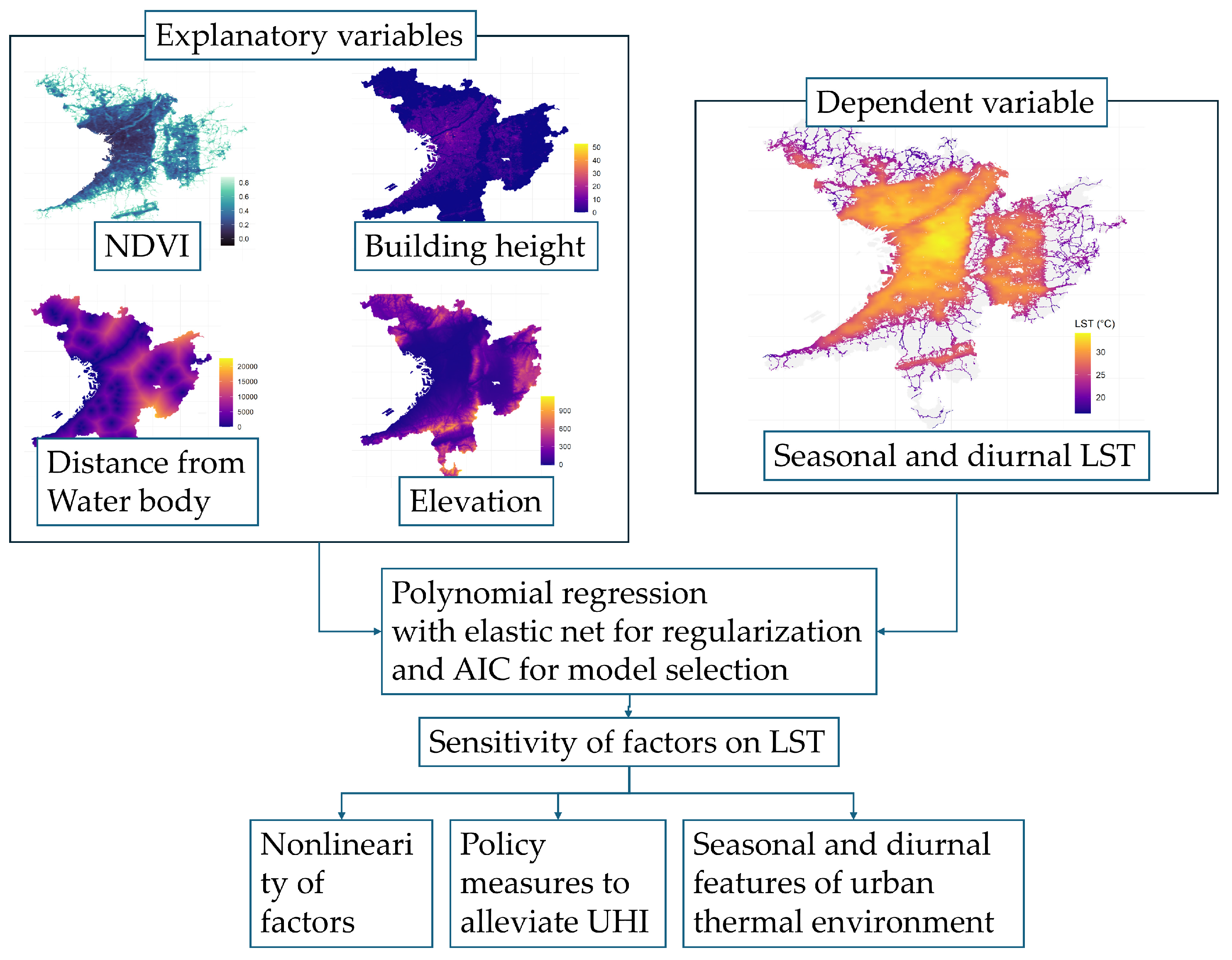Figure 2 shows the conceptual framework of the analysis in this study.

Polynomial terms of degrees from 1 to 10 are examined. First, the polynomial function is defined as follows:

$$f\left({\mathbf{x}}_i,\mathbf{\beta },Q\right)=\sum _{\left\{k_j|1\le j\le m\right\}\in {\rm K}}{\beta }_{k_1{k}_2\dots k_m}{x}_{i1}^{k_1}{x}_{i2}^{k_2}\dots x_{im}^{k_m}$$

(1)

$$\sum _{\mathit{j}}{k}_j\le Q$$

(2)

where ${\mathbf{x}}_i$ is the vector of explanatory variables at grid i, and $Q$ is the maximum order of the polynomial. ${\rm K}$ is a set of vectors of all combinations of order of each variable that satisfies Equation (2). $\mathbf{\beta }=\left\{{\beta }_{k_1{k}_2\dots k_m}\right\}$ is the vector of coefficients. Here, ${0\le k}_j\le Q$. In case $k_j=0 for \forall j$, ${\beta }_{k_1{k}_2\dots k_m}$ represents intercept. The coefficient estimation using the elastic net is given by the following equation:

$$\widehat{\mathbf{\beta }}=\arg \underset{\mathbf{\beta }}{\mathrm{m}\mathrm{i}\mathrm{n}}\left({\sum }_{i\in \Omega }\left\{{\left(y_i-f\left({\mathbf{x}}_i,\mathbf{\beta },Q\right)\right)}^2\right\}+\lambda \left(\alpha ‖\mathbf{\beta }‖+\left(1-\alpha \right)‖{\mathbf{\beta }}^2‖\right)\right)$$

(3)

Cross-validation optimized model parameters, including the mixing ratio ($\alpha$) and regularization strength (λ), which minimize the root mean square error (RMSE) for test data. $\Omega$ is a set of target grids. Here, the elastic net is a generalized class of regularization of parameter estimation, including LASSO regression ($\alpha =1$) and Ridge regression ($\alpha =0$).

We calculated the parameters for all maximum degrees $Q$ from 1 to 10 and chose the degree that minimize the Akaike Information Criterion (AIC). AIC is given by the following equation:

$$AIC=-2LL+2k$$

(4)

$$LL=-{\displaystyle \frac{1}{2}}\ln 2\pi {\sigma }^2-\left|\Omega \right|$$

(5)

where $LL$ is the log-likelihood of the model $f\left(\mathbf{x},\mathbf{\beta },Q\right)$, ${\sigma }^2$ is the variance of the model estimation error, $\left|\Omega \right|$ is the size of samples, and $k$ is the degree of freedom of the model. In this case, $k$ is the number of non-zero coefficients minus 1.

Sensitivity analysis systematically evaluates the influence of individual variables by varying their values within the reliable range of explanatory variables, isolating their effects on LST. We assume the reliable range of explanatory variables is their lower 95%. We apply average values for all explanatory variables other than the target variable to examine the sensitivity. The sensitivity plots highlighted the relative contributions of each factor.

Scenario analysis was conducted to assess the impact of urban morphological modifications on LST variations. Two scenarios were designed: increased building height, simulating the effect of higher structures while maintaining existing vegetation; and enhanced vegetation, modeling an increase in NDVI values to evaluate the cooling potential of urban greening. The trained regression model was used to predict LST variations under these scenarios, and the results were spatially analyzed in Section 3.3. This approach complements sensitivity by providing insights into potential urban planning strategies for mitigating heat stress.

Residual analysis examined prediction errors to identify potential model biases and unexplained spatial patterns. Residual maps and statistical plots were generated to assess model reliability and identify areas for improvement.

3. Results

3.1. Model Estimation

The results, presented in

Table 3. Performance metrics of elastic net regression models by season and time of day.

Season/Time	(λ)	(α)	Minimum AIC	Degrees Minimize AIC	Degree of Freedom	RMSE	R2
Spring (Day)	7.49 × 10−4	0.51	−2.95 × 106	8	438	1.19	0.91
Spring (Night)	7.33 × 10−5	1.00	−1.45 × 105	6	473	0.64	0.65
Summer (Day)	1.17 × 10−3	0.34	−3.42 × 106	10	423	1.33	0.90
Summer (Night)	2.12 × 10−4	0.72	−5.2 × 105	6	473	0.62	0.87
Fall (Day)	4.04 × 10−4	0.72	−1.75 × 106	7	455	0.83	0.93
Fall (Night)	5.27 × 10−5	1.0	−1.17 × 105	7	455	0.71	0.55
Winter (Day)	3.89 × 10−4	0.72	−8.89 × 105	10	423	0.91	0.85
Winter (Night)	6.56 × 10−5	1.00	−6.51 × 104	8	438	0.55	0.51

, highlight key statistical metrics, including the regularization parameters (λ and α), the Akaike Information Criterion (AIC), the polynomial degree minimizing the AIC, the degrees of freedom, the root mean square error (RMSE), and the coefficient of determination (R²). These parameters provide insights into model complexity, accuracy, and explanatory power for LST prediction in each scenario.

The regularization parameter λ, which controls the trade-off between bias and variance in the models, varied across seasons and times of day. Lower λ values, as seen in winter (night) (6.56 × 10⁻⁵) and spring (night) (7.33 × 10⁻⁵), indicate less penalization of model coefficients, allowing greater flexibility to capture complex relationships. In contrast, higher λ values, such as summer (day) (1.17 × 10⁻³), reflect stronger penalization, suitable for simpler predictor relationships. The elastic net mixing parameter (α), balancing the lasso (α = 1) and ridge (α = 0) components, showed variability across scenarios. It was predominantly set at either 1.0 or 0.72, with exceptions like 0.34 (summer day) and 0.51 (winter day), emphasizing that a flexible penalization scheme is needed to capture the complexity of LST formation by season and time.

The degree of the polynomial minimizing the AIC was determined separately for each season and diurnal period using the same dataset. This ranged from 6 to 10, reflecting varying levels of complexity required for optimal performance. The degrees of freedom in this analysis, defined as the number of non-zero coefficients in the model, ranged from 423 to 473. In the context of elastic net regularization, as implemented in the (cva.glmnet) function, degrees of freedom represent the number of effective parameters retained after regularization. This differs from the traditional definition of degrees of freedom (n − p) and instead reflects the balance between data flexibility and the constraints imposed by the penalty terms (α and λ).

Higher degrees of freedom, observed in models such as summer (day) and winter (day), suggest that more parameters were required to represent the data, likely due to intricate interactions among predictors in these conditions. Conversely, models with fewer degrees of freedom, such as spring (night) and summer (night), indicate simpler relationships between LST and the selected predictors. This interpretation highlights that in regularized models like elastic net, degrees of freedom are influenced by both the dataset and the regularization process rather than solely representing model flexibility in the conventional sense.

Model accuracy, as indicated by RMSE values, ranged from 0.55 to 1.33. Winter (night) demonstrated the lowest RMSE (0.55), highlighting strong predictive accuracy, while summer (day) exhibited the highest RMSE (1.33), reflecting greater variability by grids and complexity in daytime LST. These results suggest that seasonal and diurnal differences in LST predictability are influenced by factors such as meteorological conditions, land surface properties, and anthropogenic heat emissions.

The coefficient of determination (R²), measuring the proportion of variance explained by the model, highlighted notable differences in performance. Fall (day) had the highest R² (0.93), indicating strong predictive power, followed by spring (day) (0.91). Conversely, winter (night) had the lowest R² (0.51), reflecting weaker explanatory power, likely due to greater nocturnal variability, even though the RMSE is the lowest. Across all scenarios, daytime predictions consistently achieved higher R² values than nighttime predictions, underscoring the stronger influence of the chosen predictors, such as vegetation indices and urban characteristics, during the day. Oppositely, the other variables are required to explain the spatial distribution of the nighttime LST.

3.2. Sensitivity Analysis

3.2.1. LST vs. Building Height

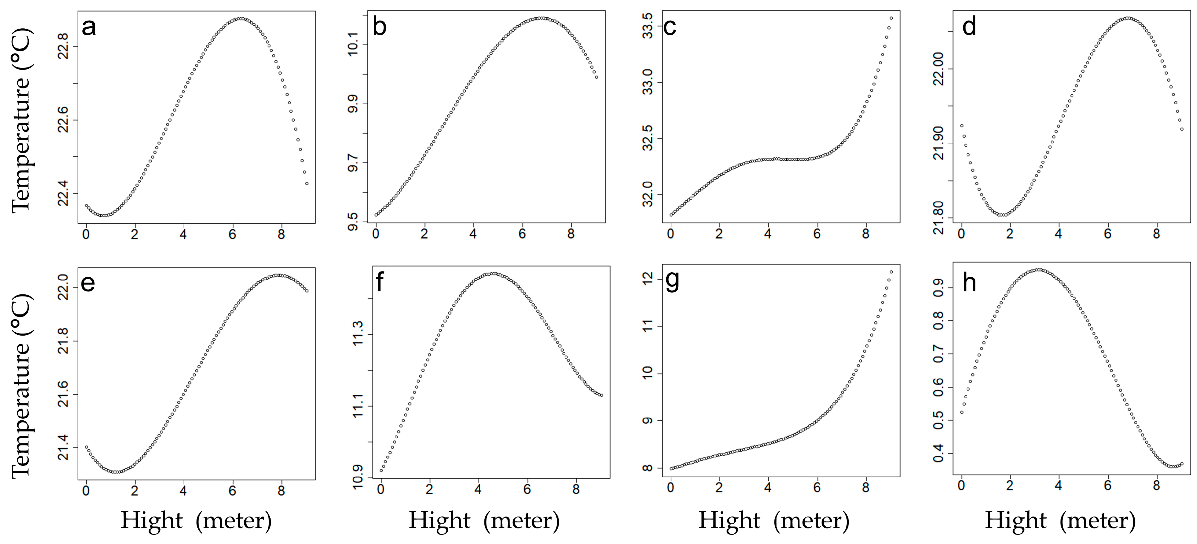
The sensitivity analysis, of which method is explained in Section 2.3, of building heights on average temperature, as shown in Figure 3, highlights the seasonal and diurnal variability of this relationship, as well as the differences in temperature ranges (LST variation) across scenarios.

In spring and fall daytime (Figure 3a,e), LST increases nonlinearly with height, peaking at approximately 6 m before slightly stabilizing or declining. The moderate temperature variations (22.4–22.8 °C in spring; 21.4–22.0 °C in fall) indicate a measurable but limited effect of building heights on LST during these periods. This trend reflects the combined influence of heat retention anthropogenic heat intensity at moderate heights and the redistribution of heat by shadows cast by taller buildings. Shadows likely block direct solar radiation at higher elevations, reducing surface heating and contributing to the slight decline in LST beyond the peak. At night (Figure 3b,f), the LST response is subdued, with smaller temperature variations (9.5–10.1 °C in spring; 10.9–11.3 °C in fall). Radiative cooling and minimal solar input likely drive this limited sensitivity during nighttime, with little additional influence from building heights.

Summer daytime (Figure 3c) displays a distinctive pattern, with LST increasing consistently with height initially, followed by a steady phase between 4 and 6 m, and then increasing again at greater heights. The temperature range (32.0–33.5 °C) highlights the pronounced impact of solar radiation and urban geometry. The steady phase at mid-heights may result from a balance between heat retention at building surfaces and reduced heat exchange processes, while the subsequent increase at higher elevations reflects intensified heat-trapping and increased solar exposure. The high solar angle in summer minimizes shadow effects, allowing direct solar radiation to dominate temperature dynamics. Summer nighttime (Figure 3d) exhibits a delayed cooling trend, with temperatures peaking at mid-heights (21.8–22.0 °C). This reflects cumulative heat storage during the day and reduced radiative cooling due to urban heat retention.

Winter daytime (Figure 3g) exhibits the highest temperature variation across all seasons, with changes up to 4 °C. This consistent increase in LST with building height is attributed to the larger exposed building surfaces absorbing and retaining heat during the day. Despite weaker solar intensity in winter, urban materials store heat efficiently, resulting in a pronounced temperature gradient with building height. Additionally, reduced heat dissipation mechanisms, such as limited cooling effects, may amplify the effect of building heights on LST. Winter nighttime (Figure 3h) shows minimal sensitivity to building heights, with LST variations ranging from 0.4 °C to 0.9 °C. Radiative cooling dominates during this period, and the absence of significant heat input results in nearly uniform temperature distributions with height.

3.2.2. LST vs. NDVI

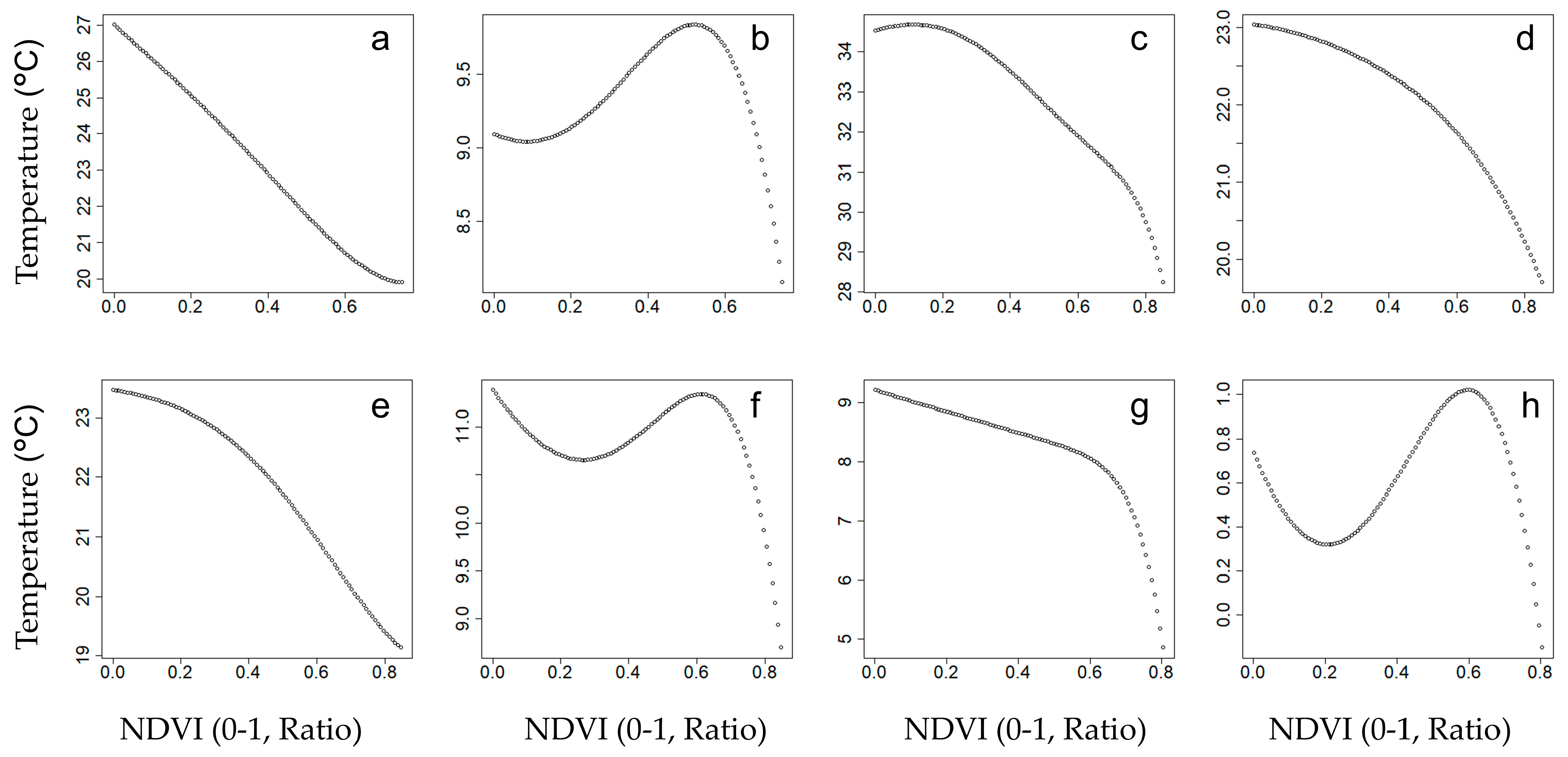
The sensitivity analysis of NDVI versus LST is shown in Figure 4. The interaction between vegetation and LST highlights differences in temperature ranges (LST variation) across scenarios.

In spring and fall daytime (Figure 4a,e), LST demonstrates a consistent decrease with increasing NDVI, ranging from 27 °C to 20 °C in spring and 23 °C to 19 °C in fall. This trend reflects the cooling effects of vegetation through shading and evapotranspiration, which mitigate urban heat during these periods. The patterns in both seasons are nearly identical, reflecting their transitional characteristics and moderate solar radiation. At night (Figure 4b,f), the response is less pronounced, with LST ranging from 9.5 °C to 10.5 °C in spring and 11 °C to 10 °C in fall. These smaller variations indicate reduced vegetation influence at night due to minimal evapotranspiration and weaker temperature gradients.

Summer daytime (Figure 4c) exhibits the steepest decline in LST with increasing NDVI, ranging from 34 °C to 28 °C. However, this relationship is nonlinear, as LST remains nearly constant within the NDVI range of 0 to 0.2, suggesting that sparse vegetation in densely built-up areas provides limited cooling. Beyond this threshold, vegetation significantly mitigates extreme heat through shading and evapotranspiration. At night (Figure 4d), the cooling effect is weaker, with LST ranging from 23 °C to 20 °C, reflecting the persistence of heat in less vegetated areas and the ability of vegetation to enhance nocturnal cooling.

Winter daytime (Figure 4g) also shows a significant negative relationship, with LST decreasing from 9 °C to 5 °C as NDVI increases. The cooling effect is evident, though less pronounced, due to reduced solar input. At night (Figure 4h), the sensitivity is minimal, with LST ranging from 1 °C to −2 °C, as vegetation has a limited influence in the absence of heat input and evapotranspiration during colder months.

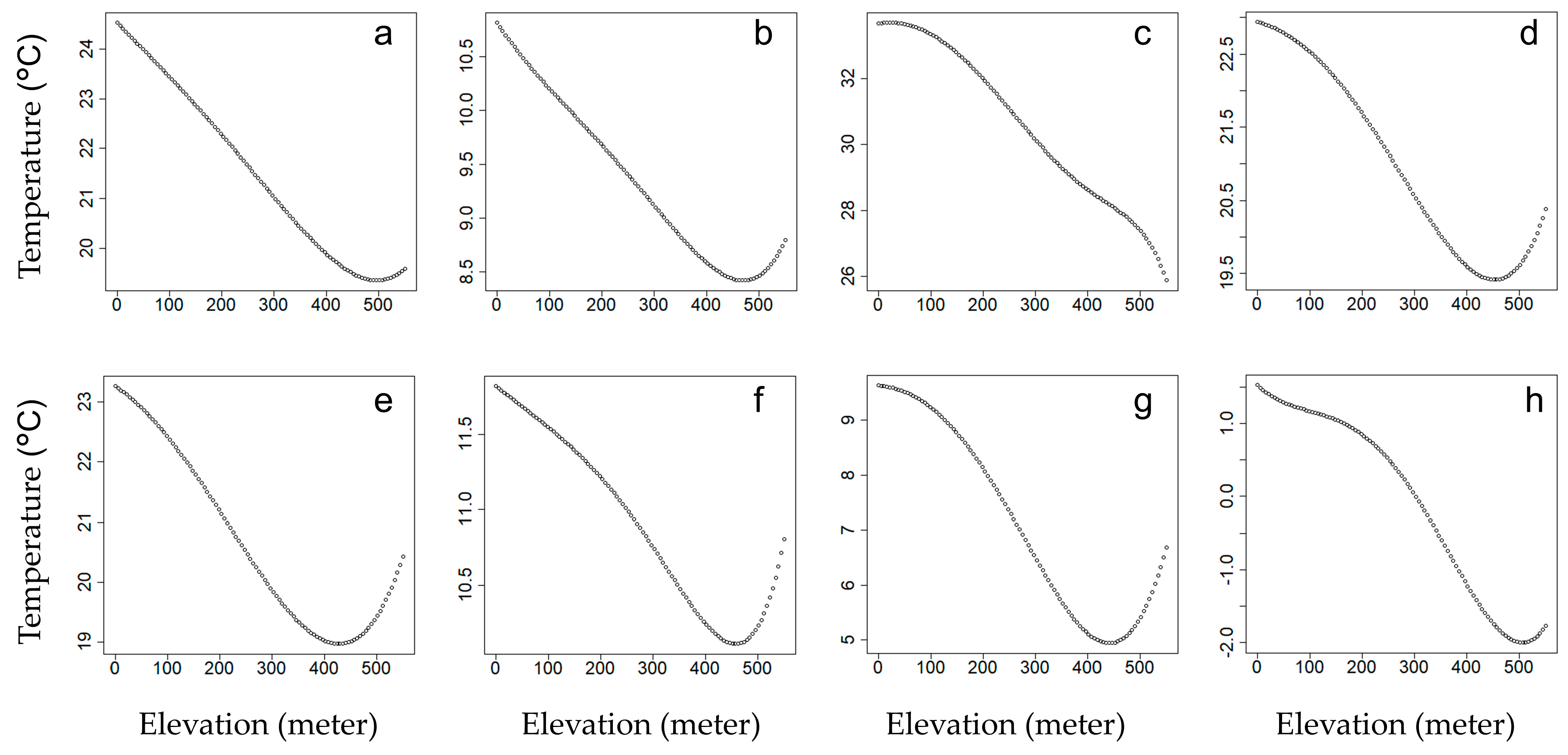
3.2.3. LST vs. DEM

The analysis of DEM versus LST, as shown in Figure 5, highlights how elevation consistently influences LST across seasons and times of day.

The graphs indicate a clear negative relationship between DEM and LST, where higher elevations correspond to lower temperatures. This trend reflects the typical lapse rate, where temperature decreases with altitude due to reduced atmospheric pressure and density. The steepness of this decline varies slightly between daytime and nighttime, with daytime generally exhibiting stronger temperature decreases compared to nighttime. This pattern is more pronounced during summer, where higher elevations mitigate extreme heat effectively, with temperatures ranging from approximately 34 °C at lower elevations to 26 °C at higher elevations. In winter, the overall temperature range is smaller due to weaker solar input, but the cooling effect of elevation remains consistent, with daytime temperatures ranging from 9 °C at lower elevations to 5 °C at higher elevations.

Nighttime patterns show less sensitivity to elevation, with smaller temperature ranges observed across all seasons. This reduced sensitivity is attributed to limited solar heating and the dominance of radiative cooling during the night. For example, winter nighttime temperatures range from 1 °C at lower elevations to −2 °C at higher elevations, reflecting minimal variation compared to daytime trends.

Across all seasons, the role of elevation in mitigating heat is evident, particularly during daytime. Spring and fall display intermediate patterns, reflecting their transitional characteristics and moderate elevation influence. Summer shows the steepest decline in LST with increasing elevation due to intense solar radiation. Winter demonstrates a nonlinear trend similar to other seasons, with a consistent cooling effect, though not as steep as summer daytime.

Considering elevation’s consistent influence on LST, urban planning strategies should leverage the cooling benefits of higher altitudes, particularly in mitigating summer heat.

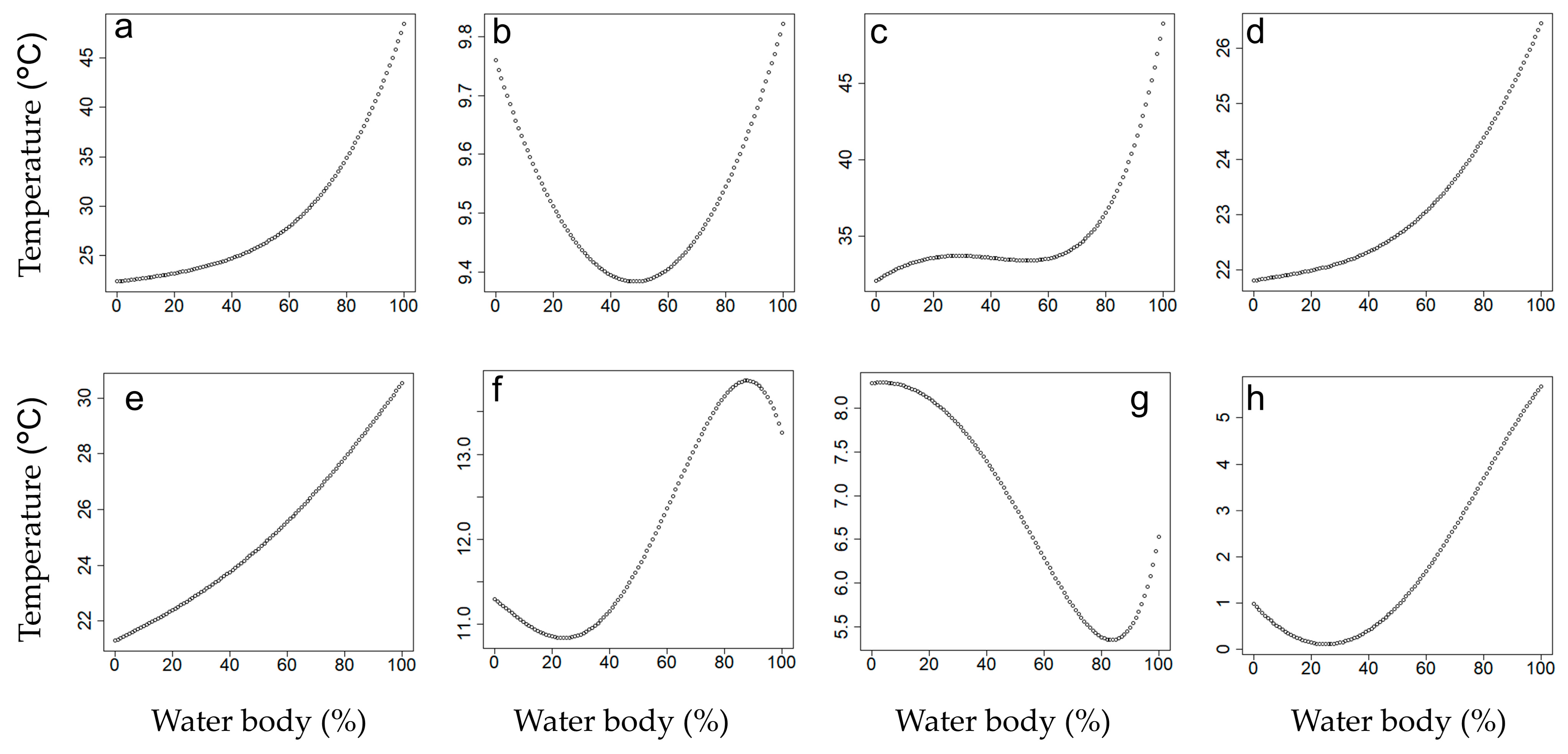
3.2.4. LST vs. Water Body

The analysis of water body percentage versus LST, as shown in Figure 6, highlights how the presence of water bodies influences LST across seasons and times of day.

The graphs reveal a mix of linear and nonlinear relationships between water body percentage and LST, depending on the season and time of day. During daytime in all seasons, a consistent positive correlation is observed, where higher water body percentages correspond to higher temperatures. This is particularly evident in summer daytime (Figure 6c), where LST increases steeply from 35 °C to 45 °C as the water body percentage rises, reflecting the heat-retaining properties of water and its ability to amplify surrounding temperatures under intense solar radiation. A similar pattern is observed in spring (Figure 6a) and fall daytime (Figure 6e), albeit with lower temperature ranges, indicating moderate heat amplification in these seasons. However, these figures represent only the results of a sensitivity analysis in which we assume that all other variables are fixed at their average levels across the study area. Of course, in reality, a higher waterbody percentage is likely associated with lower building heights and NDVI. In this analysis, however, those variables are held constant at their average values.

In contrast, nighttime graphs (Figure 6b,d,f,h) exhibit nonlinear trends, with LST initially decreasing with rising water body percentage, reaching a minimum, and then increasing again. This U-shaped relationship likely reflects the dual role of water bodies in dissipating heat through evaporation while also retaining and re-emitting heat during the night. For instance, in spring nighttime (Figure 6b), temperatures drop to a minimum of 9.4 °C before increasing as water body percentage exceeds 60%. Similarly, winter nighttime (Figure 6h) shows temperatures decreasing to a minimum of 0 °C at mid-range water body percentages, then rising to 4 °C as the percentage increases further.

Seasonal variations are also evident. Summer exhibits the strongest daytime heat amplification due to high solar intensity and the heat-absorbing properties of water, while spring and fall show moderate effects. Winter, with its lower solar input, demonstrates the least daytime sensitivity but maintains a notable nonlinear nighttime trend, suggesting that even under reduced heat input, water bodies influence nocturnal cooling and warming patterns.

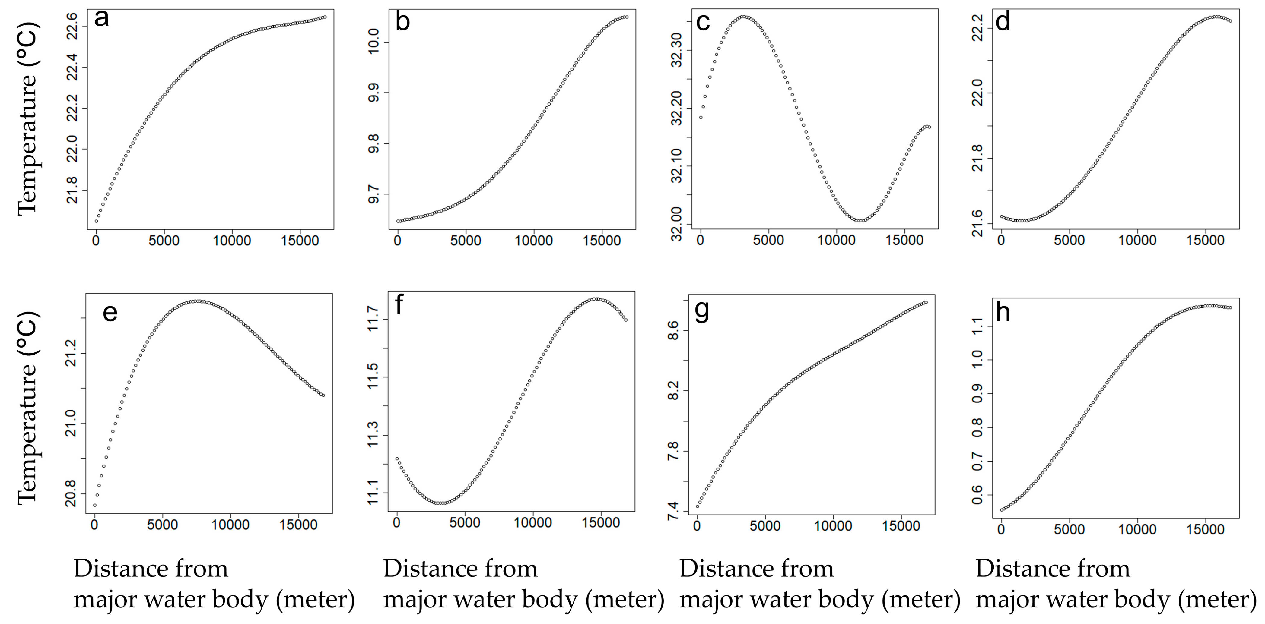
3.2.5. LST vs. Major Water Body Distance

Building on the understanding of water body percentage, the analysis of major water body distance versus LST in Figure 7 reveals how proximity to large water bodies further shapes LST patterns across seasons and times of day.

The graphs generally reveal a positive correlation between major water body distance and LST, where temperatures increase as the distance from a water body grows. This trend reflects the localized cooling influence of large water bodies, which moderate surrounding temperatures through evaporation and heat absorption. However, the magnitude of this effect is limited in most cases and varies by season and time of day.

During daytime, proximity to major water bodies correlates with lower LST, but the impact is minimal in some seasons. For instance, in summer daytime (Figure 7c), the relationship appears nonlinear, but the LST variation is small (~0.3 °C), indicating no significant effect. Similarly, spring (Figure 7a) and fall daytime (Figure 7e) show gradual increases in LST with distance from water bodies, with slightly larger but still moderate variations. By contrast, winter daytime (Figure 7g) demonstrates the strongest sensitivity, with LST varying by more than 1 °C, indicating that the cooling effects of water bodies are more pronounced in winter and diminish significantly at greater distances.

Nighttime graphs (Figure 7b,d,f,h) exhibit more complex and nonlinear trends. For example, in winter nighttime (Figure 7h), temperatures steadily increase from 0.6 °C to over 1 °C as the distance from water bodies grows, reflecting the reduced cooling effects of water bodies at greater distances. In fall nighttime (Figure 7f), LST decreases slightly near water bodies but increases at greater distances, reflecting the dual role of water bodies in nighttime cooling and localized heat retention due to re-radiation of stored heat. Across all seasons, nighttime effects are generally weaker compared to daytime.

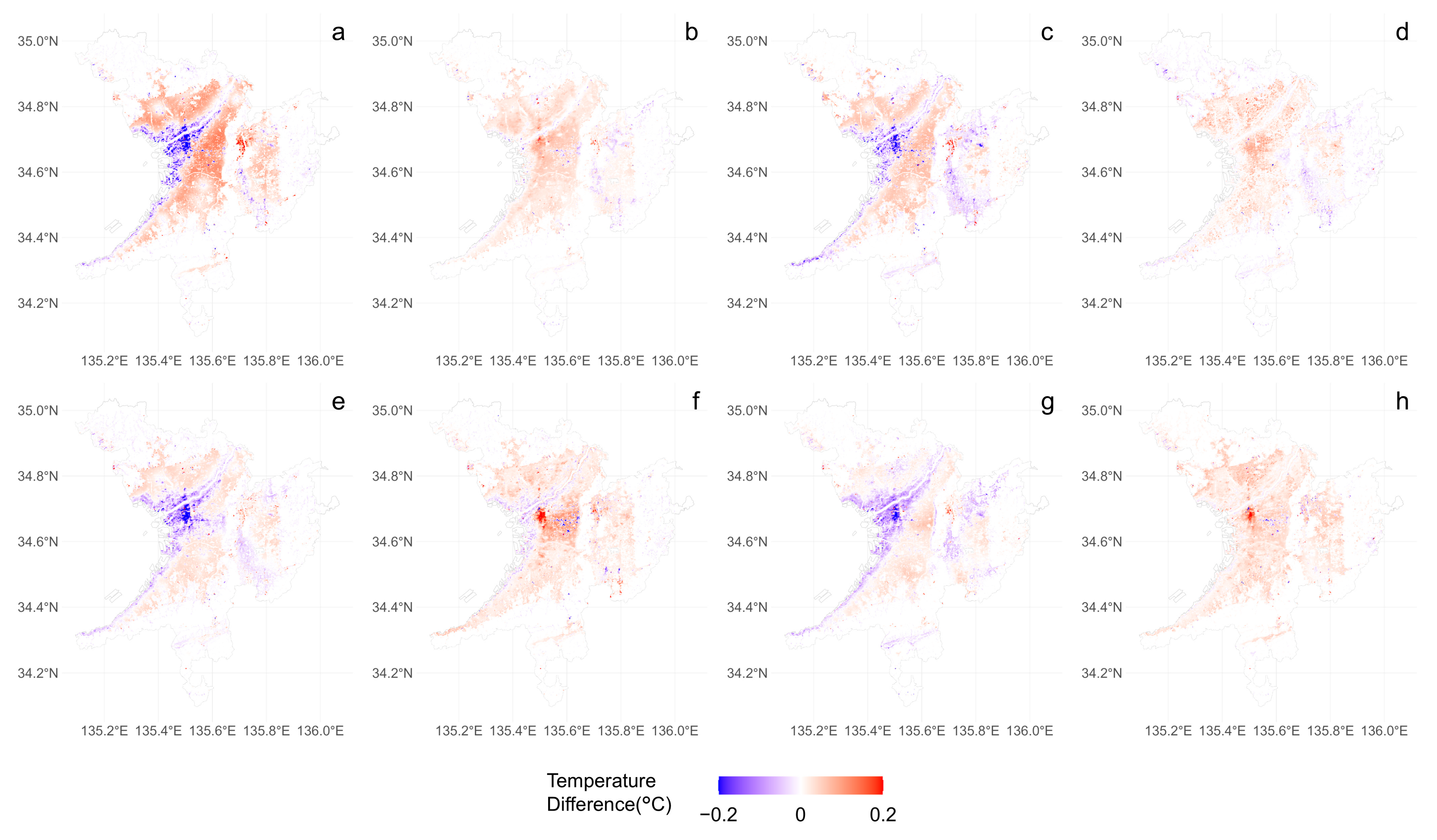
3.3. Scenario Analysis

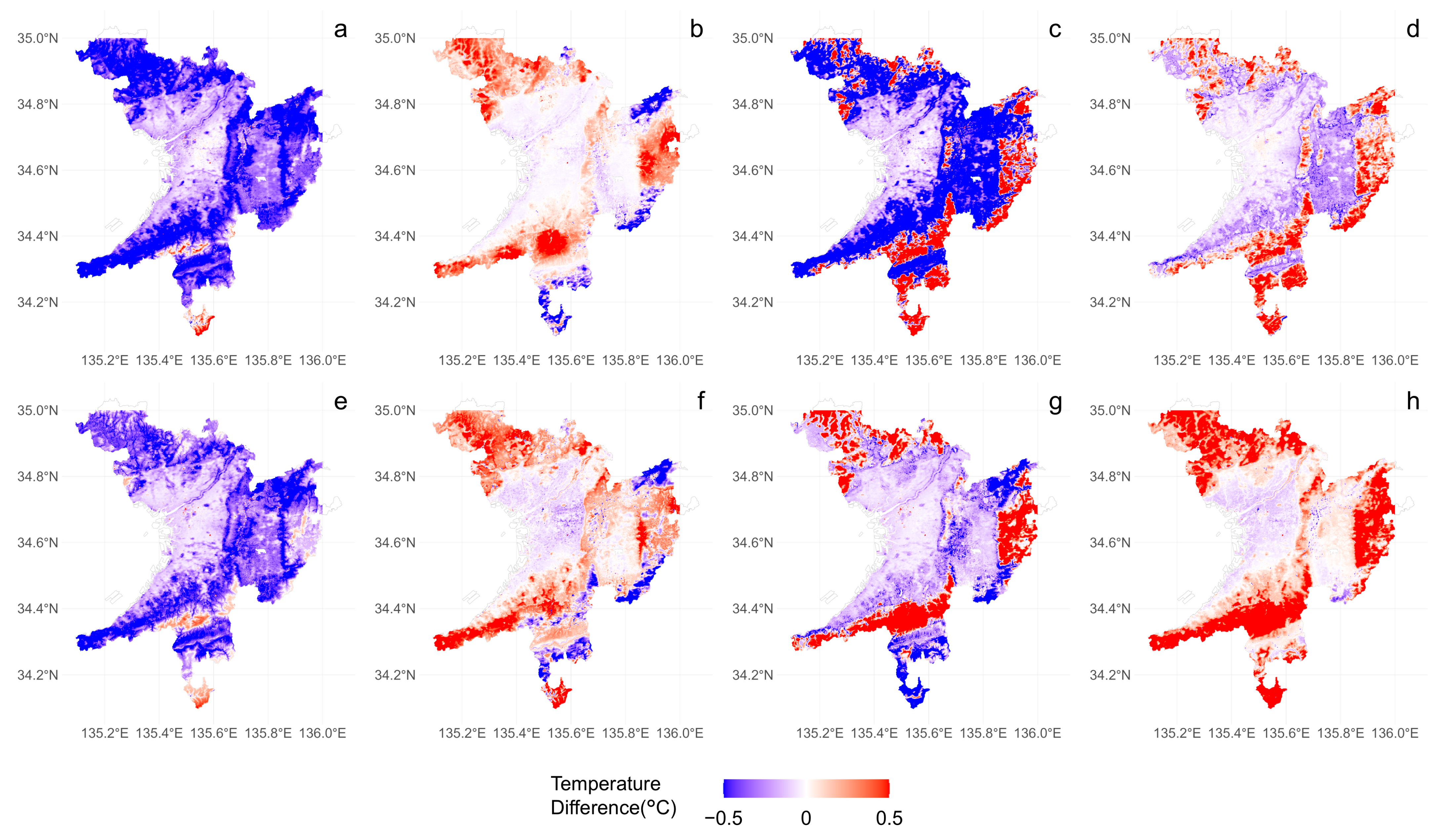
This section analyzes the scenarios of building height and NDVI; we estimate the spatial impacts of those values of each grid by 10% compared to the observed values.

Figure 8 indicates the changes in LST when building heights are increased by 10%. During the daytime (Figure 8a,c,e,g) across all seasons, the central urban areas are estimated to experience temperature reductions, while the suburban areas are estimated to increase the temperature. In contrast, during the nighttime (Figure 8b,d,f,h), temperatures are estimated to increase across most urban areas.

In the daytime cases, the results differ from the sensitivity analysis presented in Section 3.2.1, showing temperature reductions, particularly in the highly built-up central urban areas. This may be attributed to the higher-order polynomial approximations, which reveal trends differing from the average sensitivity due to interactions with other factors. In areas with significant high-rise development, the shading effects of tall buildings and the spatial composition of public open spaces organized through urban planning may influence the sensitivity of LST. Conversely, in suburban low-rise areas, where the proportion of public land including road space is lower than in the city center, a 10% increase in building height could lead to higher spatial building density and, consequently, an increase in LST.

At night, temperatures are estimated to rise across most urban areas regardless of the season. Since solar radiation does not influence nighttime conditions, factors such as increased heat retention due to greater building volumes, waste heat from air conditioning systems, and changes in the urban canopy are likely contributing to these temperature increases.

These daytime results appear different from the findings of the sensitivity analysis presented in Section 3.2.1. In the sensitivity analysis, we assume that all variables, except for the target variable (building height in this case), take their average values over the study area. In contrast, the scenario analysis assumes that all variables vary across grids. Our estimated polynomial models include cross-effects of variables with higher-order nonlinearity. As a result, the scenario analysis reflects complex spatial configurations that vary by grid.

Figure 9 shows the spatial distribution of LST changes when NDVI is increased by 10%. The maximum NDVI value is adjusted to ensure it does not exceed 1, even after the 10% increase. It can be observed that areas with initially high NDVI, such as mountainous regions, exhibit significant changes. Similarly, in urban areas, notable impacts are seen in large parks and riverbanks where NDVI is relatively high.

The nighttime results (Figure 9b,d,f,h) show that the increase in NDVI tends to raise temperatures in mountainous regions while lowering temperatures in urban areas across all seasons. This suggests that in areas with sufficiently high NDVI, the formation of forest canopies may lead to higher nighttime LST values. Conversely, in urban areas, higher NDVI likely corresponds to a lower proportion of impervious land surfaces, resulting in lower LST.

For the daytime, the trends differ between spring/fall (Figure 9a,e) and summer/winter (Figure 9c,g). In spring and fall, temperatures generally decrease across most areas, while in summer and winter, certain mountainous regions experience temperature increases. Although the primary focus of this study is the impact on urban temperatures, examining the effects in mountainous regions during summer and winter reveals a tendency for north-facing slopes to experience temperature decreases and south-facing slopes to experience temperature increases. In most urban areas, the increase in NDVI tends to lead to lower temperatures. However, in urban areas where the initial NDVI values are low, the cooling effect is relatively minor.

To better understand the significance of the scenarios, we summarize their effects on temperature in urbanized areas. The urbanized area is defined as grids where the AGBH exceeds 2 m. Among these grids, the average temperature differences for the upper and lower 5% of grids are presented in

Table 4. Impact of the building heights and NDVI increase scenarios on temperature (°C).

Scenarios		Spring		Summer		Fall		Winter
		Day	Night	Day	Night	Day	Night	Day	Night
Building heights	upper	0.13	0.07	0.12	0.08	0.06	0.11	0.08	0.08
	lower	−0.15	−0.04	−0.19	−0.04	−0.13	−0.07	−0.12	−0.03
NDVI	upper	−0.02	0.10	0.07	−0.02	0.04	0.19	0.07	0.15
	lower	−0.59	−0.11	−0.92	−0.38	−0.51	−0.20	−0.40	−0.17

.

For the scenario in which building heights increase, the upper 5% of grids are estimated to experience a temperature rise of 0.06 to 0.13 °C during the daytime and 0.07 to 0.11 °C at night. Conversely, the lower 5% of grids show a temperature decrease of 0.12 to 0.19 °C during the daytime and 0.03 to 0.07 °C at night. Under the scenario of increased NDVI, the upper 5% of grids exhibit both positive and negative temperature changes, while the lower 5% of grids show a decrease of 0.40 to 0.92 °C during the daytime and 0.11 to 0.38 °C at night.

These values, in combination with the results shown in Figure 8 and Figure 9, indicate that the impact of these scenarios varies depending on spatial conditions. The effect of NDVI change is significant and generally leads to cooling the temperature. On the other hand, the impact of building height changes includes both warming and cooling effects, suggesting that increasing building heights may have a non-negligible cooling effect, particularly in the city center, comparing with NDVI scenarios.

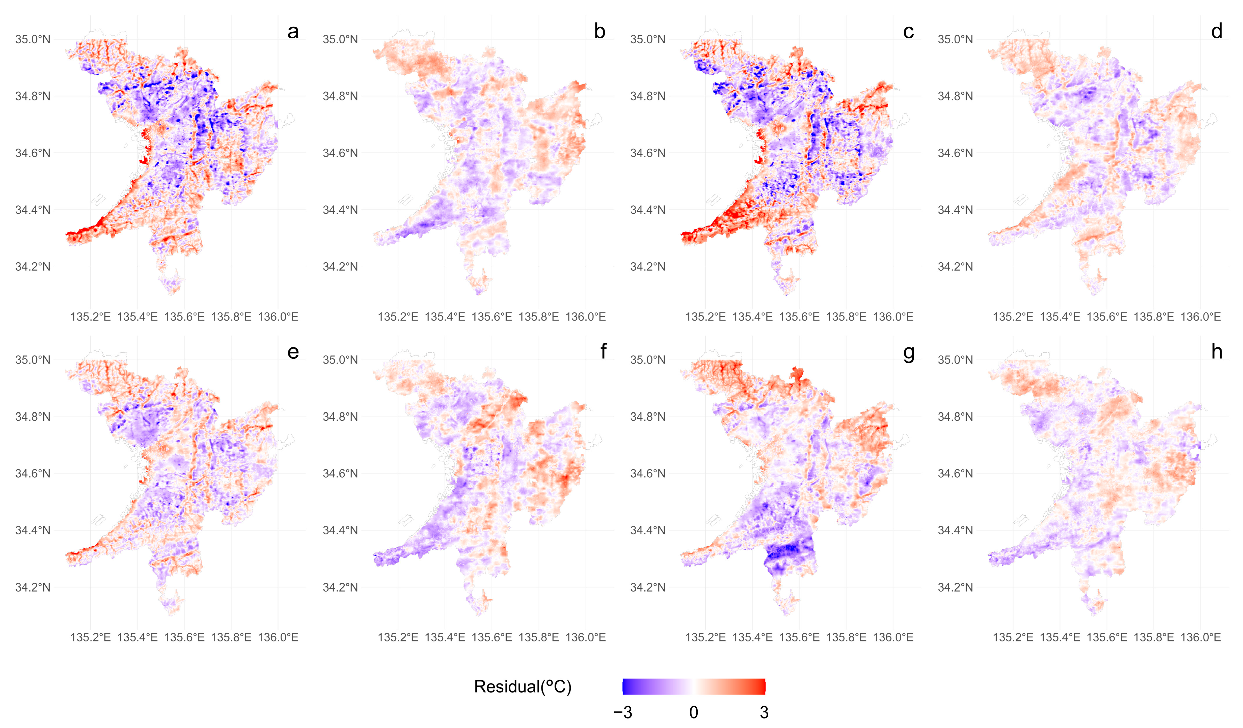
3.4. Estimation Error

To evaluate the estimation accuracy of the model, the residuals between estimated LSTs and observed ones (estimated value minus observed value of LST) are shown in Figure 10. Residuals are defined as the differences between the model’s estimated values and observed values. This figure indicates the existence of spatial correlation in the residuals.

During the daytime in spring and summer (Figure 10a,c), overestimation is observed in coastal and mountainous areas, while underestimation can be seen in the central region and the northern suburbs. In winter daytime (Figure 10g), overestimation is observed in the northern region, and underestimation is observed in the southern region. At night, spatial correlation is also observed, with the tendency being particularly pronounced in mountainous areas.

The primary focus in this estimation is on the analysis of the LST in urban areas, so data from non-urban areas were excluded from the model estimation. Mountainous areas have relatively few urbanized areas. This exclusion is considered one of the factors contributing to the errors observed in the mountainous areas. We also do not explicitly account for the effects of atmospheric stability, prevailing winds, and anthropogenic heat intensity. Mountainous areas and flat urban areas may exhibit different characteristics in terms of atmospheric stability and anthropogenic heat intensity. Building height could serve as a partial surrogate index for anthropogenic activities and their impact on surface temperature. The spatial autocorrelation of the errors suggests that the presence of uncontrolled factors in this study needs to be addressed.

4. Discussion

This study provides a comprehensive analysis of the seasonal and diurnal variations in the urban thermal environment of the Osaka Metropolitan Area. By integrating remote sensing data with statistical modeling, we have identified key urban morphology and environmental factors influencing LST. The findings reinforce the necessity of considering nonlinear interactions in UHI studies, as well as the benefits of advanced regression techniques in analyzing complex urban thermal patterns. To enhance the study’s contributions, this section further contextualizes the results within existing research and urban planning applications.

4.1. Policy Implications

The estimated model highlights the significant role of urban morphology, vegetation, and water surfaces in regulating the urban thermal environment. These findings suggest that urban planners should integrate targeted strategies to mitigate UHI effects, particularly in dense metropolitan areas.

Moreover, our results demonstrate that heat mitigation strategies should be tailored seasonally. For example, summer heat mitigation strategies should prioritize maximizing vegetative cover, while winter strategies should focus on balancing heat retention and dissipation in urban spaces. Additionally, local topography and microclimate conditions must be considered, as previous studies suggest that wind corridors and shading variations influence UHI intensity [3,33].

The findings confirm that building height significantly influences LST patterns, as presented in Section 3.2.1 and Section 3.3, summer exhibits the strongest overall influence of building height on temperature, driven by intense solar radiation and minimal shading; in contrast, winter shows the most distinct diurnal differences, with significant variations during the day but minimal changes at night; spring and fall display transitional patterns, with intermediate sensitivity influenced by moderate solar radiation, shadowing effects, and airflow dynamics. On the other hand, the scenario analysis in Section 3.3 demonstrates that the effects of building height vary both spatially and temporally. During the daytime, across all seasons, an increase in building height results in temperature reductions in central urban areas but leads to temperature increases in suburban areas. At night, however, an increase in building height consistently results in temperature increases across all locations. These results align with prior studies that demonstrate that taller buildings modify solar radiation exposure and airflow, contributing to local temperature variations [6,7]. Recent research also indicates that the optimization of urban geometry, including street orientation and building layout, can enhance heat dissipation and improve thermal comfort [24,25].

Additional studies highlight the role of the sky view factor (SVF) in mediating temperature fluctuations within high-rise environments, emphasizing the importance of urban morphology in shaping LST [34]. Our results suggest that high-rise developments should be carefully planned to balance shading benefits with ventilation pathways, ensuring that dense urban settings do not exacerbate nighttime heat retention. From these findings, it can be concluded that during the summer, promoting high-rise buildings in central areas while restricting building heights in suburban areas can help reduce temperatures. While these measures may lower temperatures during the winter as well, adjusting building heights seasonally is challenging, our results suggest that it is possible to optimize volumetric regulations considering thermal comfort throughout the year, as well as air conditioning energy consumption and other factors. Moreover, the analysis of building heights indicates that solar radiation conditions influence LST.

In addition to building height, factors such as façade reflectivity, shading devices attached to streets and buildings, and autonomous control like sunlight reflection control using mirrors and optical filters could be effective in improving the thermal environment. Quantifying these effects throughout the year could contribute to promoting strategies involving buildings and other structures in urban areas.

The cooling effects of vegetation, as measured by NDVI, reaffirm its importance in mitigating urban heat. However, our findings indicate that substantial cooling benefits occur only when vegetation surpasses a certain density threshold, demonstrated in Section 3.2.2, especially in summer. This aligns with earlier studies suggesting that urban greening initiatives must achieve critical coverage levels to be effective [12,13]. Additionally, mixed vegetation compositions (trees, shrubs, and grasses) have been shown to optimize temperature reductions, highlighting the need for diverse urban landscaping strategies [29].

Further research has shown that the cooling efficiency of vegetation depends on species selection and the spatial arrangement of green areas [36,37]. For instance, larger contiguous green spaces tend to offer stronger cooling effects than smaller fragmented ones. In highly urbanized settings, integrating vertical gardens and rooftop greenery may offer alternative pathways to increase vegetation density [39]. On the other hand, these measures to increase the vegetation intensity may lower temperatures during the winter as well. Considering the thermal environment, it is suggested that in the study area, green spaces be designed to feature a higher proportion of deciduous trees, ensuring that NDVI values are high in summer and low in winter. This approach could be an effective strategy in controlling the temperature throughout the seasons.

Deciduous trees are sometimes avoided as street trees due to the high costs associated with cleaning up fallen leaves. However, they can significantly improve the thermal environment, particularly enhancing pedestrian comfort, which in turn is expected to have various ripple effects on health, transportation, and other areas.

In the walkability context, evaluation methods of thermal environments considering seasonal differences have not been sufficiently studied. Although the spatial scale of our study is coarse to address the walkable environment directly, it can serve as a basis for understanding the impacts of seasonal and spatial thermal conditions.

Water bodies exhibit dual thermal effects, with daytime heat retention and nocturnal cooling. These patterns are consistent with research demonstrating that water features can amplify daytime UHI intensity while contributing to nighttime cooling [21]. However, variations in thermal effects due to water body size and surrounding land cover emphasize the need for integrated water-vegetation planning [40].

Previous studies suggest that water body thermal dynamics are influenced by depth and surrounding land surface material [41]. Deeper water bodies tend to retain heat longer, whereas shallow water bodies facilitate evaporative cooling more effectively. These insights reinforce the importance of integrating urban hydrology into planning frameworks to maximize cooling benefits [9].

4.2. Methodological Features and Limitations

In this study, the factors influencing seasonal and diurnal LST at the grid level were analyzed using a polynomial regression model. An elastic net was applied for the regularization of the model, and the model was selected based on the AIC. While most previous studies on LST factor analysis based on observations have assumed linear models [42], our study systematically addressed nonlinearity. This approach allowed for the estimation of models that adequately balance complexity and mitigate overfitting.

In recent years, machine learning models such as neural networks and random forests have been widely used to model phenomena with nonlinear mechanisms [9,29]. These methods have also advanced in incorporating regularization techniques, enabling the construction of models with strong generalization performance [9,29]. However, these machine learning models are typically characterized by a high degree of freedom, requiring empirical knowledge to determine model structures such as the number of layers or splits of trees. While these approaches offer high accuracy, they require extensive training data and parameter tuning. A direct comparison between these methods and the polynomial regression framework used in this study could provide further insights into their respective advantages and limitations.

There is room for further consideration regarding variable selection and model selection criteria. First, as seen in Figure 10, the model’s estimation errors exhibit spatial correlation, suggesting the potential influence of factors not included in this study. Terrain conditions such as slope and aspect, building density and land cover, and meteorological factors like sea breezes should also be considered. Moreover, anthropogenic heat emissions, wind patterns, and urban material properties could improve model robustness. Currently, it is difficult to find data with sufficient spatial and temporal resolution at the metropolitan scale. Furthermore, MODIS LST data limitations, particularly regarding the exclusion of large water bodies, may have influenced the observed temperature relationships. Future research should incorporate high-resolution thermal imaging and hydrological models to refine these findings. Criteria for model selection are another issue to be addressed. We used AIC for the criteria, but a large sample size usually results in a higher likelihood relative to the number of parameters, leading to the selection of more complex models. To address this issue, the Bayesian Information Criterion (BIC) or Minimum Description Length (MDL) should be compared with the results based on AIC.

By expanding variable selection, refining methodological approaches, and applying this framework to other metropolitan areas, future studies can enhance the generalizability and policy relevance of urban heat mitigation strategies. Additionally, incorporating real-time monitoring data and exploring hybrid modeling approaches that integrate physics-based simulations with statistical learning methods could further improve predictive accuracy [43].

The transferability of the proposed nonlinear model remains a crucial consideration for broader applications beyond the Osaka Metropolitan Area. While the model effectively captures regional thermal dynamics, its performance in other urban settings with varying climatic conditions, urban forms, and vegetation structures requires further validation. Differences in land cover characteristics, local microclimates, and anthropogenic heat contributions may impact model accuracy when applied to other cities. Future studies should focus on adapting and calibrating the model using datasets from diverse metropolitan regions to enhance its robustness and generalizability. Additionally, integrating high-resolution spatial datasets and localized climate variables could improve model adaptability, making it more applicable to urban heat island studies globally. Expanding its validation with independent datasets from different geographical contexts would further refine its predictive capacity and contribute to the development of scalable urban climate models.

Additionally, in the sensitivity analysis conducted in this study, during the daytime in spring, summer, and fall, wider water surfaces were associated with higher estimated temperatures. This result differs from previous studies [40,41]. In this study, water surfaces include not only rivers but also small ponds. Since LST is provided for land surface, large water bodies have missing data. Moreover, as water surfaces are often located in lowland areas and LST tends to be lower in higher-elevation mountainous regions, the data could be given the appearance of higher temperatures in areas with more water surfaces.

Although elevation is used as an explanatory variable, its influence might not have been sufficiently controlled. Further research is needed, including refining the selection method for the study area and combining insights from physical models that analyze urban thermal environments.

5. Conclusions

This study investigated the seasonal and diurnal variations in LST within the Osaka Metropolitan Area, emphasizing the impacts of urban morphology, vegetation, and water bodies. A key contribution is the use of polynomial regression with elastic net regularization, which successfully captures nonlinear interactions between urban features and temperature variations.

The results highlight that urban planning strategies must consider a combination of building height regulations, green infrastructure, and water management. Tall buildings contribute to both cooling and heat retention effects, necessitating careful zoning strategies. Vegetation coverage significantly mitigates LST, particularly when exceeding a critical density threshold, reinforcing the need for expansive greening initiatives, which would lead to colder temperatures in the winter season. Water bodies provide mixed effects, necessitating integrated planning to optimize their cooling potential while minimizing heat amplification.

Future research should incorporate high-resolution datasets, atmospheric factors, and socio-economic influences to further refine urban heat mitigation models. Expanding this framework to additional metropolitan areas will validate its broader applicability. Furthermore, investigating interactions between anthropogenic heat sources and urban design elements could enhance predictive modeling capabilities.

By bridging remote sensing, statistical modeling, and urban planning, this study provides valuable insights for policymakers seeking to develop climate-responsive strategies. The findings contribute to the broader discourse on sustainable urban development, emphasizing the necessity of multi-scale interventions to mitigate urban heat island effects and enhance thermal resilience in cities.