A Systematic Review of Machine Learning Algorithms for Soil Pollutant Detection Using Satellite Imagery

Abstract

Soil preservation from pollutants is essential for sustaining human and ecological health. This review explores the application of satellite imagery and machine learning (ML) techniques in detecting soil pollution, addressing recent advancements and key challenges in this field. Following the Preferred Reporting Items for Systematic Reviews and Meta-Analyses (PRISMA) guidelines, a comprehensive search across three major databases yielded 47 articles from an initial pool of 1018 publications spanning the last eight years. Among these, 34 studies focused on direct detection of soil pollutants, while 13 examined relationships between vegetation indicators and soil contaminants. This review evaluates various satellite platforms, highlights limitations of existing spaceborne sensors, and compares the effectiveness of ML models for soil pollution detection. Key challenges include the lack of standardization in datasets and methodologies, variations in evaluation metrics, and differences in algorithmic performance across studies. The findings emphasize the need for standardized frameworks and improved sensor capabilities to enhance detection accuracy. This work provides a foundation for future research, encouraging the integration of advanced ML models and multi-sensor satellite data for comprehensive soil pollution monitoring.

1. Introduction

Soil, a non-renewable resource and fundamental component of ecosystems, plays a vital role in supporting diverse ecological processes and sustaining life on Earth [1]. However, soil integrity is increasingly threatened by contaminants, including heavy metals, organic compounds from oil spills, and microplastics, which degrade soil quality and pose significant environmental and human health risks [2]. Contaminated soil can enter the human body through ingestion, inhalation, dermal contact, and indirect pathways, raising concerns about potential adverse health effects [3]. Soil pollution arises from both synthetic chemical introductions and natural alterations to soil properties [3]. Common sources of contamination include ruptured subsurface storage tanks, pesticide applications, surface water percolation, fuel and oil disposal, landfill leachate, and direct industrial discharge [3]. Among concerning pollutants are potentially harmful elements (PHEs), including heavy metals, semi-metals, and non-metals. These elements, like copper (Cu), lead (Pb), mercury (Hg), cadmium (Cd), and zinc (Zn), are naturally present at low levels due to weathering of the parent materials [4]. Under acidic soil conditions, PHEs can become soluble, impacting plants and contaminating groundwater [5]. Pollution by PHEs is particularly concerning in agricultural areas, where it threatens food security and environmental sustainability [6,7]. Alarmingly, approximately five million cases of soil contamination by metals or metalloids have been documented globally, affecting an estimated 506 million hectares of land [8].

Traditional soil sampling methods, which rely on discrete sampling, provide limited data points for constructing continuous maps of soil contamination, making it difficult to assess pollution levels over large geographic areas [9]. Laboratory analyses of soil samples, especially on a large scale, are time-intensive, costly, and environmentally burdensome [10]. Remote sensing technology, particularly visible and near-infrared reflectance (VNIR) spectroscopy, has thus emerged as a promising, scalable solution for cost-efficient monitoring of soil contamination [11].

The availability of satellite data and advancements in Graphics Processing Unit (GPU) capabilities [12] have enabled the application of deep learning methods, which outperform traditional machine learning models in various remote sensing tasks, including estimating precipitation, soil moisture, land surface and air temperature, crop yield, and pollutant detection [13,14,15]. Recurrent neural networks (RNNs) such as long short-term memory (LSTM), bidirectional long short-term memory (Bi-LSTM), and gated recurrent units (GRUs) have been developed to capture temporal relationships in time series data, showing promise for satellite-based evaluations [14,15].

Despite the expanding literature on soil pollution detection using satellite imagery, the field continues to evolve rapidly, driven by increasingly accessible and accurate satellite data. Several satellites, notably Sentinel-2 and Landsat 8, are frequently used for soil contamination studies [16]. A variety of machine learning methods have been applied, with Random Forest (RF) being the most popular, followed by techniques such as Cubist, Partial Least Squares Regression (PLSR), and Support Vector Machine (SVM) [17].

Evaluating detection results is critical in this field, with each study employing one or more metrics to assess model performance. Commonly used metrics include R-squared (R²), Root Mean Squared Error (RMSE), overall accuracy, F1 score, kappa statistics, and Ratio of Prediction to Deviation (RPD) [18].

In this evolving landscape of soil pollution detection, where advancements in machine learning (ML) and remote sensing drive progress, a review that consolidates existing evidence and insights is timely. While systematic reviews are common in life sciences, they are less frequently applied in earth and environmental sciences. This review synthesizes the literature on machine learning techniques for detecting soil pollutants through satellite imagery, offering new perspectives and insights into methodologies, data sources, and evaluation metrics. By conducting a rigorous analysis, this review not only bridges knowledge gaps but also advances the field of remote sensing technology for soil pollution monitoring. This study not only compiles key insights but also provides a new perspective to advance research in this field.

2. Materials and Methods

The methodology followed the PRISMA Extension Guidelines (PRISMA ScR [19,20,21]). A checklist is available in Figure 1, and the articles used to develop this checklist are listed in Appendix A. This section explains the Eligibility Criteria; Characteristics of the Accepted Studies (Participants, Detections Considered and Evaluated, and Study Design); Information Sources; Search Strategy; and additional data management and selection processes.

2.1. Eligibility Criteria: Search Characteristics

This systematic three-stage search approach ensured a comprehensive and focused collection of pertinent literature, enhancing the reliability and relevance of the research findings.

The review of soil pollution detection methods using satellite imagery and machine learning followed a structured, three-phase process. In the initial phase, a comprehensive search of the literature from 2016 to 2024 was conducted, using predefined keywords based on pertinent subject definitions. The search was limited to articles, cohort studies, case reports, and cross-sectional studies published in indexed journals in English drawn from 17 peer-reviewed journals.

In the second phase, articles were meticulously selected based on eligibility criteria to ensure alignment with the research objectives. Only those meeting all criteria were advanced for further analysis. In the final phase, abstracts of the selected articles were reviewed to assess relevance to the research topic, including only those closely aligned with the study focus. This review approach ensured a comprehensive, relevant collection of the literature.

2.2. Characteristics of the Accepted Studies

2.2.1. Participants

The investigation for relevant research in the field of machine learning applied to soil contaminants was performed without imposing any specific restrictions on the type of contaminants or soil types. The search encompassed studies that employed machine learning algorithms on various types of satellite images.

The inclusion criteria were deliberately broad to ensure a comprehensive representation of the research in this domain. Consequently, all studies involving machine learning techniques on soil contaminants, regardless of the specific contaminants involved or the type of soil, were considered.

Furthermore, studies utilizing diverse satellite images and employing various machine learning algorithms were included in the search. This approach aimed to encompass the broad spectrum of methodologies employed in this field, providing a comprehensive and diverse collection of studies for analysis.

By adopting an inclusive approach to participant selection and study characteristics, this research ensures a comprehensive and well-rounded exploration of machine learning applications on soil contaminants using satellite imagery.

2.2.2. Detections Considered and Evaluated

The study focused on the following detection categories:

• Assessment of satellite imagery: Analysis of images captured by satellites.
• Machine learning methodologies: Evaluation of machine learning techniques used for satellite image analysis.
• Identification of contaminated soil types: Detection and assessment of contamination types through analysis described in (B), evaluated by (A).
• Validation of results: Verification of identified contaminated soil types (C) by comparing with on-ground sampling data.

By evaluating these categories, the study aimed to provide a comprehensive understanding of machine learning applications for soil contaminants.

2.2.3. Design of Accepted Studies

The design of accepted studies focused on specific criteria, including the use of satellite images, computational analysis, and image processing to assess soil characteristics. The objective was to develop models with minimal error and high accuracy, enabling generalization to various locations and contaminations. Notably, contaminants included heavy metals; chemicals; and soil-related features like moisture, erosion, salinity, and evaporation. Studies using images from aircraft or drones were excluded to emphasize the unique advantages of satellite imagery in soil characterization and pollution detection.

2.3. Information Sources

Data were collected from key digital databases, including ScienceDirect, Scopus, and Web of Science. Filters applied within each database included publication year (2016–2024), document type (articles and articles in press), and language (English). Only scholarly journal articles and scientific publications were considered.

2.4. Search Strategy

The search strategy comprised the amalgamation of the subsequent keywords: “machine learning”, “deep learning”, “artificial intelligence”, “polluta*”, “contamina*”, satellite, algorithm, image, and soil.

Consequently, thirteen combinations were deemed valid:

• “Machine learning” AND polluta* AND satellite;
• “Deep learning” AND polluta* AND satellite;
• “Artificial intelligence” AND polluta* AND satellite;
• “Machine learning” AND polluta* AND image AND soil;
• “Deep learning” AND polluta* AND image AND soil;
• “Artificial intelligence” AND polluta* AND image AND soil;
• “Machine learning” AND polluta* AND Algorithm AND satellite;
• “Machine learning” AND soil contamina* AND satellite;
• “Deep learning” AND contamina* AND Satellite AND soil;
• “Artificial intelligence” AND soil contamina* AND satellite;
• “Machine learning” AND soil AND contamina* AND image;
• “Deep learning” AND contamina* AND image AND soil;
• “Artificial intelligence” AND soil AND contamina* AND image.

2.5. Study Records

2.5.1. Data Management

To ensure systematic data handling, relevant studies were sourced from academic databases and archived using Mendeley Reference Manager (version 2.131.0), facilitating structured organization and seamless retrieval. Extracted data were systematically recorded in an Excel database, where each row represented an individual study, and each column captured key study parameters. This structured approach ensured accuracy in data compilation and facilitated a detailed analysis of the research findings.

2.5.2. Selection Process

The selection process involved multiple phases to ensure the inclusion of relevant and eligible studies for the review. Initially, records were automatically screened based on predefined criteria, including publication year (2016–2024, to align with the PRISMA method’s focus on recent literature), document type (articles and forthcoming articles), source type (peer-reviewed journals), and language (English). This automated screening helped narrow the pool of potential studies.

Next, a researcher conducted a manual review to assess each work’s alignment with the research objectives, based solely on screening titles and abstracts. Any records with uncertain relevance after this initial verification proceeded to the next selection phase.

In the second screening stage, the methodologies used in each study were evaluated against the eligibility criteria, requiring a comprehensive reading of each article. Studies accepted for inclusion met all of the following minimum criteria:

• Utilization of artificial intelligence techniques, such as machine learning (ML) and deep learning (DL), for image processing.
• Detection of soil pollutants or soil characteristics related to soil pollutants, such as soil evaporation or soil moisture content.
• Exclusive use of satellite images (excluding airborne or drone data and soil testing data) for analysis.
• Validation of data through methods that measure accuracy or error in detecting soil pollutants, such as field soil testing.
• Description and specification of the machine learning methods used for image processing, especially if developed by the author.
• Defined accuracy metrics and presentation of results in quantifiable terms.

By adhering to these stringent selection criteria, this study ensured the inclusion of works that met the research objectives and contributed to a comprehensive analysis of artificial intelligence applications in soil pollutant detection using satellite imagery.

2.6. Data Collection Process

During data collection, the results of each study were presented in a detailed description using a table format. Both the results and conclusions were carefully analyzed, focusing on content with potential causal links to the objectives of the systematic review.

The information extracted and included in Appendix A comprises the following key elements:

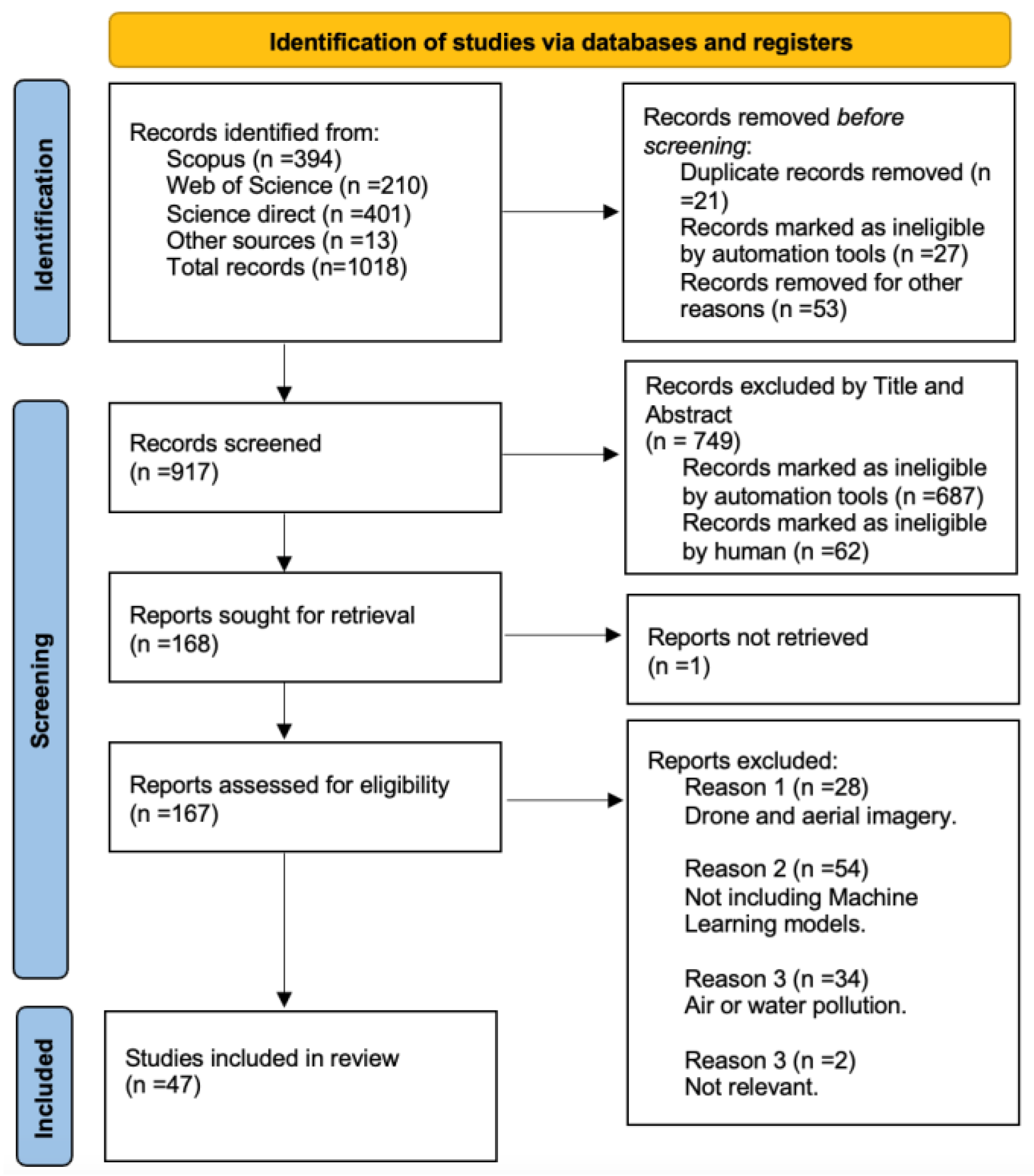
• References: Each article reference is provided. Following a meticulous review of over 1000 articles using the PRISMA method, a final selection of 36 articles was made to align with the specific goals of this review. Further details on these selected articles are presented in the accompanying table.
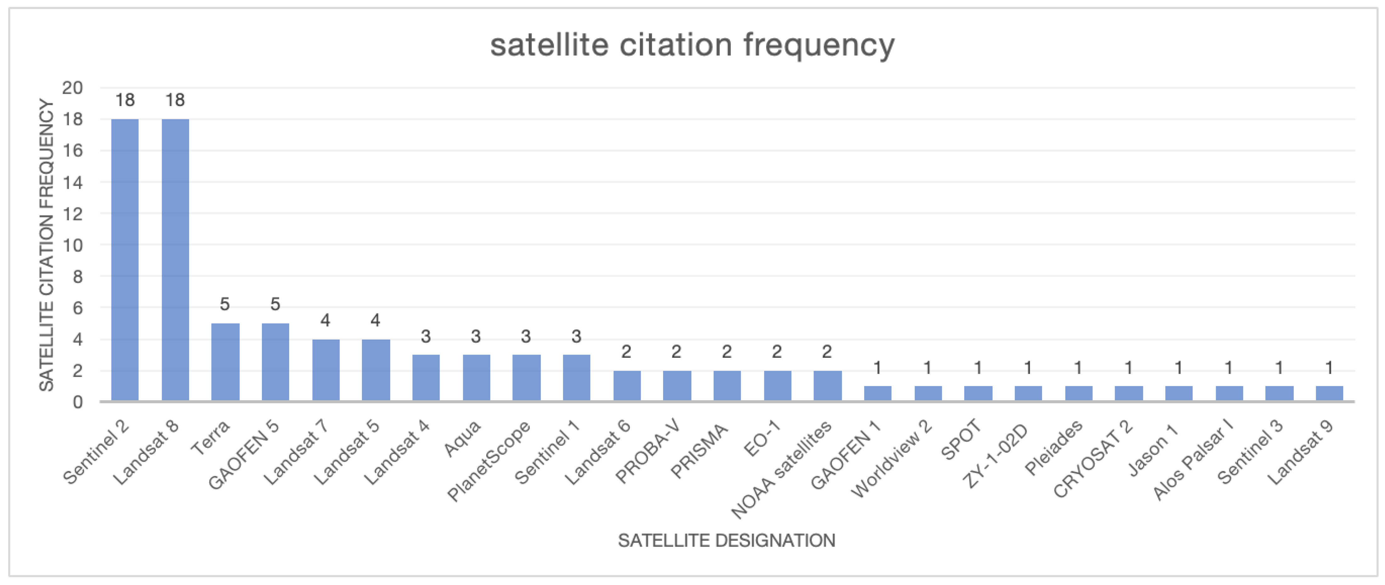
• Satellite Name: The appendix’s second column lists the satellites used in each article, with some studies focusing on imagery from a single satellite while most compare multiple satellites. This approach aids in selecting the most suitable satellite(s) for specific applications.
• Machine Learning Methods: The types of machine learning (ML) techniques employed by the authors and any unique methodologies they developed.
• Contaminant Types: A list of all contaminants or pollutants studied, as well as other soil characteristics related to soil pollutants. The names of these parameters are presented in the fourth column of the appendix.
• Validation: Validation of each ML method is a critical aspect, evaluating the effectiveness of the techniques for interpreting satellite images. Typically, this validation involves direct soil sampling at specified depths, ensuring an understanding of the correlation between soil samples and satellite imagery. The number of boreholes used varies with the investigated area, as indicated in the appendix.
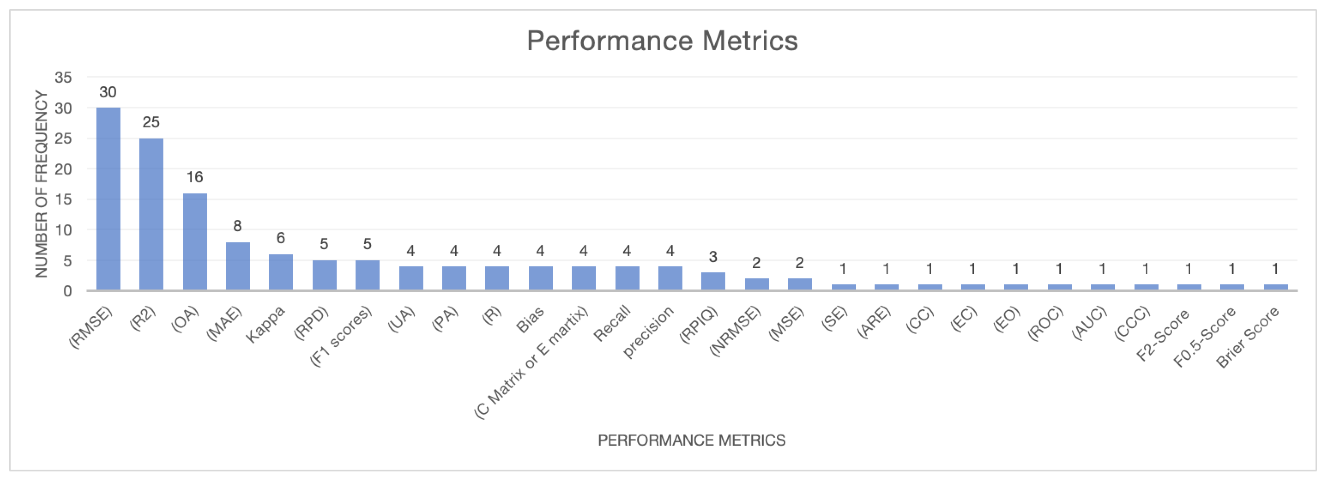
• Performance: Machine learning performance metrics serve as quantitative measures to assess model accuracy and effectiveness across classification, regression, or clustering tasks. Each article’s specific performance metrics and the best results are summarized in a table or presented as final values in the appendix.
• Results: The last column of Appendix A provides a concise conclusion for each article, showing how each study’s results align with the systematic review’s purpose. This section facilitates an understanding of the effectiveness of different methods, satellite types, and other parameters for pollution detection.

By systematically gathering and organizing this comprehensive data, the review enabled an in-depth analysis and drew meaningful conclusions on the application of machine learning for soil pollutant detection using satellite imagery.

2.7. Prioritization and Outcomes

Quantitative Prioritization:

• Validation Sample Size: Studies using larger sample sizes for validation were given higher priority. Substantial sample sizes enhance the statistical robustness and reliability of findings, improving the overall quality of the research.
• Accuracy of Validation Data: Articles that employed the most accurate and reliable validation methods for analyzing images through machine learning were prioritized. High-quality validation data add credibility to research outcomes and strengthen confidence in the reported results.

Qualitative Prioritization:

• Identification of Different Contaminations: Studies that directly identified various contaminations or indirectly inferred them through specific soil characteristics were considered more significant. This approach broadens the research scope, providing insights into a diverse range of soil pollutants and their potential impacts.
• Diverse ML Methods: Articles exploring various machine learning methods for image analysis were prioritized. Employing diverse ML methodologies enables a comprehensive exploration of soil pollutant detection approaches, enhancing the understanding of their effectiveness.

By employing this comprehensive prioritization approach, the review aimed to highlight studies with strong methodological rigor, broad scope, and substantial potential to provide valuable insights into the use of machine learning for soil pollutant detection using satellite imagery.

2.8. The Risk of Bias and Quality Assessment

To evaluate the reliability of the included studies, a risk of bias assessment was conducted using established methodological and data analysis parameters (see

Table 1. Bias analysis of each study.

Study	Different Satellite Sources	ML Methodology Variation	Variation of Detected Contaminant	Performance Analysis Alteration	Sampling Quantity	Sampling Quality	Validation Data
[22]	LR	HR	LR	LR	LR	LR	LR
[23]	LR	LR	UR	HR	LR	LR	LR
[24]	HR	HR	LR	LR	UR	UR	LR
[25]	HR	LR	HR	LR	UR	LR	LR
[26]	LR	HR	UR	LR	LR	LR	LR
[27]	HR	HR	UR	LR	UR	HR	LR
[28]	HR	LR	LR	LR	LR	LR	LR
[29]	LR	LR	UR	LR	HR	LR	LR
[30]	HR	LR	UR	UR	LR	LR	LR
[31]	LR	LR	HR	LR	LR	LR	LR
[32]	HR	HR	UR	LR	HR	LR	LR
[33]	HR	LR	HR	LR	LR	LR	LR
[34]	HR	HR	UR	UR	HR	LR	UR
[35]	HR	LR	UR	LR	LR	LR	LR
[36]	HR	LR	HR	LR	LR	LR	LR
[37]	HR	LR	LR	LR	LR	LR	LR
[38]	HR	LR	LR	LR	LR	LR	LR
[39]	LR	LR	LR	LR	LR	LR	LR
[40]	HR	HR	UR	UR	UR	UR	LR
[41]	HR	HR	UR	HR	HR	LR	LR
[42]	HR	LR	LR	LR	LR	LR	LR
[43]	LR	HR	LR	HR	HR	LR	LR
[44]	HR	LR	UR	LR	LR	LR	LR
[45]	LR	LR	LR	LR	LR	LR	LR
[46]	LR	LR	LR	LR	LR	LR	LR
[47]	HR	LR	LR	HR	LR	LR	LR
[48]	LR	HR	UR	LR	LR	LR	LR
[49]	HR	LR	HR	LR	HR	LR	LR
[50]	HR	LR	UR	LR	LR	LR	LR
[51]	LR	LR	UR	LR	UR	LR	LR
[52]	LR	HR	UR	LR	UR	LR	LR
[53]	LR	HR	UR	HR	LR	LR	LR
[54]	LR	HR	UR	LR	HR	LR	LR
[55]	LR	HR	UR	LR	LR	LR	LR
[56]	LR	LR	HR	LR	LR	LR	LR
[57]	HR	LR	LR	LR	LR	LR	LR

HR: high risk; LR: low risk; UR: unclear risk.

). These parameters were categorized based on their potential impact on study outcomes, classified as “high risk”, “low risk”, or “unclear risk”:

• Satellite Source Diversity: Evaluated the range and types of satellite data utilized.
• Machine Learning Methodology Variation: Assessed differences in ML approaches across studies.
• Contaminant Diversity: Examined the range of pollutants detected.
• Performance Analysis Methods: Investigated the metrics and validation techniques used.
• Sampling Quantity and Quality: Considered the number and reliability of samples used for model training and validation.
• Validation Data: Assessed the rigor of the accuracy measurement methods.

This assessment ensured that biases in data sources, methodological variability, and validation techniques were critically examined, enhancing the robustness of this review’s findings.

With the exception of sampling quality and quantity, all other variables in the methodology section emphasize the need for improved reporting regarding variation and validation of results.

2.9. Article Selection

Following PRISMA guidelines [58], the initial database searches yielded 1018 items. After removing duplicates and ineligible entries using automated tools and other criteria, 917 records remained for further consideration. During the screening process, 749 records were excluded based on title and abstract ineligibility, identified through a combination of automated and manual assessment. Additional exclusions were made for studies involving drone and aerial imagery, lacking machine learning models, or unrelated to soil pollution, resulting in a final selection of 47 articles for detailed review. Figure 1 provides an overview of the number of articles identified at each step, following the PRISMA methodology.

Figure 1. PRISMA flow diagram of the research [19].

Figure 1. PRISMA flow diagram of the research [19].

3. Results, Discussion, and Summary of Evidence

This section presents the culmination of a systematic review exploring the advancements in satellite-based soil contaminant detection. The investigation leverages satellite imagery and includes the selection and analysis of relevant studies employing state-of-the-art machine learning methodologies. Through meticulous screening and evaluation, the efficacy of satellite systems in detecting diverse soil pollutants and characteristics is revealed. Emphasizing cost-effectiveness, accessibility, and accuracy, this review highlights the transformative potential of satellite-based methods in soil pollution monitoring and management.

Satellite imagery has emerged as an effective method for soil contaminant detection, offering advantages in cost, accessibility, and accuracy. In the pursuit of identifying soil contaminants, researchers have utilized data from several satellites, often incorporating images from multiple sources in their studies, as illustrated in Figure 2. Among the most widely used satellites, Sentinel-2 [22,26,30,31,38,41,43,47,51,52,54,55,56,57,59,60,61] and Landsat 8 [22,24,25,27,31,38,41,44,45,51,53,54,55,56,62,63,64,65] stand out, with each appearing frequently in the literature. These satellites, integral to distinct Earth observation systems, have been applied across various domains, including land use mapping, environmental monitoring, and natural resource management. Specifically, seven studies used Sentinel-2 for soil property detection [31,47,51,52,54,55,56] and four studies employed it for heavy metal detection [14,31,47,52]. Additionally, five studies utilized Sentinel-2 for vegetation property assessment [30,41,59,60,61].

For Landsat 8, seven studies focused on heavy metal detection [25,42,44,45,56,63,64], another seven on soil property detection [31,51,53,54,62,65,66], and one study assessed vegetation properties [27]. Sentinel-2, part of the Copernicus Programme developed by the European Space Agency (ESA), provides high-resolution, multispectral images of the Earth’s surface. Equipped with a multi-spectral imaging instrument that captures data in 13 spectral bands—from visible to shortwave infrared—the satellite achieves a spatial resolution between 10 to 60 m and covers the Earth’s land surface every five days [49,67].

Landsat 8, developed through the collaborative efforts of NASA and the United States Geological Survey (USGS) under the Landsat program, is equipped with two instruments: the Operational Land Imager (OLI) and the Thermal Infrared Sensor (TIRS). OLI captures data in nine spectral bands, covering the visible to shortwave infrared spectrum, with a spatial resolution ranging from 15 to 100 m. TIRS captures data in two thermal infrared bands with a 100-m resolution, providing comprehensive global land coverage every 16 days [68].

Nearly 40% of the reviewed articles (18 out of 47) utilized multiple satellites, allowing comparisons across satellite systems and creating a robust dataset for analysis [22,23,26,31,35,39,43,45,47,51,52,53,54,55,56,59,60,64]. This multi-satellite approach enhances data reliability and enables a more comprehensive analysis of soil contaminants. By combining data from different satellite sources, researchers can address limitations inherent to individual satellite systems, such as temporal resolution and spectral range, thereby improving overall accuracy and analytical depth.

In summary, the use of satellite imagery for soil contaminant detection is increasingly validated by a growing body of literature. The integration of multiple satellite datasets and advanced machine learning techniques holds significant potential for improving soil pollution monitoring and management. As technology advances and more sophisticated satellites are launched, the precision and applicability of these methods are expected to enhance further, paving the way for more effective environmental conservation strategies.

The analysis of machine learning (ML) methods for soil contaminant detection reveals distinct patterns and preferences. The most frequently used methods are decision tree-based models, as illustrated in Figure 3 and

Table 2. Frequency of machine learning methods used in the references.

Method of Machine Learning	Number of Frequency
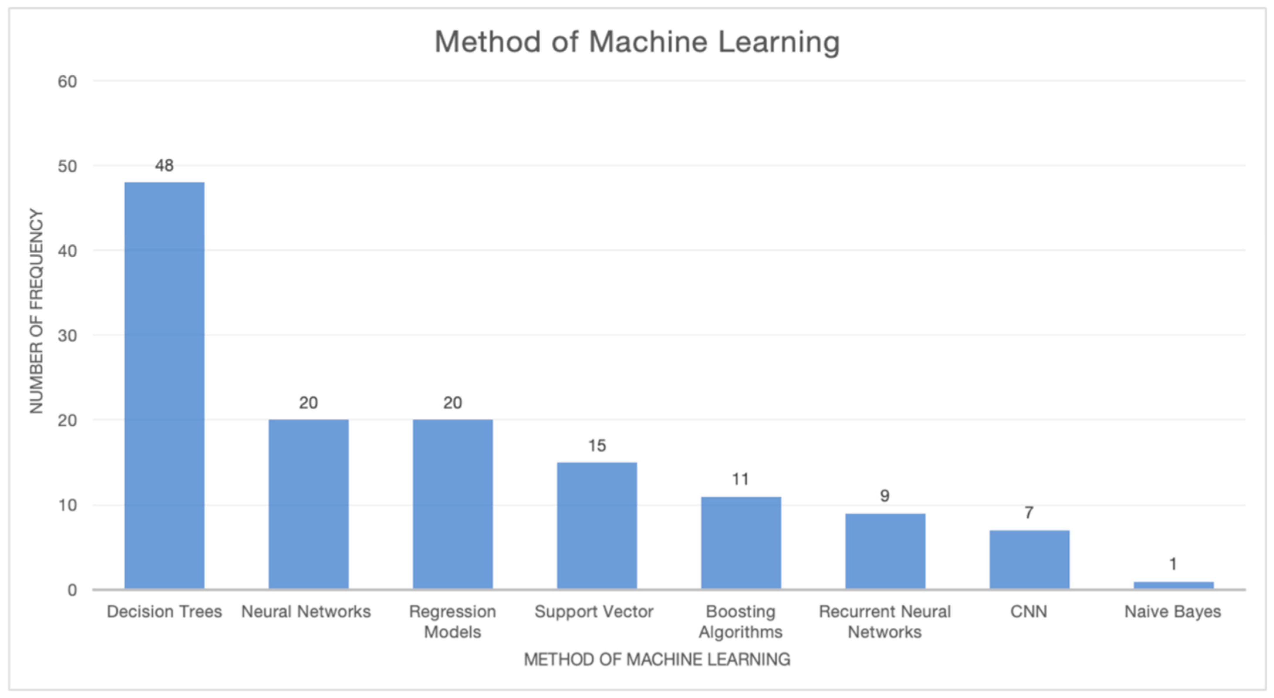
Decision Trees (Random Forest (RF), ExtraTrees (ET), Decision Tree, Cubist (Cu), Classification and Regression Trees (CART), Deep Forest Algorithm)	48
Neural Networks (Artificial Neural Network (ANN), Backward Propagation Neural Network (BPNN), The general regression neural network (GRNN), Patch-based multi-image NN system (Patch multi), Patch-based single-image NN system (Patch Single), Pixel-based multi-image NN system (Pix multi), Pixel-based single-image NN system (Pix single), Multi-Layer Perceptron (MLP), Extreme Learning Machine (ELM))	20
Regression Models (Partial Least Squares Regression (PLSR), K Nearest Neighbor (KNN), Gaussian Process Regression (GPR), Generalized Linear Models (GLMs), Geographically Weighted Regression (GWR), kernel ridge regression (KRR), Linear Regression Model, Stepwise Multiple Linear Regression (SMLR), Multiple Linear Regression (MLR))	20
Support Vector (Support Vector Machine (SVM), support vector regression (SVR))	15
Boosting Algorithms (Gradient Descent Boosting Trees (GDB), Adaptive Boosting (ADB), eXtreme Gradient Boosting (XGB), Generalized Boosting Methods (GBMs))	11
Recurrent Neural Networks (RNNs) (Long short-term memory (LSTM), Bidirectional LSTM (Bi-LSTM), Gated Recurrent Unit (GRU), Pixel-based RNN system (Pix RNN), Proposed patch-based RNN (PB-RNN))	9
Convolutional Neural Network (CNN)	7
Naive Bayes	1

, including Random Forest (RF), ExtraTrees (ET), Decision Tree, Cubist (Cu), Classification and Regression Trees (CART), and the Deep Forest Algorithm. Among these, Random Forest emerges as the most prevalent, with 33 instances in the literature [12,28,31,32,33,34,35,36,37,38,39,40,41,42,43,44,45,46,47,48,49,50,59,60,61,62,63,64,65,66,69,70]. This preference underscores the robustness and effectiveness of Random Forest in handling the complexities of soil contaminant detection.

Random Forest is well regarded for its proficiency in land cover classification and feature extraction. Studies have applied RF to classify land cover types from Sentinel-2 imagery, achieving an overall accuracy of 83% [41]. Similarly, Chen et al. used RF to extract urban green spaces from Landsat 8 imagery, obtaining an accuracy of 89.15% [34]. RF’s strengths in satellite image processing include its ability to handle large datasets with high-dimensional features and robustness in managing noise and outliers. Additionally, the model allows for feature importance analysis, which aids in identifying crucial variables for classification and feature extraction tasks [36].

Following Random Forest, other frequently used methods include Support Vector Machine (SVM) with 10 instances [29,30,37,39,46,49,57,60,66,70], Cubist with 6 instances [28,42,45,48,50,55], and both Artificial Neural Network (ANN) and Partial Least Squares Regression (PLSR) with 6 instances each [14,33,34,40,58,69].

SVM, a versatile supervised learning algorithm, is commonly used for classification and regression. It works by finding an optimal hyperplane that separates data classes. SVM has been successfully applied in remote sensing and image analysis, achieving reliable classification results based on satellite imagery [28,42]. Its versatility and ability to handle complex datasets make SVM valuable in soil contaminant detection [48].

Other methods include KNN [28,37,47,49,60], BPNN [38,46,49], CART [30,37,47], CNN [34,39,43,59,62], MLP [37,49,59,65], ADB [33,37], ELM [31,46,62], LSTM [23,43,70], Pix RNN [27], [43], and SVR [25,28,60]. The varied frequency of these methods reflects a diverse approach to satellite imagery analysis for soil contaminant detection, with each method contributing unique strengths and capabilities.

Additionally, 56% (32 out of 57) of the reviewed articles used multiple ML models to compare and validate datasets, which allowed researchers to identify the most effective model for specific environmental parameters [23,25,27,28,29,30,31,33,35,36,37,38,39,42,43,44,45,46,47,48,49,50,51,56,59,60,62,63,65,66,69,70]. The results showed that Random Forest was most often (13 of 32 instances) identified as the best model [29,33,36,38,39,42,44,45,46,47,50,60,63], while SVR and ANN each achieved the best results three times.

The reliance on Random Forest illustrates its robustness and reliability in soil contaminant detection. The diversity of other methods highlights the tailored approaches researchers adopt to address specific challenges. As ML techniques advance and integrate with new satellite technologies, the accuracy and applicability of these methods are expected to improve, enhancing soil contamination monitoring and environmental management.

Evaluating detection results is crucial in this research, with each article employing one or more evaluation metrics. Among the selected studies, 30 used Root Mean Squared Error (RMSE) [23,25,28,29,31,33,35,36,37,42,45,46,48,49,50,51,52,54,55,56,57,60,61,63,64,65,69,70], a metric that measures the average difference between predicted and actual values. For instance, Ma and Liang [23] used RMSE to evaluate a deep learning model for image super-resolution, achieving an RMSE of 9% on the Actin validation set [70].

The equation of Root Mean Squared Error (RMSE) is as follows:

$$\mathrm{R}\mathrm{M}\mathrm{S}\mathrm{E}=\sqrt{{\sum }_{\mathrm{i}=1}^{\mathrm{n}}{\displaystyle \frac{{\left({\mathrm{y}}_{\mathrm{i}}-{\mathrm{y}}_{\mathrm{p}}\right)}^2}{\mathrm{n}}}},$$

(1)

where y_i represents the actual (observed) value of the target variable for data point i, and y_p represents the predicted value of the target variable for data point i.

In addition to RMSE, 25 articles used the coefficient of determination (R²) [22,23,25,28,29,31,35,36,37,38,42,46,48,49,50,51,54,55,56,60,61,62,63,64,65,69], indicating how well the model fits the data. The equation of the coefficient of determination (R²) is given by

$${\mathrm{R}}^2=1-{\displaystyle \frac{\sum {\left({\mathrm{y}}_{\mathrm{i}}-{\mathrm{y}}_{\mathrm{p}}\right)}^2}{\sum {\left({\mathrm{y}}_{\mathrm{i}}-\overline{\mathrm{y}}\right)}^2}},$$

(2)

where $\overline{\mathrm{y}}$ is the mean of the actual values.

Moreover, 16 articles reported overall accuracy (OA) as a key performance metric accuracy [26,27,29,30,36,39,41,43,44,47,49,53,59,62]. OA is calculated using the equation

$$\mathrm{O}\mathrm{A}={\displaystyle \frac{\mathrm{T}\mathrm{P}+\mathrm{T}\mathrm{N}}{\mathrm{T}\mathrm{P}+\mathrm{T}\mathrm{N}+\mathrm{F}\mathrm{P}+\mathrm{F}\mathrm{N}}},$$

(3)

where TP and TN represent correctly classified instances, and FP and FN denote misclassified cases. Additionally, the Mean Absolute Error (MAE) was reported in five studies [22,25,28,33,46]. MAE is a common regression metric that quantifies the absolute differences between predicted and observed values:

$$\mathrm{R}\mathrm{M}\mathrm{S}\mathrm{E}={\displaystyle \frac{1}{\mathrm{n}}}{\sum }_{\mathrm{i}=1}^{\mathrm{n}}\left|{\mathrm{y}}_{\mathrm{i}}-{\mathrm{y}}_{\mathrm{p}}\right|,$$

(4)

where y_i represents the actual (observed) value of the target variable for data point i, and y_p represents the predicted value of the target variable for data point i. Furthermore, Ratio of Prediction to Deviation (RPD) was reported in five studies [37,38,55,56,57]. RPD is an important metric for evaluating predictive models in environmental sciences and is computed as

$$\mathrm{R}\mathrm{P}\mathrm{D}={\displaystyle \frac{\mathrm{S}\mathrm{D}}{\mathrm{R}\mathrm{M}\mathrm{S}\mathrm{E}}}$$

(5)

where SD is the standard deviation of measured values, and RMSE is the Root Mean Squared Error. A higher RPD value typically indicates a more reliable and accurate model. These metrics collectively provide a comprehensive assessment of model performance, covering both classification and regression-based evaluations (Figure 4).

The primary objective of this study was to identify environmental parameters associated with soil pollution, both directly and indirectly. Notably, vegetation properties were linked to specific types of pollution, impacting various vegetation types [32]. Among the parameters examined, heavy metals played a crucial role, focusing on copper (Cu), arsenic (As), cadmium (Cd), chromium (Cr), nickel (Ni), lead (Pb), zinc (Zn), and iron (Fe). These metals were assessed based on three core factors: gravity, toxicity, and mobility. The gravity factor referred to the extent and concentration of heavy metal contamination in the soil, while the toxicity factor measured harmful effects on human health, plants, and animals. The mobility factor gauged each metal’s potential to migrate from soil to other environmental compartments, such as groundwater or surface water, potentially causing contamination in these areas [71].

Figure 5 shows that heavy metals were the most frequently studied environmental parameters, with a frequency count of 47, substantially higher than other pollutants. Specifically, copper (Cu) was examined [25,37,42,44,45,46,63,69], chromium (Cr) six times [22,28,37,44,45,63], iron (Fe) six times [22,28,38,42,44], arsenic (As) seven times [33,37,44,45,49,63,69] nickel (Ni) appeared five times [42,44,45,46,63], zinc (Zn) six times [22,28,36,44,46,63,69], lead (Pb) six times [28,38,45,63,64,69], and cadmium (Cd) two times [38,44]. Following heavy metals, soil characteristics were the second most frequently studied environmental parameter, appearing 15 times. These characteristics included soil organic carbon, soil organic matter (SOM), surface soil moisture, soil loss, soil erosion, soil texture, clay content, soil pH, soil salinity, and evaporation [29,31,32,35,38,40,44,47,48,50,52,53,54,55,57].

Plastic pollution, including microplastics and various plastic materials such as polyethylene (PE), polypropylene (PP), polyvinyl chloride (PVC), polyethylene terephthalate (PET), polystyrene (PS), acrylonitrile butadiene styrene (ABS), ethylene vinyl acetate (EVA), polyamide (PA), polycarbonate (PC), and polymethyl methacrylate (PMMA), ranked third in frequency in the selected articles, appearing 11 times [34,39]. These findings underscore the significance of heavy metals and soil characteristics in soil pollution studies, as well as the rising concern over plastic pollution and its environmental impact.

Satellite images have been instrumental in detecting direct and indirect indicators of soil pollutants across studies. As shown in

Table 3. Detailed detection of the environmental parameters.

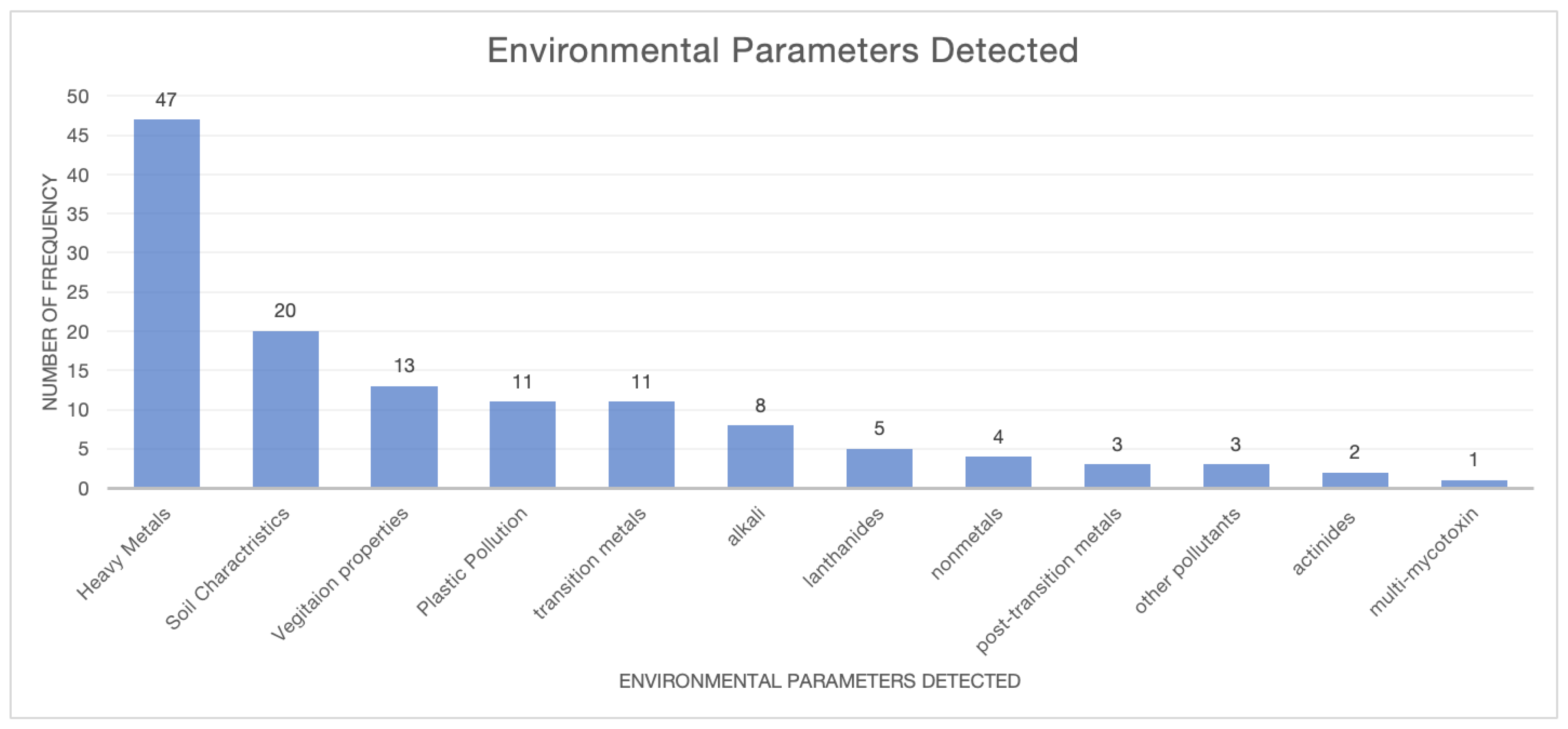
Environmental Parameters Detected	Number of Frequencies
Heavy Metals including (copper (Cu), arsenic (As), cadmium (Cd), chromium (Cr), nickel (Ni), lead (Pb), zinc (Zn), iron (Fe))	47
Soil Characteristics including (soil organic carbon, soil organic matter (SOM), surface soil moisture, soil loss, soil erosion, soil texture, clay content, soil pH, soil salinity, evaporation, soil fauna, soil microbes, electrical conductivity (EC), calcium carbonate equivalent (CCE))	20
Vegetation Properties including (land cover, leaf area index (LAI), cropland suitability assessment, crop productivity, tree counting)	13
Plastic Pollution including (microplastics pollution, plastics polyethylene (PE), polypropylene (PP), polyvinyl chloride (PVC), polyethylene terephthalate (PET), polystyrene (PS), acrylonitrile butadiene styrene (ABS), ethylene vinyl acetate (EVA), polyamide (PA), polycarbonate (PC), polymethyl methacrylate (PMMA))	11
Transition Metals including (Ti (titanium), V (vanadium), Cr (chromium), Mn (manganese), Fe (iron), Co (cobalt), Cu (copper), Zr (zirconium), Nb (niobium), Mo (molybdenum), Cd (cadmium), Hf (hafnium), W (tungsten), M (molybdenum))	11
Alkali and Alkaline Earth Metals including (Na (sodium), Mg (magnesium), K (potassium), Ca (calcium), Sr (strontium), Ba (barium), Cs (cesium))	8
Lanthanides or Rare Earth Elements including (Ce (cerium), Pr (praseodymium), Nd (neodymium), Y (yttrium), La (lanthanum))	5
Nonmetals including (Si (silicon), P (phosphorus), S (sulfur), Br (bromine))	4
Post-Transition Metals including (aluminum (Al), gallium (Ga))	3
Actinides including (Th (thorium), U (uranium))	3
Other pollutants (oil spill, dust and its sources, pollution by urban influence on Inland Marsh)	3
Multi-mycotoxin contamination (such as deoxynivalenol and zearalenone)	2

, heavy metals were directly identified in 34 articles through satellite imagery, while 15 articles focused on detecting a range of soil parameters, including soil organic carbon, SOM, surface soil moisture, soil loss, soil erosion, soil texture, clay content, soil pH, soil salinity, and evaporation.

Additionally, plastic pollution, which encompasses microplastics and specific plastic types such as PE, PP, PVC, PET, PS, ABS, EVA, PA, PC, and PMMA, is also detectable through satellite imagery. Vegetation properties, including land cover, leaf area index (LAI), cropland suitability, and crop productivity, have emerged as indicators of soil pollutants when analyzed using satellite data. This comprehensive overview highlights the diverse range of environmental parameters that satellite technology can effectively monitor for soil pollution assessment and identification.

The number of samples used for validation is crucial in machine learning applications, as a higher number of samples enhances the accuracy of data extraction from satellite imagery. However, the specific number of samples required can vary depending on factors such as task complexity, data diversity, and model architecture. To prevent overfitting and reduce errors, an appropriate range of samples is typically defined during the programming phase. Among the selected articles, 34 studies utilized soil samples for validation [22,23,25,26,28,29,30,31,32,33,34,35,36,37,38,39,42,43,44,45,46,47,48,49,50,54,55,57,59,61,63,64,65,69].

The number of samples varied significantly across studies, ranging from as few as 6 cases to as many as 15,188 cases. This variation is influenced by factors such as the geographic extent of the study area, data accessibility, and sampling feasibility. Among the 28 articles mentioned, 24 studies evaluated more than one hundred samples, indicating a robust validation process [22,25,26,28,29,30,31,35,36,38,39,42,45,46,47,48,50,56,57].

Given that satellite imagery primarily detects surface soils, the sampling depth is another critical factor in soil contaminant studies. Sampling depth provides essential insights into the distribution of soil contaminants. In the reviewed articles, 13 studies specified sampling depths, ranging from 5 to 30 cm [22,28,33,36,42,44,49,50,54,59,62,63,69], with the majority focusing on depths between 20 and 30 cm (8 out of 13 studies) [22,33,36,42,50,54,63,69]. This depth range is significant, as it captures the root zone of most crops, which is the area most affected by surface contamination.

Sampling depth is important for several reasons. Surface soils (0–5 cm) are often directly exposed to pollutants, making them reliable indicators of recent contamination events. In contrast, deeper sampling (5–30 cm) offers insights into the vertical distribution and potential leaching of contaminants, which is essential for assessing long-term environmental impact and understanding pollutant behavior within the soil profile [44].

Additionally, the root zone, typically within the 20–30 cm range, is where most plant roots are concentrated (As shown in Figure 6). Contaminants in this zone can directly affect plant health and crop yield, underscoring the importance of monitoring this depth for agricultural management. Analyzing soil samples from these depths allows researchers to better predict contaminant uptake by plants, which is crucial for food safety and public health [50].

Moreover, sampling at varied depths can reveal the movement and transformation of contaminants through soil layers, influenced by factors such as soil texture, organic matter content, and water flow. This information is essential for developing effective remediation strategies and implementing sustainable land use practices. Depth-specific sampling improves the understanding of soil contamination processes and supports more accurate environmental risk assessments.

Most results obtained from the reviewed articles on soil characteristics identification exhibited acceptable levels of accuracy. For example, Agrawal et al. [49] demonstrated strong evidence that soil arsenic contamination can be detected using Hyperion satellite hyperspectral data when combined with preprocessing and machine learning. Similarly, Azizi et al. [42] highlighted the effectiveness of machine learning methods in utilizing readily available environmental data to predict the presence of heavy metals on a large scale. These predictions have significant implications for sustainable management decision-making, particularly in agriculture and environmental monitoring.

Although Sentinel-2 and Landsat 8 remain the most used sensors in soil pollution studies, hyperspectral sensors like PRISMA and Hyperion have demonstrated superior performance in detecting specific pollutants due to their higher spectral resolution. These sensors enable finer spectral discrimination, particularly for heavy metal contamination, but require advanced processing techniques and higher computational resources.

Overall, this systematic review has provided valuable insights into the potential and effectiveness of satellite-based soil contaminant detection using machine learning methodologies. The analysis of different satellites, machine learning techniques, evaluation metrics, and environmental parameters highlights both the strengths and limitations of the current approaches. These findings contribute meaningfully to understanding soil pollution monitoring and management strategies, paving the way for advancements in this important field of study.

4. Conclusions

In conclusion, this systematic review explored the detection of soil pollution using satellite imagery and machine learning methods, following the PRISMA methodology. Sentinel-2 and Landsat 8 were identified as the most frequently employed satellites for soil pollution detection, proving effective in various domains, including land use mapping, environmental monitoring, and natural resource management.

The review found that Sentinel-2 was used in seven instances to detect soil properties and in four instances to detect heavy metals. Similarly, Landsat 8 was used in seven instances for detecting both heavy metals and soil properties. The high spatial resolution and frequent global coverage provided by these satellites have proven invaluable for soil pollution monitoring.

Machine learning methods played a crucial role, with Random Forest (RF) emerging as the most prevalent method, used in 33 out of 47 cases. RF’s ability to handle large datasets with high-dimensional features, along with its robustness against noise and outliers, was particularly advantageous. Other notable methods included Support Vector Machine (SVM), Cubist, Artificial Neural Network (ANN), and Partial Least Squares Regression (PLSR), each contributing to classification and prediction tasks in soil contaminant detection.

This review emphasized the importance of sample size and sampling methods, with most studies involving over one hundred samples. Sample sizes ranged from 6 to 15,188 cases, influenced by factors such as site size and data accessibility. Depth-specific sampling, ranging from 5 to 30 cm, was critical for capturing contamination profiles, with the majority of studies focusing on a depth of 20 to 30 cm, significant for capturing the root zone of most crops and areas most impacted by surface contamination.

Performance indicators such as Root Mean Squared Error (RMSE) and the coefficient of determination (R²) were frequently used, appearing in 30 and 25 studies, respectively. These metrics provided a comprehensive assessment of model performance, highlighting the accuracy and reliability of soil contaminant detection methods.

Integrating multiple satellite datasets with advanced machine learning techniques holds significant potential for enhancing soil pollution monitoring and management. By combining data from various satellite sources, researchers can address limitations of individual satellite systems, thereby improving the overall accuracy and depth of analysis.

In summary, satellite imagery for soil contaminant detection is a promising approach with growing validation in the literature. The extensive use of machine learning models underscores the evolving nature of this research field. As technology advances and more sophisticated satellites are launched, the precision and applicability of these methods are expected to improve, paving the way for more effective environmental conservation strategies.

This review specifically focuses on studies where machine learning algorithms are the core analytical tool for predicting soil pollutants. While hybrid models incorporating traditional statistical methods may provide additional insights, their evaluation is beyond the scope of this study, which aims to assess ML models independently

Future research will particularly focus on addressing critical gaps, such as tracking the origin and evolution of pollution sources over time. A key area for exploration involves the temporal aspect, requiring the acquisition of satellite images over months or years to track changes and identify emerging pollution sources. While the existing research has made strides in this direction, deeper integration of advanced machine learning methods, such as Long Short-Term Memory (LSTM) networks for time series forecasting, temporal Convolutional Neural Networks (CNNs) for sequential pattern recognition, and hybrid deep learning approaches combining spatial and temporal analysis, will enhance the predictive accuracy. Additionally, leveraging diverse satellite technologies and incorporating auxiliary environmental parameters is necessary to achieve a more comprehensive soil pollution assessment

Future research should explore the integration of emerging machine learning trends such as self-supervised learning and federated learning, which could enhance soil pollution detection by addressing data scarcity and enabling decentralized model training while maintaining data privacy. These approaches have the potential to improve model generalization and reduce dependence on extensive labeled datasets, making ML applications more scalable and efficient in real-world scenarios.

References

- Jiang, N.; Wang, Y.; Chu, J.; Kawasaki, S.; Tang, C.; Cheng, L.; Du, Y.; Shashank, B.S.; Singh, D.N.; Han, X.; et al. Bio-mediated soil improvement: An introspection into processes, materials, characterization and applications. Soil Use Manag. 2022, 38, 68–93. [Google Scholar] [CrossRef]
- Havugimana, E.; Bhople, B.; Kumar, A. Soil Pollution-Major Sources and Types of Soil Pollutants Integrated Nutrient Management View Project Cluster Frontline Demonstration on Pulses View Project. 2017. Available online: https://www.researchgate.net/publication/321526846 (accessed on 20 April 2024).
- Lallas, P.L. The Stockholm Convention on Persistent Organic Pollutants. Am. J. Int. Law. 2001, 95, 692–708. [Google Scholar] [CrossRef]
- Askari, M.S.; O’Rourke, S.M.; Holden, N.M. Evaluation of soil quality for agricultural production using visible–near-infrared spectroscopy. Geoderma 2015, 243–244, 80–91. [Google Scholar] [CrossRef]
- Slessarev, E.W.; Lin, Y.; Bingham, N.L.; Johnson, J.E.; Dai, Y.; Schimel, J.P.; Chadwick, O.A. Water balance creates a threshold in soil pH at the global scale. Nature 2016, 540, 567–569. [Google Scholar] [CrossRef] [PubMed]
- Hu, B.; Chen, S.; Hu, J.; Xia, F.; Xu, J.; Li, Y.; Shi, Z. Application of portable XRF and VNIR sensors for rapid assessment of soil heavy metal pollution. PLoS ONE 2017, 12, e0172438. [Google Scholar] [CrossRef] [PubMed]
- Horta, A.; Malone, B.; Stockmann, U.; Minasny, B.; Bishop, T.; McBratney, A.; Pallasser, R.; Pozza, L. Potential of integrated field spectroscopy and spatial analysis for enhanced assessment of soil contamination: A prospective review. Geoderma 2015, 241–242, 180–209. [Google Scholar] [CrossRef]
- Liu, L.; Li, W.; Song, W.; Guo, M. Remediation techniques for heavy metal-contaminated soils: Principles and applicability. Sci. Total Environ. 2018, 633, 206–219. [Google Scholar] [CrossRef]
- Jia, X.; O’Connor, D.; Shi, Z.; Hou, D. VIRS based detection in combination with machine learning for mapping soil pollution. Environ. Pollut. 2021, 268, 115845. [Google Scholar] [CrossRef]
- Shi, T.; Guo, L.; Chen, Y.; Wang, W.; Shi, Z.; Li, Q.; Wu, G. Proximal and remote sensing techniques for mapping of soil contamination with heavy metals. Appl. Spectrosc. Rev. 2018, 53, 783–805. [Google Scholar] [CrossRef]
- Tan, K.; Ma, W.; Chen, L.; Wang, H.; Du, Q.; Du, P.; Yan, B.; Liu, R.; Li, H. Estimating the distribution trend of soil heavy metals in mining area from HyMap airborne hyperspectral imagery based on ensemble learning. J. Hazard. Mater. 2021, 401, 123288. [Google Scholar] [CrossRef]
- Ball, J.E.; Anderson, D.T.; Chan, C.S. Comprehensive survey of deep learning in remote sensing: Theories, tools, and challenges for the community. J. Appl. Remote Sens. 2017, 11, 42609. [Google Scholar] [CrossRef]
- Fang, K.; Pan, M.; Shen, C. The Value of SMAP for Long-Term Soil Moisture Estimation With the Help of Deep Learning. IEEE Trans. Geosci. Remote Sens. 2019, 57, 2221–2233. [Google Scholar] [CrossRef]
- Sherstinsky, A. Fundamentals of Recurrent Neural Network (RNN) and Long Short-Term Memory (LSTM) network. Phys. D 2020, 404, 132306. [Google Scholar] [CrossRef]
- Yuan, Q.; Shen, H.; Li, T.; Li, Z.; Li, S.; Jiang, Y.; Xu, H.; Tan, W.; Yang, Q.; Wang, J.; et al. Deep learning in environmental remote sensing: Achievements and challenges. Remote Sens. Environ. 2020, 241, 111716. [Google Scholar] [CrossRef]
- Hochreiter, S.; Schmidhuber, J. Long Short-Term Memory. Neural Comput. 1997, 9, 1735–1780. [Google Scholar] [CrossRef]
- Cho, K.; van Merriënboer, B.; Gulcehre, C.; Bahdanau, D.; Bougares, F.; Schwenk, H.; Bengio, Y. Learning Phrase Representations Using RNN Encoder-Decoder for Statistical Machine Translation. arXiv 2014, arXiv:1406.1078. Available online: http://arxiv.org/abs/1406.1078 (accessed on 12 April 2024).
- Huang, Z.; Xu, W.; Yu, K. Bidirectional LSTM-CRF Models for Sequence Tagging. arXiv 2015, arXiv:1508.01991. Available online: http://arxiv.org/abs/1508.01991 (accessed on 14 March 2024).
- Page, M.J.; McKenzie, J.E.; Bossuyt, P.M.; Boutron, I.; Hoffmann, T.C.; Mulrow, C.D.; Shamseer, L.; Tetzlaff, J.M.; Akl, E.A.; Brennan, S.E.; et al. The PRISMA 2020 statement: An updated guideline for reporting systematic reviews. BMJ 2021, 372, n71. [Google Scholar] [CrossRef]
- Tricco, A.C.; Lillie, E.; Zarin, W.; O’brien, K.; Colquhoun, H.; Kastner, M.; Levac, D.; Ng, C.; Sharpe, J.P.; Wilson, K.; et al. A scoping review on the conduct and reporting of scoping reviews. BMC Med. Res. Methodol. 2016, 16, 15. [Google Scholar] [CrossRef]
- Tricco, A.C.; Lillie, E.; Zarin, W.; O’Brien, K.K.; Colquhoun, H.; Levac, D.; Moher, D.; Peters, M.D.J.; Horsley, T.; Weeks, L.; et al. PRISMA Extension for Scoping Reviews (PRISMA-ScR): Checklist and Explanation. Ann. Intern. Med. 2018, 169, 467–473. [Google Scholar] [CrossRef]
- Mendes, W.d.S.; Demattê, J.A.; de Resende, M.E.B.; Ruiz, L.F.C.; de Mello, D.C.; Rosas, J.T.F.; Silvero, N.E.Q.; Alleoni, L.R.F.; Colzato, M.; Rosin, N.A.; et al. A remote sensing framework to map potential toxic elements in agricultural soils in the humid tropics. Environ. Pollut. 2022, 292, 118397. [Google Scholar] [CrossRef] [PubMed]
- Ma, H.; Liang, S. Development of the GLASS 250-m leaf area index product (version 6) from MODIS data using the bidirectional LSTM deep learning model. Remote Sens. Environ. 2022, 273, 112985. [Google Scholar] [CrossRef]
- Wang, X.; Liu, C.; van der Fels-Klerx, H.J. Regional prediction of multi-mycotoxin contamination of wheat in Europe using machine learning. Food Res. Int. 2022, 159, 111588. [Google Scholar] [CrossRef]
- Fang, Y.; Xu, L.; Wong, A.; Clausi, D.A. Multi-Temporal Landsat-8 Images for Retrieval and Broad Scale Mapping of Soil Copper Concentration Using Empirical Models. Remote Sens. 2022, 14, 2311. [Google Scholar] [CrossRef]
- Löw, F.; Stieglitz, K.; Diemar, O. Terrestrial oil spill mapping using satellite earth observation and machine learning: A case study in South Sudan. J. Environ. Manag. 2021, 298, 113424. [Google Scholar] [CrossRef] [PubMed]
- Sharma, A.; Liu, X.; Yang, X. Land cover classification from multi-temporal, multi-spectral remotely sensed imagery using patch-based recurrent neural networks. Neural Netw. 2018, 105, 346–355. [Google Scholar] [CrossRef]
- de C, É.; Veloso, G.V.; da Fonseca, A.A.; Fernandes-Filho, E.I.; Fontes, M.P.F.; Soares, E.M.B. Predictive modeling of contents of potentially toxic elements using morphometric data, proximal sensing, and chemical and physical properties of soils under mining influence. Sci. Total Environ. 2022, 817, 152972. [Google Scholar] [CrossRef]
- Radočaj, D.; Jurišić, M.; Gašparović, M.; Plaščak, I.; Antonić, O. Cropland suitability assessment using satellite-based biophysical vegetation properties and machine learning. Agronomy 2021, 11, 1620. [Google Scholar] [CrossRef]
- Pech-May, F.; Aquino-Santos, R.; Rios-Toledo, G.; Posadas-Durán, J.P.F. Mapping of Land Cover with Optical Images, Supervised Algorithms, and Google Earth Engine. Sensors 2022, 22, 4729. [Google Scholar] [CrossRef]
- Guo, L.; Sun, X.; Fu, P.; Shi, T.; Dang, L.; Chen, Y.; Linderman, M.; Zhang, G.; Zhang, Y.; Jiang, Q.; et al. Mapping soil organic carbon stock by hyperspectral and time-series multispectral remote sensing images in low-relief agricultural areas. Geoderma 2021, 398, 115118. [Google Scholar] [CrossRef]
- Xing, C.; Chen, N.; Zhang, X.; Gong, J. A machine learning based reconstruction method for satellite remote sensing of soil moisture images with in situ observations. Remote Sens. 2017, 9, 484. [Google Scholar] [CrossRef]
- Jia, X.; Hou, D. Mapping soil arsenic pollution at a brownfield site using satellite hyperspectral imagery and machine learning. Sci. Total Environ. 2023, 857, 159387. [Google Scholar] [CrossRef]
- Chen, Y.; Wu, Y.; Ma, J.; An, Y.; Liu, Q.; Yang, S.; Qu, Y.; Chen, H.; Zhao, W.; Tian, Y. Microplastics pollution in the soil mulched by dust-proof nets: A case study in Beijing, China. Environ. Pollut. 2021, 275, 116600. [Google Scholar] [CrossRef] [PubMed]
- Chen, S.; Liang, Z.; Webster, R.; Zhang, G.; Zhou, Y.; Teng, H.; Hu, B.; Arrouays, D.; Shi, Z. A high-resolution map of soil pH in China made by hybrid modelling of sparse soil data and environmental covariates and its implications for pollution. Sci. Total Environ. 2019, 655, 273–283. [Google Scholar] [CrossRef] [PubMed]
- Shi, T.; Hu, X.; Guo, L.; Su, F.; Tu, W.; Hu, Z.; Liu, H.; Yang, C.; Wang, J.; Zhang, J.; et al. Digital mapping of zinc in urban topsoil using multisource geospatial data and random forest. Sci. Total Environ. 2021, 792, 148455. [Google Scholar] [CrossRef]
- Lin, N.; Jiang, R.; Li, G.; Yang, Q.; Li, D.; Yang, X. Estimating the heavy metal contents in farmland soil from hyperspectral images based on Stacked AdaBoost ensemble learning. Ecol. Indic. 2022, 143, 109330. [Google Scholar] [CrossRef]
- Wang, L.; Zhou, Y.; Liu, J.; Liu, Y.; Zuo, Q.; Li, Q. Exploring the potential of multispectral satellite images for estimating the contents of cadmium and lead in cropland: The effect of the dimidiate pixel model and random forest. J. Clean. Prod. 2022, 367, 132922. [Google Scholar] [CrossRef]
- Zhou, S.; Kaufmann, H.; Bohn, N.; Bochow, M.; Kuester, T.; Segl, K. Identifying distinct plastics in hyperspectral experimental lab-, aircraft-, and satellite data using machine/deep learning methods trained with synthetically mixed spectral data. Remote Sens. Environ. 2022, 281, 113263. [Google Scholar] [CrossRef]
- Papi, R.; Attarchi, S.; Boloorani, A.D.; Samany, N.N. Knowledge discovery of Middle East dust sources using Apriori spatial data mining algorithm. Ecol. Inform. 2022, 72, 101867. [Google Scholar] [CrossRef]
- Acuña-Alonso, C.; Novo, A.; Rodríguez, J.L.; Varandas, S.; Álvarez, X. Modelling and evaluation of land use changes through satellite images in a multifunctional catchment: Social, economic and environmental implications. Ecol. Inform. 2022, 71, 101777. [Google Scholar] [CrossRef]
- Azizi, K.; Ayoubi, S.; Nabiollahi, K.; Garosi, Y.; Gislum, R. Predicting heavy metal contents by applying machine learning approaches and environmental covariates in west of Iran. J. Geochem. Explor. 2022, 233, 106921. [Google Scholar] [CrossRef]
- Cheng, Y.; Zhou, K.; Wang, J.; Cui, S.; Yan, J.; De Maeyer, P.; Van de Voorde, T. Regional metal pollution risk assessment based on a long short-term memory model: A case study of the South Altai Mountain mining area, China. J. Clean. Prod. 2022, 379, 134755. [Google Scholar] [CrossRef]
- Derakhshan-Babaei, F.; Mirchooli, F.; Mohammadi, M.; Nosrati, K.; Egli, M. Tracking the origin of trace metals in a watershed by identifying fingerprints of soils, landscape and river sediments. Sci. Total Environ. 2022, 835, 155583. [Google Scholar] [CrossRef]
- Alvyar, Z.; Shahbazi, F.; Oustan, S.; Dengiz, O.; Minasny, B. Digital mapping of potentially toxic elements enrichment in soils of Urmia Lake due to water level decline. Sci. Total Environ. 2022, 808, 152086. [Google Scholar] [CrossRef]
- Zhang, B.; Guo, B.; Zou, B.; Wei, W.; Lei, Y.; Li, T. Retrieving soil heavy metals concentrations based on GaoFen-5 hyperspectral satellite image at an opencast coal mine, Inner Mongolia, China. Environ. Pollut. 2022, 300, 118981. [Google Scholar] [CrossRef] [PubMed]
- Simioni, J.P.D.; Guasselli, L.A.; de Oliveira, G.G.; Ruiz, L.F.C.; de Oliveira, G. A comparison of data mining techniques and multi-sensor analysis for inland marshes delineation. Wetl. Ecol. Manag. 2020, 28, 577–594. [Google Scholar] [CrossRef]
- Teng, H.; Rossel, R.A.V.; Shi, Z.; Behrens, T.; Chappell, A.; Bui, E. Assimilating satellite imagery and visible-near infrared spectroscopy to model and map soil loss by water erosion in Australia. Environ. Model. Softw. 2016, 77, 156–167. [Google Scholar] [CrossRef]
- Agrawal, A.; Petersen, M.R. Detecting arsenic contamination using satellite imagery and machine learning. Toxics 2021, 9, 333. [Google Scholar] [CrossRef]
- Zeraatpisheh, M.; Ayoubi, S.; Jafari, A.; Tajik, S.; Finke, P. Digital mapping of soil properties using multiple machine learning in a semi-arid region, central Iran. Geoderma 2019, 338, 445–452. [Google Scholar] [CrossRef]
- Wolanin, A.; Camps-Valls, G.; Gómez-Chova, L.; Mateo-García, G.; van der Tol, C.; Zhang, Y.; Guanter, L. Estimating crop primary productivity with Sentinel-2 and Landsat 8 using machine learning methods trained with radiative transfer simulations. Remote Sens. Environ. 2019, 225, 441–457. [Google Scholar] [CrossRef]
- Guzinski, R.; Nieto, H. Evaluating the feasibility of using Sentinel-2 and Sentinel-3 satellites for high-resolution evapotranspiration estimations. Remote Sens. Environ. 2019, 221, 157–172. [Google Scholar] [CrossRef]
- Ivushkin, K.; Bartholomeus, H.; Bregt, A.K.; Pulatov, A.; Kempen, B.; de Sousa, L. Global mapping of soil salinity change. Remote Sens. Environ. 2019, 231, 111260. [Google Scholar] [CrossRef]
- Alexakis, D.D.; Tapoglou, E.; Vozinaki, A.E.K.; Tsanis, I.K. Integrated use of satellite remote sensing, artificial neural networks, field spectroscopy, and GIS in estimating crucial soil parameters in terms of soil erosion. Remote Sens. 2019, 11, 1106. [Google Scholar] [CrossRef]
- Wang, J.; Ding, J.; Yu, D.; Ma, X.; Zhang, Z.; Ge, X.; Teng, D.; Li, X.; Liang, J.; Guo, Y.; et al. Machine learning-based detection of soil salinity in an arid desert region, Northwest China: A comparison between Landsat-8 OLI and Sentinel-2 MSI. Sci. Total Environ. 2020, 707, 136092. [Google Scholar] [CrossRef]
- Khosravi, V.; Ardejani, F.D.; Gholizadeh, A.; Saberioon, M. Satellite imagery for monitoring and mapping soil chromium pollution in a mine waste dump. Remote Sens. 2021, 13, 1277. [Google Scholar] [CrossRef]
- Gholizadeh, A.; Žižala, D.; Saberioon, M.; Borůvka, L. Soil organic carbon and texture retrieving and mapping using proximal, airborne and Sentinel-2 spectral imaging. Remote Sens. Environ. 2018, 218, 89–103. [Google Scholar] [CrossRef]
- Page, M.J.; Page, M.J.; E McKenzie, J.; E McKenzie, J.; Bossuyt, P.M.; Bossuyt, P.M.; Boutron, I.; Boutron, I.; Hoffmann, T.C.; Hoffmann, T.C.; et al. Updating guidance for reporting systematic reviews: Development of the PRISMA 2020 statement. J. Clin. Epidemiol. 2021, 134, 103–112. [Google Scholar] [CrossRef] [PubMed]
- Alonso-Sarría, F.; Valdivieso-Ros, C.; Gomariz-Castillo, F. Analysis of the hyperparameter optimisation of four machine learning satellite imagery classification methods. Comput. Geosci. 2024, 28, 551–571. [Google Scholar] [CrossRef]
- Yadav, A.; Saraswat, S.; Faujdar, N. Geological Information Extraction from Satellite Imagery Using Machine Learning. In Proceedings of the 2022 10th International Conference on Reliability, Infocom Technologies and Optimization (Trends and Future Directions), ICRITO, Noida, India, 13–14 October 2022; Institute of Electrical and Electronics Engineers Inc.: Piscataway, NJ, USA, 2022. [Google Scholar] [CrossRef]
- Ogungbuyi, M.G.; Guerschman, J.; Fischer, A.M.; Crabbe, R.A.; Ara, I.; Mohammed, C.; Scarth, P.; Tickle, P.; Whitehead, J.; Harrison, M.T. Improvement of pasture biomass modelling using high-resolution satellite imagery and machine learning. J. Environ. Manag. 2024, 356, 120564. [Google Scholar] [CrossRef]
- Wang, L.; Cheng, Y.; Meftaul, I.M.; Luo, F.; Kabir, M.A.; Doyle, R.; Lin, Z.; Naidu, R. Advancing Soil Health: Challenges and Opportunities in Integrating Digital Imaging, Spectroscopy, and Machine Learning for Bioindicator Analysis. Anal. Chem. 2024, 96, 8109–8123. [Google Scholar] [CrossRef]
- Sulieman, M.M.; Kaya, F.; Keshavarzi, A.; Hussein, A.M.; Al-Farraj, A.S.; Brevik, E.C. Spatial variability of some heavy metals in arid harrats soils: Combining machine learning algorithms and synthetic indexes based-multitemporal Landsat 8/9 to establish background levels. Catena 2024, 234, 107579. [Google Scholar] [CrossRef]
- Xu, X.; Wang, Z.; Song, X.; Zhan, W.; Yang, S. A remote sensing-based strategy for mapping potentially toxic elements of soils: Temporal-spatial-spectral covariates combined with random forest. Environ. Res. 2024, 240, 117570. [Google Scholar] [CrossRef] [PubMed]
- Alamdar, S.; Ghazban, F.; Zarei, A. Efficiency of Machine Learning Algorithms in Soil Salinity Detection Using Landsat-8 Oli Imagery. SPRS Ann. Photogramm. Remote Sens. Spat. Inf. Sci. 2023, 10, 49–55. [Google Scholar] [CrossRef]
- Mahmoud, R.; Hassanin, M.; Al Feel, H.; Badry, R.M. Machine Learning-Based Land Use and Land Cover Mapping Using Multi-Spectral Satellite Imagery: A Case Study in Egypt. Sustainability 2023, 15, 9467. [Google Scholar] [CrossRef]
- European Space Agency. ‘Sentinel-2.’ Sentinel Online. Available online: https://sentinel.esa.int/web/sentinel/missions/sentinel-2 (accessed on 12 April 2024).
- “USGS. ‘Landsat.’ Core Science Systems, National Land Imaging Program, United States Geological Survey. Available online: https://www.usgs.gov/core-science-systems/nli/landsat (accessed on 11 May 2023).
- Yao, L.; Xu, M.; Liu, Y.; Niu, R.; Wu, X.; Song, Y. Estimating of heavy metal concentration in agricultural soils from hyperspectral satellite sensor imagery: Considering the sources and migration pathways of pollutants. Ecol. Indic. 2024, 158, 111416. [Google Scholar] [CrossRef]
- Amieva, J.F.; Oxoli, D.; Brovelli, M.A. Machine and Deep Learning Regression of Chlorophyll-a Concentrations in Lakes Using PRISMA Satellite Hyperspectral Imagery. Remote Sens. 2023, 15, 5385. [Google Scholar] [CrossRef]
- Tchounwou, P.B.; Yedjou, C.G.; Patlolla, A.K.; Sutton, D.J. Heavy Metal Toxicity and the Environment; Springer: Basel, Swizerland, 2012; pp. 133–164. [Google Scholar] [CrossRef]
- Wijaya, D.; Aditama, I.S.; Austen, S.A.; Widjaja, C.S.; Jabar, B.A.; Irwansyah, E. Tree Counting with Deep Forest Algorithm for Kulon Progo District in Yogyakarta, Indonesia Using Pleiades Satellite Imagery. 2024. Available online: https://www.researchgate.net/publication/378008284 (accessed on 16 May 2024).