Article

An Optimized Detection Approach to Subsurface Coalfield Spontaneous Combustion Areas Using Airborne Magnetic Data

1
College of Geoexploration Science and Technology, Jilin University, Changchun 130026, China
2
School of Mathematics, Jilin University, Changchun 130026, China
*
Author to whom correspondence should be addressed.
Remote Sens. 2025, 17(7), 1185; https://doi.org/10.3390/rs17071185
Submission received: 19 February 2025 / Revised: 18 March 2025 / Accepted: 25 March 2025 / Published: 27 March 2025
(This article belongs to the Section Environmental Remote Sensing)

Abstract

:
It is of great significance to clarify the ranges and states of subsurface coalfield spontaneous combustion areas for coal mining and disaster management. Since the spontaneous combustion of coal seams produces highly magnetic burnt rocks and high temperatures, magnetic and infrared remote sensing measurements are commonly used for detection. To infer the accurate ranges of highly magnetic burnt rocks, we propose a three-dimensional constrained magnetization vector inversion method based on coal seam information, which considers highly magnetic burnt rocks to be produced via the combustion of a coal seam and to have thermal remanence, and this method can more accurately obtain the ranges of magnetic source for deducing coalfield spontaneous combustion areas. Combined with infrared remote sensing temperature measurement data, we analyze the range, state, and future spread direction of coalfield spontaneous combustion areas in Liaoning Province, China, according to the relative positions of high-temperature areas and highly magnetic burnt rocks. Based on the inversion results, we divided the survey area into nine blocks and obtained corresponding interpretation results. The accuracy of the interpretation was verified through drilling. This provides comprehensive spontaneous combustion area information for coal mining and disaster management.

Graphical Abstract

1. Introduction

Coalfield spontaneous combustion is a global issue. Coal fires are consuming coal resources in many countries such as China, the United States, and India. Many coal seams have been burning for several decades. The burning coal releases toxic gases, which cause air pollution, acid rain, and damage to animal and plant habitats [1,2,3]. Meanwhile, the areas where coal seams have burned are loose in structure, leading to waterlogging, land subsidence, and the formation of gulfs in these areas [4,5,6]. Therefore, the spontaneous combustion of coalfields is also a significant source of hazards in coal mining [7]. Nowadays, the commonly used geophysical and remote sensing methods for detecting coalfield spontaneous combustion areas are magnetic and infrared temperature measurements [8].
After the spontaneous combustion of a coal seam, burnt rocks containing ferromagnetic minerals will be formed, which have obvious magnetic differences with surrounding rocks [9,10]. The magnetic anomalies observed in the burnt rock areas after temperature cooling are the strongest; they include the induced magnetization generated via ferromagnetic minerals and the thermal remanence accumulated during temperature reduction. No magnetic anomalies are observed near high-temperature burning areas of coal because the temperature of these burnt rocks is higher than the Curie temperature, and they are in a disordered state of magnetic domain arrangement. Therefore, the magnetic method detects the ranges of highly magnetic burnt rocks beyond the high-temperature areas of the Curie temperature to indicate the ranges of a coalfield spontaneous combustion area [11,12]. In cases where the surface temperature of the spontaneous combustion area is extremely high or the terrain features significant undulations, airborne magnetic measurement is more suitable for detecting the spontaneous combustion areas than ground magnetic measurement [13,14]. Magnetic anomalies need to be processed through three-dimensional inversion to obtain the subsurface magnetization intensity distributions, and the magnetization vector inversion method is often considered in the region with a remanence effect [15,16]. Since geophysical inversion methods offer a multiplicity of solutions, the inversion results may not conform to some a priori information. In particular, the deep-seated parts of the inversion results achieve poorer accuracy because they are farther from the observation points. Therefore, inversion requires the constraint of a priori information to obtain more accurate inversion results [17]. The existing constrained inversion is mostly based on the prior interfaces or physical properties of the target bodies [18,19,20,21]. However, it is difficult to obtain such prior information. In coalfield spontaneous combustion areas, the varying degrees of combustion adequacy make it difficult to precisely quantify the physical properties of the target bodies [10]. Moreover, in the burnt rock areas, multiple collapses have led to a highly complex interface, further hindering the collection of the prior information [22,23]. Therefore, it is not suitable to adopt the existing constraint ideas.
Unmanned aerial vehicle (UAV) magnetic measurement achieves high maneuverability and detection accuracy, which is an important means of airborne magnetic measurement. The detection of multiple targets via UAV magnetic measurement can effectively detect near-surface iron-containing materials [24,25], unexploded ordnance [26,27], and metal minerals [28,29,30,31], and it also has important application value in the archaeological field [32,33]. Compared with geophysical methods, the coalfield spontaneous combustion area detection method based on remote sensing technology offers the advantages of a wide observation range, a low cost, and high efficiency [34,35,36]. Thermal infrared sensors carried via unmanned aerial vehicles are mainly used to identify thermal anomalies caused by coal fire; they can detect the coalfield burning area, and its high-temperature area corresponds to the coalfield spontaneous combustion area around a burning coal fire [37,38,39]. Combined with airborne infrared temperature measurement, it can effectively make up for the shortcomings of airborne magnetic exploration so as to comprehensively explain the coalfield spontaneous combustion area.
To analyze the ranges of coalfield spontaneous combustion areas, we propose a constrained inversion method based on coal seam information to obtain an accurate three-dimensional magnetization vector. With the real data of Liaoning Province, China, we successfully infer the accurate ranges of highly magnetic burnt rocks using the proposed method, and we combine the highly magnetic burnt rocks with infrared remote sensing detection to comprehensively explain the range, state, and evolution of coalfield spontaneous combustion areas. The inference results are verified according to borehole results.

2. Methodology and Tests

Airborne magnetic exploration is used to detect coalfield spontaneous combustion areas, mainly by detecting the total magnetization of burnt rocks with strong induced magnetization and thermal remanence. The total magnetization is the vector sum of the induced magnetization and the residual magnetization. The direction of induced magnetization is consistent with the direction of the current geomagnetic field. The direction of thermal remanence, which is consistent with the direction of local-scale environmental magnetic field, cannot be guaranteed to be consistent with the direction of induced magnetization. Therefore, the inversion of magnetization needs to consider its direction for high-accuracy inversion results [40,41].

2.1. Constrained Inversion Based on Coal Seam Information

Coalfield spontaneous combustion requires coal to be in contact with air. The air inlet and exhaust channels of the coal fire combustion system are represented in the cycle model, as shown in Figure 1; the air flow enters from the surface fissures and coal outcrops, which results in the formation of the combustion source of coal fire. The smoke and carbon dioxide produced after combustion are discharged into the atmosphere through roadways and fissures. The surface atmospheric pressure and the wind pressure caused by coal fire are important factors affecting the spread of coal fire. A diagram of the highly magnetic burnt rocks produced by the coalfield spontaneous combustion is shown in Figure 1.
In the detection of coalfield spontaneous combustion areas, it is difficult to obtain accurate a priori physical properties and ranges of highly magnetic burnt rocks. Since the ferromagnetic minerals that produce highly magnetic burnt rocks in the coalfield are only produced via the combustion of coal seam, the non-magnetic areas are out of the coal seams in a survey area, and their magnetization can be constrained to 0. This can effectively improve the overall accuracy of inversion in the case of matching inversion results with magnetic anomalies. It provides support for obtaining more accurate ranges of highly magnetic burnt rocks.
In order to obtain high-resolution magnetization to infer the range and depth of subsurface burnt rocks with high magnetization, we use the a priori model of constrained magnetization vector inversion with an unstructured tetrahedral grid. We improve the objective function of constrained inversion for an inversion area consisting of m tetrahedral grid cells and n observation points as
ϕ ( M x , M y , M z ) = ϕ d ( M x , M y , M z ) + u ϕ M 0 ( M x , M y , M z ) = A M x A M y A M z T W c 1 W d v 1 W d v W c M x M y M z d 2 2 + u W d v W c D O O O D O O O D M x M y M z M 0 M 0 M 0 2 2 min
where ϕ d ( M x , M y , M z ) is the data-fitting item, which is used to control the matching of inversion results with magnetic anomalies. ϕ M 0 ( M x , M y , M z ) is the model-constraint item, which is used to control the matching of inversion results with a priori models. A M x , A M y , and A M z are the kernel matrices, which are composed of the magnetic forward results of the subsurface grid cells with unit magnetization in x, y, and z directions at the observation points [41]. Mx, My, and Mz are magnetization vectors in the x, y, and z directions with m elements and total magnetization of M = M x 2 + M y 2 + M z 2 . d is the magnetic data. Wc is the compactness weighting matrix, as described by Ghalehnoee and Ansari [42]. Wc can increase the magnetization difference at the boundary of the magnetic sources. As a result, it can lead to higher-resolution inversion results. It is suitable for the detection of spontaneous combustion areas in coalfields where there is a significant magnetization difference between the burnt rocks and the surrounding rocks. Wdv is the depth and volume weighting function matrix, as described by Li and Oldenburg [40] and Meng et al. [43], which can balance the response values in kernel matrices for grid cells with different depths and volumes. The depth weighting function is in the form of 1 z β / 2 , where β directly affects the depth of the inversion result. Some scholars propose that different β values should be used for different sources, and the β value should be related to the structure index of a field source. This method can better achieve the inversion of multiple sources [44,45]. We use the top and bottom interfaces of the coal seam as the constraint information to detect coalfield spontaneous combustion areas. The depth of the inversion results does not completely depend on the depth weighting function, so we use β = 3 in the inversion. u is the regularization parameter used to balance the weighting of the two-norm terms, which is determined using the L-curve method [46]. D is a diagonal matrix with elements of 0 or 1 on the diagonal and size m by m, which is used to extract the solution parameters corresponding to the subdivision cells with a priori information constraints. The specific form of D in Equation (1) is
D = c 1 0 0 0 c 2 0 0 0 0 0 c m ,
where the elements c1, c2, …, cm correspond to the subdivision cells, one by one. For each of these elements, if the corresponding subdivision cell has a priori magnetization, its value is set to 1; otherwise, the value is set to 0. M0 is the a priori model, which is composed of the a priori magnetization corresponding to the constrained subdivision cells, including the case where the a priori magnetization is 0. O is the matrix of size m by m with zero elements. The specific form of M0 in Equation (1) is
M 0 = M 1 M 2 M m T
where the elements M1, M2, …, Mm correspond to the subdivision cells, and the values of these elements are a priori-model magnetization or zeros.

2.2. The Artificial Model Tests

In order to verify the performance improvement of the proposed a priori information-constrained inversion compared to the inversion without constraint, we designed two prism models to simulate the highly magnetic burnt rocks in the coalfield spontaneous combustion areas. The depths of the top and bottom interfaces of the models are regarded as the coal seam information (the depths of the top and bottom interfaces of the coal seam) to construct D in Equation (2) and realize the constraints in the inversion. The geomagnetic field inclination and declination are (60, −10) degrees. The center coordinate of the left model body is (600, 1000, 250) m, and the length, width, and height are (400, 400, 100) m. The magnetization inclination is 60 degrees, and the magnetization deviation is −10 degrees. The center coordinate of the right model body is (1400, 1000, 250) m, the length, width and height are (400, 400, 100) m, the magnetization inclination angle is 70 degrees, and the magnetization deflection angle is 0 degrees. The magnetization of the models is 1 A/m. The models and forward magnetic data are shown in Figure 2a.
We take topography to −500 m as the top and bottom boundaries of the inversion, and we divide the space between the surface and the lower boundary into 4800 tetrahedral cells with a similar volume and close arrangement using the Delaunay triangulation algorithm [47]. The relative standard deviation of cells’ volume is 23.25%, and the similar volume can make the spatial variation of physical properties in the inversion results more continuous. We set the magnetization intensity of the prior model as 0, and we use D to extract the solution parameters corresponding to the subdivision cells below −300 m or above −200 m. We obtain two subsurface magnetization results through the inversion without constraint and the constrained inversion of magnetic data. Moreover, the relative mean square errors between the calculated anomalies of each inversion result and the model anomalies are all less than 10−2. We obtain slices at y = 1000 m of the three-dimensional magnetizations, as shown in Figure 2b,c. Figure 2b shows the subsurface magnetization result from the inversion without constraint by solving Equation (1) without a model-constraint item, and Figure 2c shows the subsurface magnetization result from the priori information-constrained inversion by solving Equation (1). The dotted lines in Figure 2b,c are the actual ranges of the model bodies on the slices.
We can deduce from Figure 2b,c that, with the addition of the coal seam information, we can obtain a more accurate boundary and total magnetization to more accurately explain the depth and range of the high-magnetization bodies. We add noise with a signal-to-noise ratio of 30 to the forward anomaly to verify the noise immunity of our proposed method. The results are shown in Figure 3.
Through the comparison of the inversion results in Figure 3, it can be seen that, even if there is noise with a signal-to-noise ratio of 30 in the magnetic data, the constrained inversion based on the coal seam information can obtain more accurate results than the conventional regularization inversion. When the results in Figure 2c and Figure 3c are compared, it can be seen that the proposed constrained inversion method has noise immunity, and the inversion results are not significantly affected by the interference of noise with a signal-to-noise ratio of 30.

3. Background and Data

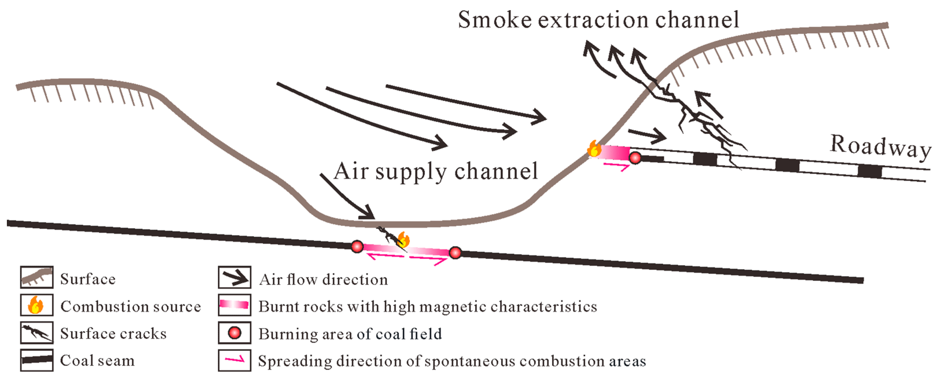
3.1. The Background of the Coalfield Spontaneous Combustion Area

The survey area is located in the western part of a coal mine in Liaoning Province, China. The spontaneous combustion phenomenon of coalfields in this area has existed for more than ten years. The side slope of the survey area has obvious smoke generated via the spontaneous combustion of subsurface coal seams (Figure 4), which has a serious impact on the surrounding ecological environment, residents’ health, and urban planning, so the spontaneous combustion area of the subsurface coal seams needs to be treated. The strata in the survey area are mainly composed of sandstone, shale, and a coal seam. The old roadway and surface crack formed through mining lead to spontaneous combustion in the survey area. The burned rock collapses and slides naturally under the action of gravity, and the sliding is aggravated under the erosion of water, which induces geological disasters such as collapses and landslides.
There is much smoke in the cracks of the side slope. Unlike the geological conditions of other places, there are a large number of roadways distributed on the side slope of the survey area, and the location of the roadway is unknown due to the long mining age. The air channel of the survey area is mainly composed of roadways and surface cracks.

3.2. The Geophysical Characteristics of the Coalfield Spontaneous Combustion Area

There are many spontaneous combustion phenomena that are affected by the coal fire combustion system in the survey area. The burned area and the burning area constitute the range of the coalfield spontaneous combustion area, and this range can be effectively identified by detecting burnt rocks [9,10]. We collected a variety of rock samples, including burnt rock produced via coalfield spontaneous combustion in the survey area, and we detected them using a portable magnetic susceptibility meter, SM-30. The average magnetic susceptibility of each rock sample is shown in Table 1.
The susceptibility is linearly related to the induced magnetization, and the stronger the magnetic susceptibility, the stronger the induced magnetization. It can be seen from Table 1 that the average magnetic susceptibility of burnt rock is much higher than that of other rock samples in the survey area. In addition, strong thermal remanence will accumulate during the cooling process of the burnt rocks [9]. Therefore, the geological conditions in this area are suitable for using the magnetic method to detect the burnt rock areas. During the spontaneous combustion of a coalfield, only the rock in the coal seam has the high-temperature condition necessary to form highly magnetic bodies. Therefore, the burnt rocks that can be detected via magnetic exploration are produced from the rocks in the coal seam.
The burnt rocks are not magnetic when the temperature exceeds the Curie temperature (573 degrees Celsius) [9]. This kind of burnt rock cannot be detected via magnetic exploration, so it is impossible to analyze these burnt rocks using the inversion of magnetic data [40]. Burnt rocks with a temperature higher than the Curie temperature have high-temperature characteristics and are distributed near the burning position in the coalfield. The burning position in the coalfield is the high-temperature area near the burnt rock. The high-temperature areas can be identified through infrared temperature measurements.
By comprehensively analyzing the range of the coalfield spontaneous combustion area and the location of the high-temperature area, the spread direction of spontaneous combustion in a coalfield can be inferred to provide more detailed and accurate information for coal mining and coalfield spontaneous combustion area management. Because the side slope soil is loose and the slope is large, ground measurement cannot be carried out. Therefore, airborne infrared remote sensing temperature measurement and airborne magnetic measurement are used to detect the range and state of the coalfield spontaneous combustion area, which provides a reference for the management of the coalfield spontaneous combustion area.

3.3. The Topographic Data

The topographic data of the survey area were obtained via an airborne millimeter-wave radar altimeter, and they are shown in Figure 5. The measurement accuracy of the millimeter-wave radar altimeter is better than 1 cm. The topographic data measurement was designed with observation points in a grid pattern. The spacing between each observation point was 20 m. Therefore, the resolution of the topographic data is 20 m, and the topographic data error is less than 1 cm. It can be seen that the survey area is the western part of an open-pit coal mine. The maximum altitude is about 215 m, and it is located on the southeast corner of the top platform, while the minimum altitude is about −158 m, and it is located at the bottom of the survey area. According to the terrain classification, the survey area is mainly divided into three parts: I. a top platform, II. a side slope, and III. the bottom. According to the observation of the surface and the previous information of the open-pit coal mine, the following information can be obtained: (1) The terrain of I is flat, and the surface has not been damaged by open-pit mining, but there is a situation of subsurface coal mine roadway mining in I area. (2) There are burning areas and smoke at the southern and western parts of II, so it can be determined that there are coalfield spontaneous combustion areas in II. However, since the slope of the southern part of II is large (the average slope is 33°) and the soil of II is loose, it is impossible to carry out ground and borehole surveys. Therefore, the range and state of the coalfield spontaneous combustion areas also need to be determined via airborne magnetic and airborne infrared remote sensing. The average slope of the northern part of II is 17°, and there are no burnt rock outcrops or smoke on the surface. (3) III was produced via open-pit mining, and this area contains burnt rock outcrops and smoke. There are many coal gangue heaps on the surface in the northwest of III, which have a high temperature, and they are shown in Figure 5.

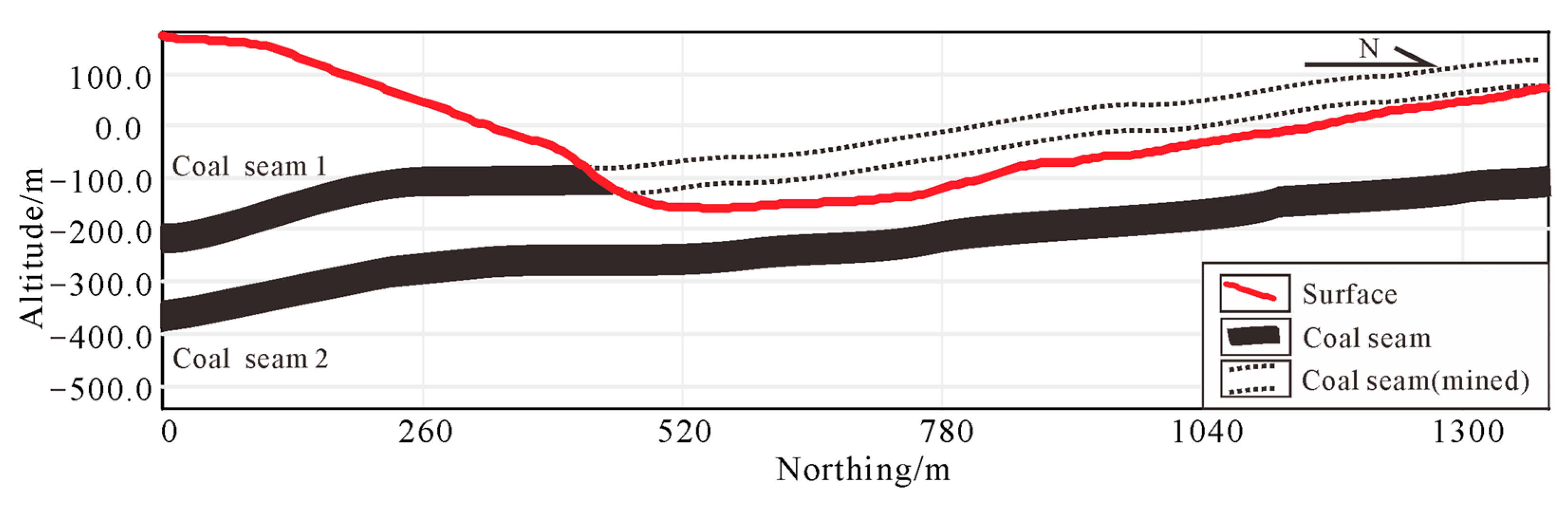
3.4. The Coal Seam Altitude Data

From the geological survey, we know that the strata in the survey area have sedimentary characteristics, and there are no large faults. Therefore, coal is distributed in layers. Through a small amount of coal outcrop, borehole, and roadway information, the altitude of the coal seam in the survey area can be obtained, and these data are also easy to obtain and practical in a coalfield. The altitude of the coal seam in the survey area is shown in Figure 6, which mainly features two coal seams. From the top to the bottom in Figure 6 are, respectively, the coal seam 1 top boundary, the coal seam 1 bottom boundary, the coal seam 2 top boundary, and the coal seam 2 bottom boundary. The open-pit mining of coal seam 1 has been carried out at the bottom and the north sides of the survey area, so coal seam 1 only exists on the south side of the survey area. Coal seam 2 is distributed throughout the survey area. The overall altitude characteristics of the coal seam are high in the northwest and low in the southeast. We extracted the north–south section with an east coordinate of 800 m to show the terrain, coal seam 1, and coal seam 2, as shown in Figure 7.
Figure 7 shows that the central and northern parts of coal seam 1 have been mined, while the southern part retains coal seam 1 with outcrops on the southern side slope, consistent with the burnt rock outcrops observed on the ground. Coal seam 2 is located under the surface, and it is closer to the surface at the bottom than other areas, which makes it more likely to undergo spontaneous combustion when in contact with air through the surface cracks.

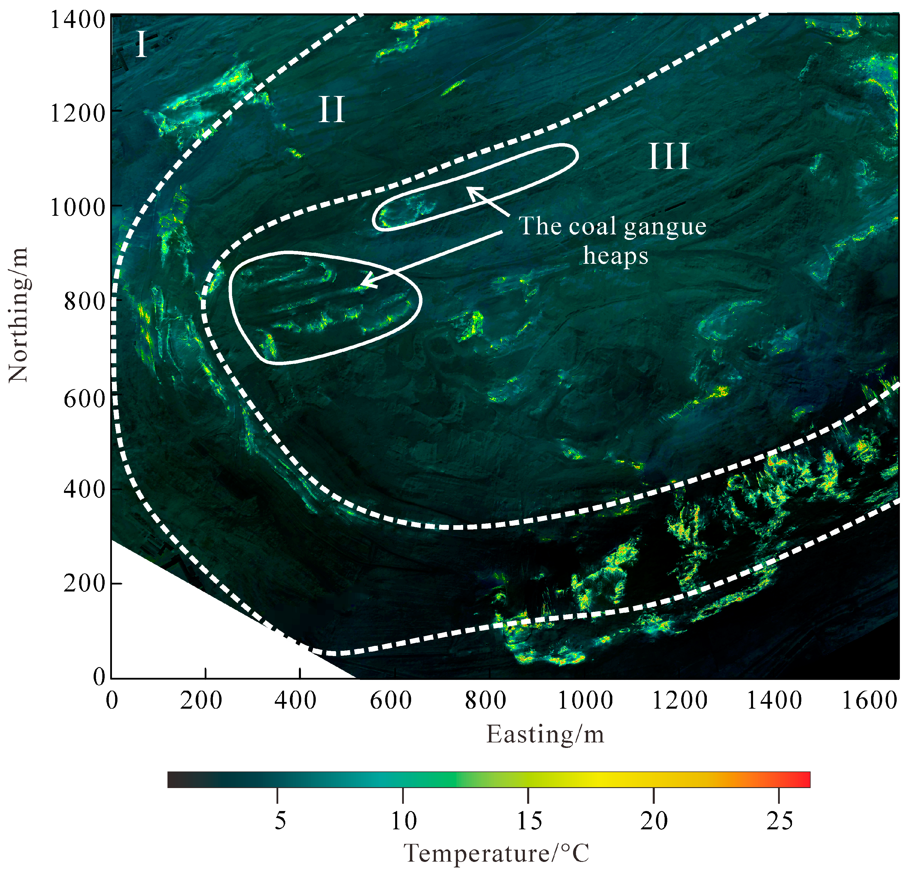
3.5. The Temperature Data of Airborne Infrared Remote Sensing Measurement

We used the FLIR VUE PRO R infrared thermal imager to measure the surface temperature of the survey area. The heading overlap of the airborne infrared measurement is 85%, and the side-lap overlap of adjacent survey lines is 65%. Finally, the temperature map with a resolution of 0.7–1.2 m was obtained as shown in Figure 8.
It can be seen from Figure 8 that the high-temperature area is mainly distributed in the southeast of Areas I–II, the northwest of Areas I–II, and some areas of Area III. The high-temperature anomalies in Area I are mainly distributed near the side slope. The part far from the side slope in Area I has compact surface soil, and it is difficult for air to circulate. The surface soil of the side slope is loose, which makes it easy for air to circulate and lead to coal spontaneous combustion. The high-temperature area on the southeast side of Area II matches the smoke of the photo in Figure 4, and it is the largest high-temperature anomaly in the survey area, indicating that this area’s coal spontaneous combustion is the most serious in the survey area. The distribution of high-temperature anomalies in Area III is relatively scattered, mainly located in the southeast, northeast, and northwest of Area III. Among them, the northwest part is the high temperature generated via the oxidation and combustion of coal gangue heaps. These high-temperature areas are regular, and they are all arc-shaped and arranged from the northwest to the southeast. This is because the coal gangue is accumulated in batches.

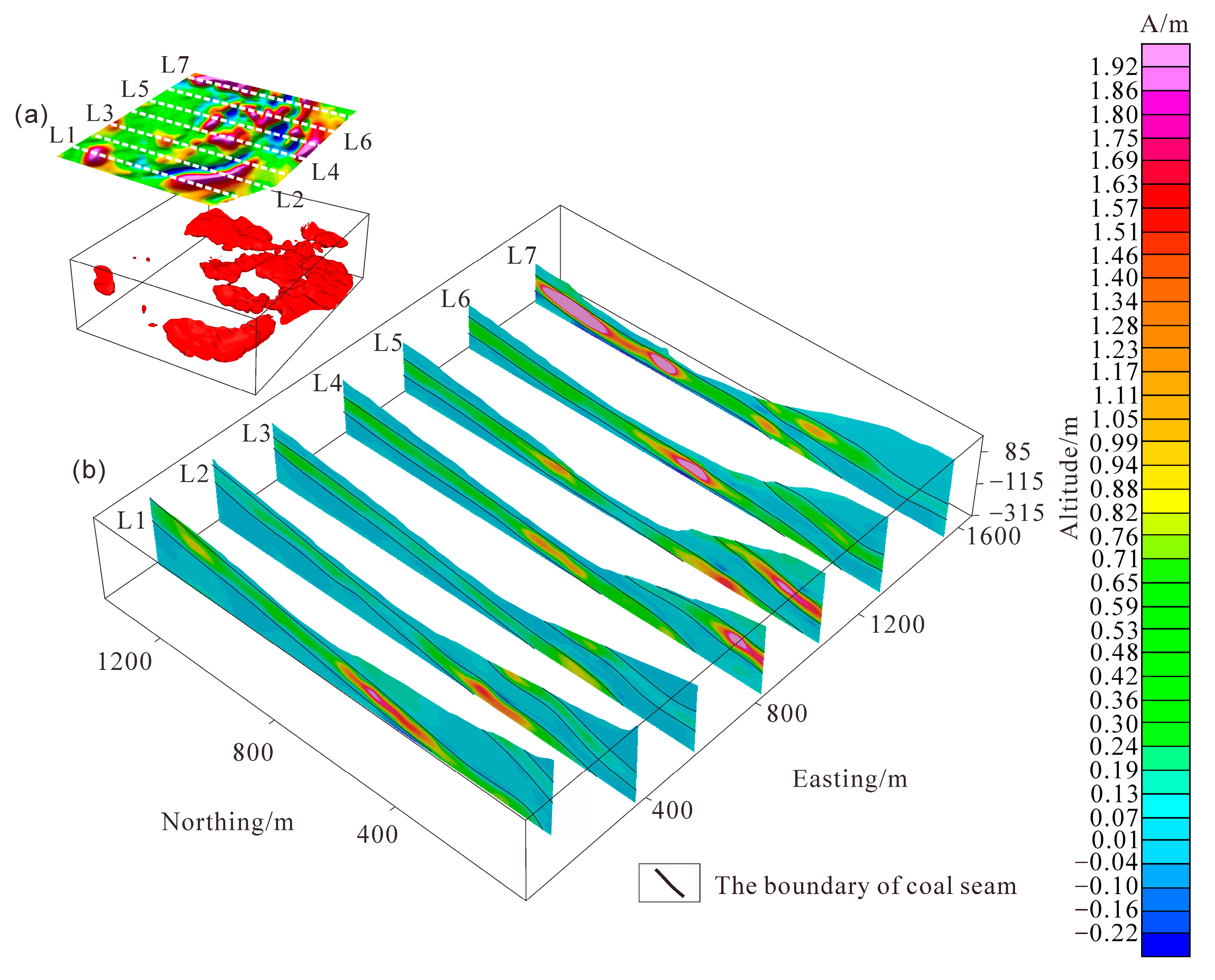
3.6. The Airborne Magnetic Data

The airborne magnetic measurement in the survey area used the DJI M300 RTK unmanned air vehicle and a rubidium optically pumped magnetometer, and the working temperature of the optically pumped magnetometer was from −20 degrees Celsius to 50 degrees Celsius; the measurement range was ±75,000 nT, the sampling frequency was 3.33 Hz, and the resolution was better than 0.3 nT. The ground magnetic station used a GSM-19T magnetometer. A UAV will have an impact on the optically pumped magnetometer, and the scope of the impact is related to factors such as the size of the UAV and the installation position of the optically pumped magnetometer [25,48]. The optically pumped magnetometer is located 1 m above the UAV, and they are connected via a non-magnetic rigid rod, as shown in Figure 9a. Moreover, during the measurement process, the yaw angle of the UAV is locked to ensure that the orientation of the probe and its relative position to the UAV do not change significantly. In this way, the magnetic measurement differences caused by different flight directions can be reduced. The measurement scale was 1:2000, and the flight height was 30 m above the ground. The direction of the survey lines was 60 degrees east of north, and the spacing between survey lines was 20 m. There were a total of 102 survey lines of varying lengths. Figure 9b shows a schematic diagram of the design of the survey lines within the survey area. In order to avoid the errors caused when a UAV flies to the next survey line, in the actual flight, both ends of each survey line were extended outward by 20 m. We selected the L1–L1’ and L2–L2’ survey lines (Figure 9b) for repeated flight along the lines to verify the measurement accuracy of the equipment, and the results are shown in Figure 9c. It can be seen that the results of the repeated measurements are basically consistent with those of the first measurement. The root mean square errors of the L1–L1’ and L2–L2’ lines are 3.4 nT and 4.2 nT, respectively.
The original data obtained were processed via bad-point elimination, correction for diurnal variation, international geomagnetic reference field correction, low-pass filtering, and other conventional processing. Figure 10 shows a magnetic map of the airborne measurement. A Butterworth filter was selected for low-pass filtering. The central wavenumber of the filter was 8.5, and the filter degree was 8. The results before and after filtering are shown in Figure 10a,b. The part that is regarded as noise and was removed is shown in Figure 10c. The data characteristics in Figure 10c have a weak correlation with the characteristics of the magnetic anomalies in Figure 10a,b, indicating that there are few target magnetic anomalies contained therein, and no obvious target information was eliminated during the low-pass filtering process. The data characteristics in Figure 10c have a strong correlation with the characteristics of the survey line layout. The strips formed by the high- and low-amplitude data have a distribution characteristic of 60 degrees east of north, which shows that they contain a lot of information obtained through the actual distribution of the survey lines. Therefore, it is in line with the characteristic of the noise being generated during the measurement process. Therefore, we believe the parameter selection for this noise removal is reasonable.
Through a comparison of Figure 10a,b, it can be seen that the low-pass filtering effectively removed the high-frequency noise and retained the main target magnetic anomaly. The strength of a magnetic anomaly is directly related to the subsurface magnetization intensity. The magnetic anomaly of non-magnetic and weakly magnetic areas was close to 0. It can be seen from Figure 10b that the strength of most anomalies was greater than 100 nT, which is consistent with the high-magnetization characteristics of a coalfield spontaneous combustion area. The main strong magnetic anomalies in Area I are on the southeast and northwest sides, and they are close to the side slope. The strong and large anomalies are mainly distributed on the southwest and southeast sides of Area II, which is consistent with the smoke locations in the photo of Figure 4. These two places include smoke extraction channels, so these areas are most fully burned and should have stronger magnetization. The strong magnetic anomalies in Area III are mainly distributed in the southeast, and the anomalies are scattered. There are only a few small magnetic anomalies at the coal gangue heaps, which are circled in Figure 10b, and the strength of magnetic anomalies is less than 10 nT. This is a weak anomaly caused by the burnt rocks in coal gangue heaps. Compared with the burnt rocks near the subsurface coalfield spontaneous combustion area, the coal gangue contains less ferromagnetic materials, and the distribution is not concentrated. Therefore, even if the accumulated surface makes the combustion more sufficient, there is no obvious anomaly. Whether the spontaneous combustion areas represented by the above strong magnetic anomalies are connected to each other and the ranges of spontaneous combustion areas needs to be analyzed according to the inversion results.

4. Results

Using topographic data, we divided the subsurface from the surface to the altitude of −315 m in the horizontal range of the topographic data into 16,167 closely tetrahedral cells, and we calculated the responses of the cells at the observation points to form a kernel matrix for inversion. According to the coal seam information (the altitudes of the top and bottom interfaces of the coal seam), we set the magnetization intensity of the prior model to 0 and use D to extract the solution parameters of the subdivision cells outside the coal seam. We obtained subsurface magnetization through the a priori information-constrained inversion of the magnetic data, and we obtained isosurface and slice mapping of three-dimensional magnetization in the survey area, as shown in Figure 11.
We set the magnetization value of the isosurface based on the condition that the isosurface matches the maximum gradient region between the high and low magnetizations in the inversion results. Figure 11a depicts the magnetic anomaly and the isosurface with 0.31 A/m. It also indicates the inferred three-dimensional boundary of the coalfield spontaneous combustion area. It can be seen that the distribution of high-magnetization bodies matches the distribution of strong magnetic anomalies.
Figure 11b shows that there are no high-magnetization anomalies out of a coal seam, indicating that the constrained inversion of magnetic data based on the a priori model can effectively control the magnetization anomalies’ area so that the inversion results are more in line with the actual situation. Finally, combining the three-dimensional range-top view of the inferred coalfield spontaneous combustion areas with the high-temperature anomaly positions in the infrared temperature measurement results, the comprehensive interpretation map of the coalfield spontaneous combustion areas is shown in Figure 12.

5. Discussion

It can be seen from Figure 12 that the high-temperature anomalies are concentrated around the spontaneous combustion areas inferred via magnetic inversion except for the coal gangue heaps. Some high-temperature anomalies are only near the periphery of the inferred spontaneous combustion areas, which is because the coalfield spontaneous combustion temperature is higher than the Curie temperature, resulting in the rocks near it becoming non-magnetic. This kind of high-temperature anomaly reveals new spontaneous combustion areas of the coalfield. Some high-temperature anomalies are located in the range of the inferred coalfield spontaneous combustion areas. It may be that coal combustion does not heat the nearby rocks above the Curie temperature, and most of them are the older coalfield combustion areas that will be burned out. Some inferred spontaneous combustion areas have no high-temperature anomalies, indicating that the spontaneous combustion areas in this range have been extinguished due to coal burnout, and they are the oldest spontaneous combustion areas of the survey area.
Through the analysis of the new and old coalfield spontaneous combustion areas, it can be inferred that the future spread direction of the coalfield spontaneous combustion areas is from the old areas to the new areas, which is indicated by the arrow in Figure 12. Four boreholes were created to verify the ranges of the inferred coalfield spontaneous combustion areas. It was found that the inferred results are accurate, and the depth of the inferred spontaneous combustion area is consistent with the depth of the burnt rock in the borehole. In Figure 12, black and green signs are used to mark the location of a borehole and whether there are burnt rocks. The final inference results can be divided into nine blocks from “a” to “i” for discussion. The inversion results of each block imply the depth of the spontaneous combustion areas, as shown in Table 2.
The following inferences were obtained by analyzing each block in Figure 12:
(1)
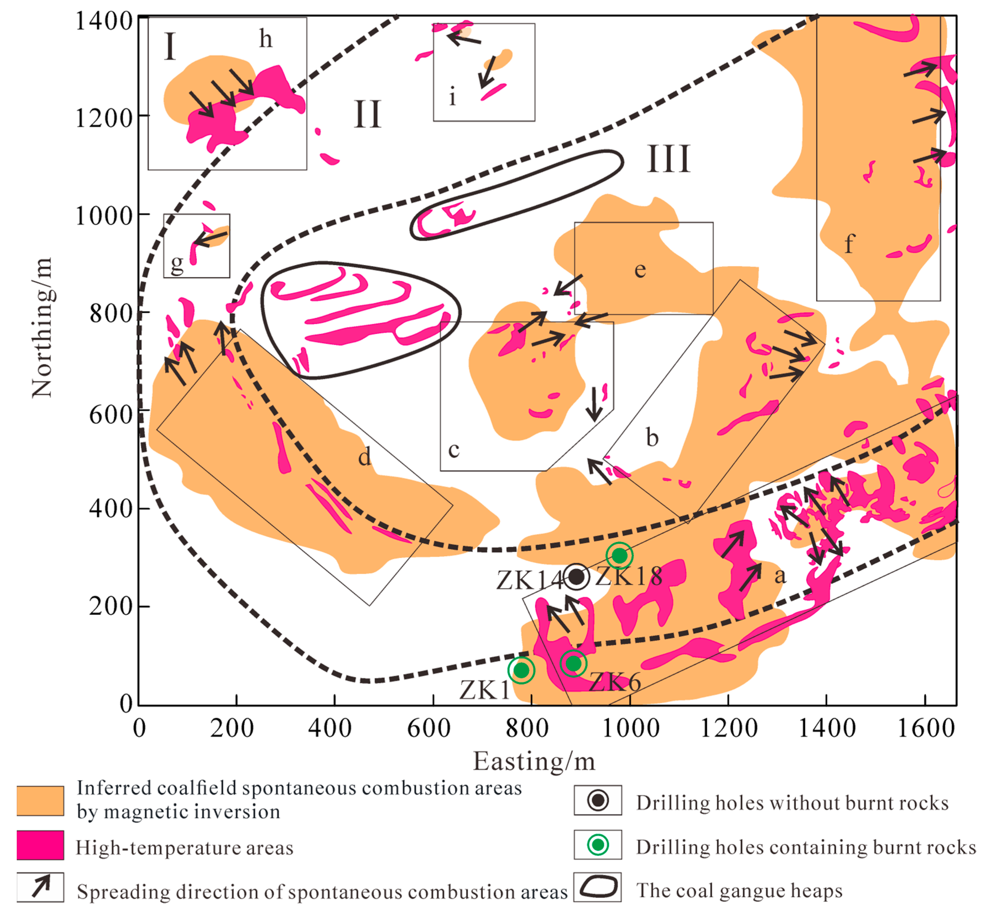
“Block a” has the largest areas of high-temperature anomalies, and there is smoke on the surface, so it is the most serious area of spontaneous combustion. However, most of the high-temperature anomalies are located in the inferred coalfield spontaneous combustion areas, indicating that these high-temperature anomalies correspond to the old spontaneous combustion areas. Therefore, it is speculated that the coals around these high-temperature anomalies are basically burned out, and the temperature will gradually decrease. In contrast, the spontaneous combustion areas in the middle of “Block a” will spread to the northeast, southeast, and northwest sides, as shown in Figure 12, while those at the northwest corner will spread northwest, as shown in Figure 12.
(2)
“Block b” is connected to “Block a” and “Block e”, and the high-temperature anomalies are mostly within the inferred coalfield spontaneous combustion areas. The coal seam near these high-temperature anomalies is also inferred to lead to a subsequent temperature decrease. As shown in Figure 12, it is inferred that the spontaneous combustion areas at the eastern corner of “Block b” will spread eastward, while those at the western corner will spread northwestward and connect with “Block c” in the future.
(3)
“Block c” is connected to “Block e”, and from the high-temperature anomalies outside the inferred coalfield spontaneous combustion areas at the northeast and southeast sides of “Block c”, it is inferred that the coalfield spontaneous combustion areas will spread in the direction shown in Figure 12 in the future and will be connected with “Block b”.
(4)
“Block d” is not connected to other blocks at present, and the high-temperature anomalies are mostly within the inferred coalfield spontaneous combustion areas. The coal seam near these high-temperature anomalies is also inferred to undergo a subsequent temperature decrease. On the northwest side of “Block d”, there are some high-temperature anomalies outside the inferred coalfield spontaneous combustion areas. Therefore, it is deduced that these inferred coalfield spontaneous combustion areas will spread northwestward, as shown in Figure 12, and gradually connect with “Block g”.
(5)
“Block e” is connected to “Block b” and “Block c”, and there are no high-temperature anomalies in the inferred coalfield spontaneous combustion areas, and it is inferred that the coalfield spontaneous combustion areas in this block are older than those in other blocks. At present, the coal seam is in a state in which the temperature has decreased after spontaneous combustion. On the southwest side of “Block e”, there are some high-temperature anomalies outside the inferred coalfield spontaneous combustion areas. Therefore, it is inferred that coalfield spontaneous combustion areas will spread southwestward, as shown in Figure 12.
(6)
“Block f” is connected to “Block a” and “Block b”, and the high-temperature anomalies are located at the east of inferred coalfield spontaneous combustion areas. Therefore, it is deduced that these inferred coalfield spontaneous combustion areas will spread eastward, as shown in Figure 12, and ignite the coal to the east side of the survey area.
(7)
“Block g” is not connected to other blocks at present, and it has the smallest inferred coalfield spontaneous combustion areas. Therefore, it is deduced that these inferred coalfield spontaneous combustion areas are newer than those in other blocks. The spread state of these inferred coalfield spontaneous combustion areas is not stable. Based on the current data, it is speculated that the inferred coalfield spontaneous combustion areas will spread westward in the future, but this inference has great instability.
(8)
“Block h” is not connected to other blocks at present, and the high-temperature anomalies are located at the southeast of inferred coalfield spontaneous combustion areas. Therefore, it is deduced that these inferred coalfield spontaneous combustion areas will spread southeastward, as shown in Figure 12.
(9)
“Block i” is similar to “Block g”, and the inferred coalfield spontaneous combustion areas are small. Based on the current data, it is speculated that the inferred coalfield spontaneous combustion areas will spread westward and southwestward, but this inference has great instability.

6. Conclusions

For the high-precision exploration of coalfield spontaneous combustion areas via magnetic and infrared remote sensing data, we have proposed a constrained magnetization vector inversion method based on coal seam information, and we have combined the infrared temperature data with the inversion results to infer the ranges, states, and spread directions of coalfield spontaneous combustion areas in Liaoning Province, China. Verified via artificial model tests, the constrained inversion of magnetic data based on coal seam information can obtain more accurate inversion results and improve the matching degree between the inversion results and the actual situation. Combining the constrained inversion results of magnetic data with the high-temperature areas of infrared remote sensing data can help us infer the range, state, and future spread direction of coalfield spontaneous combustion areas. The main coalfield spontaneous combustion areas in the survey area of Liaoning Province, China, were divided into nine blocks, some of which are connected. Among them, “Block a” is the most serious spontaneous combustion area, “Block e” is an older spontaneous combustion area than the others, and “Block i” and “Block g” are newer spontaneous combustion areas than the others; through the location of high-temperature anomalies and inferred coalfield spontaneous combustion areas, it was reasoned that the future of the coalfield spontaneous combustion areas will produce more connectivity.

Author Contributions

Conceptualization, G.M.; methodology, Q.M.; software, L.L.; formal analysis, J.L.; data curation, J.L.; writing—original draft preparation, Q.M.; writing—review and editing, L.L. and J.L.; visualization, Q.M.; supervision, G.M.; project administration, Q.M. All authors have contributed significantly and participated sufficiently to take responsibility for this research. All authors have read and agreed to the published version of the manuscript.

Funding

This research was funded by the National Natural Science Foundation of China (grant number: 42304150).

Data Availability Statement

The original contributions presented in this study are included in the article. Further inquiries can be directed to the corresponding author.

Conflicts of Interest

The authors declare that they have no conflicts of interest.

References

  1. Glenn, B.; Tammy, P. Coal fires burning out of control around the world: Thermodynamic recipe for environmental catastrophe. Int. J. Coal Geol. 2004, 59, 7–17. [Google Scholar] [CrossRef]
  2. Cao, Q.; Yan, S.; Xue, G.; Zhu, N. High resolution resistivity detecting and remote internet monitoring of coalfield fire. Chin. J. Geophys. 2017, 60, 424–429. (In Chinese) [Google Scholar] [CrossRef]
  3. Zheng, Y.; Li, Q.; Zhu, P.; Li, X.; Zhang, G.; Ma, X.; Zhao, Y. Study on Multi-field Evolution and Influencing Factors of Coal Spontaneous Combustion in Goaf. Combust. Sci. Technol. 2021, 195, 247–264. [Google Scholar] [CrossRef]
  4. Ma, Z.; Qin, B.; Shi, Q.; Zhu, T.; Chen, X.; Liu, H. The location analysis and efficient control of hidden coal spontaneous combustion disaster in coal mine goaf: A case study. Process Saf. Environ. Prot. 2024, 184, 66–78. [Google Scholar] [CrossRef]
  5. Chen, J.; Li, L.; Jiang, D.; Zhou, L.; Wang, L. Experimental study on the spatial and temporal variations of temperature and indicator gases during coal spontaneous combustion. Energy Explor. Exploit. 2021, 39, 354–366. [Google Scholar] [CrossRef]
  6. Gao, S.; Gao, D.; Liu, Y.; Chai, J.; Chen, J. Distribution Law of Coal Spontaneous Combustion Hazard Area in Composite Goaf of Shallow Buried Close Distance Coal Seam Group. Combust. Sci. Technol. 2021, 195, 1960–1980. [Google Scholar] [CrossRef]
  7. Shi, X. Research and application of comprehensive electromagnetic detection technique in spontaneous combustion area of coalfields. Saf. Sci. 2012, 50, 655–659. [Google Scholar] [CrossRef]
  8. Anghelescu, L.; Diaconu, B.M. Advances in Detection and Monitoring of Coal Spontaneous Combustion: Techniques, Challenges, and Future Directions. Fire 2024, 7, 354. [Google Scholar] [CrossRef]
  9. Shao, Z.; Wang, D.; Wang, Y.; Zhong, X. Theory and application of magnetic and self-potential methods in the detection of the Heshituoluogai coal fire, China. J. Appl. Geophys. 2014, 104, 64–74. [Google Scholar] [CrossRef]
  10. Zhang, B.; Xiao, F.; Jin, W. Burnt coal field detection via magnetic exploration. Environ. Earth Sci. 2023, 82, 160. [Google Scholar] [CrossRef]
  11. Ma, G.; Ma, S.; Li, L.; Cai, J. Method of self-structure-constrained inversion of magnetic anomalies and their magnetic gradients and its application in the exploration of coal burning area. Prog. Geophys. 2024, 39, 1026–1037. (In Chinese) [Google Scholar] [CrossRef]
  12. Ide, T.S.; Crook, N.; Orr, F.M., Jr. Magnetometer measurements to characterize a subsurface coal fire. Int. J. Coal Geol. 2011, 87, 190–196. [Google Scholar] [CrossRef]
  13. Liang, S.; Sun, S.; Lu, H. Application of Airborne Electromagnetics and Magnetics for Mineral Exploration in the Baishiquan–Hongliujing Area, Northwest China. Remote Sens. 2021, 13, 903. [Google Scholar] [CrossRef]
  14. Accomando, F.; Bonfante, A.; Buonanno, M.; Natale, J.; Vitale, S.; Florio, G. The drone-borne magnetic survey as the optimal strategy for high-resolution investigations in presence of extremely rough terrains: The case study of the Taverna San Felice quarry dike. J. Appl. Geophys. 2023, 217, 105186. [Google Scholar]
  15. Ma, G.; Meng, L.; Li, L. Fast Magnetization Vector Inversion Method with Undulating Observation Surface in Spherical Coordinate for Revealing Lunar Weak Magnetic Anomaly Feature. Remote Sens. 2024, 16, 432. [Google Scholar] [CrossRef]
  16. Shi, X.; Geng, H.; Liu, S. Magnetization Vector Inversion Based on Amplitude and Gradient Constraints. Remote Sens. 2022, 14, 5497. [Google Scholar] [CrossRef]
  17. Ma, G.; Zhao, Y.; Xu, B.; Li, L.; Wang, T. High-Precision Joint Magnetization Vector Inversion Method of Airborne Magnetic and Gradient Data with Structure and Data Double Constraints. Remote Sens. 2022, 14, 2508. [Google Scholar] [CrossRef]
  18. Kim, B.; Jeong, S.; Bang, E.; Shin, S.; Cho, S. Investigation of Iron Ore Mineral Distribution Using Aero-Magnetic Exploration Techniques: Case Study at Pocheon, Korea. Minerals 2021, 11, 665. [Google Scholar] [CrossRef]
  19. Liu, S.; Tan, H.; Peng, M.; Li, Y. Three-Dimensional Limited-Memory BFGS Inversion of Magnetic Data Based on a Multiplicative Objective Function. Appl. Sci. 2023, 13, 11198. [Google Scholar] [CrossRef]
  20. Meng, Q.; Ma, G.; Li, L.; Wang, T.; Li, Z.; Wang, N. Joint Inversion of Gravity and Magnetic Data with Tetrahedral Unstructured Grid and its Application to Mineral Exploration. IEEE Trans. Geosci. Remote Sens. 2023, 61, 5915514. [Google Scholar] [CrossRef]
  21. Abbas, M.A.; Speranza, L.; Fedi, M.; Garcea, B.; Bianco, L. Magnetic data modelling of salt domes in Eastern Mediterranean, offshore Egypt. Acta Geophys. 2024, 72, 1293–1303. [Google Scholar]
  22. Wang, C.; Hu, P.; Sun, Y.; Yang, C. Study on CO source identification and spontaneous combustion warning concentration in the return corner of working face in shallow buried coal seam. Environ. Sci. Pollut. Res. 2024, 31, 15050–15064. [Google Scholar] [CrossRef]
  23. Zhou, L.; Zhang, D.; Wang, J.; Huang, Z.; Pan, D. Mapping Land Subsidence Related to Underground Coal Fires in the Wuda Coalfield (Northern China) Using a Small Stack of ALOS PALSAR Differential Interferograms. Remote Sens. 2013, 5, 1152–1176. [Google Scholar] [CrossRef]
  24. Stoll, J.; Moritz, D. Unmanned aircraft systems for rapid near surface geophysical measurements. In Proceedings of the 75th EAGE Conference & Exhibition-Workshops, London, UK, 10–13 June 2013. [Google Scholar]
  25. Accomando, F.; Vitale, A.; Bonfante, A.; Buonanno, M.; Florio, G. Performance of two different flight configurations for drone-borne magnetic data. Sensors 2021, 21, 5736. [Google Scholar] [CrossRef]
  26. Dual Mag System. Available online: http://www.mgt-geo.com/dual%20mag%20system.htm (accessed on 22 July 2021).
  27. Mu, Y.; Zhang, X.; Xie, W.; Zheng, Y. Automatic detection of near-surface targets for unmanned aerial vehicle (UAV) magnetic survey. Remote Sens. 2020, 12, 452. [Google Scholar] [CrossRef]
  28. Parvar, K.; Braun, A.; Layton-Matthews, D.; Burns, M. UAV magnetometry for chromite exploration in the Samail ophiolite sequence, Oman. J. Unmanned Veh. Syst. 2017, 6, 57–69. [Google Scholar]
  29. Malehmir, A.; Dynesius, L.; Paulusson, K.; Paulusson, A.; Johansson, H.; Bastani, M.; Wedmark, M.; Marsden, P. The potential of rotary-wing UAV-based magnetic surveys for mineral exploration: A case study from central Sweden. Lead. Edge 2017, 36, 552–557. [Google Scholar]
  30. Cunningham, M.; Samson, C.; Wood, A.; Cook, I. Aeromagnetic surveying with a rotary-wing unmanned aircraft system: A case study from a zinc deposit in Nash Creek, New Brunswick, Canada. Pure Appl. Geophys. 2018, 175, 3145–3158. [Google Scholar]
  31. Walter, C.; Braun, A.; Fotopoulos, G. High-resolution unmanned aerial vehicle aeromagnetic surveys for mineral exploration targets. Geophys. Prospect. 2020, 68, 334–349. [Google Scholar]
  32. Schmidt, V.; Becken, M.; Schmalzl, J. A UAV-borne magnetic survey for archaeological prospection of a Celtic burial site. First Break 2020, 38, 61–66. [Google Scholar]
  33. Accomando, F.; Florio, G. Drone-Borne Magnetic Gradiometry in Archaeological Applications. Sensors 2024, 24, 4270. [Google Scholar] [CrossRef] [PubMed]
  34. Yu, B.; She, J.; Liu, G.; Ma, D.; Zhang, R.; Zhou, Z.; Zhang, B. Coal fire identification and state assessment by integrating multitemporal thermal infrared and InSAR remote sensing data: A case study of Midong District, Urumqi, China. ISPRS J. Photogramm. Remote Sens. 2022, 190, 144–164. [Google Scholar] [CrossRef]
  35. Pandey, J.; Kumar, D.; Mishra, R.K.; Mohalik, N.K.; Khalkhoand, A.V.K. Application of Thermography Technique for Assessment and Monitoring of Coal Mine Fire: A Special Reference to Jharia Coal Field, Jharkhand, India. Singh Int. J. Adv. Remote Sens. GIS 2013, 2, 138–147. [Google Scholar]
  36. Wang, H.; Fang, X.; Li, Y.; Zheng, Z.; Shen, J. Research and application of the underground fire detection technology based on multi-dimensional data fusion. Tunn. Undergr. Space Technol. 2021, 109, 103753. [Google Scholar] [CrossRef]
  37. Wang, H.; Fan, C.; Chen, L.; Chen, X.; Zhang, J.; Zhong, H. Research on early identification of burning status in a fire area in Xinjiang based on data-driven. Case Stud. Therm. Eng. 2024, 60, 104685. [Google Scholar] [CrossRef]
  38. Chiu, L.S.-Y.; Lai, W.W.-L.; Santos-Assunção, S.; Sandhu, S.S.; Sham, J.F.-C.; Chan, N.F.-S.; Wong, J.C.-F.; Leung, W.-K. A Feasibility Study of Thermal Infrared Imaging for Monitoring Natural Terrain—A Case Study in Hong Kong. Remote Sens. 2023, 15, 5787. [Google Scholar] [CrossRef]
  39. Frodella, W.; Elashvili, M.; Spizzichino, D.; Gigli, G.; Adikashvili, L.; Vacheishvili, N.; Kirkitadze, G.; Nadaraia, A.; Margottini, C.; Casagli, N. Combining InfraRed Thermography and UAV Digital Photogrammetry for the Protection and Conservation of Rupestrian Cultural Heritage Sites in Georgia: A Methodological Application. Remote Sens. 2020, 12, 892. [Google Scholar] [CrossRef]
  40. Li, Y.; Oldenburg, D. 3-D inversion of magnetic data. Geophysics 1996, 61, 394–408. [Google Scholar]
  41. Meng, Q.; Ma, G.; Li, L.; Wang, T.; Li, Z.; Li, J. The ES-GNF Method of Unstructured Tetrahedral Mesh for Fast Inversion of Gravity and Magnetic Data with Undulating Terrain. IEEE Trans. Geosci. Remote Sens. 2024, 62, 5934215. [Google Scholar] [CrossRef]
  42. Ghalehnoee, M.H.; Ansari, A. Compact magnetization vector inversion. Geophys. J. Int. 2021, 228, 1–16. [Google Scholar]
  43. Meng, Q.; Ma, G.; Li, L.; Wang, T.; Han, J. 3-D cross-gradient joint inversion method for gravity and magnetic data with unstructured grids based on second-order taylor formula: Its application to the southern Greater Khingan range. IEEE Transac. Geosci. Remote Sens. 2022, 60, 5914816. [Google Scholar]
  44. Bianco, L.; Tavakoli, M.; Vitale, A.; Fedi, M. Multiorder sequential joint inversion of gravity data with inhomogeneous depth weighting: From near surface to basin modeling applications. IEEE Trans. Geosci. Remote Sens. 2023, 62, 4700311. [Google Scholar]
  45. Vitale, A.; Fedi, M. Self-constrained inversion of potential fields through a 3D depth weighting. Geophysics 2020, 85, G143–G156. [Google Scholar]
  46. Hansen, P.C. Analysis of discrete ill-posed problems by means of the L-curve. SIAM Rev. 1992, 34, 561–580. [Google Scholar]
  47. Shewchuk, J.R. Delaunay refinement algorithms for triangular mesh generation. Comput. Geom. 2002, 22, 21–74. [Google Scholar] [CrossRef]
  48. Walter, C.; Braun, A.; Fotopoulos, G. Characterizing electromagnetic interference signals for unmanned aerial vehicle geophysical surveys. Geophysics 2021, 86, J21–J32. [Google Scholar] [CrossRef]
Figure 1. The formation and characteristics of coalfield spontaneous combustion.
Remotesensing 17 01185 g001
Figure 2. Comparison of inversion results of artificial models; (a) is the three-dimensional distribution of the models and their magnetic anomaly, (b) is the slice (y = 1000 m) of the subsurface magnetization result from inversion without constraint, and (c) is the slice (y = 1000 m) of the a priori information-constrained inversion result. The white boxes indicate the positions and ranges of the models in the slices.
Remotesensing 17 01185 g002
Figure 3. Comparison of inversion results of artificial models with noise; (a) is the three-dimensional distribution of the models and their magnetic anomaly with the noise of a signal-to-noise ratio of 30, (b) is the slice (y = 1000 m) of the subsurface magnetization result from the inversion without constraint, and (c) is the slice (y = 1000 m) of the a priori information-constrained inversion result. The white boxes indicate the positions and ranges of the models in the slices.
Remotesensing 17 01185 g003
Figure 4. Photos of the topography and smoke in the survey area.
Remotesensing 17 01185 g004
Figure 5. Topographic map of the survey area.
Remotesensing 17 01185 g005
Figure 6. Altitude map of coal seams in the survey area.
Remotesensing 17 01185 g006
Figure 7. Profile of a coal seam in the survey area.
Remotesensing 17 01185 g007
Figure 8. Temperature map of airborne infrared remote sensing measurement.
Remotesensing 17 01185 g008
Figure 9. Schematic diagram of the UAV airborne magnetic survey design; (a) is the UAV airborne magnetic survey equipment, (b) is the schematic diagram of the designed survey lines, and (c) is the magnetic data obtained from repeated measurements.
Remotesensing 17 01185 g009
Figure 10. Magnetic map of airborne measurements; (a) is a gridded map of the magnetic anomaly data before the process of low-pass filtering, (b) is a gridded map of the magnetic anomaly data after the process of low-pass filtering, and (c) is the difference in magnetic anomalies before and after the process of low-pass filtering.
Remotesensing 17 01185 g010
Figure 11. The isosurface and slice mapping of magnetic inversion results; (a) shows the isosurface with M = 0.31 A/m, and (b) shows the slice mapping from Line 1 to Line 7 (L1 to L7).
Remotesensing 17 01185 g011
Figure 12. Comprehensive interpretation map of the coalfield spontaneous combustion areas.
Remotesensing 17 01185 g012
Table 1. The average magnetic susceptibility of rock samples.
The Rock Sample TypeThe Average Magnetic Susceptibility (SI)
1Mudstone0.42 × 10−3
2Sandstone0.41 × 10−3
3Conglomerate0.13 × 10−3
4Coal0.02 × 10−3
5Burnt rock2.71 × 10−3
Table 2. Depth of inferred coalfield spontaneous combustion areas.
AreasThe Center Altitude of Coalfield Spontaneous Combustion Areas (m)
Block a−79.57
Block b−246.92
Block c−224.23
Block d−241.25
Block e−201.54
Block f−187.36
Block g−107.93
Block h36.73
Block i−99.43
Disclaimer/Publisher’s Note: The statements, opinions and data contained in all publications are solely those of the individual author(s) and contributor(s) and not of MDPI and/or the editor(s). MDPI and/or the editor(s) disclaim responsibility for any injury to people or property resulting from any ideas, methods, instructions or products referred to in the content.

