Abstract
Gravity inversion plays a crucial role in mineral exploration and resource evaluation, yet conventional depth-weighting methods often impose uniform resolution across all depths and fail to effectively delineate anomaly boundaries. This study presents an innovative attentional depth-weighting matrix based on a regularized downward continuation (RDC) mechanism. First, the observed gravity data are projected to greater depths using RDC, which suppresses high-frequency noise amplification. Next, gradient extrema are extracted from each grid cell to identify anomaly boundaries, forming a constant weighting matrix that enhances the focus on target regions. This matrix is then integrated with traditional depth weighting and a minimum-support focusing factor to optimize the inversion process. The proposed method is validated through two synthetic models, demonstrating improved resolution of deeper targets and more accurate amplitude recovery compared to conventional approaches. Further application to the Dahongshan Copper–Iron Ore region in Yunnan, China, reveals a deep intrusive body at approximately 4–5 km depth, extending east–west with a distinct “U”-shaped geometry. These results, consistent with previous geological studies, highlight the method’s ability to enhance deep anomaly characterization while effectively suppressing shallow noise interference. By balancing noise reduction with improved resolution, this approach broadens the applicability of gravity inversion in geological, geothermal, and mineral resource exploration.
1. Introduction
Gravity inversion is a critical tool for delineating subsurface geological structures by interpreting density variations from observed gravity anomalies. It effectively identifies ore bodies, fault zones, and other structural features, thereby providing essential geophysical constraints for mineral exploration, resource evaluation, and environmental studies. Consequently, accurate gravity inversion underpins geological interpretation, reduces drilling costs, and enhances exploration efficiency. Moreover, by revealing density variations at greater depths, it enriches our understanding of the Earth’s internal processes and informs further investigations into geodynamic mechanisms and tectonic evolution [1,2,3,4,5,6,7,8].
Downward continuation (DC) is commonly applied to extend potential-field data measured at the surface into deeper subsurface regions, effectively enhancing anomaly signals from deeper geological bodies [9]. Upward continuation typically highlights broader, large-scale anomalies by suppressing shallow, short-wavelength signals. However, downward continuation inherently amplifies high-frequency noise, leading to computational instability and unreliable inversion results. To mitigate this ill-posed nature, regularization techniques are commonly incorporated, constraining the solution to suppress noise amplification and improve numerical stability. In this study, DC was specifically adopted rather than upward continuation, given our primary objective of accurately resolving anomaly boundaries and internal structures at depth, thus facilitating a detailed and precise delineation of subsurface geological features [9,10,11,12,13,14,15,16]. However, DC inherently amplifies high-frequency noise, thereby increasing the sensitivity of the results to measurement errors and potentially compromising their fidelity in representing true geological structures. Additionally, the gravity field obtained at a specified depth provides only an indication of general anomaly trends rather than a direct or detailed image of subsurface structures. Consequently, DC results alone are not suitable for precise structural imaging without further integration into regularized inversion frameworks.
Copper–iron ore bodies typically exhibit higher densities, thereby generating pronounced Bouguer gravity anomalies relative to surrounding host rocks [17,18,19,20,21]. Gravity inversion leverages these anomalies to delineate subsurface density distributions, essential for accurately locating ore bodies and structural boundaries. However, existing gravity inversion methods encounter notable limitations, particularly in the accurate resolution of deep subsurface targets. Due to the natural attenuation of gravity signals with increasing depth, deeper structures often exhibit reduced inversion resolution, weakening the reliability of deep geological interpretations. Additionally, traditional inversion approaches frequently produce blurred or indistinct anomaly boundaries, especially in regions characterized by complex geological settings, making it difficult to clearly delineate structural details. Consequently, these methods struggle to precisely represent the geometry and interfaces of subsurface anomalies, particularly in structurally intricate environments.
In gravity inversion, ensuring the physical realism and geological interpretability of the inverted models is crucial. One effective strategy to achieve this involves applying depth-weighting approaches that penalize deviations from prior model parameters. Such approaches compensate for the natural decline in inversion sensitivity with increasing depth, thus enhancing the resolution and stability of deep structural features and improving inversion accuracy [22,23,24,25,26]. Building on this principle, Li and Oldenburg [27,28] proposed a depth-weighting scheme that assigns distinct weights to each layer within the inversion domain, thereby moderating the sensitivity attenuation typically encountered at depth. By adjusting the weighting parameters according to the specific depth of geological targets, this method offers substantial flexibility, significantly improving inversion outcomes across various geological settings [29,30,31,32,33,34]. Nevertheless, the process of determining optimal weighting parameters often requires iterative trials and manual adjustments, introducing subjectivity and potential uncertainties into the inversion results. Subsequently, Zhdanov [35] introduced an adaptive depth-weighting method derived from the sensitivity matrix, designed to maintain consistent resolution across different model parameters, thereby effectively reducing parameter uncertainties and inversion instabilities [36,37,38]. Nevertheless, conventional gravity inversion methods typically employ a uniform depth-weighting strategy, neglecting the fact that geological structures contribute unevenly to the observed gravity anomalies at different depths. This uniform approach has inherent limitations, especially in accurately recovering deeper geological targets. Specifically, such uniform weighting often fails to adequately capture detailed structural features at greater depths, resulting in blurred or indistinct boundaries of deeper anomalies. Consequently, the fidelity of deep structure delineation is compromised. To address these limitations, it is essential to adopt depth-weighting schemes that better represent the variable contributions of geological structures at different depths. This refinement is crucial for enhancing the accuracy, resolution, and interpretive reliability of gravity inversion results, particularly in complex geological environments.
Accurately defining the top and bottom boundaries of an anomaly is critical for inversion quality, as these constraints determine the effective depth range and structural stability of the recovered geological model. Improperly set upper boundaries may lead to underestimation of shallow anomaly densities and loss of near-surface structural details, while inaccuracies in lower boundary constraints can introduce artificial deep anomalies, distorting the true subsurface structure. Commer [39] attempted to address this issue by incorporating top and bottom boundary constraints into depth weighting and integrating it with Zhdanov’s [35] minimum-support focusing inversion. While this approach improved targeting of specific anomalous layers [40,41], it primarily relied on central depth rather than fully exploiting upper and lower boundary constraints, limiting its ability to accurately capture differential contributions to the gravity field.
In this study, we present a novel attentional depth-weighting approach grounded in the regularized downward continuation (RDC) mechanism within a Tikhonov regularization framework. First, RDC is applied to extrapolate surface gravity data downward, effectively mitigating the high-frequency noise typically encountered in standard downward continuation. Next, gradient extrema are calculated in each grid cell of the downward-continued data to precisely delineate the top and bottom boundaries of subsurface anomalies. These well-defined boundaries form the basis for constructing our attentional depth-weighting matrix, which focuses the inversion on critical regions. The resulting matrix is then integrated with a traditional depth-weighting matrix and a minimum-support focusing factor, culminating in an enhanced, attentional inversion strategy. To objectively assess this method’s ability to recover deeper geological structures and their amplitudes, two synthetic models were devised and analyzed. The algorithm was subsequently applied to real gravity data from the Dahongshan Copper–Iron Ore region in Yunnan, China, aiming to characterize deep intrusive bodies that extend in an east–west direction.
2. Materials and Methods
2.1. Regularized Downward Continuation (RDC)
Consider a subsurface domain divided into regular cubic cells, with observation points located on the ground surface. The relationship between the observed data, , and the subsurface physical property (e.g., density) parameters, , is given by
where the matrix is a forward modeling operator that represents the linear relationship between the density distribution and the observed gravity anomaly , where can also be represented by , denoting the measured data at the ground surface . Let be the field value at an arbitrary point in the subsurface. Because gravitational and other potential fields in free space satisfy Laplace’s equation , DC can be performed via frequency-domain operations on . Specifically, we begin by applying the Fourier transform to , as expressed in Equation (2) as follows:
where the parameters and represent the frequency-domain coordinates obtained after performing the Fourier transform on and , where corresponds to the frequency in the -direction and corresponds to the frequency in the -direction.
By invoking Laplace’s equation and the relevant boundary conditions, the solution of Equation (2) leads to the following:
From Equation (3), the fundamental DC operator, , follows as
In homogeneous media or free space, the potential field decays with increasing wavenumber, so determining the field at deeper levels from surface measurements is generally ill posed. Small errors or high-frequency noise in the surface data can be greatly magnified when extrapolated downward. Hence, additional constraints are often introduced to ensure physically realistic solutions.
To suppress excessive high-frequency amplification while preserving key low-frequency components, the basic DC operator in Equation (4) is modified by introducing a regularization term, yielding the regularized operator in Equation (5):
where is a regularization parameter designed to stabilize the solution. In the downward continuation of gravity anomalies, the regularization parameter plays a critical role by suppressing the non-physical amplification of high-frequency noise, ensuring computational stability, and mitigating the adverse impact of short-wavelength noise on continuation results. Selecting an excessively small may inadequately suppress high-frequency noise, thereby increasing susceptibility to measurement errors and numerical instabilities. Conversely, an excessively large may overly smooth the gravity field, reducing resolution and obscuring critical subsurface anomaly boundaries. In this study, a value of 0.001 was carefully chosen to achieve an optimal trade-off, effectively balancing noise suppression with signal fidelity. This selection ensures the physical plausibility and numerical reliability of downward continuation results, preserving accurate delineation of subsurface anomalies while minimizing numerical artifacts associated with high-frequency noise.
One can see that DC inevitably amplifies high-frequency noise, causing instability and compromising the accuracy of inversion results. To address this problem, Equation (5) incorporates a regularization term, β, into the denominator, effectively suppressing high-frequency amplification. The regularization parameter β serves as a smoothing factor, attenuating the contribution of dominant high-frequency components while preserving the critical low-frequency information. Consequently, this modification stabilizes the computation by mitigating sensitivity to noise and ensures a more accurate delineation of subsurface structures.
Once the RDC result, , has been obtained, we perform the inverse Fourier transform to map it back into the spatial domain:
Because gravitational and other potential fields satisfy Laplace’s equation, incorporating a regularization term ensures that the field remains physically meaningful after downward continuation (DCed). In essence, the smoothing effect imposed by limits large oscillations that might arise from measurement errors, thereby preserving the geological interpretability of the inverted models. Simultaneously, introducing a regularization term addresses the ill-posed nature of potential-field extrapolation by constraining high-frequency noise amplification. This approach not only stabilizes the continuation process but also maintains consistency with fundamental Laplacian physics at greater depths.
2.2. Identifying the Interfaces of Attentional Regions
Although the RDC effectively highlights deep anomalies, its inherent smoothing characteristics and limited resolution of detailed boundary information render it unsuitable for direct use as a standalone depth-weighting function. To address this limitation, we apply gradient extrema analysis to the RDC results to accurately delineate the top and bottom boundaries of anomalous bodies. Specifically, gradient extrema are selected rather than direct gravity anomaly or density values because gradients offer enhanced sensitivity to subtle boundary variations. While gravity anomalies typically transition gradually at geological interfaces, the gradient sharply amplifies these transitional features, facilitating more precise and reliable boundary detection. Moreover, gradient analysis effectively mitigates noise interference, enhancing the clarity and stability of boundary identification and avoiding inconsistencies arising from local density variations or fluctuations in gravity anomaly amplitudes. To accurately identify gradient extrema from the RDC results, we first applied Gaussian smoothing and median filtering to the downward-continued gravity anomaly data. Gaussian smoothing effectively attenuated high-frequency noise, stabilizing the data for subsequent gradient analysis. Median filtering was subsequently implemented to further suppress spike noise and localized anomalies, thus enhancing the preservation of authentic geological signals. Specifically, the combination of Gaussian smoothing and median filtering—with optimized parameters to balance noise suppression and signal retention—allowed precise extraction of gradient extrema, enabling more accurate delineation of the upper and lower boundaries of subsurface anomalous bodies. By emphasizing (i.e., assigning higher weights to) the region between these two boundaries—and assigning lower weights elsewhere—we obtain a more geologically consistent final RDC result, .
Eventually, the delineated interfaces are incorporated into the inversion via the depth-weighting term , defined as follows:
where matrix effectively attacks the inversion’s attention on the identified zone of interest, leveraging the refined information on the anomaly’s geometry.
This method delineates significant density interfaces by analyzing vertical gradient extrema in gravity anomalies, where gradient maxima typically indicate upper interfaces of geological bodies, while minima mark their lower boundaries. To improve the signal-to-noise ratio, the gravity anomaly data are first smoothed before computing the vertical gradients. Next, the locations of extreme gradient points are determined, providing accurate depth estimates for the upper and lower anomaly interfaces. Integrating these clearly defined boundaries, derived from gradient extrema analysis, into the RDC procedure significantly enhances the precision and effectiveness of subsequent inversion steps. By centering the inversion on these well-defined interfaces, the method supports more focused geophysical modeling and facilitates more reliable interpretations of complex subsurface geological settings.
2.3. Regularized Downward Continuation (RCD) Depth-Weighting Focusing Algorithm
To address the instability and nonunique nature of the inversion, the traditional approach employs Tikhonov regularization [42], introducing a minimized model space to stabilize the solution. The resulting equation is as follows:
where represents the data space, represents the model space, is the prior information model, and is the regularization parameter. Equation (8) defines the general objective function used for gravity inversion, but in practice, inversion stability often requires additional depth-related constraints. To address this, we introduce a specialized depth-weighting term , explicitly designed to emphasize subsurface regions of interest. This proposed depth-weighting term consists of three integrated components: the conventional depth weighting [27], the regularized downward continuation result , and the minimum-support focusing factor [35]. Specifically, is derived from the gradient extrema obtained through regularized downward continuation, effectively delineating the top and bottom boundaries of anomalies. By integrating these constraints into , the weighting specifically directs inversion sensitivity toward targeted anomalous regions. Additionally, the focusing factor further sharpens the regularization by enhancing anomaly localization. Thus, the combined weighting factor significantly stabilizes the inversion and ensures precise delineation and accurate characterization of deep geological targets.
In the present study, three components are incorporated into the inversion: the RDC-based depth weighting , the traditional depth weighting [27,28], and minimum-support (MS) focusing matrix [35]. Substituting these into Equation (8) yields the objective function in Equation (9):
where
In the proposed inversion approach, the depth-weighting matrix integrates the traditional depth weighting , the regularized downward continuation (RDC) weighting , and the focusing factor . Specifically, compensates for depth-dependent sensitivity attenuation, while stabilizes downward continuation by suppressing high-frequency noise amplification. The inverse of is introduced to correct for excessive amplitude suppression due to regularization, thereby preserving deeper anomaly signals. Additionally, the incorporation of the focusing factor enhances anomaly localization and effectively emphasizes structural boundaries. Collectively, this integrated weighting framework maintains computational stability, enhances deep-signal resolution, and accurately delineates anomaly boundaries, improving the physical realism and interpretability of inversion results.
The RDC results are physically incorporated into the conventional depth-weighting framework. This strategy effectively directs the inversion’s focus toward the anomalous body of interest. Additionally, introducing the MS focusing matrix further enhances the algorithm’s sensitivity to the target region, enabling more precise localization and characterization of the anomaly.
In this paper, the conjugate gradient method is employed to derive the objective function. Within the conjugate gradient framework, all derivations are linked via
where coefficient is a step length on the nth iteration, and stands for the direction of steepest ascent. The Algorithm 1 workflow is shown in Figure 1, and the pseudo-code is shown as follows:
| Algorithm 1 The pseudo-code |
| for n = 1, …, N : |
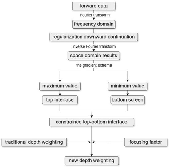
Figure 1.
Technical flow chart of the gravity focusing inversion based on attentional depth weighting using regularization of downward continuation.
3. Synthetic Studies
Two synthetic models—a “U”-shaped and a “Y”-shaped model—were employed to evaluate the performance of our proposed algorithm under different geological conditions. The “U”-shaped model simulates structurally complex, deformed, or metasomatized ore bodies, thereby testing the algorithm’s capability to accurately resolve intricate boundaries. In contrast, the “Y”-shaped model represents stratiform or block-shaped ore bodies, enabling an assessment of the algorithm’s effectiveness in distinguishing multiple density contrasts and their interactions. Together, these synthetic examples comprehensively validate the stability, adaptability, and practical efficacy of our method for imaging both regular and irregular mineral deposits.
3.1. “U”-Shaped Model
The subsurface is uniformly discretized into a 20 × 20 × 20 grid, yielding 8000 cells in total, and the “U”-shaped anomaly is embedded within this domain (Figure 2). The entire depth of the domain is 2000 m, subdivided into 20 cells of 100 m each; along the -axis, the domain extends 2000 m, with 20 cells of 100 m each; along the -axis, it spans 1000 m, divided into 20 cells of 50 m each. The “U” shape extends 600 m in depth, 800 m along , 500 m along , with a density of . The green-shaded area represents the horizontal reference plane, corresponding to the Earth’s surface, on which all observations and computations are based. This reference ensures consistency throughout the modeling and inversion processes, providing a uniform datum for accurate interpretation and comparison of gravity anomaly data. The chosen forward and inversion parameter is the component (Figure 3).
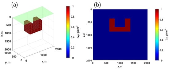
Figure 2.
Forward modeling results of “U”-shaped model; (a) 3D density model; (b) - cross-section at .
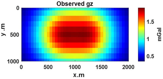
Figure 3.
Forward component field of “U”-shaped model.
3.2. Regularized Downward Continuation and Grid Resolution for “U”-Shaped Model
During forward data processing, the RCD is performed with the same grid division and spacing. Following this continuation, gradient calculations are carried out at each grid point to identify the anomaly’s top and bottom interfaces by locating gradient extrema. These extrema supply accurate input for subsequent depth weighting. Figure 4 presents a comparison among traditional depth weighting (Figure 4a), the RDC result (Figure 4b), and the integrated depth weighting combining RDC and traditional weighting (Figure 4c). The actual location of the synthetic model is indicated by the black rectangle. As illustrated, the application of RDC (Figure 4b) distinctly highlights the depth-weighted region, better aligning with the true position of the modeled anomaly. Furthermore, the integration of RDC with traditional depth weighting (Figure 4c) provides an enhanced and more focused representation of the model boundaries, improving inversion accuracy and clarity.
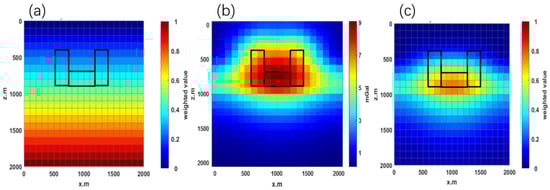
Figure 4.
Comparison of depth-weighting approaches: (a) traditional depth weighting; (b) the RDC result; and (c) combined weighting using traditional and RDC methods. The black rectangle outlines the true position of the ”U”-shaped model. Note that incorporating RDC distinctly highlights the depth weighting within the actual anomaly region, enhancing the precision of the subsequent inversion.
3.3. Inversion Configrations and Results for “U”-Shaped Model
The 3D inversion uses the same grid configuration as the forward model. The results and the corresponding - cross-section at y = 500 m are shown in Figure 5, allowing a direct comparison of different inversion strategies. One can see that the traditional focusing inversion exhibits limited accuracy when reconstructing some geological configurations, failing to approximate the true “U”-shaped model and showing a pronounced tailing effect (Figure 5a). In contrast, the proposed depth-weighted inversion based on regularized downward continuation restores the spatial position and geometry of the “U”-shaped model with high precision (Figure 5b), meets expected density standards, and significantly reduces the tailing phenomenon observed in the traditional approach. A Gaussian noise of 5% is introduced in Figure 5c. Compared to Figure 5b, the inversion results of the model with the added noise remain stable, demonstrating that the current algorithm exhibits a certain level of noise resistance.
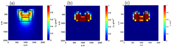
Figure 5.
Comparison of inversion results for ”U”-shaped model. (a) Inversion result using the traditional method; (b) inversion result using the proposed method; (c) inversion result of the proposed method with noise.
Figure 6 presents a comparison of convergence behaviors between the conventional and proposed inversion methods. The error fitting plot for the conventional method (Figure 6a) indicates that it reaches the predefined error threshold after 34 iterations. In contrast, the proposed method (Figure 6b) achieves the same error level within only 21 iterations. This comparison clearly demonstrates that the proposed method offers faster iterative convergence compared to the traditional approach.
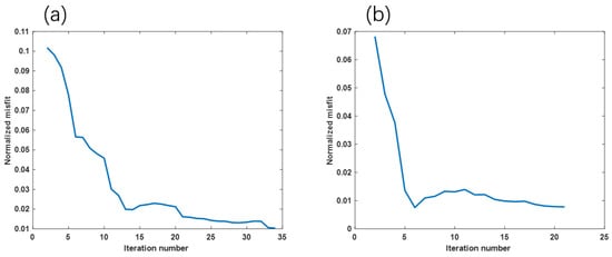
Figure 6.
Error comparison for ”U”-shaped model. (a) Error fitting plot using the traditional method; (b) Error fitting plot using the proposed method.
3.4. “Y”-Shaped Model
Model 2 uses the same 20 × 20 × 20 spatial grid as the “U”-shaped model but features a “Y”-shaped anomaly (Figure 7). The green region represents a segment of the actual terrain, with the surface assumed to be flat. This assumption is vital for both forward modeling and inversion analysis, as it ensures that all observation points and calculations are performed on a consistent horizontal reference plane. The “Y”-shaped model extends 600 m in depth, 1100 m along , 500 m along , with a density of . For both forward modeling and inversion, the component is employed (Figure 8).
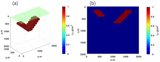
Figure 7.
Forward modeling results of “Y”-shaped model; (a) 3D density model; (b) - cross-section at .
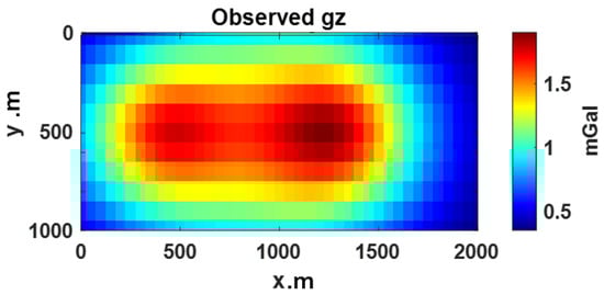
Figure 8.
Forward component field of “Y”-shaped model.
3.5. Regularized Downward Continuation and Grid Resolution for “Y”-Shaped Model
As in the “U”-shaped model, the RCD in the “Y”-shaped model is performed with the same grid division and spacing. Following this continuation, gradient calculations are carried out at each grid point to identify the anomaly’s top and bottom interfaces by locating gradient extrema. Figure 9 compares the effects of different depth-weighting strategies: (a) traditional depth weighting (Figure 9a); (b) the RDC result (Figure 9b); and (c) the combined approach integrating traditional depth weighting with RDC results (Figure 9c). The black rectangle denotes the actual model position. It is clear from the comparison that incorporating RDC significantly clarifies and enhances the depth-weighted regions, closely aligning the weighting distribution with the true anomaly location, particularly when employing the integrated approach (Figure 9c).
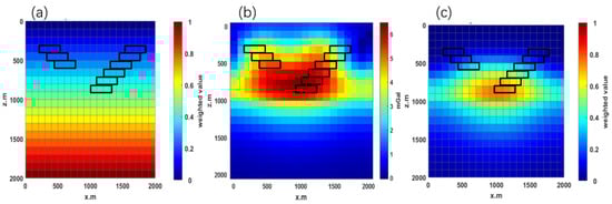
Figure 9.
Schematic comparison of depth weighting incorporating regularized downward continuation (RDC): (a) Traditional depth-weighting approach; (b) depth weighting derived from RDC; (c) integrated depth weighting obtained by combining traditional weighting with RDC results. The black rectangle indicates the actual location of the anomaly model.
3.6. Inversion Configrations and Results “Y”-Shaped Model
The 3D inversion uses the same grid configuration as the forward model. The results and the corresponding - cross-section at y = 500 m are shown in Figure 10, allowing a direct comparison of different inversion strategies. One can see that the traditional focusing inversion exhibits limited accuracy when reconstructing some geological configurations, failing to approximate the true “Y” shape and showing a pronounced tailing effect (Figure 10a). In contrast, the proposed depth-weighted inversion based on regularized downward continuation restores the spatial position and geometry of the “Y”-shaped model with high precision (Figure 10b), meets expected density standards, and significantly reduces the tailing phenomenon observed in the traditional approach. A Gaussian noise at a 5% level was introduced into the synthetic gravity data to assess the noise resilience of the proposed inversion method. Comparing the inversion result with the original noise-free scenario (Figure 10b), it can be observed that the shape, position, and amplitude of the recovered anomaly remain robust (Figure 9c). This indicates that the proposed inversion algorithm maintains satisfactory stability and demonstrates an effective resistance to typical data noise encountered in practical applications.
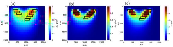
Figure 10.
Comparison of inversion results for “Y”-shaped model. (a) Inversion result using the traditional method; (b) inversion result using the proposed method; (c) inversion result of the proposed method with noise.
Figure 11 compares the convergence efficiency between the conventional inversion method and the proposed method. Figure 11a illustrates the error fitting curve for the conventional method, which achieves the predefined error threshold after approximately 130 iterations. In contrast, Figure 11b demonstrates the efficiency of the proposed inversion approach, reaching the same error level after just 30 iterations. This comparison highlights the significant improvement in convergence speed of the proposed method.
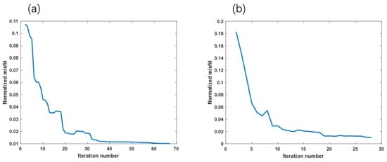
Figure 11.
Error comparison for ”Y”-shaped model. (a) Error fitting plot using the traditional method; (b) error fitting plot using the proposed method.
4. Case Study
4.1. Geological Background
The Dahongshan mining area lies in the southwestern portion of the iron–copper metallogenic belt in the Kangdian region, along the western boundary of the Yangtze Block in South China. Positioned within a triangular zone bordered by the Ailaoshan–Honghe and Luzhijiang faults, the deposit is hosted in metamorphosed volcano-sedimentary strata of the Paleoproterozoic Dahongshan Group. The main exposed rock units are the Paleoproterozoic Dahongshan Group and its overlying Mesozoic Triassic–Jurassic sedimentary cover [43]. In the southwestern part of the mining district, the Archean Beilaoshan Group melange, oriented northwest, is in disconformable contact with the overlying Dahongshan Group. From bottom to top, the Dahongshan Group is subdivided into the Laochanghe, Manganhe, Hongshan, Feiweihe, and Potou Formations [44].
Studies suggest that the earliest mafic intrusions in the Dahongshan region formed around 1.7 Ga, whereas mafic rocks dating to approximately 0.85 Ga likely represent a transitional stage of Neoproterozoic tectono-thermal events, during which evolving mafic magmatism facilitated the precipitation of copper and iron. Between 1.7 Ga and 0.85 Ga, the Kangdian region experienced multiple magmatic episodes, influenced by both the breakup of the Columbia supercontinent and the formation of Rodinia. Regional magmatic surveys indicate that from 1.75 to 1.70 Ga, a continental rift developed along the western margin of the Yangtze Block, featuring intense volcanic activity within rift basins and eventually transitioning into a passive continental margin—a process that continued beyond 1.50 Ga. Around 1.0 Ga, the assembly of the Rodinia supercontinent reunited the western Yangtze Block in the Kangdian tectonic zone, where the Luzhijiang fault is considered the suture created by ancient plate convergence. Along these suture faults, mantle-derived mafic–ultramafic magmas intruded, carrying extensive hydrothermal fluids that enriched regional deposits and altered the metallogenic environment.
Figure 12 shows the gravity anomaly field in the Dahongshan mining area [43], highlighting a pronounced positive Bouguer anomaly (Figure 12a). On the western side, the Honghe gravity gradient belt extends north–northwest, whereas a local low-gravity anomaly—Dibadu—appears in the north. The residual gravity anomalies, separated using the interpolation-cutting method proposed by Shizhe et al. [45], exhibit an east–west distribution with a maximum amplitude of up to 4 mGal (Figure 12b). The Bouguer gravity anomaly is computed from measured gravity data after correcting for topography, intermediate geological layers, elevation differences, and Earth’s normal gravity field using standard processing software. The residual gravity anomaly is subsequently derived by applying a filtering technique to the Bouguer gravity anomaly. Specifically, the filtering method applied in this study follows the approach of Shizhe et al. [45].
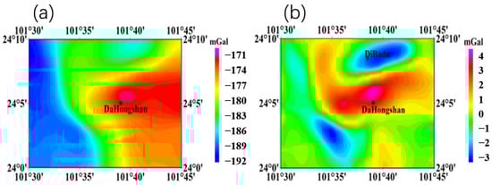
Figure 12.
Gravity anomaly map of the Dahongshan area. (a) Bouguer gravity anomaly; (b) residual gravity anomaly [46].
4.2. Inversion Configuration
According to Li et al. [46], inversion of regional gravity data in Dahongshan suggests a “U”-shaped deposit along an inclined basement structure, with large, lens-shaped ore bodies indicating a distinctive metallogenic framework. In this study, we applied regularized downward continuation RCD to the Dahongshan gravity data, maintaining the same horizontal spacing as in the original observation grid. Vertically, a continuation step of 1000 m was used for a total of 15 increments. After the continuation, gradient computations were performed in each - grid cell to delineate the geometry of the anomalous bodies. By analyzing gradient variations, maxima and minima were extracted to define the top and bottom boundaries of these anomalies (Figure 13).
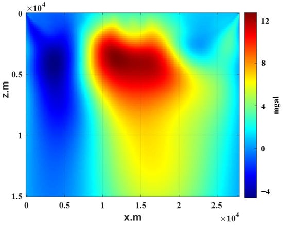
Figure 13.
Results of the regularized downward continuation along - cross-section at (the Dahongshan area).
Building upon this, gravity inversion was carried out in the Dahongshan area using the proposed depth-weighting method based on regularized downward continuation RDC. The inversion grid extends 27,655 m along the -axis (subdivided into 80 cells, each approximately 345 m), 20,040 m along the -axis (divided into 50 cells, each about 400 m), and 15,000 m in the -axis (partitioned into 15 cells of 1000 m). Figure 14 compares - cross-sectional inversion results from both the conventional approach and the proposed method. These results clearly show that the new method effectively mitigates the tailing artifacts seen in traditional inversions and significantly enhances focusing, leading to more accurate delineation of anomalous bodies. Additionally, the regions of higher density recovered by the inversion align well with earlier geological interpretations for Dahongshan, wherein low-density zones correspond to unmetamorphosed sedimentary cover, often composed of loosely consolidated clastic or carbonate materials.
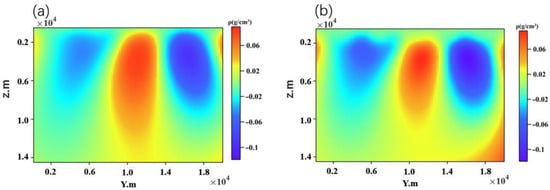
Figure 14.
Comparison of inversion results for the Dahongshan area. (a) Inversion result using the traditional method; (b) inversion result using the proposed method.
4.3. Inversion Results and Interpretation
Figure 15 presents the 3D inversion results, clearly illustrating the “U”-shaped anomalous intrusive body at depths ranging from approximately 4 to 5 km. Figure 16 further compares the predicted gravity anomaly field derived from inversion with the observed anomaly data. The close alignment between the two fields validates the effectiveness and reliability of the proposed inversion method when applied to actual gravity data from the Dahongshan area.
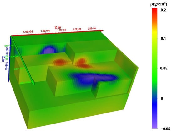
Figure 15.
Three-dimensional gravity inversion results in the Dahongshan area.
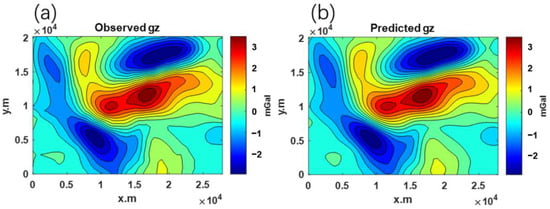
Figure 16.
Comparison of observed and predicted anomaly fields: (a) observed anomaly; (b) predicted anomaly.
Li et al. (2023) [46] previously conducted gravity inversion studies in the Dahongshan region, similarly identifying a significant intrusive body with a “U”-shaped geometry extending to about 6 km depth. Their research indicated that iron-rich ore bodies and mineralization in the area are predominantly controlled by basement tilting and fault structures, forming characteristic lens-shaped ore bodies. Building upon their findings, our proposed inversion method incorporates an attentional depth-weighting matrix, derived from regularized downward continuation results, which significantly enhances the imaging resolution and accuracy of subsurface density recovery. In particular, our approach improves clarity in delineating the boundaries and structural details of the intrusive anomaly, providing density amplitude estimations closer to actual geological conditions compared to the results presented by Li et al. (2023).
In addition, our approach reinforces the geological interpretation suggested by previous research, indicating that the gravity anomalies at deeper levels in Dahongshan are likely associated with residual intrusions of mantle-derived magmas, linked closely to early rift evolution and subsequent magmatic activity. This enhanced imaging precision offers critical new insights into the metallogenic processes and contributes to a more comprehensive understanding of the deep geological mechanisms responsible for ore formation in this region.
5. Discussion
The inversion framework introduced in this study, built upon the RDC, significantly enhances the resolution and accuracy of gravity inversion results. Unlike traditional methods, which apply uniform depth-weighting strategies and predominantly focus on central depths, our proposed attentional depth-weighting matrix explicitly targets the delineation of anomaly boundaries. This is accomplished by using RDC to suppress excessive high-frequency noise inherent in conventional DC, thereby stabilizing the extrapolation process. Subsequently, gradient extrema are computed within each grid cell, precisely identifying the upper and lower boundaries of subsurface anomalies. The spatial smoothing and local filtering procedures employed effectively reduce the influence of spurious extrema, resulting in stable and reliable anomaly boundary delineation.
By integrating this refined attentional depth-weighting matrix with conventional depth-weighting techniques and a minimum-support focusing factor, the proposed approach addresses common limitations of traditional methods, such as resolution deterioration at greater depths and ambiguity in defining anomaly interfaces. Moreover, optimization of gradient parameters and weighting strategies further improves sensitivity towards deep or subtle anomalies. Nevertheless, some inherent limitations remain. The proposed method requires increased computational effort due to the integration of RDC and the construction of the attentional matrix, highlighting the need for future computational efficiency optimizations. Furthermore, accurate boundary delineation in extremely complex geological scenarios may be challenging, underscoring the necessity of incorporating complementary geophysical datasets and geological constraints to enhance anomaly characterization and inversion reliability.
6. Conclusions
High-precision gravity inversion is crucial for resolving subsurface structures in mineral exploration and geological research. Beyond locating ore bodies and delineating tectonic features, accurate inversion can guide cost-effective drilling strategies, reduce exploration risks, and deepen our understanding of crustal processes. To address the inherent shortcomings of traditional methods—including amplified noise at depth, inadequate preservation of anomaly boundaries, and uniform depth weighting—this study proposes a novel approach involving two main innovations: (1) integration of RDC to stabilize noise amplification inherent in potential field extrapolation, and (2) introduction of an attentional depth-weighting matrix to effectively delineate anomaly boundaries.
The proposed inversion framework is fundamentally built on an RDC technique, which projects surface gravity data downward to highlight deeper anomalies while effectively suppressing high-frequency noise amplification inherent in conventional DC. Following RDC, gradient extrema are identified within each grid cell to accurately delineate the top and bottom boundaries of anomalous bodies. To reduce the influence of spurious extrema, spatial smoothing and local filtering procedures are applied, enhancing boundary stability. These refined boundaries form the basis for constructing an attentional depth-weighting matrix, which is subsequently integrated with a traditional depth-weighting matrix and a minimum-support focusing factor. The proposed attentional depth-weighting matrix, derived from the RDC approach, effectively addresses the resolution deterioration commonly experienced by traditional depth-weighting methods at greater depths. By incorporating gradient extrema analysis, our method precisely delineates the upper and lower boundaries of subsurface anomalies, significantly enhancing the resolution and interpretability of deep structures. Additionally, the RDC mechanism effectively mitigates high-frequency noise amplification, reducing instability caused by shallow interference and measurement errors. Consequently, the integrated method ensures a clearer depiction of anomaly boundaries and improves overall inversion accuracy, making it highly suitable for detailed subsurface geological analyses. Additionally, gradient parameters and weighting strategies are optimized to ensure improved sensitivity toward weak or deep anomalies. Although inherent limitations remain, employing multi-scale analyses and incorporating geological constraints can significantly enhance anomaly characterization and improve the interpretability of inversion results.
The proposed method effectively suppresses shallow sensitivity and accurately recovers deeper targets with amplitudes closely matching those of the two synthetic models. Applied to actual data from the Dahongshan mining region, the resulting inversion captures high-density intrusive bodies at depths of approximately 4–5 km, revealing their characteristic “U” shape. These findings underscore the method’s ability to illuminate significant deep anomalies while preserving their boundaries, offering new insights into complex geological settings.
Nonetheless, the approach still has certain limitations. First, combining RDC with the construction of an attentional depth-weighting matrix inevitably increases computational complexity, making it more resource-intensive than conventional inversion techniques. Further optimization is therefore needed to enhance computational efficiency, especially for large-scale datasets. Second, although our algorithm has shown promising results in both synthetic models and practical applications in the Dahongshan area, its general applicability across diverse geological contexts has yet to be confirmed. Highly intricate geological structures may pose challenges for accurate boundary delineation, emphasizing the importance of integrating complementary geophysical data to improve geological constraints and bolster the reliability of inversion outcomes.
Author Contributions
Conceptualization, Z.X.; Methodology, Z.X.; Algorithm, Z.Q., M.X., Y.Z. and A.S.; Validation, Z.X. and J.L.; Formal analysis, M.X.; Investigation, Z.Q. and J.L.; Resources, J.L.; Data curation, M.X., Y.Z. and A.S.; Writing—original draft, Z.Q.; Writing—review & editing, Z.X.; Supervision, G.M.; Project administration, G.M.; Funding acquisition, G.M. All authors have read and agreed to the published version of the manuscript.
Funding
This research was funded by the Natural Science Foundation of Sichuan Province under grant number 2024NSFSC0079.
Data Availability Statement
The data presented in this study are available on request from the corresponding author due to the confidentiality agreement stipulated by the data.
Conflicts of Interest
The authors declare no conflict of interest.
References
- Kamm, J.; Lundin, I.A.; Bastani, M.; Sadeghi, M.; Pedersen, L.B. Joint inversion of gravity, magnetic, and petrophysical data—A case study from a gabbro intrusion in Boden, Sweden. Geophysics 2015, 80, B131–B152. [Google Scholar] [CrossRef]
- Hu, Y.; Wei, X.; Wu, X.; Sun, J.; Huang, Y.; Chen, J. Three-dimensional cooperative inversion of airborne magnetic and gravity gradient data using deep-learning techniques. Geophysics 2024, 89, WB67–WB79. [Google Scholar] [CrossRef]
- Zhdanov, M.S. Inverse Theory and Applications in Geophysics; Elsevier: Amsterdam, The Netherlands, 2015; Volume 36. [Google Scholar]
- Zhou, S.; Wei, Y.; Lu, P.; Jiao, J.; Jia, H. Deep-Learning Gravity Inversion Method with Depth-Weighting Constraints and Its Application in Geothermal Exploration. Remote Sens. 2024, 16, 4467. [Google Scholar] [CrossRef]
- Fan, D.; Li, S.; Li, X.; Yang, J.; Wan, X. Seafloor topography estimation from gravity anomaly and vertical gravity gradient using nonlinear iterative least square method. Remote Sens. 2020, 13, 64. [Google Scholar] [CrossRef]
- Zhang, S.; Andersen, O.B.; Kong, X.; Li, H. Inversion and validation of improved marine gravity field recovery in South China Sea by incorporating HY-2A altimeter waveform data. Remote Sens. 2020, 12, 802. [Google Scholar] [CrossRef]
- Gallardo, L.A.; Fontes, S.L.; Meju, M.A.; Buonora, M.P.; De Lugao, P.P. Robust geophysical integration through structure-coupled joint inversion and multispectral fusion of seismic reflection, magnetotelluric, magnetic, and gravity images: Example from Santos Basin, offshore Brazil. Geophysics 2012, 77, B237–B251. [Google Scholar] [CrossRef]
- Alencar de Matos, C.; Mendonça, C.A. Poisson magnetization-to-density-ratio and magnetization inclination properties of banded iron formations of the Carajás mineral province from processing airborne gravity and magnetic data. Geophysics 2020, 85, K1–K11. [Google Scholar] [CrossRef]
- Morgan, J.P.; Blackman, D.K. Inversion of combined gravity and bathymetry data for crustal structure: A prescription for downward continuation. Earth Planet. Sci. Lett. 1993, 119, 167–179. [Google Scholar] [CrossRef]
- Vaníček, P.; Sun, W.; Ong, P.; Martinec, Z.; Najafi, M.; Vajda, P.; Ter Horst, B. Downward continuation of Helmert’s gravity. J. Geodesy 1996, 71, 21–34. [Google Scholar] [CrossRef]
- Novák, P.; Heck, B. Downward continuation and geoid determination based on band-limited airborne gravity data. J. Geodesy 2002, 76, 269–278. [Google Scholar] [CrossRef]
- Tóth, G.; Földvári, L.; Tziavos, I.N.; Ádám, J. Upward/downward continuation of gravity gradients for precise geoid determination. Acta Geod. Geophys. Hung. 2006, 41, 21–30. [Google Scholar] [CrossRef]
- Wang, X.; Xia, Z.; Shi, P.; Sun, Z. A comparison of different downward continuation methods for airborne gravity data. Chin. J. Geophys 2004, 47, 1143–1149. [Google Scholar] [CrossRef]
- Ma, G.; Niu, Y.; Li, L.; Li, Z.; Meng, Q. Adaptive Space–Location-Weighting Function Method for High-Precision Density Inversion of Gravity Data. Remote Sens. 2023, 15, 5737. [Google Scholar] [CrossRef]
- Ming, Y.; Ma, G.; Wang, T.; Ma, B.; Meng, Q.; Li, Z. Power-Type Structural Self-Constrained Inversion Methods of Gravity and Magnetic Data. Remote Sens. 2024, 16, 681. [Google Scholar] [CrossRef]
- Liu, B.; Bian, S.; Ji, B.; Wu, S.; Xian, P.; Chen, C.; Zhang, R. Application of the Fourier Series Expansion Method for the Inversion of Gravity Gradients using Gravity Anomalies. Remote Sens. 2022, 15, 230. [Google Scholar] [CrossRef]
- Martinez, C.; Li, Y.; Krahenbuhl, R.; Braga, M. 3D Inversion of airborne gravity gradiomentry for iron ore exploration in Brazil. In Proceedings of the SEG International Exposition and Annual Meeting, Denver, CO, USA, 17–22 October 2010; p. SEG-2010-1753. [Google Scholar]
- Zhdanov, M.S.; Lin, W. Adaptive multinary inversion of gravity and gravity gradiometry data. Geophysics 2017, 82, G101–G114. [Google Scholar] [CrossRef]
- Zhang, R.; Zhang, L.; Li, T.; Liu, C.; He, H.; Deng, X. Gravity inversion with a binary structure constraint imposed by magnetotelluric data and its application to a Carlin-type gold deposit. Geophysics 2023, 88, K39–K50. [Google Scholar] [CrossRef]
- Xian, M.; Xu, Z.; Zhdanov, M.S.; Ding, Y.; Wang, R.; Wang, X.; Li, J.; Zhao, G. Recovering 3D Salt Dome by Gravity Data Inversion Using ResU-Net++. Geophysics 2024, 89, G93–G108. [Google Scholar] [CrossRef]
- Lü, Q.; Qi, G.; Yan, J. 3D geologic model of Shizishan ore field constrained by gravity and magnetic interactive modeling: A case history. Geophysics 2013, 78, B25–B35. [Google Scholar] [CrossRef]
- Zhou, J.; Meng, X.; Guo, L. An efficient cross-gradient joint inversion algorithm of gravity and magnetic data with depth weighting and bound constraints. In Proceedings of the International Workshop and Gravity, Electrical & Magnetic Methods and their Applications, Chenghu, China, 19–22 April 2015; pp. 84–87. [Google Scholar]
- Wu, G.; Wei, Y.; Dong, S.; Zhang, T.; Yang, C.; Qin, L.; Guan, Q. Improved Gravity Inversion Method Based on Deep Learning with Physical Constraint and Its Application to the Airborne Gravity Data in East Antarctica. Remote Sens. 2023, 15, 4933. [Google Scholar] [CrossRef]
- Bai, Z.; Wang, Y.; Wang, C.; Yu, C.; Lukyanenko, D.; Stepanova, I.; Yagola, A.G. Joint Gravity and Magnetic Inversion Using CNNs’ Deep Learning. Remote Sens. 2024, 16, 1115. [Google Scholar] [CrossRef]
- Ma, G.; Gao, T.; Li, L.; Wang, T.; Niu, R.; Li, X. High-Resolution Cooperate Density-Integrated Inversion Method of Airborne Gravity and Its Gradient Data. Remote Sens. 2021, 13, 4157. [Google Scholar] [CrossRef]
- Vitale, A.; Fedi, M. Self-constrained inversion of potential fields through a 3D depth weighting. Geophysics 2020, 85, G143–G156. [Google Scholar] [CrossRef]
- Li, Y.; Oldenburg, D.W. 3-D inversion of magnetic data. Geophysics 1996, 61, 394–408. [Google Scholar] [CrossRef]
- Li, Y.; Oldenburg, D.W. 3-D inversion of gravity data. Geophysics 1998, 63, 109–119. [Google Scholar] [CrossRef]
- Sun, J.; Li, Y. Adaptive L p inversion for simultaneous recovery of both blocky and smooth features in a geophysical model. Geophys. J. Int. 2014, 197, 882–899. [Google Scholar] [CrossRef]
- Liang, S.; Wang, X.; Xu, Z.; Dai, Y.; Wang, Y.; Guo, J.; Jiao, Y.; Li, F. Steep subduction of the Indian continental mantle lithosphere beneath the eastern Himalaya revealed by gravity anomalies. Sci. China Earth Sci. 2023, 66, 1994–2010. [Google Scholar] [CrossRef]
- Wei, X.; Li, K.; Sun, J. Mapping critical mineral resources using airborne geophysics, 3D joint inversion and geology differentiation: A case study of a buried niobium deposit in the Elk Creek carbonatite, Nebraska, USA. Geophys. Prospect. 2023, 71, 1247–1266. [Google Scholar] [CrossRef]
- He, H.; Li, T.; Zhang, R. Joint inversion of 3D gravity and magnetic data under undulating terrain based on combined hexahedral grid. Remote Sens. 2022, 14, 4651. [Google Scholar] [CrossRef]
- Li, Z.; Yao, C. An investigation of lp-Norm minimization for the artifact-free inversion of gravity data. Remote Sens. 2023, 15, 3465. [Google Scholar] [CrossRef]
- Li, Z.; Guo, J.; Ji, B.; Wan, X.; Zhang, S. A review of marine gravity field recovery from satellite altimetry. Remote Sens. 2022, 14, 4790. [Google Scholar] [CrossRef]
- Zhdanov, M.S. Geophysical Inverse Theory and Regularization Problems; Elsevier: Amsterdam, The Netherlands, 2002; Volume 36. [Google Scholar]
- Xu, Z.; Zou, G.; Wei, Q.; Tian, J.; Yuan, H. Focusing joint inversion of gravity and magnetic data using a clustering stabilizer in a space of weighted parameters. Geophys. J. Int. 2021, 224, 1344–1359. [Google Scholar] [CrossRef]
- Xu, Z.; Zhdanov, M.S. Three-dimensional Cole-Cole model inversion of induced polarization data based on regularized conjugate gradient method. IEEE Geosci. Remote Sens. Lett. 2015, 12, 1180–1184. [Google Scholar] [CrossRef]
- Xu, Z.; Wan, L.; Han, M.; Zhdanov, M.S.; Mao, Y. Joint inversion of gravity gradiometry data by model-weighted clustering in logarithmic space. In Proceedings of the SEG International Exposition and Annual Meeting, San Antonio, TX, USA, 15–20 September 2019; p. D023S012R006. [Google Scholar]
- Commer, M. Three-dimensional gravity modelling and focusing inversion using rectangular meshes. Geophys. Prospect. 2011, 59, 966–979. [Google Scholar] [CrossRef]
- Zhang, Z.; Fan, J.; Bai, Y.; Dong, D. Joint inversion of gravity-magnetic-seismic data of a typical profile in the China Sea-Western Pacific area. Chin. J. Geophys 2018, 61, 2871–2891. [Google Scholar] [CrossRef]
- Martin, R.; Monteiller, V.; Komatitsch, D.; Perrouty, S.; Jessell, M.; Bonvalot, S.; Lindsay, M. Gravity inversion using wavelet-based compression on parallel hybrid CPU/GPU systems: Application to southwest Ghana. Geophys. J. Int. 2013, 195, 1594–1619. [Google Scholar] [CrossRef]
- Tikhonov, A.N.; Arsenin, V.I. Solutions of Ill-Posed Problems; Winston: Washington, DC, USA, 1977; Volume 14. [Google Scholar]
- Greentree, M.R.; Li, Z. The oldest known rocks in south–western China: SHRIMP U–Pb magmatic crystallisation age and detrital provenance analysis of the Paleoproterozoic Dahongshan Group. J. Asian Earth Sci. 2008, 33, 289–302. [Google Scholar] [CrossRef]
- Zhao, X.; Zhou, M.; Su, Z.; Li, X.; Chen, W.; Li, J. Geology, geochronology, and geochemistry of the Dahongshan Fe-Cu-(Au-Ag) deposit, Southwest China: Implications for the formation of iron oxide copper-gold deposits in intracratonic rift settings. Econ. Geol. 2017, 112, 603–628. [Google Scholar] [CrossRef]
- Shizhe, X.; Yan, Z.; Baihong, W.; Hu, Y.; Changfu, Y. The application of cutting method to interpretation of magnetic anomaly in region of Ludong. Geophys. Prospect. Pet. 2006, 45, 316. [Google Scholar] [CrossRef]
- Li, J.; Xu, Z.; Jian, X.; Li, M.; Li, J.; Wang, X. Gravity and magnetic focusing inversion in revealing the metallogenic pattern of Dahongshan Copper–Iron deposit in the Kangdian Area, China. IEEE Trans. Geosci. Remote Sens. 2023, 61, 4501110. [Google Scholar] [CrossRef]
Disclaimer/Publisher’s Note: The statements, opinions and data contained in all publications are solely those of the individual author(s) and contributor(s) and not of MDPI and/or the editor(s). MDPI and/or the editor(s) disclaim responsibility for any injury to people or property resulting from any ideas, methods, instructions or products referred to in the content. |
© 2025 by the authors. Licensee MDPI, Basel, Switzerland. This article is an open access article distributed under the terms and conditions of the Creative Commons Attribution (CC BY) license (https://creativecommons.org/licenses/by/4.0/).