1. Introduction
Soil organic matter (SOM) is an active and critical component of the soil carbon pool, and its spatial distribution characteristics are of great significance for revealing regional soil quality and global carbon cycling processes [
1]. However, due to the combined effects of structural and stochastic factors, the spatial distribution of SOM exhibits significant variability and non-stationarity, causing significant uncertainty in modeling and quantitatively describing its spatial variation process [
2]. Therefore, although it is necessary to accurately obtain spatial distribution information on regional SOM, many challenges remain in practical operation.
In hilly basin areas, the topographic conditions are highly variable. There are distinct differences in lighting, heat, and moisture conditions among different topographic positions, endowing these regions with a high degree of spatial heterogeneity. The influencing factors are intricate and complex, rendering it particularly challenging to quantitatively describe the soil morphology, properties, their process variations, and spatial correlations [
3]. Therefore, digital soil mapping (DSM) has been widely used in recent years as an important technology for quickly and accurately determining the spatial distribution of regional soil attributes [
3]. However, due to the combined influence of natural soil-forming factors and human activities, the SOM in farmland often exhibits significant spatial non-stationarity, which further increases the difficulty of SOM spatial prediction [
4]. Identifying the key influencing factors of the SOM spatial distribution and introducing them into prediction models can greatly improve prediction accuracy.
Traditional soil attribute mapping methods include Kriging interpolation, inverse distance weight interpolation, spline function interpolation, and other geostatistical methods [
5]. Ordinary Kriging (OK) is the most widely adopted Kriging method, celebrated for its model simplicity and capacity to generate unbiased optimal predictions alongside uncertainty quantification [
6].
As well as the commonly used Kriging and regression analysis methods, researchers often use linear estimation methods, which present difficulty in capturing the complex nonlinear relationship between SOM and environmental variables [
6]. Therefore, in recent years, an increasing number of scholars have begun to introduce machine learning algorithms, such as support vector machines (SVMs), random forests (RFs), artificial neural networks (ANNs), and regression trees, aiming to more accurately establish the nonlinear relationship between SOM and environmental variables [
7,
8]. These methods typically rely on sample data and environmental covariates for fitting, with the commonly used environmental variables including soil type, climate factors, land use type, vegetation index, terrain factors, and soil parent material [
9,
10]. Terrain factors in particular have a significant impact on SOM content by regulating surface runoff, solar radiation, soil erosion, moisture content, and temperature, making them particularly important in hilly and mountainous areas [
11].
The random forest (RF) model, emerging in recent years, is a tree-structured model that adopts an ensemble learning strategy. It can be used for both classification and the prediction of continuous variables. It constructs a series of tree models and allows them to be trained and make predictions independently. The final prediction result is determined by voting among the prediction results of all trees (for categorical prediction) or by taking the average (for numerical prediction). Therefore, it exhibits excellent robustness [
12]. In addition, RF can display the relative importance of each environmental variable in the modeling process (using the % IncMSE index). Owing to its outstanding prediction accuracy and good interpretability, RF has become one of the most commonly used machine learning algorithms in recent years.
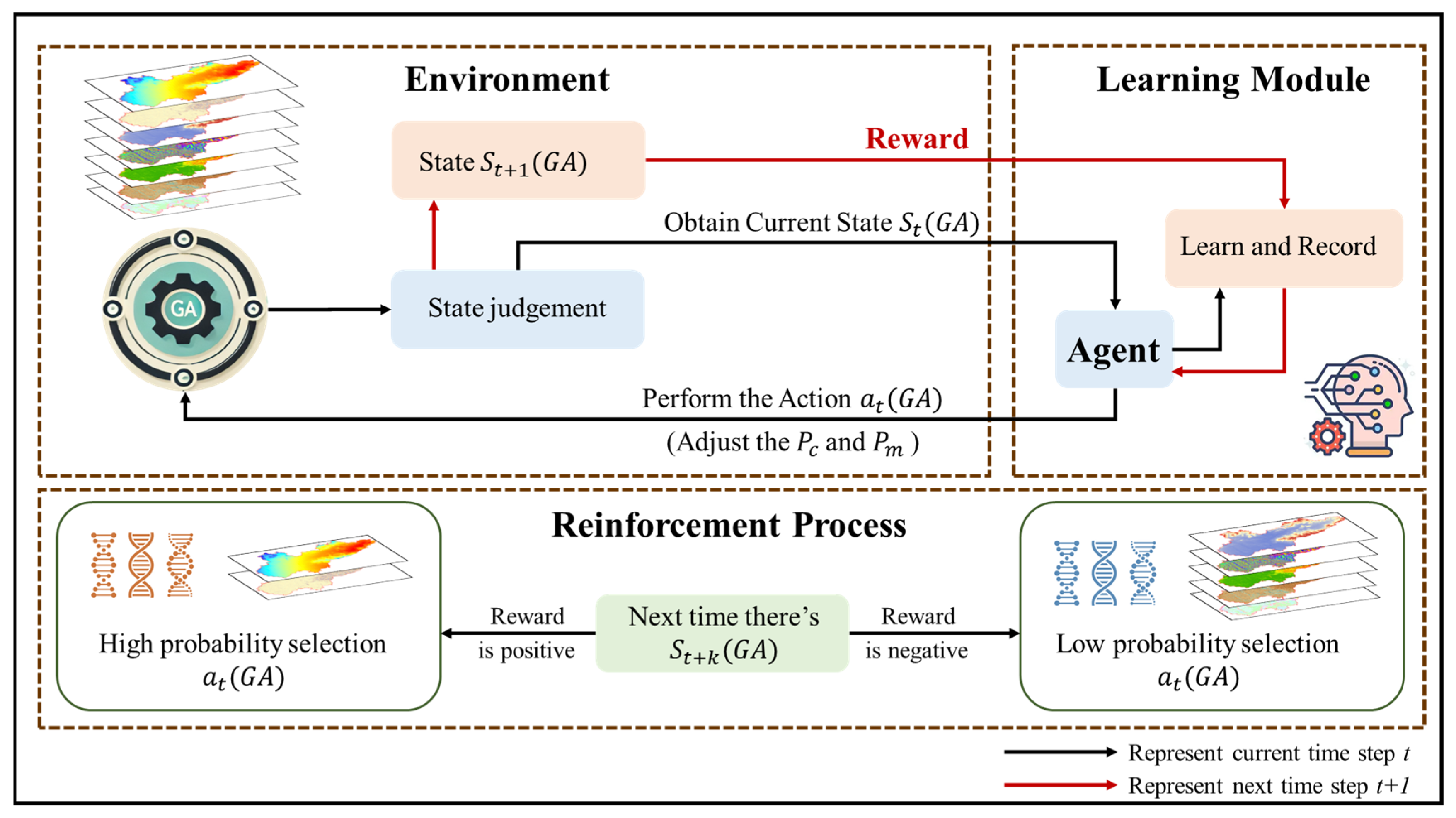
In digital soil mapping, the selection of environmental variables is one of the crucial steps which directly influences the spatial distribution of soil properties and the accuracy of prediction models. Therefore, numerous scholars have dedicated themselves to researching how to screen out the factors that have the greatest impact on soil properties from a multitude of environmental variables. To endow the model with high prediction accuracy, it is necessary to conduct an efficient screening process from a large number of feature variables. This involves selecting the optimal subset of features and avoiding multicollinearity to enhance the model’s prediction accuracy and simplify its complexity. The genetic algorithm (GA) is a global optimization algorithm that simulates the natural evolution process, continuously optimizing variable combinations through operations such as selection, crossover, and mutation in order to select feature sets that can maximize model performance [
13]. In complex terrain and multivariate environments, the GA can effectively avoid becoming stuck in local optima, thereby improving the robustness and accuracy of model predictions [
14]. However, the random forest model based on GA filtering features (GA-RF) has not been fully applied in SOM estimation in complex areas, and its advantages in SOM prediction over the RF model using full-variable prediction still need to be verified. Therefore, this study proposes a random forest model based on the genetic algorithm for variable combination optimization, aiming to improve the prediction accuracy of the SOM spatial distribution in complex regions and provide new perspectives and methods for DSM research.
Although machine learning methods typically outperform traditional statistical methods in terms of prediction accuracy, their “black box” nature—i.e., their lack of sufficient interpretability—has always limited their practical applications. To address this issue, the SHAP (Shapley Additive Explanations) method based on game theory and local interpretation theory was introduced to quantitatively estimate the contribution of each feature variable to the model’s prediction results [
15]. In the field of soil property simulation, SHAP has not only successfully identified key driving factors but has also effectively analyzed the interactions between different climate and terrain variables, making it widely used to interpret the prediction results of complex models [
9,
16].
Lanxi City is the largest Yangmei-producing area in the region, with a typical hilly and basin landform. Identifying the main controlling factors of the SOM in farmland in Lanxi City and obtaining a high-precision SOM spatial distribution map will help not only formulate scientific and reasonable farmland planting and management strategies, optimize land use layouts, increase soil carbon sequestration capacities, and alleviate the greenhouse effect but also enhance soil fertility and achieve increased grain production.
The main objectives of this study are to (1) explore the potential application of GA-RF models based on variable combination optimization in DSM in complex regions; (2) evaluate the performance differences between this model and the ordinary Kriging method (OK) and the RF model based on full-variable prediction in terms of predicting the SOM spatial distribution; and (3) use the SHAP method to analyze the spatial correlation between SOM formation environmental variables and SOM content.
3. Experimental Results and Analysis
3.1. Basic Statistics of Soil Organic Matter Content
The distribution characteristics and variability of data have an impact on the reliability of spatial interpolation results. In Kriging interpolation, if the data follow a normal distribution, the optimal prediction results can be obtained [
31]. Therefore, normality testing and transformation of the data were performed to obtain more reliable prediction results.
This study first conducted descriptive statistics on the soil organic matter content of the training and test sets, and it performed K-S tests on the experimental data in SPSS 26. The results (
Table 2) show that the maximum value (Max), minimum value (Min), average value (AVE), and standard deviation (SD) of the training and test sets were relatively consistent. The magnitude of the coefficient of variation (CV) indicates the spatial variability of soil properties. When the coefficient of variation is less than 10%, it suggests weak variability; when the coefficient of variation is greater than 100%, it suggests strong variability. A value between the two suggests moderate variability. According to
Table 2, the results indicate that the soil organic matter content at the sampling points ranges from 3.91 to 66.20 g/kg, with a relatively large standard deviation. This suggests that there are fluctuations of varying degrees in the soil organic matter content among local areas within the study region. The coefficient of variation for the training set and the test set is 37.77% and 38.15% respectively, indicating that the soil organic matter in the study area belongs to a moderately variable type.
Based on the skewness and kurtosis values, as well as the K-S value (K-S) test results, it could be concluded that both the training and test sets are non-normally distributed. Although Kriging interpolation does not strictly require data to be normally distributed, when the data deviate too far from the normal distribution, the interpolation effect may not be ideal. After performing Box–Cox transformation (Box–Cox) on the training and test sets, the skewness and kurtosis values were close to 0, and the K-S test results were greater than 0.05, thus conforming to the normal distribution.
3.2. Assessment of the Importance of Environmental Variables in RF Models
The optimal parameters of the random forest model were determined by applying the grid-search method [
32]. Grid-search functions by exhaustively exploring all possible combinations within a pre-defined hyperparameter range to identify the optimal hyperparameter configuration. Although this method can efficiently identify a relatively favorable hyperparameter setting, it usually requires substantial computational resources and time. In the preliminary experimental stage, the hyperparameter ranges for the grid-search were carefully determined based on insights from previous academic literature and empirical tests. For both the RF and RFGA models, the range of mtry (the number of variables randomly sampled as candidates at each split) was set from 1 to 20. This decision was made because different values of mtry can significantly impact the model’s generalization ability. The range of ntree (the number of trees in the forest) was set from 100 to 1000. This is because increasing the number of trees can improve the model’s performance up to a certain point, after which the marginal improvement becomes negligible while the computational cost increases. To select the optimal hyperparameters, we used the root-mean-square error (RMSE) calculated on an independent validation set as the evaluation metric. After conducting the grid-search, the optimal parameters for the RF model in this study were determined to be mtry = 19 and ntree = 500. For the RFGA model, the optimal parameters were found to be mtry = 4 and ntree = 500.
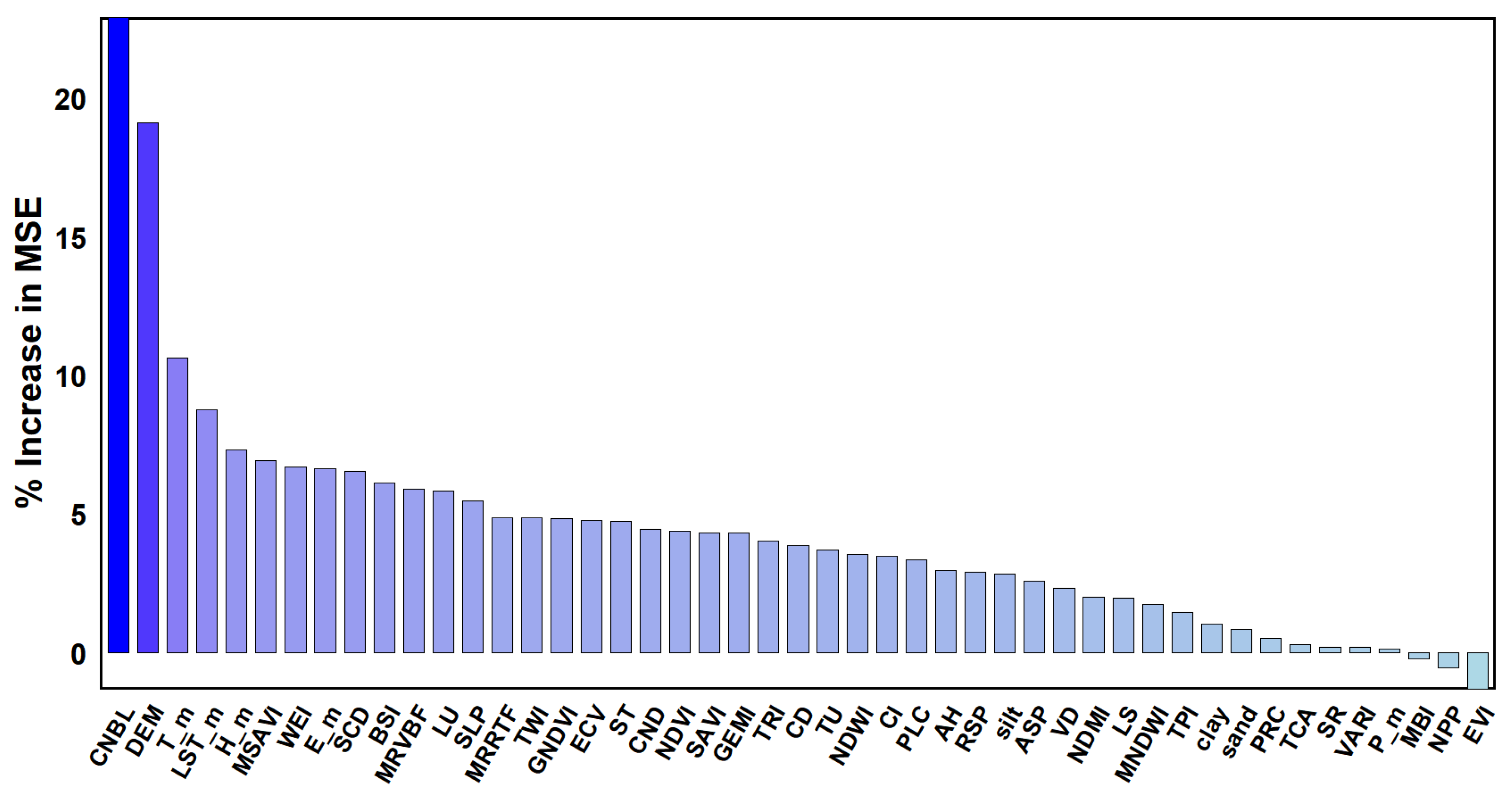
Based on the RF model, the importance ranking of all environmental variables involved in modeling was conducted, and it was found that there were differences in the importance of the effects of the different environmental variables on the prediction results of different attribute spaces. In the RF model importance evaluation results (% IncMSE) of the soil SOM content, the order of influence on the SOM from high to low was as follows (
Figure 3): the CNBL, DEM, T_m, LSTM_m, H_m, MSAVI, WEI, E_m, SCD, BSI, etc.
Therefore, the two topographic factors that had the greatest impact on the SOM in the RF results were the CNBL and DEM. The core distinction between CNBL and DEM lies in the fact that the former serves as a dynamic geomorphic evolution reference, whereas the latter represents static topographic data. By controlling erosion, sedimentation, and hydrological processes, CNBL indirectly yet profoundly influences the spatial distribution and stability of soil organic matter, making it a critical parameter for understanding watershed-scale carbon cycling.
The three biological factors that had the greatest impact on the SOM in the RF results were the T_m, LSTM_m and H_m. T_m determines decomposition rates across climatic zones (e.g., rapid turnover in tropics vs. slow accumulation in cold regions), drives freeze–thaw cycles releasing stored organic carbon, and shapes microbial adaptation. LST_m directly drives near-surface SOM mineralization (Q10 effect), with elevated temperatures increasing decomposition rates but drought potentially limiting microbial activity; it also influences vegetation distribution. H_m regulates SOM through microbial activity, plant productivity, and leaching: high humidity accelerates aerobic decomposition but slows anaerobic decay, while optimal moisture enhances plant carbon inputs.
3.3. Analysis of the Accuracy of OK, RF, and RF-GA Models
In this study, soil organic matter sample point data were utilized. Kriging, random forest, and random forest with variable screening were employed to predict the spatial distribution of soil organic matter and evaluate the accuracy. First, the dataset was partitioned into a training set and a validation set at an 8:2 ratio. The former was used for model construction, while the latter was used to assess the generalization ability of the model. Kriging constructed the model by calculating the variogram and evaluated the accuracy with the validation set. The random forest method sampled subsets from the training set to construct multiple decision trees, and after training, the validation set was used for evaluation. For the random forest with variable screening, variables were screened first, and then the model was constructed, predicted, and evaluated in the same way. This was carried out to compare the advantages and disadvantages of each method.
After obtaining the SOM (Box–Cox transformation) spatial prediction results of each prediction model, inverse transformation can be used to obtain the SOM spatial distribution results based on Kriging interpolation. RF uses 47 full variables to predict soil organic matter across the entire domain.
The selection of environmental variables for GA-RF relies on the genetic algorithm. Inspired by evolution, it encodes variables as chromosomes. Starting with a random population, it assesses chromosomes via fitness functions. Through selection, crossover and mutation, it pursues optimal model performance. After meeting termination criteria, it outputs the best variable combo. The optimal variable combination selected by GA-RF is P_m, E_m, VARI, NDWI, NPP, MNDWI, GNDVI, BSI, AH, ASP, CI, CNBL, CND, DEM, LS, MRRTF, RSP, TCA, LU, ST, and SCD, predicting soil SOM across the entire region based on 21 environmental variables.
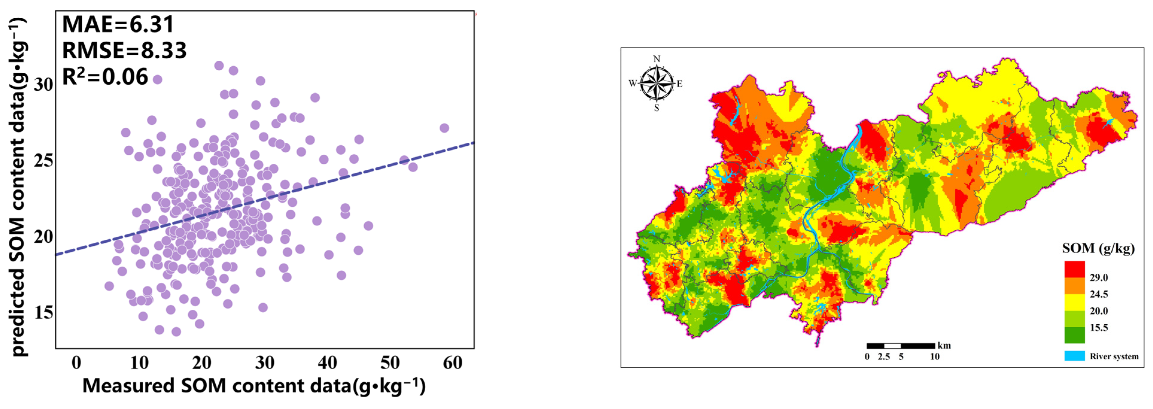
The prediction results of each model are externally validated using the MAE, RMSE, R
2, and LCCC, as shown in
Table 3. It can be observed that, among the three types of prediction models, the OK model has higher MAE (6.31) and RMSE (8.33) values, while R
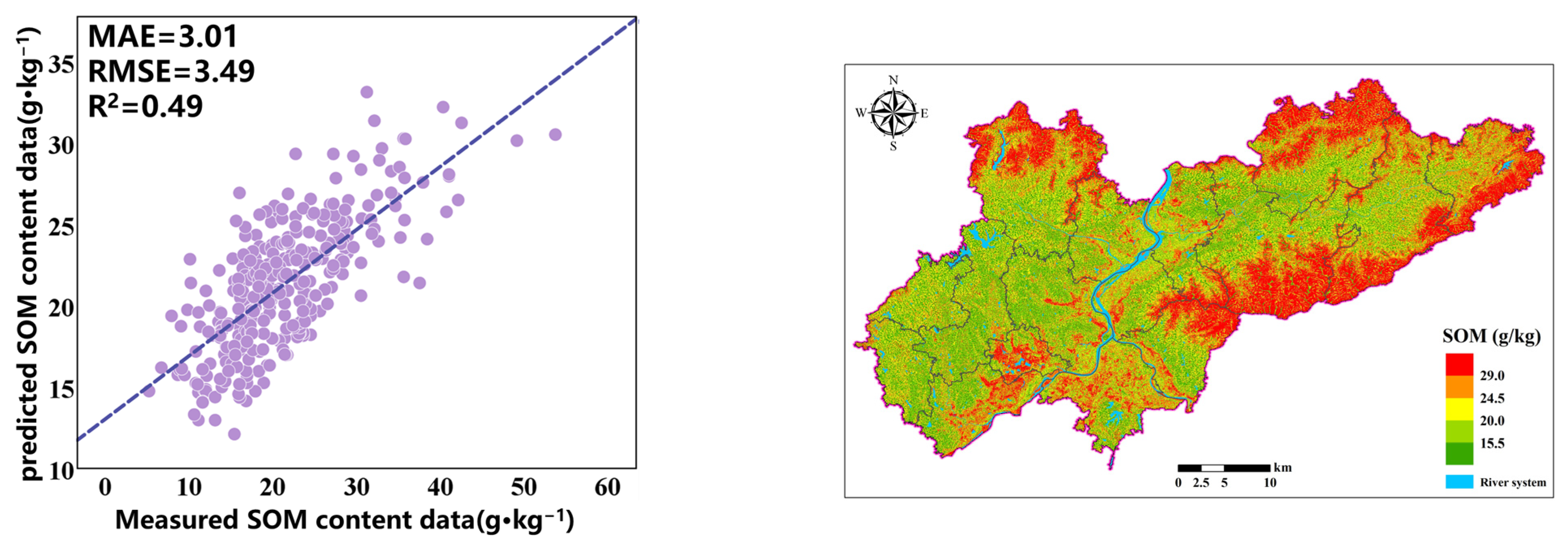
2 (0.06) and LCCC (0.16) are very low, indicating that using only the Kriging method results in poor prediction accuracy and trends. The RF + GA model exhibits a relatively high R
2 (0.49) and LCCC (0.67), along with low MAE (3.02) and RMSE (3.49). In the regression model, according to the LCCC results, the order from best to worst for each model is RF-GA (0.67) > RF (0.38) > OK (0.16). Compared with the OK model and the RF model, the R
2 of the RF + GA model has increased by 0.43 and 0.28, respectively. These results indicate that the RF-GA model considering nonlinear relationships has the smallest spatial interpolation error, OK has the largest spatial interpolation error, and RF-GA and RF have improved interpolation accuracy compared to OK due to the use of auxiliary variables. The RF-GA model is the optimal SOM prediction model in this study.
3.4. SHAP Overlay Explanation
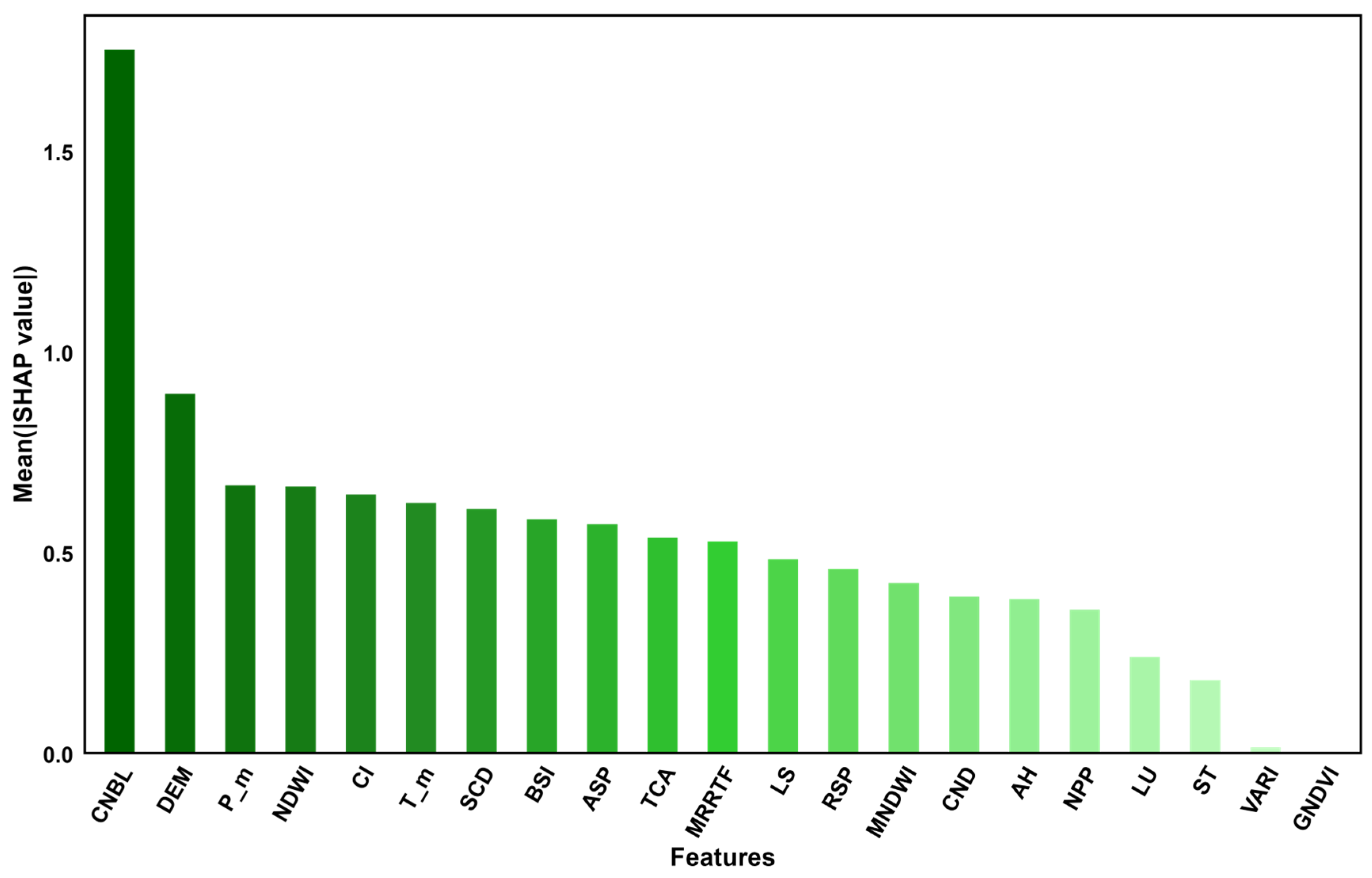
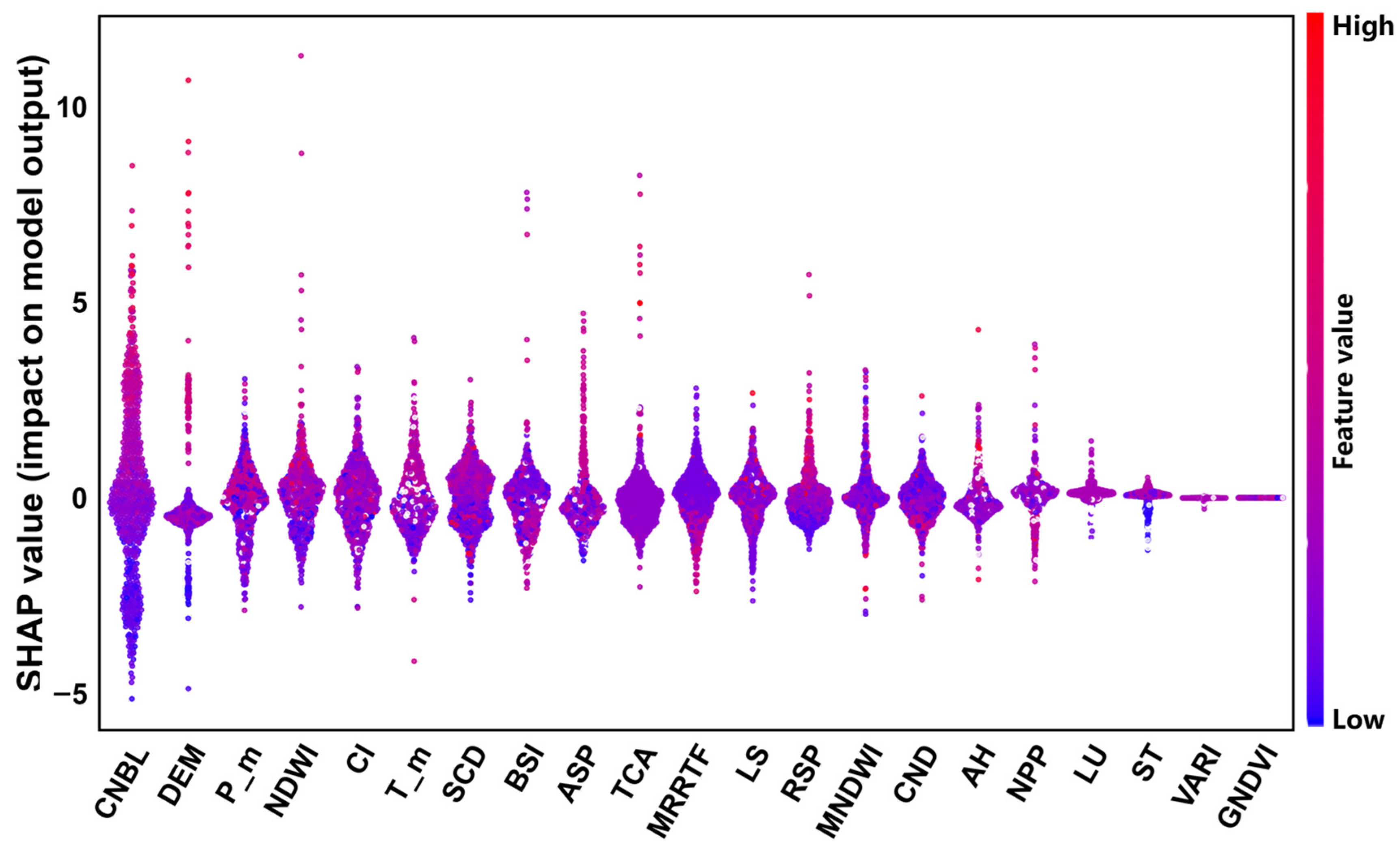
Figure 4 shows the distribution of the SHAP values for each environmental variable, with positive values indicating a positive impact on the SOM content and negative values indicating a negative impact on the SOM content. In
Figure 4, the overall importance of each variable is shown, with the x-axis representing the ranking of environmental variable importance and the y-axis representing the average SHAP value of each influencing factor.
As shown in
Figure 5, the importance of SR, VARI, GNDVI, and NDVI is relatively low, and the SHAP values are concentrated around 0. However, CNBL, which contributes 20.68% to the model, and DEM, with a contribution rate of 5.57%, are of relatively high importance. The bee colony plot in
Figure 5 shows that the CNBL and DEM have a significant impact on the SOM content. The overall importance and direction of influence of variables are shown. In
Figure 5, feature ranking (x-axis) represents the importance of the environmental variables, the SHAP value (y-axis) represents the unified index of the influence of a certain factor in the model, and red (blue) dots represent the value of environmental variables. SHAP > 0 represents a positive contribution. As the SHAP value increases, the positive effect of the factor on the SOM content is higher. SHAP < 0 represents a negative contribution, and, as the SHAP value decreases, the negative effect of the factor on SOM content is higher.
According to the results of the environmental variable driving force analysis of the soil organic matter content in the study area, terrain factors, climate factors, and biological factors are important environmental variables that affect the spatial distribution of the SOM in the study area, which is consistent with the conclusion of RF. Among them, terrain factors reflect not only the regional environment but also the influence of hydrogeological features on the distribution of soil properties. Climate factors not only directly affect the decomposition rate of soil organic matter but also indirectly affect soil organic matter content by influencing soil moisture content and vegetation type. Biological factors affect the distribution of organic matter through vegetation cover and growth conditions.
3.5. Spatial Distribution of Soil Organic Matter
The prediction accuracy of the optimization model based on the combination of RF and GA variables is relatively high, achieving an R
2 of 0.49, an MAE of 3.01 g·kg
−1, an RMSE of 3.49 g·kg
−1, and an LUCC of 0.67. The fitting with actual values indicates that the model can effectively predict the SOM content. To allow for a visual comparison of the SOM prediction results of different models, we display the prediction results of all models within the same range (
Figure 6,
Figure 7 and
Figure 8). The SOM content in the predicted graph exhibits a significant spatial variability in distribution. The prediction results indicate that, in the study area, the SOM content is higher in the northern and eastern mountainous areas, while it is lower in the central area with a flat terrain, and a few high values are also distributed in southern cities and mixed forest areas. SOM content is generally higher in mountainous regions and lower in plains. However, this spatial pattern does not necessarily indicate that terrain undulation is the primary driver of soil organic matter heterogeneity. This is because while terrain undulation can influence soil erosion and sedimentation processes, these effects are often indirect and localized. Although steeper topographies may exacerbate erosion, SOM distribution depends not only on erosion intensity but also on the stability of depositional environments. In the northern and eastern mountainous areas, the main land cover type is forest, with dense vegetation and a complex terrain; less human intervention allows vegetation to continuously input organic matter into the soil, and the mountainous terrain may slow down soil erosion, resulting in a higher accumulation rate of organic matter in the soil. The flat areas in the central region are mainly farmland, and more agricultural activities such as long-term cultivation and fertilization may accelerate the decomposition of organic matter. In addition, areas with a flat terrain are more susceptible to rainfall and wind erosion, further reducing the SOM content.
The prediction results of the three models are shown in
Figure 4. It can be seen that the SOM spatial distribution prediction results of RF and RF-GA are very similar. The difference is that the OK prediction results are very smooth, while the RF and RF-GA prediction models can highlight the spatial details and changes in the SOM, demonstrating richer SOM spatial variation information. The OK valuation significantly differs from the original data. The areas exhibiting high SOM are mainly distributed in areas with significant terrain fluctuations, which is conducive to the accumulation of SOM.
4. Discussion
4.1. Advantages of RF-GA Model
Compared to traditional Ordinary Kriging (OK) and random forest (RF) methods that rely on full-variable predictions, the RF-GA model utilized in this study offers several distinct advantages. Notably, it effectively addresses spatial heterogeneity in complex regions. Unlike traditional methods that often require the classification of land use types, the RF-GA model enhances the model’s ability to discern data features, leading to improved fitting accuracy. Specifically, in the hilly basin of Lanxi City, where the study is situated, the complex topography induces significant spatial variability. The RF-GA model excels in capturing the nonlinear relationships between soil organic matter (SOM) and environmental variables across different topographic units. For example, in hilly areas, slopes and valleys exhibit distinct hydrological and micro-climatic conditions, which the RF-GA model can accommodate, whereas traditional methods may overlook these variations.
When comparing the RF-GA model with OK and RF methods in predicting SOM in such complex regions, the RF-GA model demonstrates clear superiority. In particular, the RF-GA model is capable of effectively selecting the key environmental covariates that substantially contribute to the model’s performance. In regions with complex topography, such as our study area, variables like slope gradient and aspect play a crucial role in SOM distribution. The genetic algorithm (GA) embedded within the RF-GA model can identify these important topographic factors, thereby eliminating low-contribution variables that could otherwise interfere with model accuracy. This significantly enhances the accuracy of SOM predictions. The genetic algorithm optimizes the RF model by mimicking natural selection processes. By encoding model parameters as genes and applying operations such as selection, crossover, and mutation, the GA helps the model search for the optimal combination of parameters within a large solution space, thereby improving its predictive performance.
4.2. Explanation of Environmental Variables
The influencing factors of SOM exhibit considerable spatial variation due to both natural and anthropogenic disturbances [
33]. In the hilly basin area of Lanxi City, topographic, climatic, and biological factors are identified as key determinants of SOM, and they exhibit certain threshold or peak effects.
Topographic factors have a profound impact on SOM distribution. In this hilly region, elevation, slope gradient, and aspect are significant variables. Elevation influences temperature and precipitation patterns, which, in turn, affect the decomposition and accumulation of SOM. Higher elevations typically experience lower temperatures, which slow the decomposition rate, resulting in higher SOM content. The slope gradient influences soil erosion and deposition processes. Steeper slopes are more prone to erosion, leading to the loss of SOM-rich topsoil, while gentle slopes are more favorable for SOM accumulation. Aspect affects the amount of solar radiation received, which influences micro-climates and vegetation growth, both of which are closely related to SOM distribution. Among topographic variables, the CNBL and DEM exhibit the most substantial impact on SOM distribution, consistent with findings from related studies [
34,
35,
36]. Terrain factors regulate SOM distribution by affecting soil water content, erosion–deposition processes, vegetation distribution, and micro-climates [
8].
Climate factors also influence SOM dynamics, affecting accumulation and decomposition through temperature, precipitation, vegetation, and microbial activity. In warm and humid climates, high temperatures and abundant precipitation accelerate SOM decomposition by promoting microbial activity. Conversely, in cold and arid regions, low temperatures and limited precipitation slow down decomposition, favoring SOM accumulation.
Biological factors impact SOM distribution through vegetation growth, litter input, and biological activity [
37]. Dense vegetation cover increases litter deposition, providing a major source of SOM. Moreover, different vegetation types exhibit varying root exudation patterns, which influence soil microbial communities, thus affecting the decomposition and transformation of SOM.
4.3. Limitations and Potential Improvements
4.3.1. Insufficient Data Scale and Representativeness
This study is based on data collected from 1560 sampling points across Lanxi City. While this sample size provides valuable insights, its limited spatial distribution may affect the generalizability and robustness of the model’s predictions, especially when applied to other regions with differing environmental conditions. It is important to note that the study area is situated in a hilly basin region, where the spatial variability of soil organic matter (SOM) is inherently high due to complex topography. As a result, the prediction accuracy of SOM models in such areas is generally lower compared to flatter regions. This phenomenon is well-documented in previous studies and reflects the challenges of modeling SOM in regions with such high spatial heterogeneity. Furthermore, environmental variables, particularly climate-related factors, were considered without accounting for temporal dynamics such as seasonal or long-term fluctuations, which could influence SOM distribution. In future research, incorporating time-series data and increasing the sampling points could help mitigate these limitations, improving both the spatial and temporal representation of the data.
4.3.2. Directions for Model Optimization
Although genetic algorithms (GAs) have proven effective in enhancing the performance of the model by optimizing variable selection, it does come with high computational complexity and longer optimization times. Additionally, both the random forest (RF) and RF-GA models tend to underperform in areas with sparse extreme values, which are often associated with special geographical conditions or environmental factors. This challenge is inherent in SOM predictions for complex areas, where extreme values, typically linked to specific local factors, are underrepresented in the sample. As a result, the model may overestimate values near the global mean, reducing prediction variability. To address this issue, future research should focus on optimizing both the model and the data, incorporating techniques such as oversampling or enhanced sampling strategies for extreme values. Further, model calibration techniques, such as post-prediction adjustments or refinement of algorithmic parameters, can help correct for these biases, improving prediction accuracy in regions with sparse extreme values.
4.3.3. Applicability and Interaction Analysis of Explanatory Methods
The SHAP (Shapley Additive Explanations) interpretation method provides valuable insights into the contributions of environmental variables to SOM, enhancing the model’s explainability. However, it comes with significant computational complexity and resource demands, particularly as the number of environmental variables increases. Moreover, this study did not explore the interactions between different environmental factors, which may be crucial for a more comprehensive understanding of their combined effects on SOM distribution. In the future, we suggest incorporating a more efficient explanatory model that combines SHAP interaction values to investigate how multiple environmental factors interact and influence SOM distribution. This would allow for a more detailed, nuanced understanding of the environmental processes at play.
5. Conclusions and Prospects
This study, based on soil surveys and measured data, utilized Kriging interpolation (OK), the random forest (RF) model, the random forest model optimized with genetic algorithm variable combination (RF-GA), and the SHAP interpretation method to analyze the spatial differentiation characteristics and key influencing factors of soil organic matter (SOM) in Lanxi City, as well as their impacts. The following key conclusions were drawn:
The spatial distribution of SOM in the study area is influenced by factors such as terrain, climate, and biological factors, exhibiting clear spatial differentiation patterns. Specifically, SOM content is higher in the northern and eastern mountainous regions, while lower in the central, flat areas. Additionally, some high SOM values are observed in the southern cities and mixed forest areas. This distribution pattern indicates that SOM spatial variability is not only influenced by topographic changes but also closely related to local climate and vegetation factors.
The RF-GA model, optimized by the genetic algorithm-based variable combination, demonstrates excellent performance in extracting environmental variables. Compared to the traditional RF model, which uses full-variable prediction, the RF-GA model significantly improves the accuracy of SOM predictions. Particularly in complex regions, this model can better identify and optimize key variables, excluding the interference of low-contribution variables, thereby enhancing prediction accuracy. As such, the RF-GA model presents a reliable tool for SOM prediction in complex areas.
Further analysis using the RF-GA-SHAP model reveals that the primary factors influencing the spatial distribution of surface SOM in the hilly basin area of Lanxi City include CNBL, DEM, P_m, NDWI, CI, T_m, SCD, and BSI. These factors not only reveal the patterns of SOM spatial variation but also provide scientific evidence for soil management practices and sustainable agricultural development. Notably, the use of the SHAP method helps to quantitatively explain the specific effects of these environmental variables on SOM distribution, offering intuitive and actionable support for land use decision making.
The innovative aspect of this study lies in the combination of the RF-GA model and the SHAP method, proposing a novel SOM prediction model. In complex topographic regions, the optimization process of the genetic algorithm effectively selects important environmental variables, while the SHAP method provides quantitative explanations for their impacts on SOM distribution. This integrated approach not only improves prediction accuracy but also enhances model interpretability, offering new insights for future SOM research and environmental management.


