Assessment of Landslide Susceptibility Based on the Two-Layer Stacking Model—A Case Study of Jiacha County, China

Abstract

The challenge of obtaining landslide susceptibility zoning in Tibet is compounded by the high altitude, extensive range, and difficult exploration of the region. To address this issue, a novel evaluation approach based on Stacking ensemble machine learning is proposed. This study focuses on Jiacha County, adopts the slope unit as the evaluation unit, and picks up 14 evaluation factors that symbolize the topography and geomorphology, environmental and hydrological features, and basic geological features. These landslide conditioning factors were integrated into a total of 4660 Stacking ensemble learning models, randomly combined by 10 base-algorithms, including AdaBoost, Decision Tree (DT), Gradient Boosting Decision Tree (GBDT), k-Nearest Neighbors (kNNs), LightGBM, Multilayer Perceptron (MLP), Random Forest (RF), Ridge Regression, Support Vector Machine (SVM), and XGBoost. All models were trained, using the natural discontinuity method to classify landslide susceptibility, and the AUC value, the area under the ROC curve, was taken to evaluate the model. The results show that the maximum AUC values in the 9 models performing better reach 0.78 and 0.99 over the test set and the train set. Most of the areas identified as high susceptibility and above show consistency with the interpretation of the existing geological field data. Thus, the Stacking ensemble method is applicable to the landslide susceptibility situation in Jiacha County, Tibet, and can provide theoretical support for disaster prevention and mitigation work in the Qinghai–Tibet Plateau area.

1. Introduction

Landslide disasters are among the most significant geological disasters, posing a grave hazard to human life and property. They are challenging to detect, have a substantial impact, and result in severe consequences [1]. Jiacha County, located in the southeastern part of Tibet, is subject to the influence of several tectonic faults, including the Yarlung Zangbo River fault, the Jinsha River fault, along with the structural features of the Hengduan Mountains. This unique geography has resulted in high mountains and deep valleys with a broken surface. It poses additional challenges to disaster mitigation and response efforts [2,3,4]. Concurrently, the region is characterized by substantial daily and annual temperature variations, with a general upward trend since the 1980s. This has resulted in recurrent freezing and thawing cycles of the rock mass [5,6]. This phenomenon is a key factor in landslide disasters and the study of landslide susceptibility in this area is crucial in resolving the conflict between local engineering construction and the extreme natural environment.

Existing methods for assessing landslide susceptibility include qualitative and quantitative methods [7]. Qualitative methods principally combine geological survey data, landslide catalog data, and expert knowledge to evaluate the relevant area, which is more subjective. However, with the continuous advancement of environmental monitoring technology, the emergence of machine learning capabilities, and the development of Geographic Information System (GIS) technology, the utilization of machine learning and GIS technology to perform quantitative assessments of landslide susceptibility has become a novel research direction in the digital age. This approach offers a new high-precision objective solution for quantitative landslide susceptibility assessment at the data level [8,9,10]. Machine learning models in current use are predominantly composed of fundamental models, including Decision Tree, Support Vector Machines, Regression prediction and analysis, Random Forests, and Gradient Boosted Decision Tree [11,12,13]. Additionally, there are recently developed deep learning models tailored for the geological environment of specific regions, such as artificial neural networks and deep neural networks [14,15]. When combined with actual geological conditions, these models will provide new physical meaning to conventional data fitting methods. A new connection will be established between data and entities, so that the relevant data output by the model can represent a certain actual physical meaning in the region [16,17,18]. This development has emerged as a significant foundation for leveraging machine learning methods for quantitative landslide susceptibility mapping.

The Qinghai-Tibet Plateau region is distinguished by unique geological conditions, which have made it challenging to obtain conditioning factors. Consequently, the existing research on landslide susceptibility in this region remains incomplete. Most of the current studies have focused on the landslide susceptibility caused by the region’s unique environment and its changes. These studies include landslides caused by geological fault zones, landslides caused by the freeze–thaw cycle of the region’s permafrost, and special landslides affected by environmental conditions such as climate warming [19,20,21]. These studies employ various methods to quantify the unique characteristics of their respective constituencies and utilize selected machine learning models to conduct the susceptibility assessment. These methods have been shown to offer certain advantages in addressing the unique characteristics of their respective environments. However, it should be noted that the assessment outcomes are significantly influenced by the specific factors that have been selected for analysis. These methods are not designed to provide a comprehensive understanding of the relationship between environmental factors and landslide susceptibility. And in the machine learning prediction process, the majority of studies employ a single model for fitting and prediction, disregarding the limitations of a single model when confronted with data. This approach fails to ensure the robustness of the overall model, making it challenging to identify and enhance the model effect that has fallen into local optimum or other such challenges [22]. However, the employment of a range of conditioning factors, the consideration of specific conditions of the Qinghai–Tibet Plateau region, and the implementation of a multi-model ensemble prediction scheme can propose a viable solution to these challenges.

In this study, the concept of Stacking is used to achieve multi-model collaborative prediction, a machine learning model that combines the prediction results of multiple models, operates in both series and parallel, exhibits a certain degree of data fitting capability, and shows robust performance [23]. This model has demonstrated outstanding performance in short-term electricity consumption prediction, prostate cancer detection, and plant disease recognition [24,25,26]. Jiacha County in the Qinghai–Tibet Plateau was selected as the research area, and 10 mainstream algorithms were employed, including AdaBoost, Decision Tree (DT), Gradient Boosted Decision Tree (GBDT), k-Nearest Neighbor (kNN), LightGBM, Multilayer Perceptron (MLP), Random Forest (RF), Ridge regression (Ridge), Support Vector Machine (SVM), and XGBoost. These algorithms were utilized in various combinations to form the Stacking ensemble learning algorithm. The Tree Parson Estimator hyperparameter optimization solution was employed, with the annual average temperature serving as the region’s unique geological conditions. The known landslide locations and the environmental data of the landslide units were entered into the model for the purpose of joint training. After comparison, some algorithm combinations that demonstrate exceptional performance are going to be identified. These combinations are employed to carry out the landslide susceptibility map. This will provide effective theoretical guidance for industrial production, including local infrastructure construction and the prediction and prevention of geological disasters.

2. Region Background and Data Sources

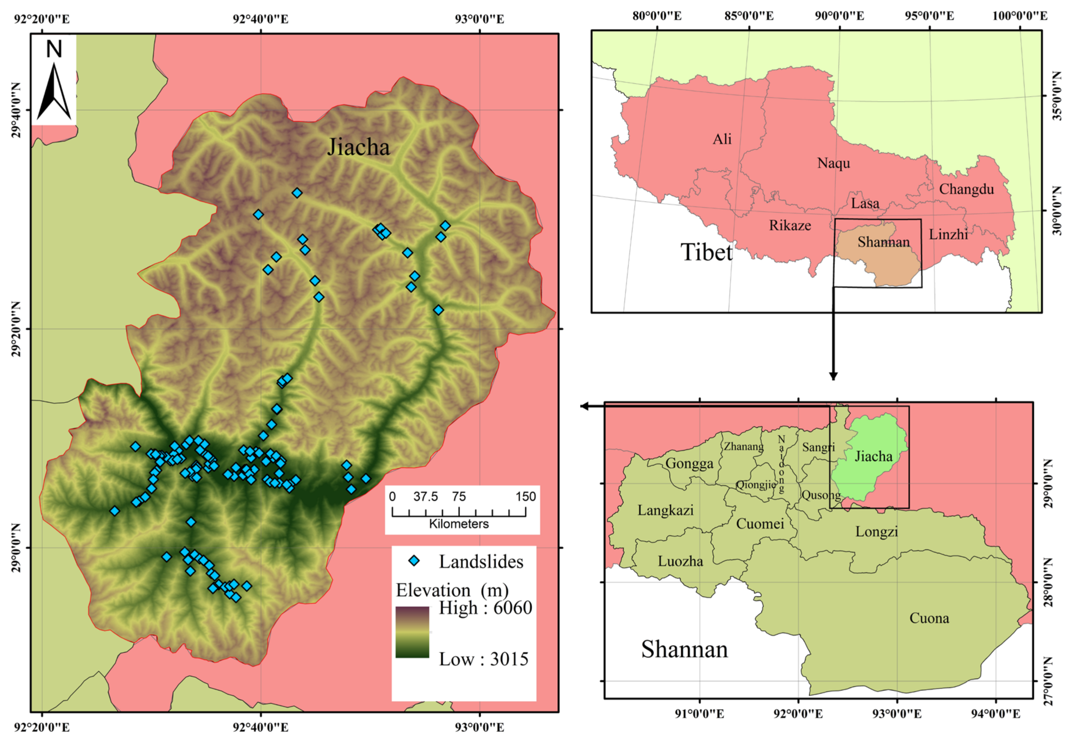
2.1. Study Area

The research area covers Jiacha County, which is characterized by its high altitude, diverse landform, including mountains and deep valleys, and significant seasonal climate variability. This region is particularly susceptible to landslides, which have the potential to significantly impact infrastructure development and the safety of individuals and property. The county is located in the southeastern part of the Tibet Autonomous Region, with geographical coordinates spanning from 92°14′E to 93°07′E and 28°49′N to 29°43′N, as shown in Figure 1. The county’s dimensions are approximately 88.2 km in width, extending from east to west, and 102.2 km in length, ranging from north to south, with a total area of approximately 4646 km². The county is situated within a highland temperate semi-arid monsoon climate zone, exhibiting an average annual precipitation of 492.7 mm.

The predominant geological characteristic of Jiacha County is a tilting trend that traverses the region from north to south, with the Yarlung Zangbo River fault zone passing through the southern part of the county. The area’s altitude ranges from 3015 to 6060 m above sea level. The area is affected by the stress caused by the unique geological structure of the surrounding fault, as well as other triggering factors such as temperature and rainfall. These factors have led to the development of geological hazards in the area, especially landslides controlled by rock fracture surfaces under long-term high stress loads.

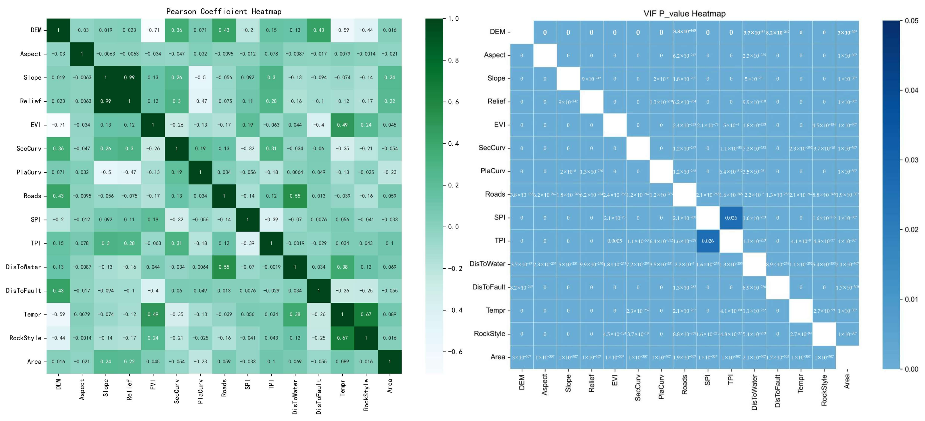
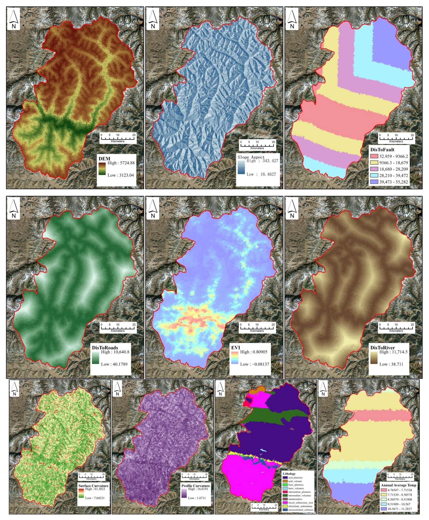
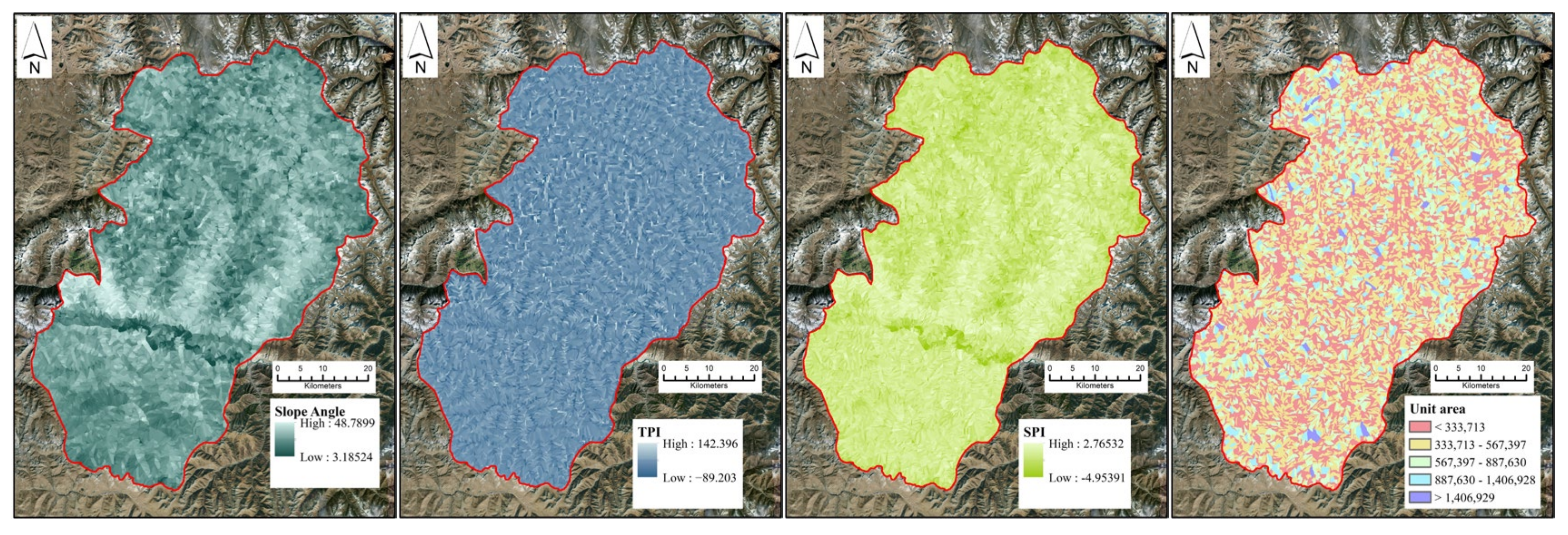
2.2. Predisposing Factors

The data selected for this study were obtained from the Chinese national public data website. The specific sources are listed in

Table 1. Sources and scales of the conditioning factors in this study.

Factor Type	Factor Name	Scale	Sources
Terrain Factor	DEM	30 m	Geospatial Data Cloud (https://www.gscloud.cn)
	Slope aspect	30 m	Generated from DEM by ArcGIS
	Slope angle	30 m	Generated from DEM by ArcGIS
	Surface relief (QFD)	30 m	Generated from DEM by ArcGIS
	Surface curvature (SecCurv)	30 m	Generated from DEM by ArcGIS
	Profile curvature (PlaCurv)	30 m	Generated from DEM by ArcGIS
	TPI	30 m	Generated from DEM by ArcGIS
Environmental and Hydrological Factor	Distance to Roads	30 m	OpenStreetMap (https://www.openstreetmap.org)
	Distance to Water	30 m	OpenStreetMap (https://www.openstreetmap.org)
	Annual average temperature	1000 m	Geospatial Data Cloud (https://www.gscloud.cn)
	EVI	250 m	Geospatial Data Cloud (https://www.gscloud.cn)
	SPI	30 m	Generated from DEM by ArcGIS
Fundamental Geological Factor	Distance to fault	30 m	OpenStreetMap (https://www.openstreetmap.org)
	Lithology (RockStyle)		1:250,000-scale Regional Geological Map
Other	Area of evaluation unit	1 m2	Generated from DEM by ArcGIS
	Landslide locations		Field survey

. The slope aspect, slope angle, surface relief, profile curvature, surface curvature, Standardized Precipitation Index (SPI), Topographic Position Index (TPI), and area of the evaluation unit were all generated from digital elevation data using the relevant tools in the ArcGIS 10.8 software.

The terrain factor includes the DEM, slope aspect, slope angle, surface relief, profile curvature, surface curvature, and TPI. The occurrence of landslides is significantly influenced by the terrain, especially by the undulating shape of the slope [27]. These factors possess the capacity to characterize the physical characteristics of the surface, and when combined, they can more accurately depict the solid surface shape of the region, thereby establishing a close correlation between the data and the actual physical feature.

In Jiacha County, the predominant landslides are shallow landslides and rock landslides. These are characterized by their relative shallowness and extensive coverage of the landscape, with a strong correlation to environmental factors. In the context of the Qinghai–Tibet Plateau, a region with low rainfall and low temperatures, shallow landslides and rock landslides are attributed primarily to the freeze–thaw cycle. This is significantly influenced by diurnal and seasonal temperature variations. Consequently, temperature is identified as a pivotal factor that requires consideration.

The environmental and hydrological factors include the distance to roads, distance to water, annual average temperature, Enhanced Vegetation Index (EVI), and Standardized Precipitation Index (SPI). The construction of roads results in the overall destruction and local reinforcement of the original rock mass, which causes the rock mass structure in the vicinity of the road to be altered and its water permeability to be affected. Water systems and vegetation fill the pores inside the rock mass. This destroys the original structure and produces cracks or new fracture surfaces. Temperature exerts a direct influence on the elasticity and plasticity of rocks. Additionally, it controls the volume of water in their pores, which has a significant impact on the strength properties of the rock mass.

The fundamental geological factors include the distance to fault and surface lithology. Faults are a typical structural manifestation of crustal movement, and the rock debris and cracks formed during their occurrence promote landslides. Surface lithology is an essential component of the rock constitutive relationship. It plays a pivotal role in determining the structural stability of rock masses and is also a significant factor in the occurrence of landslides. The accurate and appropriate classification and data mapping of surface lithology facilitate the abstraction of rock mass characteristics, which is conducive to further quantitative evaluation.

These features have been demonstrated to exert a certain degree of influence on the damage incurred by the rock mass during a landslide event. When employed as an input data source for machine learning algorithms, these features can accurately represent the physical characteristics of the rock mass, establishing a tangible link between machine learning and the complex dynamics of landslides. However, it should be noted that not all data are suitable for machine learning, and certain trade-offs are required.

For the 15 types of data represented in Table 1, a series of statistical analyses were conducted. These included both Pearson’s correlation coefficient and a measure of multiple collinearity. The outcomes of these analyses are illustrated in the heatmap representation displayed in Figure 2. It can be seen that the Pearson’s correlation coefficient between the slope angle and surface relief attains 0.99, signifying a remarkably high correlation among these two factors. And no abnormality was found in the collinearity analysis, due to the fact that slope has a considerable impact on the occurrence of landslides within a given slope unit. After excluding the abnormal factor of surface relief, 14 remaining factors were utilized as Jiacha County landslide conditioning factors, as shown in Figure 3.

In order to further analyze the relationship between the distribution of landslide disasters and the entire region from a data perspective, the proportion of landslide conditioning factors in landslide points and the Jiacha County are analyzed, as shown in Figure 4. The analysis indicates that the majority of conditioning factors exhibit discrepancies in their distribution between landslide points and the entire dataset. For instance, in the entire region, which has an altitude of 4335 m or higher, landslide disasters are predominantly concentrated below 3830 m. The distribution of the entire region from roads, faults, and rivers is relatively uniform, while landslide disasters are predominantly concentrated in closer proximity to these features. Furthermore, landslide points are more prevalent in areas exhibiting low EVI values and sediment lithology. The observed variations can be attributed to the fact that landslides are predominantly concentrated in proximity to rivers and roads, as well as the significant influence of tectonic activity and river undercutting. The Yarlung Zangbo River Valley exhibits the highest concentration of landslides. The development center of Jiacha County is distributed along the rivers, due to the convenience of transportation and the utilization of water resources. Human engineering activities, including the construction of infrastructure and the disruption of vegetation, can further contribute to landslide occurrence. Consequently, the landslide disaster points are distinct from the overall situation in the entire region, with respect to these indicators.

A total of 124 landslide points were collected in the study area. After field investigation, it was found that the area within 2000 m of the landslide site can be regarded as the landslide risk area, and the area within 4000 m can be regarded as the buffer zone, which can meet the area characteristics of most of the investigated landslide points. And the landslide occurrence area was delineated as the slope units within a radius of 2000 m, centered on each landslide point, and signed their landslide state value as 1. The landslide buffer area was delineated as the slope units within a radius of 2000 m to 4000 m, centered on the landslide point. The landslide state value was set to 0 in this case, and the remaining area was left blank. The abovementioned operation yielded a total of 5083 slope units with indicated landslide status, including 2100 in the occurrence area and 2983 in the buffer area. Combining the corresponding landslide conditioning factors with the landslide status value, the landslide dataset of Jiacha County was established, partitioning according to the percent of 80% and 20% for the training set and test set. All data will be 0–1 normalized before being used for machine learning training.

2.3. Division of Evaluation Units

In regions exhibiting variations, it is imperative to implement distinct evaluation unit division schemes, taking into account geological conditions, natural environments, data precision, and other reginal characteristics. The prevailing methodologies for this purpose are the grid cell method and the slope unit method. Grid cell prediction accuracy depends on the grid size selected and is generally high. The grid cell method is particularly well suited for situations where geological conditions are clearly defined and data quality is enough. In contrast, the slope unit method offers slightly lower predictive precision, influenced by the dimensions of the delineated slope units. The slope unit method is particularly well suited for scenarios where the DEM is clearly defined and the precision of the remaining data tends to be lower.

Due to the data precision limitations of the above sources and the partial lacking of surface temperature and EVI data, this study employs the improved slope unit method to divide the evaluation units in ArcGIS software [28], and manually corrects abnormal slope units based on the natural conditions of landslide development to ensure the predictive precision based on the selection of the slope unit method for splitting evaluation units. A total of 12,868 units were divided, with an average area of 341,033 m². The corresponding data within each slope unit takes the average of the raster data covered by the slope unit. The surface lithology is calculated based on the most dominant lithology of the recorded data within the landslide unit, and the missing data in the original dataset are estimated based on the nearest raster data.

3. Methodology

3.1. Hyperparameter Optimization and Base Model

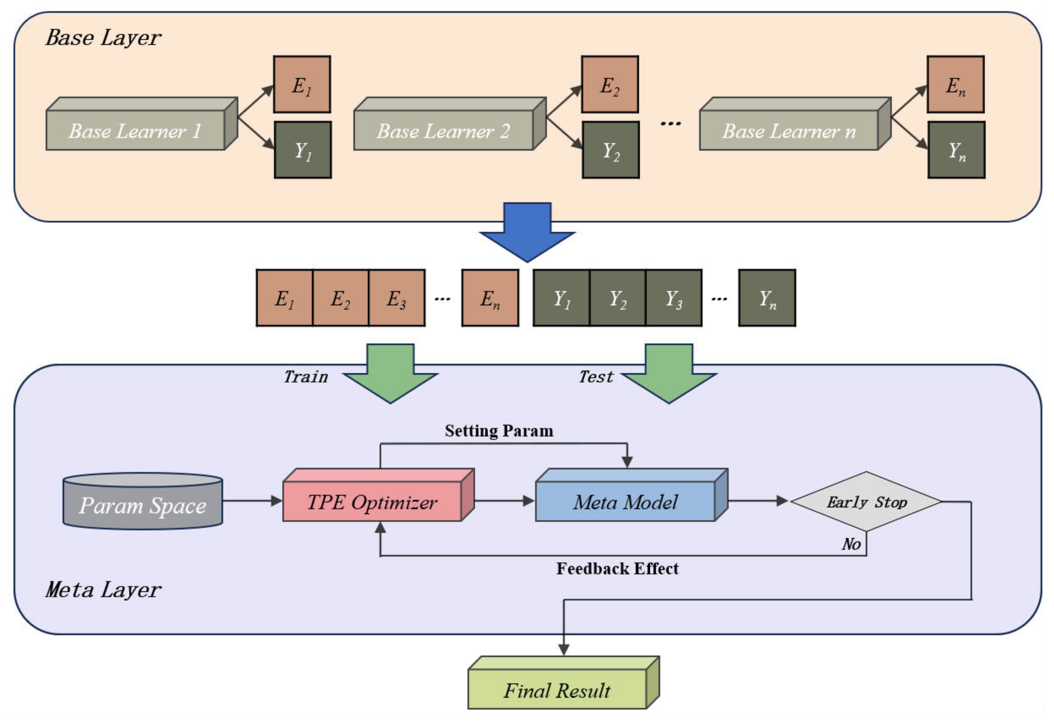
The selection of the base model is a critical component of the Stacking method. The prediction results of the base model directly affect the predictive precision of the ensemble model. The combination of appropriate base models has been shown to enhance the predictive precision of the overall model. In this study, a total of 10 algorithms shown in Figure 5 were selected to establish the pool for the base model. These included the tree structure algorithms Decision Tree (DT), Gradient Boosted Decision Tree (GBDT), Random Forest (RF), LightGBM, AdaBoost, and Extreme Gradient Boosting (XGBoost); the pattern recognition algorithm k-Nearest Neighbor (kNN); the biased weighted algorithm Ridge Regression (Ridge); the vector machine algorithm Support Vector Machine (SVM); and the neural network algorithm Multilayer Perceptron (MLP). The model pool serves as the foundational framework, with each algorithm undergoing optimization through the Tree Parzen Estimator (TPE) optimization method.

The TPE solution is an efficient Bayesian parameter optimization algorithm. It organizes a tree structure to define a mean-centered Gaussian distribution index for model parameters and mean deviation. This solution employs an iterative feedback mechanism to optimize hyperparameters in iterative tests. This process is intended to rapidly maximize the expected improvement within a limited number of iterations [29]. This study employs the TPE solution to ensure the quality of the basic model parameters within certain time constraints, improve the predictive ability of the ensemble model, and enhance the credibility of the model results.

The Decision Tree (DT) is a fundamental algorithmic structure that utilizes a combination of nodes and directed edges. Initiating from the root node, it systematically compares the feature nodes within the tree and identifies the optimal attribute for classification. This process ensures that the categories contained by the tree’s branch nodes are as similar as possible, thereby culminating in the successful completion of the classification process [30].

The Gradient Boosting Decision Tree (GBDT) employs a combination of classification and regression trees as weak learners, iteratively minimizing their loss function. This algorithm has been shown to demonstrate effective management of high-dimensional data, possess certain convergence properties, ensure local and global optimization advantages, address issues of overfitting and underfitting, and enhance classification performance [31].

Random Forest (RF) is an ensemble learning algorithm that combines multiple Decision Trees to achieve classification using the bagging strategy during the training and testing stages. The RF algorithm demonstrated a gradual convergence during iterations, despite significant fluctuations in the initial fitting [32]. This suggests that the model possesses practical enhanced predictive capabilities.

The LightGBM algorithm is based on Decision Trees, utilizing the specific characteristics of the data to construct a corresponding histogram and discretize the data. Subsequently, histogram analysis is utilized in order to calculate the optimal split gain. Nodes are selected at varying depths to complete the split, ensuring that the data can be classified with enhanced precision in as few iterations as possible [33].

The AdaBoost algorithm is a tree-structured model for structured learning. It adjusts the sample weight according to the prediction results of each cycle, focusing on difficult samples with higher weights. The algorithm ultimately reduces the training error cyclically by decomposing these challenging instances into a single conclusive hypothesis, thus achieving accurate prediction on the dataset [34].

Extreme Gradient Boosting (XGBoost) is an ensemble learning algorithm based on the gradient boosting strategy. It iterates freely based on parameters and training data, introduced the second derivative as the loss function, and is assisted by multiple means to further enhance the fitting effect [35].

The k-Nearest Neighbor (kNN) algorithm is a statistically mature pattern recognition algorithm that plays a major role in machine learning. The algorithm is designed to estimate the category of a sample by leveraging the majority of the k-Nearest Neighbor samples in the feature space. This estimation is made through a voting method determined by the distance of the sample to the kNN samples. The algorithm then applied this estimation to make a classification decision.

Ridge regression is a regularization method for linear regression that offers certain advantages when dealing with data that exhibit significant multicollinearity. It is capable of making multiple predictions in the presence of different features, assigning biased weights to features and emphasizing the contribution of the primary features to the prediction results [36], leading to a certain degree of improvement in model overall performance.

Support Vector Classification (SVC) is a foundational algorithm that utilizes a support vector machine to categorize samples by employing a corresponding kernel function, offering a certain flexibility. The kernels most frequently employed include linear, polynomial, and Gaussian. Linear kernels, which can be regarded as a special case of Gaussian kernels, possess strong capabilities for generalization.

Multilayer Perceptron (MLP) is a specific type of artificial neural network. It is an algorithmic model that abstractly simulates biological neural networks. The architecture of the MLP comprises an input layer, an output layer, and multiple hidden layers [30]. Due to its ability to capture complex interactions between input data, its strong representational capacity, and its reliability in dealing with non-linear problems and high-dimensional data, the MLP has become a typical solution in many fields of study.

3.2. Stacking

The concept of Stacking ensemble learning involves the application of the prediction outcomes from a collection of machine learning algorithms as input, with suitable algorithms from the subsequent group, referred to as the meta layer, being used. These reused algorithms are then utilized to refit and predict based on the results generated by the initial group. In essence, a parallel training process occurs at the base layer, while the algorithms in the meta layer are serially integrated to combine the heterogeneous model’s prediction outcomes. This concept has the potential to enhance the precision of prediction outcomes and consolidate the training and prediction patterns exhibited by individual basic models. This enhancement in performance is particularly evident in scenarios where the initial group of basic models displays substantial disparities [37], resulting in a more pronounced improvement in the overall model performance.

However, directly employing the training set data for the training of the base layer model and the outputting for the meta layer input data will result in the repeated application of the training set data. This repetitive use is susceptible to overfitting in the base layer. Subsequent to the re-fitting of the meta layer model, the performance of the overall model will be adversely affected. In order to obtain reasonably reliable training and prediction data for the meta layer of the Stacking model, the base model is typically employed to obtain the prediction results on the entire training set by using cross-validation. That is a process of dividing the original training data into K parts, taking only one part as the verification each time, and using the remaining K−1 parts as the input of the current training set of the base model. This step is repeated to obtain entire prediction data.

This study leverages 5-fold cross-validation to process each base model. The specific process is illustrated in Figure 6. Initially, the training set data are loaded, and the TPE hyperparameter optimization algorithm is performed on the base model with the parameter space that is pre-determined. This process yields the hyperparameters for the current model and establishes the base learner. Subsequently, the training set data are divided into five folds, K₁, K₂, K₃, K₄, and K₅, then the base learner is trained using inputs K₂, K₃, K₄, K₅, and K₁, and T is verified to obtain P₁ and T₁. These operations are repeated to obtain the current base model training set result matrix E(P₁, P₂, P₃, P₄, P₅) and the five test set results T₁, T₂, T₃, T₄, and T₅. The mean of the test set result is calculated to obtain the test set result Y(T_a).

Then, the selected base model is trained in parallel according to the stacking workflow shown in Figure 7 to obtain the corresponding validation results E₁, E₂, E₃, …, E_n and prediction results Y₁, Y₂, Y₃, …, Y_n. The validation and prediction results are then spliced separately and transmitted to the meta layer for further training, deriving the ultimate prediction results for the test set.

This study will randomly select 3 to 9 basic algorithms from the constructed model pool as the base layer. It also selects a basic algorithm randomly as the meta layer. And the parameter of each basic model will be optimized with the Tree Parzen Estimator solution. In this way, a total of 4660 Stacking ensemble models have been established, and the prediction results will be compared to identify a model combination that provides superior results and to complete the prediction of landslide susceptibility.

4. Results

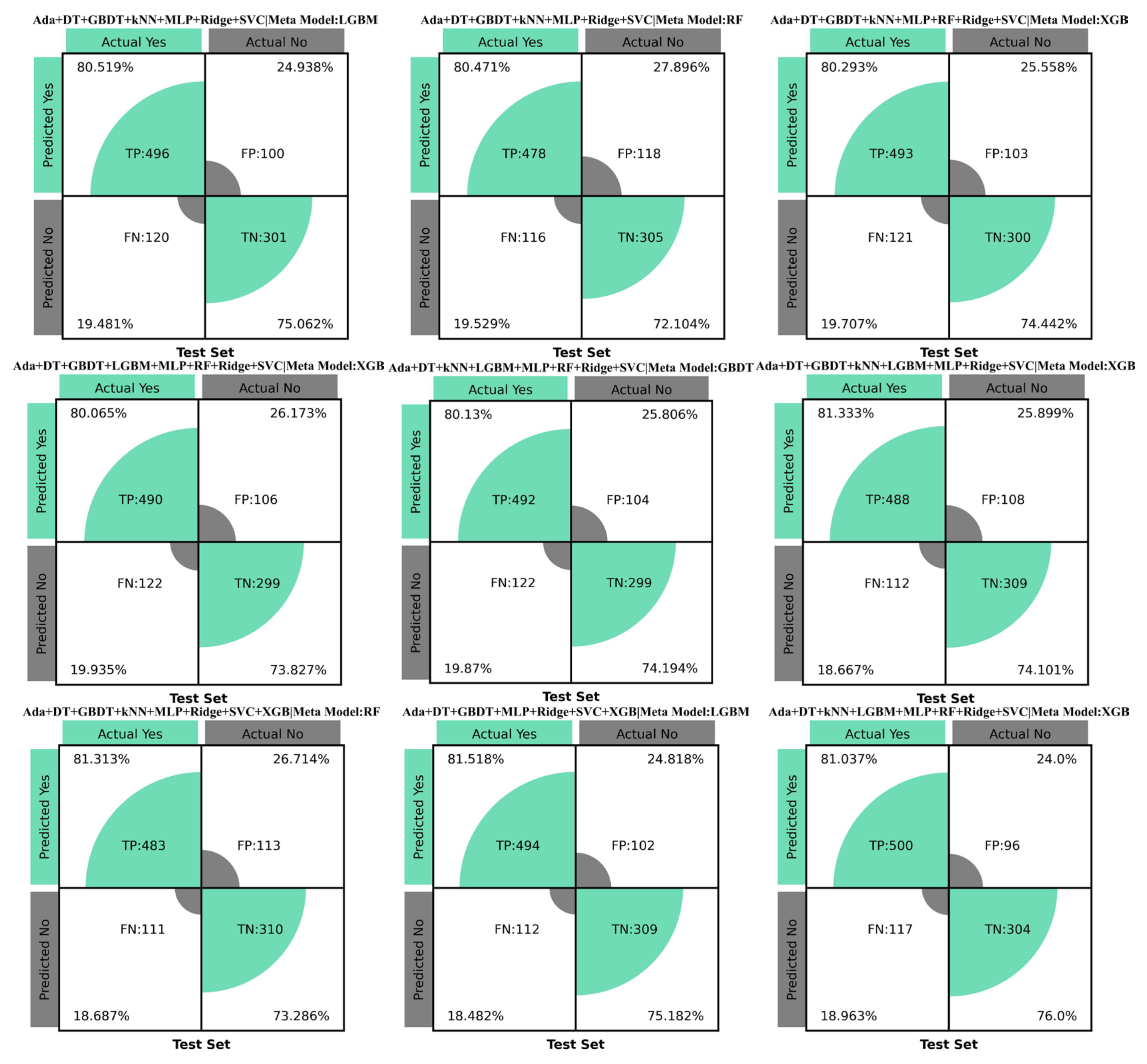
4.1. Confusion Matrix Evaluation

The confusion matrix is a method that is frequently utilized for the evaluation of classifiers. It contains four primary indicators that indicate the classification effect of the classifier: TP, FP, FN, TN, which represent true positive, false positive, false negative, and true negative. These values correspond to the four situations of the true value being correct and the predicted value being correct, the true value being incorrect but the predicted value being incorrect, the true value being correct but the predicted value being incorrect, and the true value being incorrect and the predicted value being correct. These four indicators offer a visual representation of the model’s capacity for precise prediction and directly reflect the corresponding relationship between the model’s predicted value and the actual value.

As illustrated in Figure 8 and Figure 9, the confusion matrices of the test set and training set data were constructed based on the predictions of the models that performed well in this study. The primary basis for this selection was the AUC value, with the F-score serving as a supplementary criterion. The green sectors in the matrices represent predictions that differ from the expected data. It is evident that the performance of these nine models, on the training set and the test set, has been identified as excellent. The average success rate on the test set is above 75%, which is regarded as a satisfactory prediction result.

4.2. Static Derivation Indicator Evaluation

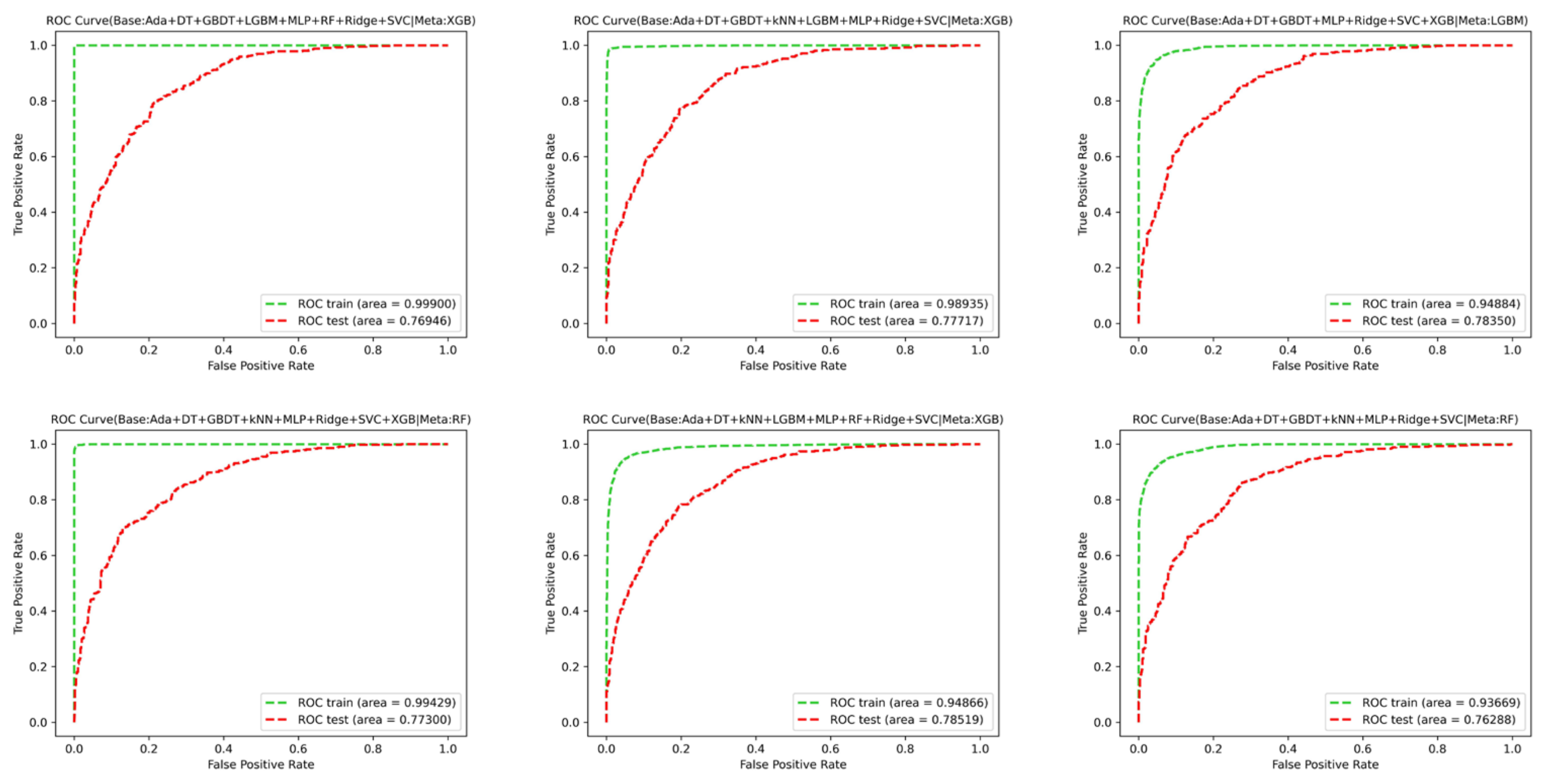
The confusion matrix offers several advantages, including its intuitive nature, clarity, and the ability to demonstrate data relationships. However, it should be noted that the number of classified elements is not sufficient to fully assess the classification effect of the model. Relying exclusively on the confusion matrix for model evaluation constitutes a one-sided approach, and quantitative assessment using its derived indicators is also necessary. Therefore, this study incorporates additional derived indicators from the confusion matrix, including accuracy, recall, precision, and the tertiary-derived indicator F-score, to provide a more comprehensive evaluation of the model’s performance.

The formula for calculating accuracy is shown in Equation (1). As is illustrated by the formula, accuracy is calculated using true positives and true negatives as the numerator and the sample population as the denominator. This calculation serves as a proportional indicator, quantifying the proportion of correctly predicted cases in data prediction. The proportion of correctly predicted cases in the sample data is directly associated with an increase in accuracy.

$$Accuracy={\displaystyle \frac{TP+TN}{TP+TN+FP+FN}}$$

(1)

Recall, also known as sensitivity or the true positive rate, is calculated using Equation (2). This metric is designed to evaluate the proportion of true positive predictions among the actual positive examples in the sample. It serves to assess the accuracy of the positive examples in the actual prediction.

$$Recall={\displaystyle \frac{TP}{TP+FN}}$$

(2)

The calculation of precision is illustrated in Equation (3). This is another secondary derivative index of the confusion matrix. It emphasizes the proportion of true positives in the prediction results to all positive predictions, and is expressed as a percentage. This index quantifies the probability that a model will accurately predict positive results during the prediction process.

$$Precision={\displaystyle \frac{TP}{TP+FP}}$$

(3)

The F-score is a tertiary derivative index of the confusion matrix, and its calculation formula is shown in Equation (4). The F-score is a comprehensive index based on the secondary derivative index of the confusion matrix. It combines the effects of precision and recall, focusing them in one and amplifying the degree of impact on true positive cases, which is significant in imbalanced datasets.

$$F1\text{-}Score=2\times {\displaystyle \frac{Precision \times Recall}{Precision+Recall}}$$

(4)

The previously mentioned index verification was conducted on the 9 models with superior performance, and the verification results on the test set are shown in

Table 2. Static validation of confusion matrix on 9 outstanding model test sets.

Index	Accuracy	Recall	Precision	F1-Score
Model1	0.769912	0.724466	0.802013	0.7227488
Model2	0.783677	0.714964	0.832215	0.7323601
Model3	0.779744	0.712589	0.827181	0.7281553
Model4	0.777778	0.710214	0.825503	0.7257282
Model5	0.775811	0.710214	0.822148	0.7239709
Model6	0.783677	0.733967	0.818792	0.7374702
Model7	0.789577	0.733967	0.828859	0.7427885
Model8	0.779744	0.736342	0.810403	0.7345972
Model9	0.790560	0.722090	0.838926	0.7405603
Naïve Bayes	0.714847	0.631828	0.663341	0.647201
Logis Reg.	0.733529	0.610451	0.706043	0.654777
SVM	0.752212	0.627791	0.712676	0.667546

Notes: Model1 is Ada+DT+GBDT+kNN+MLP+Ridge+SVC|Meta Model:RF; Model2 is Ada+DT+GBDT+kNN+MLP+Ridge+SVC|Meta Model:LGBM; Model3 is Ada+DT+GBDT+kNN+MLP+RF+Ridge+SVC|Meta Model:XGB; Model4 is Ada+DT+kNN+LGBM+MLP+RF+Ridge+SVC|Meta Model:GBDT; Model5 is Ada+DT+GBDT+LGBM+MLP+RF+Ridge+SVC|Meta Model:XGB; Model6 is Ada+DT+GBDT+kNN+LGBM+MLP+Ridge+SVC|Meta Model:XGB; Model7 is Ada+DT+GBDT+MLP+Ridge+SVC+XGB|Meta Model:LGBM; Model8 is Ada+DT+GBDT+kNN+MLP+Ridge+SVC+XGB|Meta Model:RF; Model9 is Ada+DT+kNN+LGBM+MLP+RF+Ridge+SVC|Meta Model:XGB.

and those on the training set are shown in

Table 3. Static validation of confusion matrix on 9 outstanding model train sets.

Index	Accuracy	Recall	Precision	F1-Score
Model1	0.938225	0.921905	0.949715	0.9249881
Model2	0.96026	0.948095	0.968823	0.9517208
Model3	0.939996	0.918095	0.955414	0.9267003
Model4	0.926421	0.89381	0.949380	0.9093992
Model5	0.99882	0.997143	0.999990	0.9985694
Model6	0.988983	0.981905	0.993966	0.9866029
Model7	0.948849	0.92619	0.964801	0.9373494
Model8	0.994295	0.991905	0.995977	0.993087
Model9	0.949636	0.934286	0.960443	0.938756
Naïve Bayes	0.713969	0.656343	0.652843	0.654588
Logis Reg.	0.741023	0.632519	0.708945	0.668555
SVM	0.737825	0.624042	0.712172	0.665201

Notes: Model1 is Ada+DT+GBDT+kNN+MLP+Ridge+SVC|Meta Model:RF; Model2 is Ada+DT+GBDT+kNN+MLP+Ridge+SVC|Meta Model:LGBM; Model3 is Ada+DT+GBDT+kNN+MLP+RF+Ridge+SVC|Meta Model:XGB; Model4 is Ada+DT+kNN+LGBM+MLP+RF+Ridge+SVC|Meta Model:GBDT; Model5 is Ada+DT+GBDT+LGBM+MLP+RF+Ridge+SVC|Meta Model:XGB; Model6 is Ada+DT+GBDT+kNN+LGBM+MLP+Ridge+SVC|Meta Model:XGB; Model7 is Ada+DT+GBDT+MLP+Ridge+SVC+XGB|Meta Model:LGBM; Model8 is Ada+DT+GBDT+kNN+MLP+Ridge+SVC+XGB|Meta Model:RF; Model9 is Ada+DT+kNN+LGBM+MLP+RF+Ridge+SVC|Meta Model:XGB.

. As illustrated by the validation data presented in the tables, all 9 models displayed a certain degree of accuracy, with values 0.789 on the test set and 0.998 on the training set. The models exhibited noteworthy outcomes with regard to recall, precision, and F-score, with the F-score attaining a maximum of 0.742 on the test set and 0.998 on the training set. This finding indicates that the study possesses satisfactory hit capabilities in the static metric test, and the predicted results possess a high degree of credibility under the selected metrics.

In order to assess the performance of these nine models, a comparison was made between three benchmark models commonly employed in landslide susceptibility assessment: simple Logistic Regression, naïve Bayes, and SVM. This comparison was made both on the training set and the test set. The results indicated that the performance of the three models after TPE optimization is very similar. And in some cases, the validation result on the training set was even weaker than the result on the training set. This finding indicates that the benchmark models are not sufficiently complex to adequately handle the dataset, suggesting the necessity for enhancing their performance through model improvement.

The 9 models with superior performance in comparison to the selected benchmark model on both the training set and the test set, accompanied by a considerable drop in the error rate, substantiate the hypothesis that the Two-Layer Stacking model employed in this study possesses a more advanced level of complexity than the benchmark model. This model demonstrates enhanced capacity for fitting and prediction performance when dealing with the dataset of Jiacha County. The results also provide objective evidence, supporting the feasibility and necessity of integrating models in this study.

4.3. ROC Evaluation

The receiver operating characteristic (ROC) curve is a widely utilized method for evaluating the performance of binary classification models, with the false positive rate designated as the abscissa and the true positive rate designed as the ordinate [38]. The ROC curve and its area under the curve (AUC value) were employed to verify the prediction results obtained from each of the previous models. The ROC curve, as a dynamic evaluation technique, enables the determination of the classifier’s performance by its geometric features. The ROC curve serves as a crucial instrument for evaluating the performance of a model, with a higher upward curve corresponding to better classification accuracy and increased model credibility. As demonstrated in Figure 10, the classification performance of these 9 models is notably superior and possesses a degree of credibility.

The AUC values of the 9 models on the test set are all higher than 0.75, which can be considered as a certain processing ability when faced with unknown data for binary classification. The AUC values on the training set are all higher than 0.9, and the AUC values of four models on the training set are higher than 0.95; two of them are higher than 0.99. On the test set, the AUC value of two models reached 0.78, which means that the model has certain advantages in fitting, learning, and prediction on the training set. This shows that the selected algorithm combination has a very significant learning effect in the Stacking ensemble learning model, and also has the ability to predict unknown data, which means it is proved that the performance of the 9 algorithm combinations on the dataset is better in terms of data fitting, and they are suitable for susceptibility evaluation.

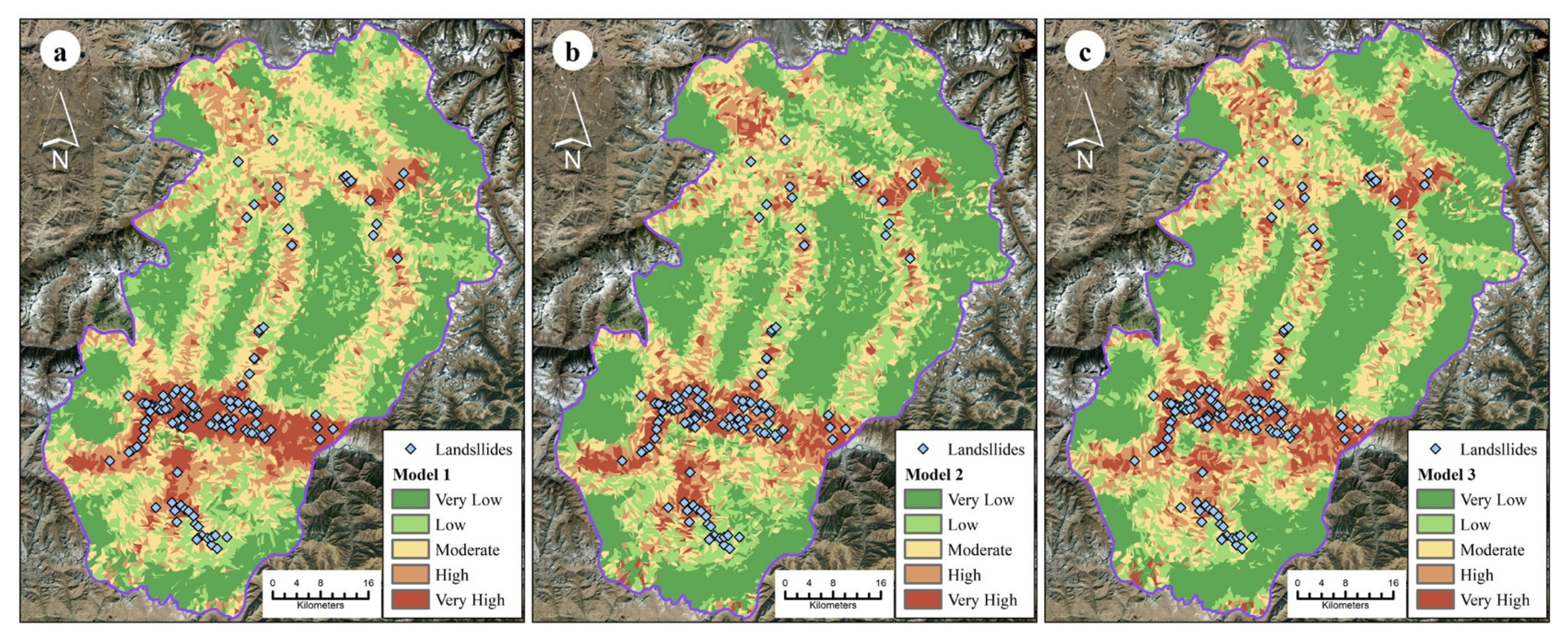
4.4. Landslide Susceptibility Mapping

This study adopts the natural breakpoint method to categorize the landslide susceptibility of the machine learning predictions within the Jiacha County. The natural breakpoint method is a grouping technique based on the idea of clustering. This method utilizes statistically significant breaks or turning points between series to analyze the boundary conditions of each category, ensuring that similar data within a group and dissimilar data between groups are appropriately classified [39]. This grading scheme has been extensively applied in various fields, including research on urban and rural construction, ecological resource evaluation, and the assessment of landslide susceptibility.

The Stacking ensemble learning model was reconstructed using the nine previously mentioned combination of algorithms. The prediction of unknown landslide state data was obtained by training with the complete landslide point dataset. This is the prediction result of the landslide susceptibility of Jiacha County in Tibet. The prediction results were then imported into ArcGIS software, where landslide susceptibility was categorized into five levels (very high susceptibility, high susceptibility, moderate susceptibility, low susceptibility, very low susceptibility) using the natural breakpoint method. This resulted in the landslide susceptibility evaluation map shown in Figure 11.

The findings indicate that the mean landslide susceptibility evaluation map obtained by means of nine different algorithm combinations encompass very low susceptibility zones, which occupy 33.96% of the total study area, amounting to approximately 1577.6 km²; and low susceptibility areas, constituting 22.97% of the total area, encompassing around 1067.2 km². The moderate susceptibility area encompasses 20.77% of the total area of the study area, equivalent to approximately 964.9 km². The high susceptibility area constitutes 14.1% of the total area of the study area, amounting to about 652.9 km². The very high susceptibility area covers 8.2% of the total area of the study area, reaching approximately 383.4 km². It is noteworthy that more than 90% of the landslide points in the study area fall into the moderate susceptibility and above areas in the nine models. Additionally, an increase in landslide point density corresponds to a significant upward trend in landslide susceptibility.

5. Discussion

In order to verify the accuracy of the machine learning model evaluation, detailed field geological surveys and analyses were conducted in areas with obvious landslide characteristics, notable geographical features of the landslide, and a strong dependence of the landslide on the environment. The applicability of the model evaluation results was validated with these areas. The prediction results of the 9 superior models were compared with the actual occurrence of landslides in two typical cases: the No.1 Hydropower Station Landslide and the Reduicun Landslide (as shown in Figure 12). The further assessment of the model evaluation results is based on this comparison.

The No.1 Hydropower Station Landslide is located on the right side of the hydropower reservoir, near the Jiacha Hydropower Station (Figure 13). The front edge of the landslide is significantly influenced by the water level of the hydropower station reservoir and seasonal temperature variations. The front edge of the landslide displays a gradual development of tensile cracks, and the phenomenon of road subsidence is evident, providing favorable potential conditions for landslide development. The landslide’s location is delineated in the slope unit, as indicated by the center point of the blue diamond in Figure 13. Among the 9 superior models, all of them mark that slope unit as very high susceptibility. Combined image and field validation has revealed that the rock in this slope unit has already cracked, and the landslide has a distinct development outline. Consequently, the slope unit should be designated as a high susceptibility zone or above. All models demonstrated a high degree of accuracy and were consistent with the observed landslide occurrence. These 9 models demonstrated a satisfactory performance in the field validation of this landslide.

The Reduicun Landslide is located on the western side of Reduicun within the urban area of Jiacha Town (Figure 14). The landslide is primarily triggered by the damage to the rocks resulting from rainfall and its own creep, in association with the long-term freeze–thaw cycles caused by the difference between day and night temperatures. Additionally, the dynamics of landslides in the region are influenced by the activity of the Yarlung Zangbo River fault, a tectonic structure that traverses the area. This landslide has previously been recorded as a disaster. The landslide is located in the slope unit, as indicated by the center of the blue diamond in Figure 14 within the landslide susceptibility mapping. Among the models evaluated, 7 models classified the slope unit as very high susceptibility, 1 model classified it as high susceptibility, and 1 model classified it as moderate susceptibility. The occurrence of specific landslide events in this area supports the prediction of its susceptibility to landslides as high or very high. A total of eight models correctly predicted this susceptibility, which is consistent with the actual situation and has applicability in the field.

Following an exhaustive examination that included a review of the confusion matrix and its associated indicators through static validation, dynamic validation of the ROC curve and its area under the curve, and field validation of the landslides using the No.1 Hydropower Station Landslide and the Reduicun Landslide, it can be concluded that the Stacking model proposed in this study can provide results that are more comprehensive and objective. This conclusion is substantiated by the model’s capacity to predict landslide susceptibility with enhanced precision, a feature attributable to a reasonable integration of the fundamental algorithm, a balanced combination, parameter optimization, and a multifaceted screening process. Moreover, the model has demonstrated notable efficacy in data fitting, unknown prediction, and field analysis. It provides specific regional insights into the occurrence and progression of landslide events at the geographical information level, and it has certain application significance and reference value.

However, during the model verification process, it was found that while most of the models with excellent performance in the data fitting stage were also effective in field verification, some of the models were not well suited for field validation support. For instance, as illustrated in Figure 14, Model 7, which has been confirmed to have occurred in a landslide event, is still designated as a medium susceptibility unit by the model. This indicates that the model exhibits a degree of negligence in establishing a connection between the data and the facts sometimes, and that the actual susceptibility level needs to be assessed by combining the prediction results of multiple excellent models. Relying on the only prediction results of a single model can lead to the trap of applicability of the model’s effects and the particularity of the selected area, which can adversely affect the accuracy of the prediction results.

From the perspective of considering the combination of multiple excellent models, this method demonstrates superior predictive performance in the unique geological and environmental of Jiacha County. It can offer a reference point for landslide susceptibility prediction in regions with similar geological and environmental conditions, such as the Qinghai–Tibet Plateau. The model’s proven complexity may also be advantageous in areas with other unique conditions, but the occasional inaccuracies in predictions within specific areas cannot be discounted.

Sections of occurrence, transportation, and accumulation of landslides possess distinct topographic characteristics, which can result in varied levels of prediction complexity. The effects of different landslide types and stages on prediction by the ensemble model can be different. The performance of the integrated prediction can be improved by separating these areas and finding suitable ensemble learning model predictions individually. This may be an important point to note when improving the performance of this model when transferring to different areas.

6. Conclusions

This study focuses on the Jiacha County, Shannan, Tibet, as the designated study area, dividing the area using an improving method of slope unit division. Fourteen conditioning factors are considered as an input dataset, including the DEM, slope aspect, slope angle, profile curvature, surface curvature, topographic position index, distance to roads, distance to water, annual average temperature, Enhanced Vegetation Index, Standardized Precipitation Index, distance to fault, lithology, and slope unit area. A total of ten algorithms are utilized in this process. These include the Decision Tree (DT), Gradient Boosted Decision Tree (GBDT), Random Forest (RF), LightGBM, AdaBoost, Extreme Gradient Boosted Tree (XGBoost), k-Nearest Neighbor algorithm (kNN), Ridge Regression, Support Vector Classification (SVC), and Multilayer Perceptron (MLP). The utilization of these algorithms enables the construction of a comprehensive total of 4660 machine learning models, leveraging the Stacking ensemble method with TPE hyperparameter optimization to perform the landslide susceptibility evaluation. The results show the following:

• In Jiacha County, high susceptibility and very high susceptibility areas account for 14.1% and 8.2% of the total area of the study area. These areas are primarily located in regions characterized by significant topographic relief, complex geological structures, and relative low altitudes, such as the Yarlung Zangbo River and its derivative rivers. In contrast, moderate and less susceptibility areas are predominantly situated in high-altitude regions across most models. These areas are distinguished by their remote locations, sparse populations, and distinctive geological structures, which to a certain extent, mitigate the risk of landslide disasters.
• The application of disparate numbers of algorithms, encompassing different types, within the two-layer structure of the Stacking ensemble method, results in a total of 4660 model combinations. These models exhibit variability in performance at the data level. Consequently, these various combinations generate disparate predicted values and evaluation results. The efficacy of models derived from multiple sources performs at an optimal level. Among the 9 models identified as excellent in this study, the static test index demonstrates an accuracy of up to 0.998 and 0.789 on the training set and test set. The area under the ROC curve for the dynamic test index reaches 0.99 and 0.78 on the training set and test set, indicating that these models possess superior data fitting and prediction capabilities.
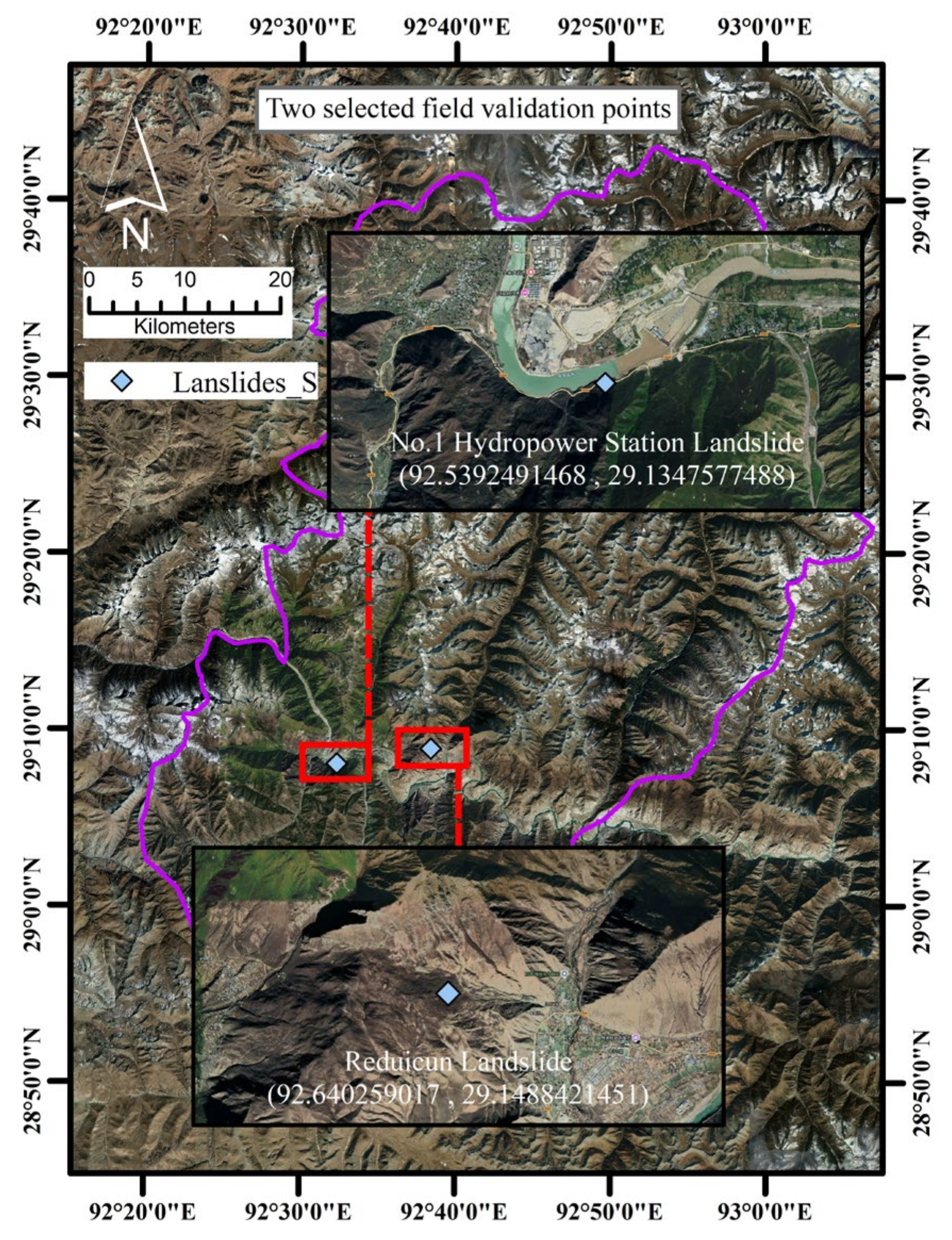
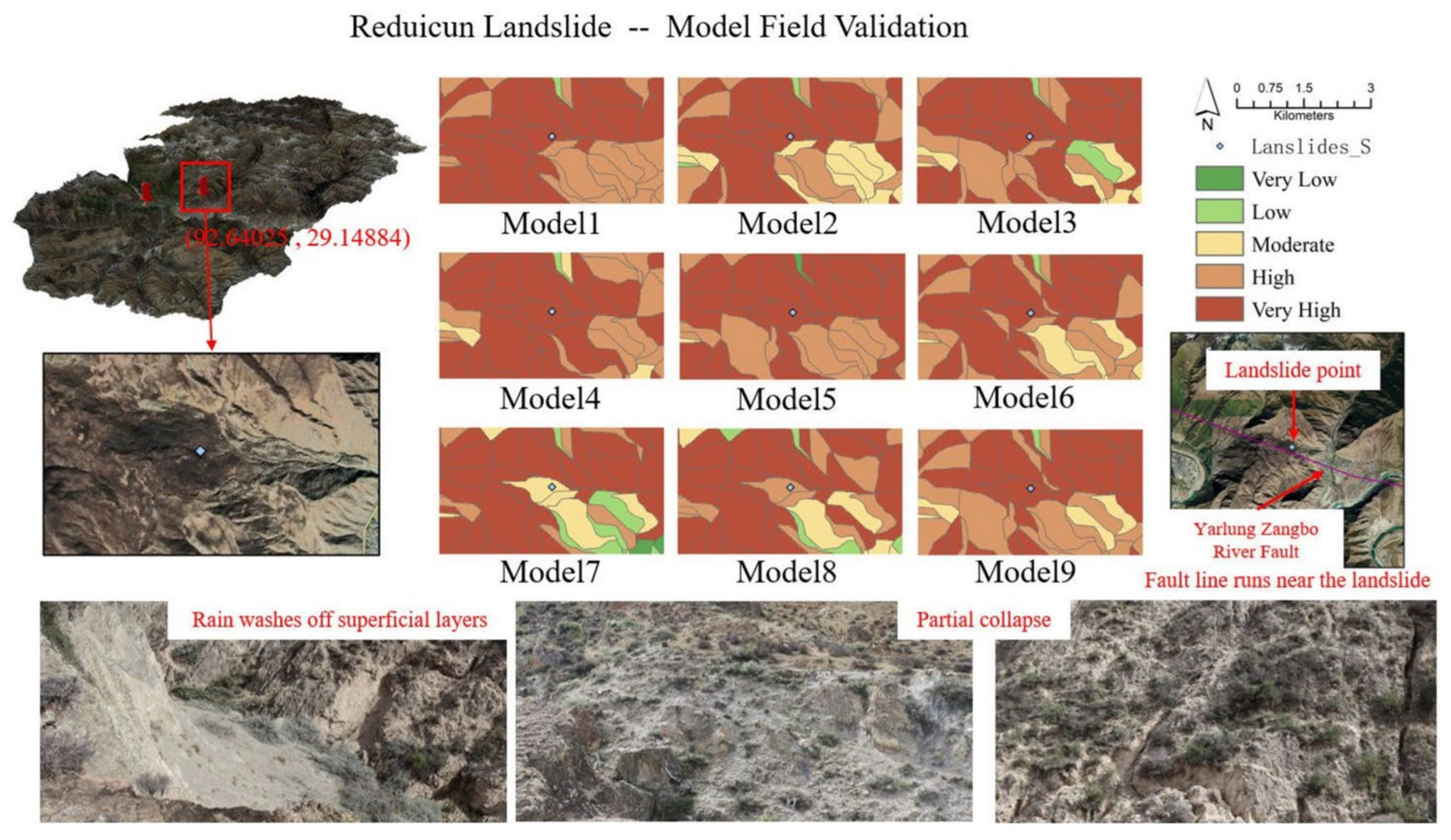
• The established model was utilized for landslide susceptibility mapping, and the model’s result was field validated in two cases: the No.1 Hydropower Station Landslide and the Reduicun Landslide. The model’s predicted results were found to be consistent with the actual situation to a certain extent, indicating that the susceptibility evaluation results obtained through this method have a degree of applicability and credibility. The integration of predicted results from multiple models can enhance the accuracy of susceptibility evaluation and provide a scientific foundation for disaster prevention and mitigation strategies in local contexts.

References

1. Assilzadeh, H.; Levy, J.K.; Wang, X. Landslide catastrophes and disaster risk reduction: A GIS framework for landslide prevention and management. Remote Sens. 2010, 2, 2259–2273. [Google Scholar] [CrossRef]
2. Wang, Y.; Sun, X.; Wen, T.; Wang, L. Step-like displacement prediction of reservoir landslides based on a metaheuristic-optimized KELM: A comparative study. Bull. Eng. Geol. Environ. 2024, 83, 322. [Google Scholar]
3. Wang, Y.; Jin, J.; Yuan, R. Analysis on Spatial Distribution and Influencing Factors of Geological Disasters in Southeast Tibet. J. Seismol. Res. 2019, 42, 428–437. [Google Scholar]
4. Qi, T.; Meng, X.; Qing, F.; Zhao, Y.; Shi, W.; Chen, G.; Zhang, Y.; Li, Y.; Yue, D.; Su, X. Distribution and characteristics of large landslides in a fault zone: A case study of the NE Qinghai-Tibet Plateau. Geomorphology 2021, 379, 107592. [Google Scholar]
5. Ye, T.; Shi, P.; Cui, P. Integrated Disaster Risk Research of the Qinghai-Tibet Plateau Under Climate Change. Int. J. Disaster Risk Sci. 2023, 14, 507–509. [Google Scholar]
6. Wang, F.; Wen, Z.; Gao, Q.; Yu, Q.; Li, D.; Chen, L. Thermokarst landslides susceptibility evaluation across the permafrost region of the central Qinghai-Tibet Plateau: Integrating a machine learning model with InSAR technology. J. Hydrol. 2024, 642, 131800. [Google Scholar] [CrossRef]
7. Huang, F.; Cao, Y.; Li, W.; Catani, F.; Song, G.; Huang, J.; Yu, C. Uncertainties of landslide susceptibility prediction: Influences of different study area scales and mapping unit scales. Int. J. Coal Sci. Technol. 2024, 11, 143–172. [Google Scholar]
8. Fang, K.; Tang, H.; Li, C.; Su, X.; An, P.; Sun, S. Centrifuge modelling of landslides and landslide hazard mitigation: A review. Geosci. Front. 2023, 14, 101493. [Google Scholar]
9. Sethi, S.S.; Ewers, R.M.; Jones, N.S.; Orme, C.D.L.; Picinali, L. Robust, real-time and autonomous monitoring of ecosystems with an open, low-cost, networked device. Methods Ecol. Evol. 2018, 9, 2383–2387. [Google Scholar]
10. Huang, F.; Liu, K.; Li, Z.; Zhou, X.; Zeng, Z.; Li, W.; Huang, J.; Catani, F.; Chang, Z. Single landslide risk assessment considering rainfall-induced landslide hazard and the vulnerability of disaster-bearing body. Geol. J. 2024, 59, 2549–2565. [Google Scholar]
11. Zhang, J.; Lin, C.; Tang, H.; Wen, T.; Tannant, D.D.; Zhang, B. Input-parameter Optimization Using a SVR Based Ensemble Model to Predict Landslide Displacements in a Reservoir Area—A Comparative Study. Appl. Soft Comput. 2024, 150, 111107. [Google Scholar] [CrossRef]
12. Lv, L.; Chen, T.; Dou, J.; Plaza, A. A hybrid ensemble-based deep-learning framework for landslide susceptibility mapping. Int. J. Appl. Earth Obs. Geoinf. 2022, 108, 102713. [Google Scholar] [CrossRef]
13. Ullah, I.; Aslam, B.; Shah, S.H.I.A.; Tariq, A.; Qin, S.; Majeed, M.; Havenith, H.-B. An integrated approach of machine learning, remote sensing, and GIS data for the landslide susceptibility mapping. Land 2022, 11, 1265. [Google Scholar] [CrossRef]
14. Tripathi, A.; Tiwari, R.K.; Tiwari, S.P. A deep learning multi-layer perceptron and remote sensing approach for soil health based crop yield estimation. Int. J. Appl. Earth Obs. Geoinf. 2022, 113, 102959. [Google Scholar] [CrossRef]
15. Gao, D.; Li, K.; Cai, Y.; Wen, T. Landslide Displacement Prediction Based on Time Series and PSO-BP Model in Three Georges Reservoir, China. J. Earth Sci. 2024, 35, 1079–1082. [Google Scholar] [CrossRef]
16. Huang, F.; Liu, K.; Jiang, S.; Catani, F.; Liu, W.; Fan, X.; Huang, J. Optimization method of conditioning factors selection and combination for landslide susceptibility prediction. J. Rock Mech. Geotech. Eng. 2025, 17, 722–746. [Google Scholar] [CrossRef]
17. Cheng, H.; Zheng, Y.; Wu, S.; Lin, Y.; Gao, F.; Lin, D.; Wei, J.; Wang, S.; Shu, D.; Wei, S. GIS-based mineral prospectivity mapping using machine learning methods: A case study from Zhuonuo ore district, Tibet. Ore Geol. Rev. 2023, 161, 105627. [Google Scholar] [CrossRef]
18. Huang, F.; Mao, D.; Jiang, S.; Zhou, C.; Fan, X.; Zeng, Z.; Catani, F.; Yu, C.; Chang, Z.; Huang, J.; et al. Uncertainties in landslide susceptibility prediction modeling: A review on the incompleteness of landslide inventory and its influence rules. Geosci. Front. 2024, 15, 101886. [Google Scholar] [CrossRef]
19. Yang, Z.; Guo, C.; Wu, R.; Zhong, N.; Ren, S. Predicting seismic landslide hazard in the Batang fault zone of the Qinghai-Tibet Plateau. Hydrogeol. Eng. Geol. 2021, 48, 91–101. [Google Scholar] [CrossRef]
20. Yin, G.; Luo, J.; Niu, F.; Lin, Z.; Liu, M. Machine learning-based thermokarst landslide susceptibility modeling across the permafrost region on the Qinghai-Tibet Plateau. Landslides 2021, 18, 2639–2649. [Google Scholar] [CrossRef]
21. Lin, Q.; Steger, S.; Pittore, M.; Zhang, J.; Wang, L.; Jiang, T.; Wang, Y. Evaluation of potential changes in landslide susceptibility and landslide occurrence frequency in China under climate change. Sci. Total Environ. 2022, 850, 158049. [Google Scholar] [PubMed]
22. Zou, Z.; Luo, T.; Zhang, S.; Duan, H.; Li, S.; Wang, J.; Deng, Y.; Wang, J. A novel method to evaluate the time-dependent stability of reservoir landslides: Exemplified by Outang landslide in the Three Gorges Reservoir. Landslides 2023, 20, 1731–1746. [Google Scholar] [CrossRef]
23. Xie, Y.; Sun, W.; Ren, M.; Chen, S.; Huang, Z.; Pan, X. Stacking ensemble learning models for daily runoff prediction using 1D and 2D CNNs. Expert Syst. Appl. 2023, 217, 119469. [Google Scholar]
24. Divina, F.; Gilson, A.; Goméz-Vela, F.; García Torres, M.; Torres, J.F. Stacking ensemble learning for short-term electricity consumption forecasting. Energies 2018, 11, 949. [Google Scholar] [CrossRef]
25. Wang, Y.; Wang, D.; Geng, N.; Wang, Y.; Yin, Y.; Jin, Y. Stacking-based ensemble learning of decision trees for interpretable prostate cancer detection. Appl. Soft Comput. 2019, 77, 188–204. [Google Scholar]
26. Chen, J.; Zeb, A.; Nanehkaran, Y.A.; Zhang, D. Stacking ensemble model of deep learning for plant disease recognition. J. Ambient Intell. Humaniz. Comput. 2023, 14, 12359–12372. [Google Scholar] [CrossRef]
27. Duan, Z.; Zhang, L.; Xue, Y.; He, M.; Chen, J. Analysis of the development characteristics and influencing factors of landslide disasters in Hunan Province based on big data theory. China Min. Mag. 2024, 1–11. [Google Scholar]
28. Yan, G.; Liang, S.; Zhao, H. An Approach to Improving Slope Unit Division Using GIS Technique. Sci. Geogr. Sin. 2017, 37, 1764–1770. [Google Scholar] [CrossRef]
29. Nguyen, H.-P.; Liu, J.; Zio, E. A long-term prediction approach based on long short-term memory neural networks with automatic parameter optimization by Tree-structured Parzen Estimator and applied to time-series data of NPP steam generators. Appl. Soft Comput. 2020, 89, 106116. [Google Scholar]
30. Wei, L.; Cheng, N. Research on Web Log Abnormal Traffic Detection Based on the SVM-DT-MLP Model. Mod. Inf. Technol. 2024, 8, 171–174+179. [Google Scholar] [CrossRef]
31. Zhang, T.; Huang, Y.; Liao, H.; Liang, Y. A hybrid electric vehicle load classification and forecasting approach based on GBDT algorithm and temporal convolutional network. Appl. Energy 2023, 351, 121768. [Google Scholar]
32. Wan, M.; Zou, S. Adolescent mental health state assessment framework by combining YOLO with random forest. Appl. Soft Comput. 2024, 168, 112497. [Google Scholar]
33. Li, J.; Gao, L.; Li, P.; Zhang, X.; Yang, J.; Su, S. Detection of Imbalanced Multi-class False Data Injection Attacks in Cyber-physical Systems Based on DDPM-Light GBM. J. Kunming Univ. Sci. Technol. (Nat. Sci.) 2024, 1–12. [Google Scholar] [CrossRef]
34. Li, X.; Wang, L.; Sung, E. AdaBoost with SVM-based component classifiers. Eng. Appl. Artif. Intell. 2008, 21, 785–795. [Google Scholar]
35. Tian, R.; Li, S.; Liu, T.; Jing, Y. vP/vS prediction based on XGBoost algorithm and itsapplication in reservoir detection. Oil Geophys. Prospect. 2024, 59, 653–663. [Google Scholar] [CrossRef]
36. Zhang, S.; Zhang, J. Wind Power Load Combination Forecasting Based on Improved SOA and Ridge Regression Weighting. J. North China Electr. Power Univ. 2024, 51, 1–10. [Google Scholar]
37. Hajihosseinlou, M.; Maghsoudi, A.; Ghezelbash, R. Stacking: A novel data-driven ensemble machine learning strategy for prediction and mapping of Pb-Zn prospectivity in Varcheh district, west Iran. Expert Syst. Appl. 2024, 237, 121668. [Google Scholar] [CrossRef]
38. Wu, X.; Ren, F.; Niu, R.; Peng, L. Landslide Spatial Prediction Based on Slope Units and Support Vector Machines. Geomat. Inf. Sci. Wuhan Univ. 2013, 38, 1499–1503. [Google Scholar]
39. Liu, T.; Xu, L.; Yuan, K.; Yan, W. Constant Volume Method of Shared Bicycle Parking Area Based on Natural Breakpoint Method. J. Wuhan Univ. Technol. (Transp. Sci. Eng.) 2023, 47, 992–997. [Google Scholar]
Figure 1. Geographical location of the study area.
Remotesensing 17 01177 g001
Figure 2. Factors’ test heat map.
Remotesensing 17 01177 g002
Figure 3. Jiacha landslide conditioning factors.
Remotesensing 17 01177 g003aRemotesensing 17 01177 g003b
Figure 4. Comparison of condition factors’ distribution relation between the area and landslide points in Jiacha County. (Subfig (a) described the distribution relation of Elevation. Subfig (b) described the distribution relation of the distance to roads. Subfig (c) described the distribution relation of the distance to faults. Subfig (d) described the distribution relation of aspect. Subfig (e) described the distribution relation of EVI. Subfig (f) described the distribution relation of SPI. Subfig (g) described the distribution relation of Surface Curvature. Subfig (h) described the distribution relation of Profile Curvature. Subfig (i) described the distribution relation of lithology. For subfig (i), “APl” refers to “Acid Plutonics”, “AVo” refers to “Acid Volcanic”, “BPl” refers to “Basic Plutonics”, “BVo” refers to “Basic Volcanics”, “IPl” refers to “Intermediate Plutonics”, “IVo” refers to “Intermediate Volcanics”, “Meta” refers to “Metamorphics”, “MsR” refers to “Mixed-sedimentary Rock”, “SSe” refers to “Siliciclastic Sedimentary”, “USe” refers to “Unconsolidated Sediment”. Subfig (j) described the distribution relation of Annual average temperature. Subfig (k) described the distribution relation of slope angle. Subfig (l) described the distribution relation of TPI. Subfig (m) described the distribution relation of the distance to river. Subfig (n) described the distribution relation of slope unit area).
Remotesensing 17 01177 g004
Figure 5. Process overview in this study.
Remotesensing 17 01177 g005
Figure 6. Base model workflow.
Remotesensing 17 01177 g006
Figure 7. Stacking workflow.
Remotesensing 17 01177 g007
Figure 8. The confusion matrix on 9 outstanding model test sets.
Remotesensing 17 01177 g008
Figure 9. The confusion matrix on 9 outstanding model train sets.
Remotesensing 17 01177 g009aRemotesensing 17 01177 g009b
Figure 10. ROC curve for 9 outstanding models.
Remotesensing 17 01177 g010aRemotesensing 17 01177 g010b
Figure 11. Landslide susceptibility maps of 9 outstanding models. (For subfig (a), “Model1” is Ada+DT+GBDT+kNN+MLP+Ridge+SVC|Meta Model:RF. For subfig (b), “Model2” is Ada+DT+GBDT+kNN+MLP+Ridge+SVC|Meta Model:LGBM. For subfig (c), “Model3” is Ada+DT+GBDT+kNN+MLP+RF+Ridge+SVC|Meta Model:XGB. For subfig (d), “Model4” is Ada+DT+kNN+LGBM+MLP+RF+Ridge+SVC|Meta Model:GBDT. For subfig (e),” Model5” is Ada+DT+GBDT+LGBM+MLP+RF+Ridge+SVC|Meta Model:XGB. For subfig (f), “Model6” is Ada+DT+GBDT+kNN+LGBM+MLP+Ridge+SVC|Meta Model:XGB. For subfig (g), “Model7” is Ada+DT+GBDT+MLP+Ridge+SVC+XGB|Meta Model:LGBM. For subfig (h), “Model8” is Ada+DT+GBDT+kNN+MLP+Ridge+SVC+XGB|Meta Model:RF. For subfig (i), “Model9” is Ada+DT+kNN+LGBM+MLP+RF+Ridge+SVC|Meta Model:XGB).
Remotesensing 17 01177 g011aRemotesensing 17 01177 g011b
Figure 12. Typical landslide location selected. (Satellite map from Google Earth, 2022).
Remotesensing 17 01177 g012
Figure 13. Localized map of landslide susceptibility and field verification of No.1 Hydropower Station Landslide.
Remotesensing 17 01177 g013
Figure 14. Localized map of landslide susceptibility and field verification of Reduicun Landslide.
Remotesensing 17 01177 g014