Prediction of Vanadium Contamination Distribution Pattern Through Remote Sensing Image Fusion and Machine Learning

Abstract

Soil vanadium contamination poses a significant threat to ecosystems. Hyperspectral remote sensing plays a critical role in extracting spectral features of heavy metal contamination, mapping its spatial distribution, and monitoring its trends over time. This study targets a vanadium-contaminated area in Panzhihua City, Sichuan Province. Soil sampling and spectral measurements occurred in the laboratory. Hyperspectral (Gaofen-5, GF-5) and multispectral (Gaofen-2, GF-2; Sentinel-2) images were acquired and preprocessed, and feature bands were extracted by combining laboratory spectral data. A dual-branch convolutional neural network (DB-CNN) fused hyperspectral and multispectral images and confirmed the fusion’s effectiveness. Six prevalent machine learning models were adopted, and a unified learning framework leveraged a Random Forest (RF) as a second-layer model to enhance the predictive performance of these base models. Both the base models and the ensemble learning model were evaluated based on predictive accuracy. The fusion process enhanced the predictive performance of the base models, improving R² values for vanadium (V) and pentavalent vanadium (V5+) from 0.54 and 0.3 to 0.58 and 0.39, respectively, at a 4 m resolution. Further optimization using RF as a second-layer model to refine Extreme Trees (ETs) significantly increased R² values to 0.83 and 0.75 for V and V5+, respectively, at this scale. The 934 nm and 464 nm wavelengths were identified as the most critical spectral bands for predicting soil vanadium contamination. This integrated approach robustly delineates the spatial distribution characteristics of V and V5+ in soils, facilitating precise monitoring and ecological risk assessments of vanadium contamination through a comparative analysis of predictive accuracy across diverse models.

1. Introduction

The equilibrium between humanity and the natural environment is essential for sustainable development. However, heavy metal pollution caused by industrialization significantly disrupts this balance. Heavy metals in soil are poisonous and persistent, build up over time, and defy natural degradation, hence constituting a significant hazard to ecosystems [1,2]. Vanadium (V), a heavy metal extensively utilized in industry, accumulates in soil predominantly by mining and smelting [3,4]. Among the several oxidation states of vanadium, pentavalent vanadium (V5+) is the most poisonous and presents a significant ecological hazard [5,6]. Panzhihua, a region significantly impacted by vanadium pollution, is extremely susceptible to ecological degradation and poses potential health risks to humans [7,8,9]. Therefore, precise monitoring of the spatial distribution and dynamic variations of both V and V5+ is crucial for understanding their environmental impact and holds profound significance for protecting public health [10].

Geochemical methodologies, spatial interpolation techniques, and remote sensing technologies are predominantly employed to investigate heavy metal contamination in soil [11]. Geochemical methods provide significant accuracy; nevertheless, their utilization is constrained by environmental contamination from chemicals and the substantial time and labor demands of the process [12]. Geographic interpolation methods suffer from low predictive accuracy due to the high heterogeneity of heavy metal spatial distribution and the sampling intervals at boundary regions [13,14]. Remote sensing techniques establish a quantitative relationship between soil spectral characteristics and heavy metal concentrations [15], offering distinct advantages, such as rapid spectral sampling and non-destructive environmental monitoring, enabling large-scale assessments [16]. In terms of sensors, satellite-based MS and HS imagery are two commonly used data sources, with HS often achieving better predictive accuracy due to its finer spectral resolution. For instance, Song et al. [17] utilized Landsat 7 ETM+ and Landsat 8 OLI multispectral imagery to predict Ni content in agricultural soils of Wuqing District, Tianjin, constrained by the limited number of spectral bands, which hinders the development of diverse spectral transformations, achieving a relatively good predictive accuracy (R² = 0.69). In contrast, Sun et al. [18] employed Zhuhai-1 OHS imagery to delineate the spatial distribution of soil nickel over an area of approximately 13,300 km² on the Leizhou Peninsula, achieving a higher level of predictive accuracy (R² = 0.8, RPD = 2.08). In recent years, with the continuous progress in feature selection [19], prediction methods [20], and spectral indices [21], the predictive accuracy of HS remote sensing has steadily improved, gradually making it the dominant method for forecasting the distribution of heavy metals in soil [22].

Hyperspectral sensors typically enhance spectral sampling at the expense of spatial resolution due to the inherent trade-off between these two dimensions [23,24]. Current hyperspectral prediction research commonly employs raw HS data as the input, a widely adopted practice. The superior spectral resolution of GF-5B has been shown to improve modeling accuracy; however, its lower spatial resolution restricts detailed monitoring of complex land use types [25,26]. To enhance the reliability of HS predictions, a common approach is multi-source data fusion, which enriches the feature set to boost prediction accuracy [27]. For instance, Zhou et al. [28] fused UAV-based hyperspectral, Sentinel-2 multispectral, and SAR data, increasing the R² for soil arsenic prediction from 0.4–0.6 to 0.71. Yet, this method falls short of achieving a fine-scale pollution prediction. To address this limitation, image-based feature fusion integrates high-resolution MS data with HS data acquired concurrently in the same spatial domain, thereby improving the spatial resolution of HS data and enhancing the model’s ability to represent complex features [29,30]. For example, Song et al. [31] utilized a deep feature fusion network to refine the original HS spatial resolution from 20 m to 1.3 m, raising classification accuracy from approximately 85% to 98%. Image fusion methods can be classified into pansharpening, decomposition, and machine-learning-based strategies [32]. Notably, dual-branch convolutional networks extract image features to produce high-quality fused images, making them well-suited for predicting elemental concentrations at fine scales [33,34,35].

Machine learning techniques have been extensively utilized for the prediction of heavy metals in HS data [36,37]. Traditional machine learning algorithms, however, are susceptible to overfitting and spatial autocorrelation, hence amplifying prediction uncertainty [38,39]. Ensemble learning integrates several base models to utilize their complementing strengths and error correction capabilities, therefore reducing the influence of individual model mistakes and significantly improving predictive performance [40,41]. The random forest model is extensively utilized among ensemble learning methods due to its adaptable framework and capacity to address nonlinear issues [42,43]. The multi-tree architecture mitigates random mistakes in individual trees via averaging, hence enhancing the model’s overall robustness. Nevertheless, current research has insufficiently addressed how random forests reconcile local and global information in error correction, hence constraining their efficacy in predicting hyperspectral heavy metal pollution.

This research examines the heavily vanadium-contaminated area of Panzhihua, Sichuan Province, utilizing data from 211 soil heavy metal survey locations after outlier removal. We constructed a framework by integrating HS and MS data, utilizing DB-CNN and RF to enhance the base model. This method tackles critical technological issues in spectral feature extraction, precise modeling, and spatial mapping concerning soil vanadium pollution. Specific research tasks encompass (1) extracting critical spectral features for V and V5+ via spectral preprocessing and correlation analysis and identifying highly correlated heavy metals through associated element analysis; (2) executing hyperspectral and multispectral data fusion utilizing DB-CNN to enhance spatial resolution and feature count; (3) optimizing the predictive performance of various traditional machine learning models and selecting the most effective model; (4) constructing an RF ensemble framework to significantly enhance prediction accuracy by minimizing the prediction errors of the base model. The results of this study provide crucial insights for the accurate monitoring of V and V5+, with broad application potential, especially for regional pollution monitoring in complex environments.

The technical workflow of this study is illustrated in Figure 1, which includes four main steps: feature extraction, image fusion, model construction, and spatial mapping.

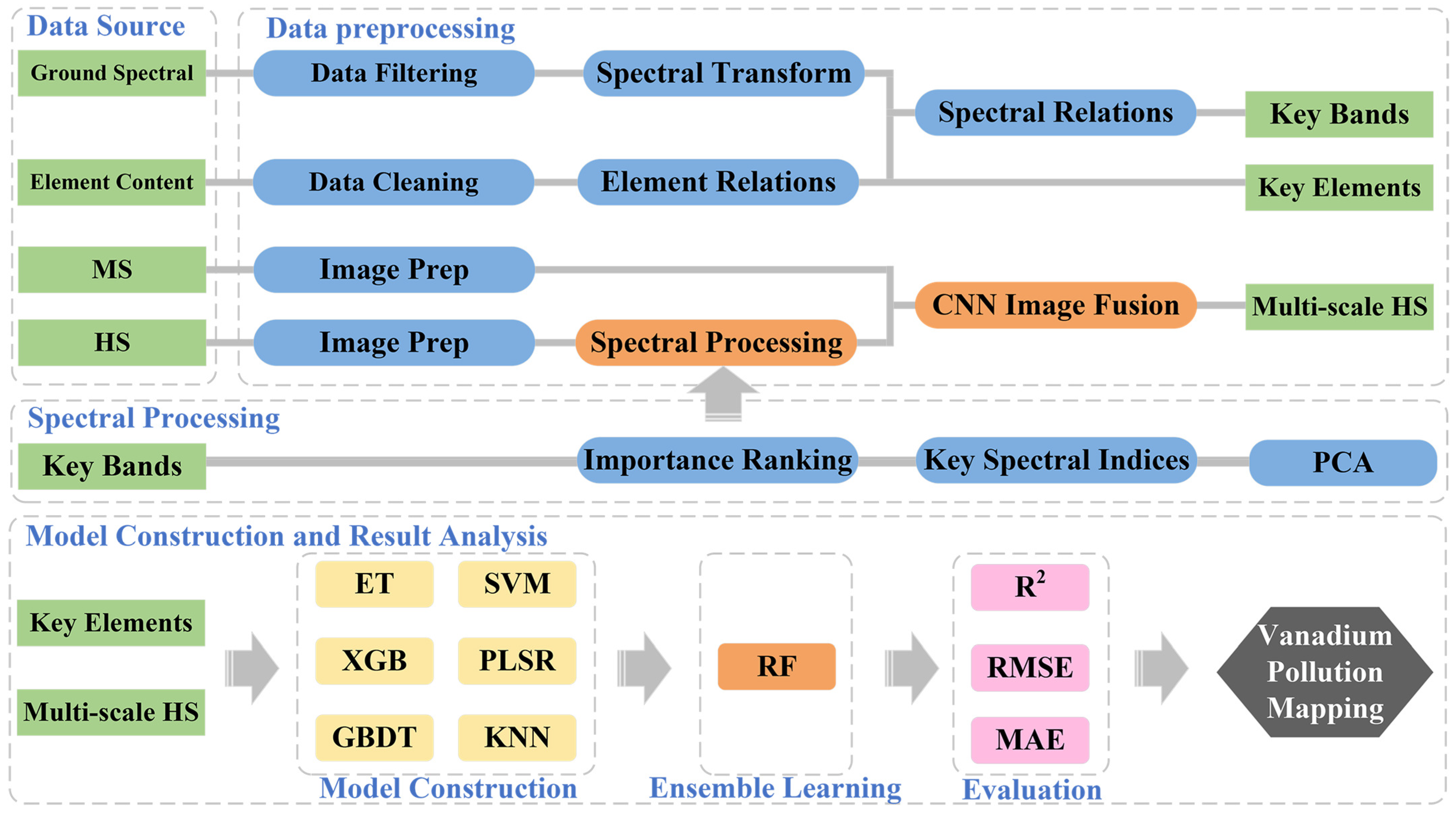
2. Materials and Methods

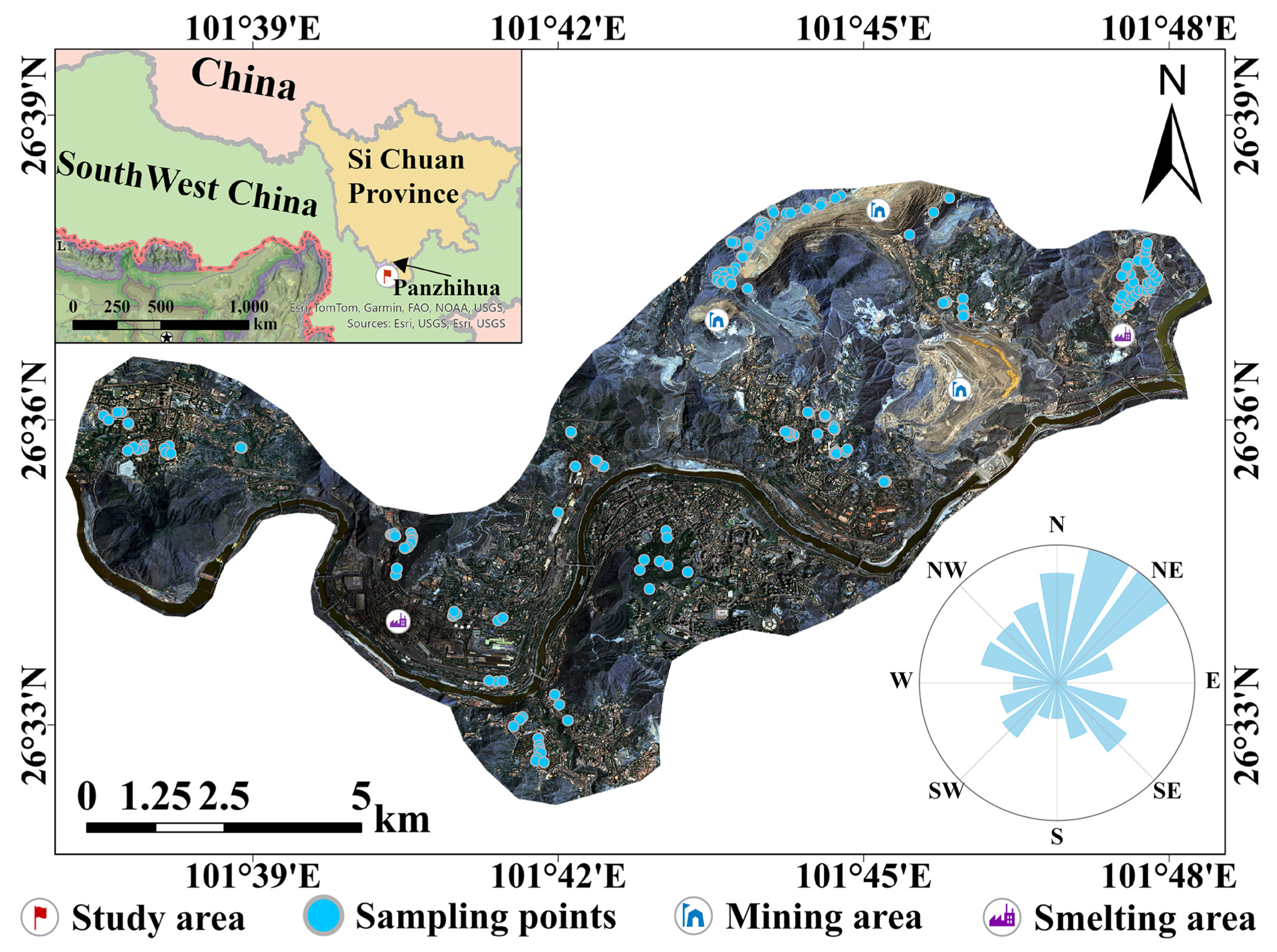
2.1. Overview of the Study Area

The study area is situated in Panzhihua City, southern Sichuan Province, China, within the subtropical dry–hot valley climate zone, characterized by prevailing southwest winds. This region, with its complex and diverse terrain, is a key base for the vanadium–titanium industry in southwest China. It has a long history of mining and smelting activities [44], which have significantly affected the local ecological environment. The study area spans from 26°31′ to 26°38′N and 101°37′ to 101°48′E (Figure 2), covering mining and smelting zones, urban areas, forests, and farmlands, with the agricultural area primarily dedicated to the cultivation of economic crops. All these areas are associated with pollution sources and potential contamination. Soil samples were collected from bare ground across different soil types to minimize environmental disturbance and improve the accuracy and relevance of spectral data. The collected soil samples were passed through a 100-mesh sieve, ground, and air-dried naturally before being divided by weight into two portions for spectral measurements and elemental analysis.

2.2. Data Acquisition

2.2.1. Soil Investigation Data

Soil samples from the surface layer (0–20 cm depth) were collected at 248 survey points between 10 April 2023 and 13 April 2023 (Figure 2). In the mining and smelting areas, sampling points were evenly distributed along the entire regional boundary at intervals of 400–500 m. In farmland areas, the sampling layout combined the grid method and the plum blossom method. In urban and forest areas, the sampling density was determined according to the Technical Specifications for Soil Environmental Monitoring (HJ/T166-2004) [45]. Large stones, plant roots, and other debris were removed before the soil was placed in sampling bags and properly labeled. All sampling points were accurately located using handheld GPS devices. The collected soil samples were sieved through a 100-mesh screen, ground, and dried. The samples were then divided by weight into two portions: one for spectral analysis and the other for elemental analysis.

The spectral reflectance data were measured using an ATP9110 broadband spectral radiometer (Aopu Tiancheng, Xiamen, China) with sampling intervals of 350–900 nm (0.5 nm), 900–1200 nm (1 nm), and 1200–2500 nm (3 nm). Before measurements, the instrument was calibrated using a whiteboard and dark current measurements to eliminate background interference. The light source was a halogen lamp with a 60° angle of incidence positioned 30 cm above the sample surface, and the probe was held vertically above the sample. Each sample was measured five times, and after each measurement, the sample container was rotated 90° to minimize anisotropic effects. The average reflectance value from all directions was used as the final value.

The spectral reflectance was calculated using the following formula:

$$\begin{array}{c}R\left(\lambda \right)={\displaystyle \frac{S\left(\lambda \right)-D\left(\lambda \right)}{W\left(\lambda \right)-D\left(\lambda \right)}}\end{array}$$

(1)

Specifically, $\mathrm{S}\left(\mathsf{\lambda }\right)$ is the observed value of the target sample at the wavelength, $D\left(\mathsf{\lambda }\right)$ is the background noise at the wavelength, and $W\left(\mathsf{\lambda }\right)$ is the observed value of the standard reflectance plate at the wavelength.

The obtained spectral reflectance data were processed using SG filtering [46], followed by outlier detection and removal using the Isolation Forest method [47]. Feature transformations were carried out using a first-order derivative (FD), second-order derivative (SD), and maximum–minimum normalization (MMN). The final feature spectrum of the target was selected based on the correlation coefficients.

Elemental content was determined using the potassium permanganate oxidation–ammonium ferrous sulfate titration method for V and V5+ concentrations, and inductively coupled plasma mass spectrometry (ICP-MS; PerkinElmer, China) was used to determine the concentrations of the associated elements (Ti, Fe, Cr, Ni, Pb, Cu, Mn, Ca, and Zn). Outliers in the measurement samples were removed using the interquartile range method, and the elemental content data were obtained.

2.2.2. Remote Sensing Data

In this study, MS data from Sentinel-2A and GF-2 and HS data from GF-5B are used, and image fusion techniques are applied to preserve the spectral information of the HS data while taking advantage of the high spatial resolution of the MS data.

The GF-5B satellite, developed as the successor to China’s first hyperspectral remote sensing satellite, GF-5, has found extensive application in studies mapping soil heavy metal pollution [48,49,50]. It carries the Advanced Hyperspectral Imager (AHSI), which spans a spectral range of 400–2500 nm and provides a spatial resolution of 30 m. In the visible and near-infrared (VNIR) region, the AHSI acquires 150 bands with a sampling interval of 5 nm and a signal-to-noise ratio (SNR) of approximately 700. In the shortwave infrared (SWIR) region, it collects 180 bands at a 10 nm sampling interval, with an SNR of around 500 [51].

As China’s first sub-meter optical remote sensing satellite, GF-2 is equipped with a multispectral camera (MSS) that provides a spatial resolution of 4 m, making it highly suitable for the fusion of HS and MS data [52].

Sentinel-2A (S2A) data were acquired through the Google Earth Engine (GEE) platform, with the dataset being COPERNICUS/S2_SR_HARMONIZED. The spatial resolution of the RGB bands is 10 m. The data have undergone preprocessing steps such as radiometric calibration, atmospheric correction, and cloud removal. GF-2 data were provided by the China Resource Satellite Center, and the acquisition method for GF-5B data is the same as for GF-2. Radiometric calibration and FLAASH atmospheric correction were performed on both datasets in ENVI 5.6 (Harris Geospatial Solutions, Broomfield, CO, USA). After atmospheric correction, the GF-5B data retained 312 usable bands, which were further processed using SG filtering and smooth normalization techniques. For geometric correction, GF-2 images were georeferenced using RPC files and ALOS-PALSAR DEM, while GF-5B and S2A images were resampled using the nearest neighbor interpolation method and georeferenced to the corrected GF-2 images. The geometric error was controlled to within 0.5 pixels in ENVI 5.6. To meet the requirements for image fusion, we subsequently resampled the GF-5B imagery to generate datasets with spatial resolutions of 30 m, 10 m, and 4 m, corresponding to the original spatial resolutions of GF-5B, Sentinel-2A, and GF-2, respectively. The 30 m scale was designated as the control group, while the 10 m and 4 m scales served as the experimental groups for image fusion. We retained the RGB bands from Sentinel-2A and GF-2 as the multispectral input for the fusion process. The remote sensing data sources used in this study are summarized in

Table 1. Remote sensing data sources were utilized in this study.

Type	Data	Data ID	Date
HS	GF-5B	GF5B_AHSI_E101.8_N26.4_20230413_008494_L10000316410	13 April 2023
MS	Sentinel-2A	20230409T034541_20230409T040008_T47RQK	9 April 2023
	GF-2	GF2_PMS1_E101.5_N26.5_20230410_L1A0007216553	10 April 2023
		GF2_PMS2_E101.7_N26.5_20230410_L1A0007216706
		GF2_PMS2_E101.8_N26.7_20230410_L1A0007216704

.

2.3. Characteristic Band Extraction

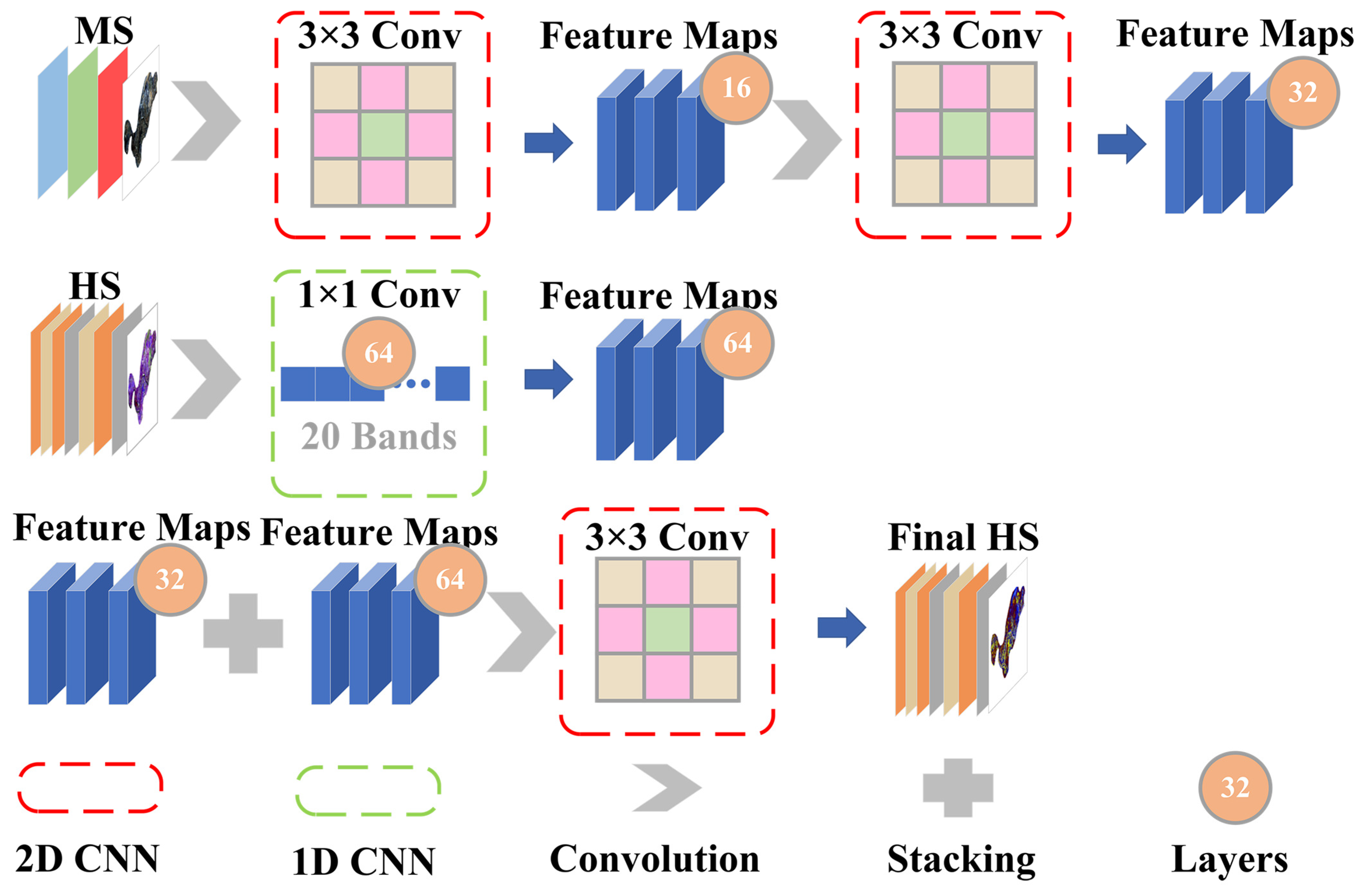
This study references the indirect prediction method proposed by Shen et al. [53], which explores the feasibility of indirectly estimating the concentration of target elements by extracting the spectral features of related elements based on the spectral correlation between the target element and its associated elements. Building on this approach, we extract feature bands from GF-5B hyperspectral data through two stages. Initially, Pearson correlation analysis evaluates correlations among element concentrations and between them and spectral reflectance, identifying significant elements for V and V5+ and their spectral response ranges. Subsequently, RF is employed to rank the importance of features, retaining the top 20 most important bands for HS input.

2.4. Image Fusion

The DB-CNN model was employed, with the HS spectral bands resampled and aligned with the MS data. The model uses a 2D CNN to extract spatial features from the MS data and a 1D CNN to extract spectral features from the HS data. In the fusion model, the activation function was used to ensure that all features are positive, thus improving the ability of the model to capture nonlinear representations [34,54,55]. The procedure is shown in Figure 3.

To extract spatial features from the MS, a 3 × 3 convolution kernel was applied, using two convolution operations to capture spatial information, as shown in Equation (2).

$$\begin{array}{c}MS=ReLU\left({\mathrm{Conv}}_{3\times 3}^{16\to 32}\left(ReLU\left({\mathrm{Conv}}_{3\times 3}^{3\to 16}\left(M{S}_{\mathrm{RGB}}\right)\right)\right)\right)\end{array}$$

(2)

To extract spectral features from HS, a 1 × 1 convolution kernel was applied to aggregate the spectral information [56], as shown in Equation (3).

$$\begin{array}{c}HS=ReLU\left({\mathrm{Conv}}_{1\times 1}^{20\to 64}\left(H{S}_f\right)\right)\end{array}$$

(3)

By concatenating the spatial features of the MS with the spectral features of the HS, the fused feature map $F_f$ is obtained, as shown in Equation (4).

$$\begin{array}{c}{F}_f=\{MS,HS\}\end{array}$$

(4)

A 3 × 3 convolutional kernel is applied to the fused feature map $F_f$. where the number of channels is reduced to match the number of bands in the input HS, resulting in the fused HS image, as shown in Equation (5) [57].

$$\begin{array}{c}\mathrm{O}\mathrm{u}\mathrm{t}\mathrm{p}\mathrm{u}\mathrm{t}=ReLU\left({\mathrm{Conv}}_{3\times 3}^{96\to 20}\left(F_f\right)\right)\end{array}$$

(5)

Specifically, $M{S}_{\mathrm{RGB}}$ indicates the RGB bands of the input MS, $H{S}_f$ represents the important bands of the input HS, and $\mathrm{Conv}$ is the convolution operation.

To evaluate the effectiveness of image fusion, a qualitative evaluation was performed by comparing the details of the images before and after fusion [58]. A peak signal-to-noise ratio (PSNR), structural similarity index (SSIM), and feature similarity index (FSIM) were used as quantitative evaluation metrics. Previous studies have shown that a PSNR greater than 30 dB and SSIM and FSIM values close to 1 indicate good fusion results [29,59,60]. The calculation formulas are given in Equations (6)–(8):

$$\begin{array}{c}PSNR=10\cdot {\log }_{10}\left({\displaystyle \frac{{\mathrm{Max}}^2}{\frac{1}{\mathrm{n}}{\sum }_{\mathrm{i}=1}^{\mathrm{N}}{\left(y_i-\widehat{y_i}\right)}^2}}\right)\end{array}$$

(6)

$$\begin{array}{c}SSIM\left(a,b\right)={\displaystyle \frac{\left(2{\mu }_a{\mu }_b+ C_1\right)\left(2{\sigma }_{ab} + C_2\right)}{\left({\mu }_a^2 + {\mu }_b^2 + C_1\right)\left({\sigma }_a^2 + {\sigma }_b^2 + C_2\right)}}\end{array}$$

(7)

$$\begin{array}{c}FSIM\left(a,b\right)={\displaystyle \frac{{\sum }_{i\in \mathsf{\Omega }}{S}_L\left(i\right)\cdot P{C}_m\left(i\right)}{{\sum }_{i\in \mathsf{\Omega }}P{C}_m\left(i\right)}}\end{array}$$

(8)

The following parameters are defined: $\mathrm{Max}$ is the maximum pixel value of the image, $y_i$ represents the observed value, $\widehat{y_i}$ is the predicted value, and $\mathrm{n}$ is the sample size. $a$ and $b$ represent the HS images before and after fusion, respectively. ${\mu }_a$ and ${\mu }_b$ are the average brightness values of the pre- and post-fusion images, while ${\sigma }_a^2$ and ${\sigma }_b^2$ denote the brightness variances of the pre- and post-fusion images, respectively. ${\sigma }_{ab}$ represents the brightness covariance between the pre- and post-fusion images. $C_1$ and $C_2$ are constants introduced to avoid a zero denominator. In this study, $C_1={\left(0.01L\right)}^2$ and $C_2={\left(0.03L\right)}^2$, where $i\in \mathsf{\Omega }$ represents the pixel value range. $S_L\left(i\right)$ denotes the local similarity, $P{C}_m\left(i\right)$ represents the local feature weight, and $\mathsf{\Omega }$ refers to the pixel set.

2.5. Construction of Spectral Indices

In this study, spectral indices are constructed based on the importance ranking of the bands. The feature bands corresponding to each element are selected to construct the indices, with the aim of better capturing the characteristics of the features and improving the accuracy of the model. For instance, NDVI, calculated as the ratio of Near Infrared (NIR) to Red Band (R), more effectively reduces atmospheric scattering interference and enhances vegetation classification accuracy compared to using a single band [61]. According to the study of Jia et al. [62], the spectral indices are constructed in the following order: Normalized Difference (ND), Multiplicative Product (MP), Ratio (RT), Square Root Product (SP), Logarithmic (ALN), and Sum of Squares (SB). The construction methods are shown in

Table 2. Construction methods of spectral indices.

Order	Method	Combination
1	ND	$\left(a-b\right)/\left(a+b\right)$
2	MP	$a\times b$
3	RT	${\displaystyle \frac{a}{b}}$
4	SP	$\sqrt{a^2+b^2}$
5	ALN	$ln\left(a\right)$
6	SB	$\sqrt{\left|a^2-b^2\right|}$

Specifically, $a$ and $b$ represent two different bands randomly selected from the 20 characteristic bands.

, with dimensionality reduction performed using Principal Component Analysis (PCA) at a 95% level of variance explanation.

2.6. Model Building Methods

2.6.1. Ensemble Learning

This study compares six traditional machine learning models for their building effectiveness, including Extremely Randomized Trees (ETs), Extreme Gradient Boosting (XGB), Gradient Boosting Decision Trees (GBDTs), Support Vector Machines (SVMs), k-nearest Neighbors (KNNs), and Partial Least Squares Regression (PLSR). We also explore the performance of an RF in optimizing the base models. An ET randomly generates candidate feature splitting points and selects the best rule by training decision trees on the sample set, ensuring efficient training [63]. XGB applies regularization, iteratively adds decision trees, and performs feature splitting by summing leaf node scores to generate new features, reducing prediction variance and avoiding overfitting [64]. A GBDT trains weak regressors in iterations, adjusting the errors from the previous regression tree, which effectively improves the learning and generalization ability of the model [65]. An SVM maps the data into a high-dimensional space using kernel functions and performs regression analysis over a maximum margin hyperplane, which is suitable for handling high-dimensional data [66]. PLSR converts highly correlated predictors into simplified orthogonal latent components, which significantly improves the correlation with the response variable, making it suitable for handling HS data with highly correlated predictors [67]. KNN predicts new data points by computing a weighted average of the K nearest neighbors in the training set, making it effective for handling high-noise data [68]. An RF generates decision trees from multiple bootstrap samples and performs subset variable selection at each node, ensuring simplicity and reliability [69]. As a second-layer ensemble model, the RF demonstrates excellent performance [40].

The model construction process begins by using spectral transformations to extract key principal components from hyperspectral remote sensing data. These components serve as inputs to the six base models, which generate initial predictions ${\widehat{y}}_1$. An RF is then employed to optimize prediction errors by modeling the residuals $y-{\widehat{y}}_1$. Inspired by boosting algorithms in ensemble learning, a learning rate $\alpha$ is introduced to scale the residual correction, resulting in optimized predictions ${\widehat{y}}_2$. The hyperparameters of both the base models and RF, along with $\alpha$, are fine-tuned using Bayesian optimization with five-fold cross-validation to ensure robust and stable model performance. The model construction and optimization processes were implemented using the scikit-learn library (v1.6.2) in a Python 3.12 environment. The hyperparameter search ranges are detailed in Table 3. The calculation formula is as follows:

$$\begin{array}{c}{\widehat{y}}_2={\widehat{y}}_1+\alpha \cdot f_{\mathrm{RF}}\left(y-{\widehat{y}}_1\right)\end{array}$$

(9)

Specifically, $f_{\mathrm{RF}}\left(y-{\widehat{y}}_1\right)$ represents the RF prediction function for the error term $y-{\widehat{y}}_1$, and $\alpha$ represents the learning rate, automatically optimized within the range [0.1, 1.0] using Bayesian optimization.

Table 3. Hyperparameter search ranges for base models and random forest optimization.

Model	Parameter	Search Range
ET	n_estimators	[100, 300]
	max_depth	[5, 15]
	min_samples_split	[2, 10]
	min_samples_leaf	[1, 4]
XGB	learning_rate	[0.01, 0.3]
	n_estimators	[100, 300]
	max_depth	[3, 9]
	reg_alpha	[0, 10]
	reg_lambda	[1, 20]
	min_child_weight	[1, 5]
GBDT	n_estimators	[100, 300]
	max_depth	[3, 7]
	learning_rate	[0.01, 0.3]
SVR	C	[1, 100]
	gamma	[0.001, 1]
	epsilon	[0.05, 0.5]
PLSR	n_components	[2, 8]
RF	n_estimators	[100, 300]
	max_depth	[5, 15]
	min_samples_split	[2, 10]
	min_samples_leaf	[1, 4]
	alpha	[0.1, 1.0]

Table 3. Hyperparameter search ranges for base models and random forest optimization.

Model	Parameter	Search Range
ET	n_estimators	[100, 300]
	max_depth	[5, 15]
	min_samples_split	[2, 10]
	min_samples_leaf	[1, 4]
XGB	learning_rate	[0.01, 0.3]
	n_estimators	[100, 300]
	max_depth	[3, 9]
	reg_alpha	[0, 10]
	reg_lambda	[1, 20]
	min_child_weight	[1, 5]
GBDT	n_estimators	[100, 300]
	max_depth	[3, 7]
	learning_rate	[0.01, 0.3]
SVR	C	[1, 100]
	gamma	[0.001, 1]
	epsilon	[0.05, 0.5]
PLSR	n_components	[2, 8]
RF	n_estimators	[100, 300]
	max_depth	[5, 15]
	min_samples_split	[2, 10]
	min_samples_leaf	[1, 4]
	alpha	[0.1, 1.0]

2.6.2. Model Evaluation

The stratified sampling method based on quartiles was applied to the observational data of V and V5+, which was then split into a training set and a validation set at an 80%:20% ratio. Model evaluation was performed using the coefficient of determination (R²), residual prediction deviation (RPD), and mean absolute error (MAE) as performance metrics. The coefficient of determination (R²) assesses the model’s ability to explain the target variable. Residual prediction deviation (RPD) evaluates the consistency between predicted and measured values by calculating the ratio of the standard deviation (SD) to the root mean square error (RMSE), where RPD > 2.0 indicates good consistency, 1.4 < RPD < 2.0 indicates moderate consistency, and RPD < 1.4 indicates poor consistency. Mean absolute error (MAE) measures the average absolute difference between predicted and actual values. The formulas are as follows:

$$\begin{array}{c}{R}^2 = 1 - {\displaystyle \frac{{\left(y_i - \widehat{y_i}\right)}^2}{{\left(y_i - \overline{y}\right)}^2}}\end{array}$$

(10)

$$\begin{array}{c}RPD={\displaystyle \frac{\sqrt{\frac{1}{n-1}{\sum }_{i=1}^n{\left(y_i-\overline{y}\right)}^2}}{\frac{1}{n}{\sum }_{i=1}^n\left|y_i-\widehat{y_i}\right|}}\end{array}$$

(11)

$$\begin{array}{c}MAE={\displaystyle \frac{1}{n}}{\displaystyle \sum _{i=1}^n}\left|y_i-\widehat{y_i}\right|\end{array}$$

(12)

Specifically, $y_i$ represents the observed value for the sample, $\widehat{y_i}$ represents the predicted value, $\overline{y}$ represents the mean of observed values, $\left(y_i - \widehat{y_i}\right)$ represents the prediction residual, $\left|y_i-\widehat{y_i}\right|$ represents the absolute prediction error, and $n$ represents the total number of samples.

2.7. Spatial Mapping

In this study, bare soil areas within urban built-up zones, forests, and agricultural lands were delineated by integrating the remote sensing indices NDVI and NDBI. The NDVI, which is calculated as the difference between red and near-infrared bands, reflects the degree of vegetation cover in a region [70]. On the other hand, the NDBI, derived from the difference between shortwave infrared and near-infrared bands, indicates the distribution of built-up areas [71]. These indices were calculated using Sentinel-2A bands B4 (red), B8 (near-infrared), and B11 (shortwave infrared), as obtained from Table 1. Following Guha et al. [72], thresholds of NDVI < 0.2 and NDBI < 0.1 were set to identify bare soil areas, and a mask was applied to the model mapping results. The formulas are as follows:

$$\begin{array}{c}NDVI={\displaystyle \frac{\left(B8-B4\right)}{\left(B8+B4\right)}}\end{array}$$

(13)

$$\begin{array}{c}NDBI={\displaystyle \frac{\left(B11-B8\right)}{\left(B11+B8\right)}}\end{array}$$

(14)

3. Results

3.1. Feature Extraction

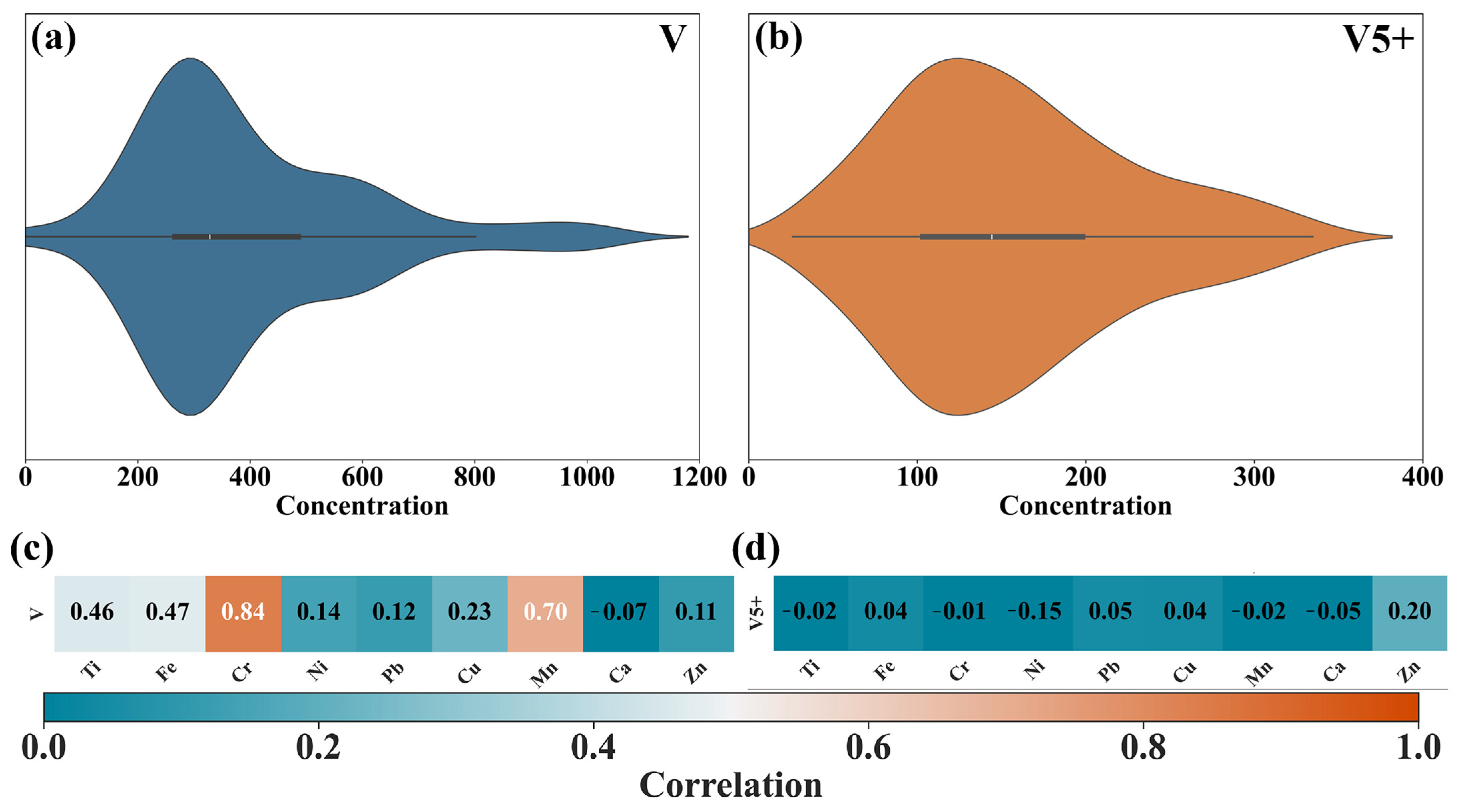
3.1.1. Soil Element Content Analysis

Out of the original 248 soil samples collected, outliers were removed using the interquartile range (IQR) method, reducing the number of survey points to 211. The statistical characteristics of V and V5+ in the soil samples, after outlier removal, are summarized in

Table 4. Basic statistical summary of V and V5+ concentrations.

Statistic	Unit	V	V5+
Max	mg/kg	1041.37	324.15
Min	mg/kg	0.00	26.10
Mean	mg/kg	396.72	154.41
Std	mg/kg	204.67	69.34
CV	%	51.59	44.91

. The content ranges of V and V5+ were 0–1041.37 mg/kg and 26.10–324.15 mg/kg, with mean values of 396.72 mg/kg and 154.41 mg/kg, respectively. The content and mean value of V were significantly higher than the soil background value and the global average V content (82 mg/kg and 103 mg/kg, respectively) [7]. The standard deviations (SDs) were 204.67 mg/kg and 69.34 mg/kg, and the coefficients of variation (CV) were 51.59% and 44.91%, indicating strong spatial heterogeneity.

The violin plots in Figure 4a,b illustrate the distributions of V and V5+ contents, which show a right-skewed distribution. Both elements show a wide interquartile range (IQR), reflecting a relatively dispersed data distribution.

Figure 4c,d show the correlation coefficient matrices of V and V5+ with the corresponding elements. V showed high correlations with Cr and Mn, with correlation coefficients of 0.84 and 0.70, respectively, suggesting a possible aggregation and coexistence relationship between V and these elements. In contrast, V5+ showed no significant correlations with any of the associated elements, making it difficult to predict its content using indirect methods. For subsequent analysis, spectral features of Cr and Mn were extracted as model inputs to explore whether indirect predictions could improve the accuracy of V content predictions.

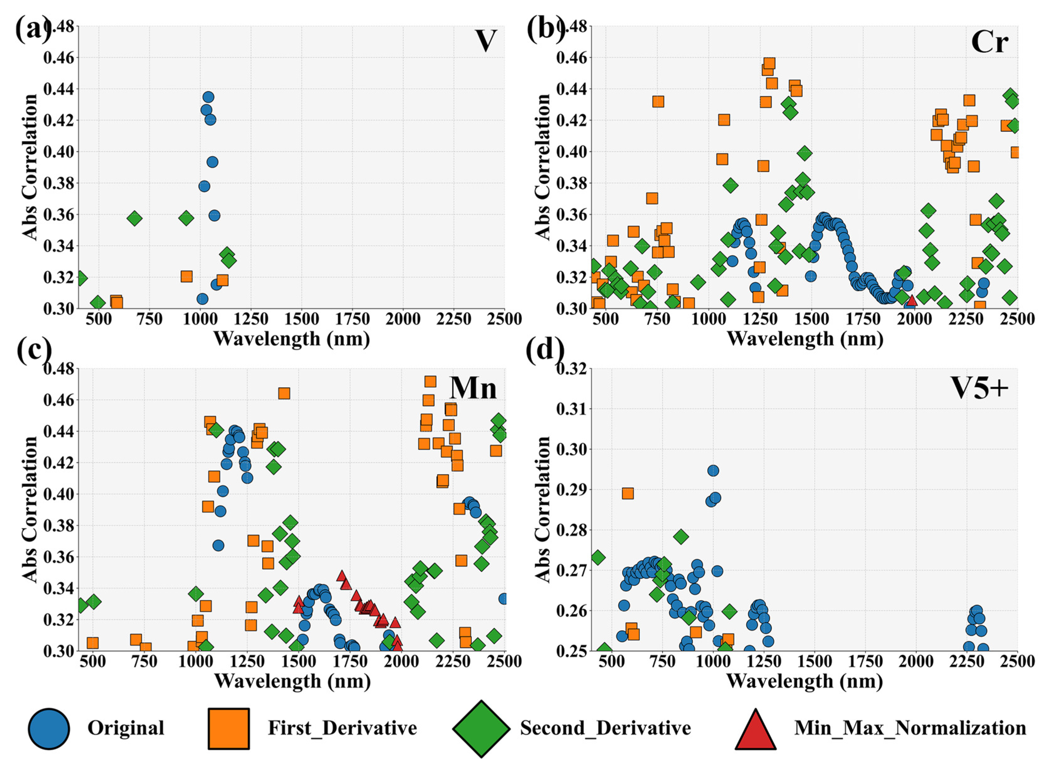
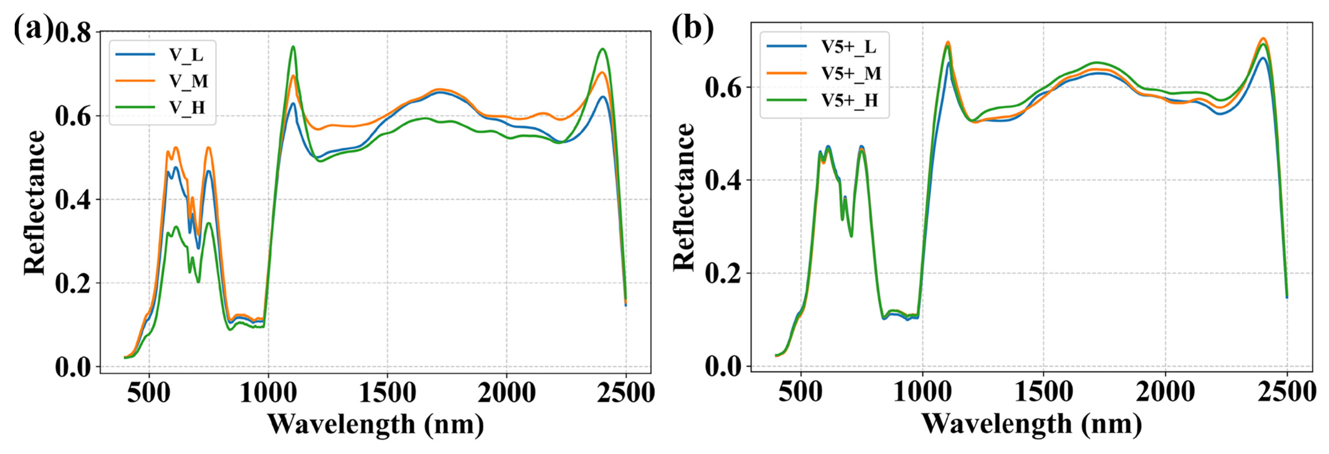
3.1.2. Spectral Feature Extraction

Figure 5 shows the distribution of characteristic bands for V and V5+ under different spectral preprocessing methods, as well as an analysis of their associated elements (Cr and Mn). Figure 5a shows that the spectral features of V are concentrated in the 400–1150 nm range, with absolute correlation coefficients between 0.3 and 0.44. The 930–1150 nm range shows higher and more continuous correlation coefficients corresponding to the absorption peaks of Fe²⁺ and Mn [22]. In comparison, Figure 5b,c show the spectral feature distributions of Cr and Mn. V shows weaker absolute correlation coefficients and narrower reflectance band ranges compared to Cr and Mn, suggesting the possibility of using the spectral features of Cr and Mn to indirectly predict V content. Figure 5d shows the spectral feature distribution of V5+ under different preprocessing methods. The spectral features of V5+ are mainly concentrated in the 500–1260 nm range. Compared to V, the spectral features of V5+ are weaker, with absolute correlation coefficients ranging from 0.25 to 0.31. In addition, a pronounced absorption peak near 2250 nm is observed, which is probably related to the binding of V5+ to groups such as hydroxyl (OH), ammonium (NH₄⁺), and carbonate (CO₃²⁻). These interactions between functional groups and metal cations can cause spectral features to shift to longer wavelengths [73].

Based on the spectral characteristic distribution of V and V5+, we further explain the spectral curve behavior of V and V5+ at different concentrations (Figure 6) by calculating the percentiles of the element content. For V (Figure 6a), reflectance rises with increasing concentration, peaking at 930–1150 nm with significant variation at 400–700 nm, and exhibits peaks at 550 nm and 900–1000 nm in the near-infrared range, consistent with Figure 5a. In contrast, for V5+ (Figure 6b), reflectance shows a modest increase at 500–1260 nm, with lower variability compared to V, and enhanced absorption at 2250 nm at higher concentrations, consistent with Figure 5d.

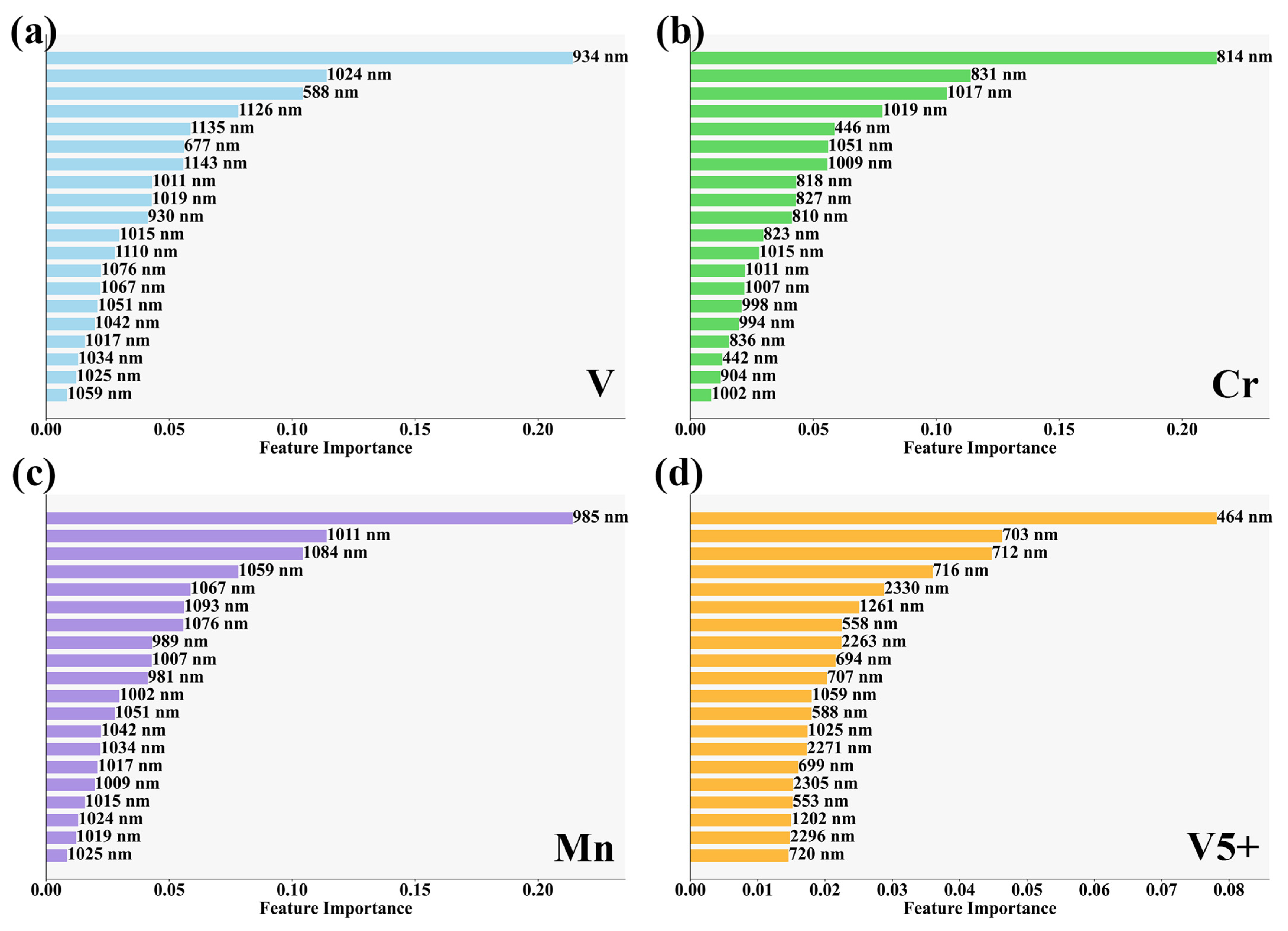
3.1.3. Performance of Characteristic Band Importance

After the processes of feature band extraction and spectral index construction, the spectral characteristics of vanadium (V) and its associated elements chromium (Cr), manganese (Mn), and pentavalent vanadium (V5+) were identified, enabling the extraction of the corresponding bands from the GF-5B satellite data. These bands were then subjected to an importance ranking concerning the measured concentrations of V and V5+ obtained during sampling (Figure 7). For V, Cr, and Mn, single significant bands with importance scores greater than 0.2 were identified at 934 nm, 814 nm, and 985 nm, respectively. These wavelengths are in the shortwave infrared (SWIR) region, although their response characteristics differ significantly. The characteristic bands of V5+, on the other hand, have a more uniform importance distribution, with a significant band at 464 nm (importance score of 0.08) located in the blue light region. In terms of wavelength distribution, the characteristic bands of V and Mn are mainly concentrated in the SWIR region, while Cr and V5+ cover a broader spectrum.

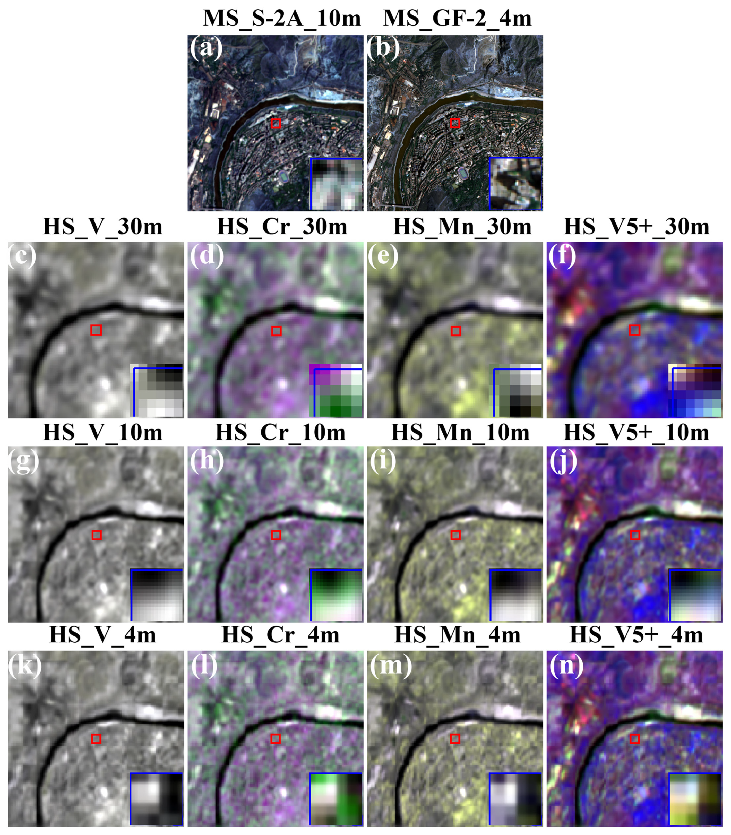
3.2. Performance of Image Fusion

The quantitative evaluation of image fusion models combining GF-5B with Sentinel-2A and GF-2 (

Table 5. Quantitative evaluation of the image fusion models for HS and MS.

Model (S-2A)	PSNR (db)	SSIM	FSIM	Model (GF-2)	PSNR (db)	SSIM	FSIM
${\mathrm{V}}_{\mathrm{s}}$	31.253	0.946	0.964	${\mathrm{V}}_{\mathrm{s}}$	31.066	0.937	0.952
$\mathrm{C}{\mathrm{r}}_{\mathrm{S}}$	30.377	0.937	0.955	$\mathrm{C}{\mathrm{r}}_{\mathrm{S}}$	29.517	0.924	0.947
$\mathrm{M}{\mathrm{n}}_{\mathrm{S}}$	30.534	0.949	0.957	$\mathrm{M}{\mathrm{n}}_{\mathrm{S}}$	29.870	0.938	0.953
$\mathrm{V}5{+}_{\mathrm{S}}$	32.307	0.957	0.969	$\mathrm{V}5{+}_{\mathrm{S}}$	31.363	0.953	0.949

Specifically, ${\mathrm{V}}_{\mathrm{s}}$, $\mathrm{C}{\mathrm{r}}_{\mathrm{S}}$, $\mathrm{M}{\mathrm{n}}_{\mathrm{S}}$ and $\mathrm{V}5{+}_{\mathrm{S}}$ represent the characteristic bands of their corresponding elements.

) reveals that the fusion performance of characteristic bands for different elements follows the order: V5+ > V > Cr > Mn. However, as the spatial resolution differences between the fused images increase, the fusion performance tends to degrade. Consequently, the spectral details of the HS images may be slightly distorted due to the influence of high-resolution images. Nevertheless, the DB-CNN model demonstrates robust spectral fidelity across different scales during the fusion process. Figure 8 presents the fusion results of GF-5B with Sentinel-2A and GF-2. By comparing the input MS and HS characteristic band images at different scales (4 m, 10 m, and 30 m) with the fused images, it is evident that the fused HS images effectively capture the spatial details of the MS images. This is reflected in improved edge sharpness and reduced noise. The results indicate that the DB-CNN model demonstrates good efficacy in integrating spatial details with spectral information.

3.3. Model Construction

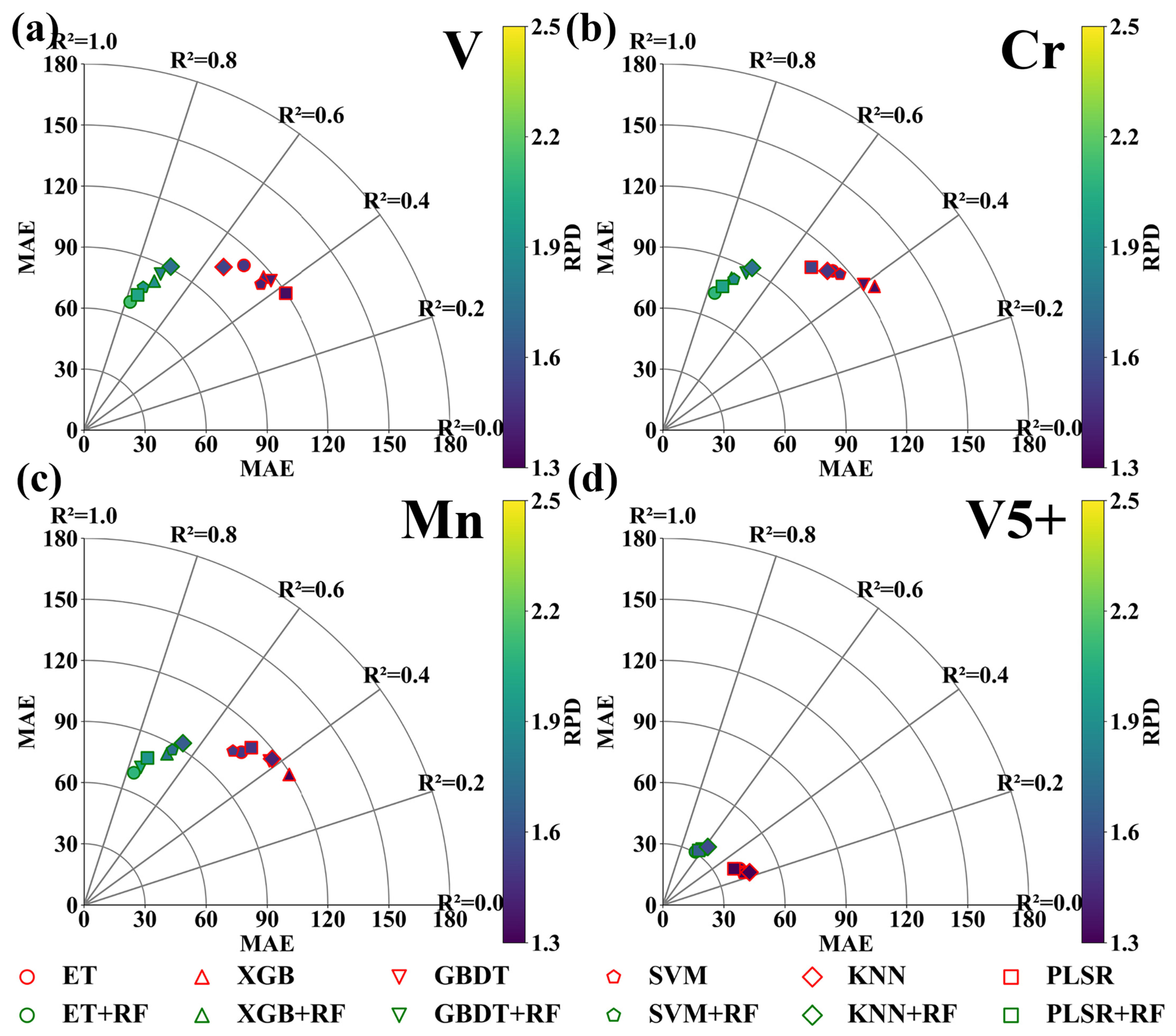
3.3.1. Traditional Machine Learning Models

Table 6. Prediction results of the basic models for V, Cr, Mn, and V5+, evaluated using the coefficient of determination (R²), ratio of performance to deviation (RPD), and mean absolute error (MAE).

Element	Metric	ET	XGB	GBDT	SVM	KNN	PLSR
	R2	0.51	0.45	0.43	0.44	0.38	0.54
V	RPD	1.49	1.43	1.39	1.41	1.34	1.54
	MAE	112.83	115.91	117.6	112.63	119.82	105.51
	R2	0.48	0.38	0.4	0.46	0.53	0.49
Cr	RPD	1.46	1.34	1.36	1.45	1.53	1.48
	MAE	114.37	125.76	121.84	115.94	108.28	112.53
	R2	0.49	0.36	0.42	0.51	0.48	0.42
Mn	RPD	1.49	1.3	1.37	1.5	1.48	1.41
	MAE	107.59	119.36	115.25	105.09	112.62	116.84
	R2	0.28	0.29	0.25	0.24	0.3	0.23
V5+	RPD	1.27	1.28	1.24	1.23	1.29	1.21
	MAE	41.82	40.69	41.95	42.24	39.16	45.54

compares the performance of six basic models in predicting the elements V, V5+, and their highly correlated elements (Cr, Mn), using R² as the evaluation metric. The results are as follows: V: PLSR > ET > SVM > XGB > GBDT > KNN; Cr: KNN > PLSR > ET > SVM > GBDT > XGB; Mn: SVM > ET > KNN > PLSR > GBDT > XGB; V5+: KNN > XGB > ET > SVM > GBDT > PLSR. PLSR shows somewhat better performance in predicting V (R² = 0.54), while KNN tends to perform somewhat better in predicting Cr and V5+ (R² = 0.53 and 0.3, respectively). The SVM shows a modest advantage in predicting Mn (R² = 0.51). When comparing indirect predictions of V content using the characteristic bands of Cr and Mn with direct predictions, the latter yielded better results (R²: 0.54 > 0.53 > 0.51).

However, the R² values of these basic models, ranging from 0.3 to 0.54, indicate limited predictive capability, only marginally meeting the threshold for practical prediction. In the case of V5+, although each model showed lower MAE values compared to V, the basic models were almost unable to accurately predict its content (R² ≤ 0.3), which can be attributed to the weak spectral correlation of V5+ [74]. These results suggest that the overall modeling accuracy of traditional machine learning methods remains relatively poor, and these models need to be optimized to improve prediction accuracy.

3.3.2. Optimized Random Forest Model

Figure 9 compares the evaluation results of the optimized random forest model after reducing prediction errors for the basic models in predicting V, V5+, and their highly correlated elements (Cr, Mn). Compared to the basic models, the optimized models demonstrate better prediction accuracy, achieving good performance with R² values exceeding 0.7 for V, Cr, and Mn, while the R² value for V5+ exceeds 0.6, indicating moderate prediction accuracy. Compared to the basic models, the differences in evaluation metrics among the optimized models become more stable.

Within the optimized random forest model combinations, the best-performing model was the ET + RF combination. This model achieved an R² of 0.79 for the direct prediction of V, outperforming predictions for Cr (R² = 0.77) and Mn (R² = 0.76), while the R² for V5+ improved to 0.66. These results indicate that the optimized random forest model can effectively predict the V5+ content even in cases of weak spectral correlations. Moreover, the indirect prediction method failed to improve the prediction accuracy for V. Therefore, in subsequent multi-scale analyses, we employed only the optimized random forest model to predict V and V5+.

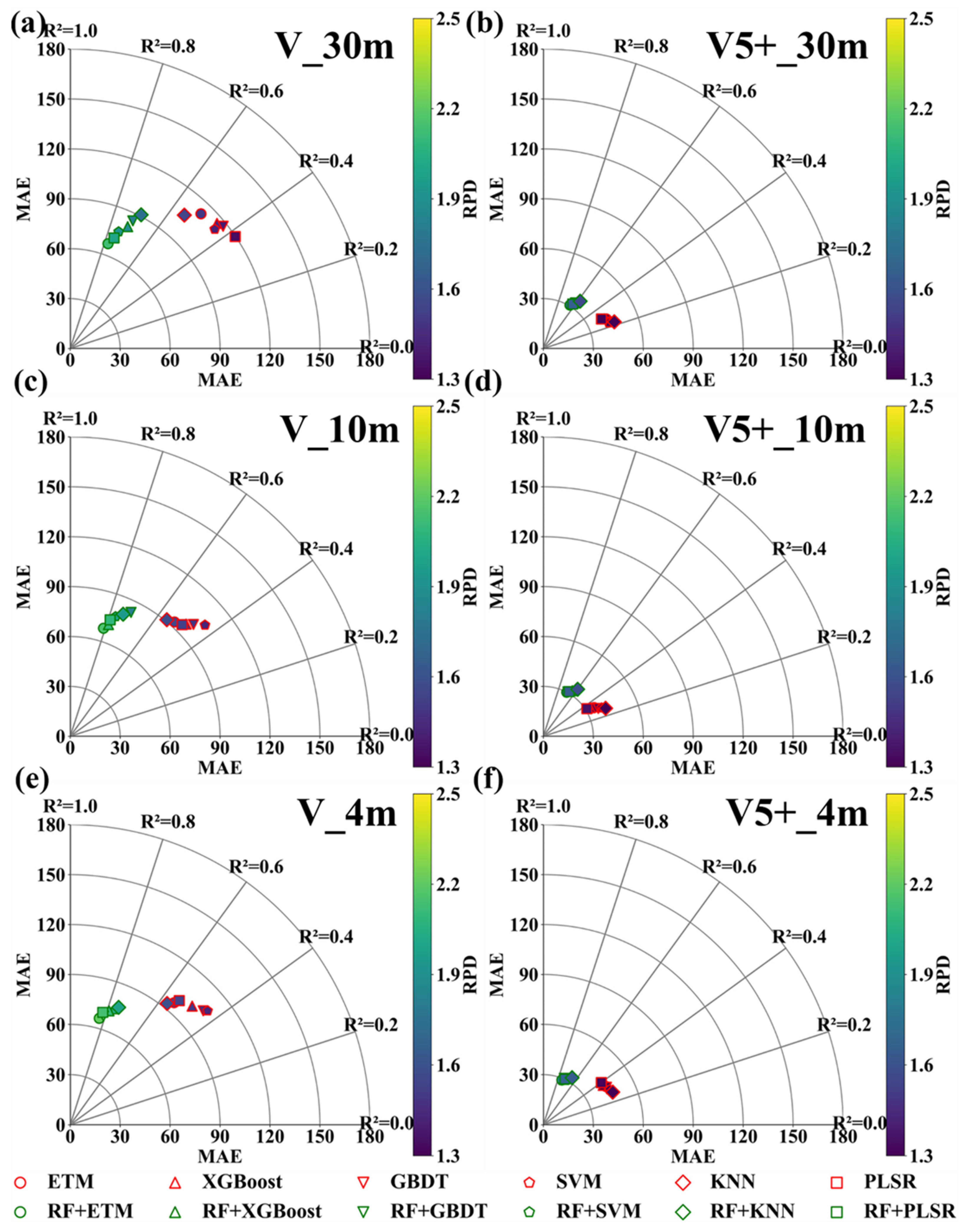
3.3.3. Random Forest Optimization Model Based on Image Fusion

Figure 10 presents the evaluation results of the optimized random forest model for predicting V and V5+ in the experimental and control groups. The optimal base models and random forest combinations remained consistent across all groups (V: PLSR, ET + RF; V5+: KNN, ET + RF). For V, the R² values improved by 54.90%, 52.83%, and 53.70%, while for V5+, the R² values increased by 135.71%, 109.09%, and 114.29%, respectively. These results demonstrate the stability and reliability of the optimized random forest model in enhancing prediction accuracy.

To comprehensively assess the improvement in prediction accuracy achieved by the ET + RF model, scatter plots were generated using both the training and validation datasets, as shown in Figure 11. As the spatial resolution increased from 30 m to 10 m and 4 m, the R² for V predicted by the ET + RF combination improved from 0.79 to 0.81 and 0.83, respectively, while for V5+, the R² increased from 0.66 to 0.69 and 0.75, respectively. The model performed well over most of the content ranges, although slight deviations from the 1:1 line were observed near the extreme values, with low values overestimated and high values underestimated. This phenomenon is related to the right-skewed distribution of V and V5+. Among the experimental and control groups, the 4 m scale exhibited the best prediction performance. Therefore, in subsequent experiments, we selected only the feature bands for V and V5+ at the 4 m scale and used the ET + RF model for spatial distribution prediction.

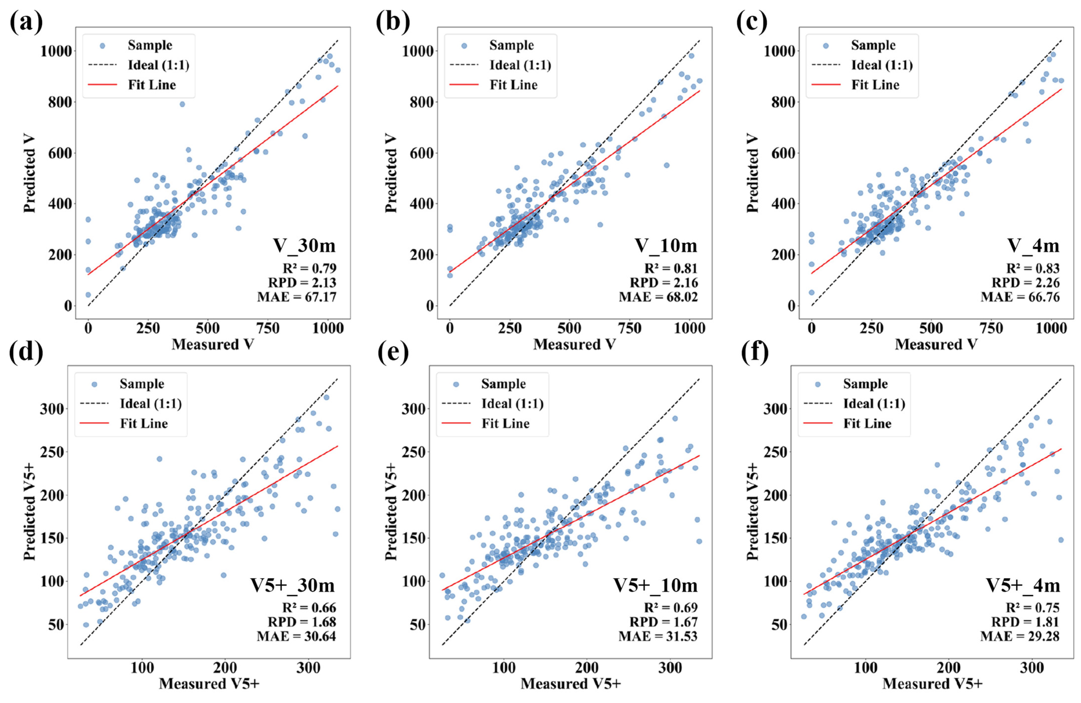
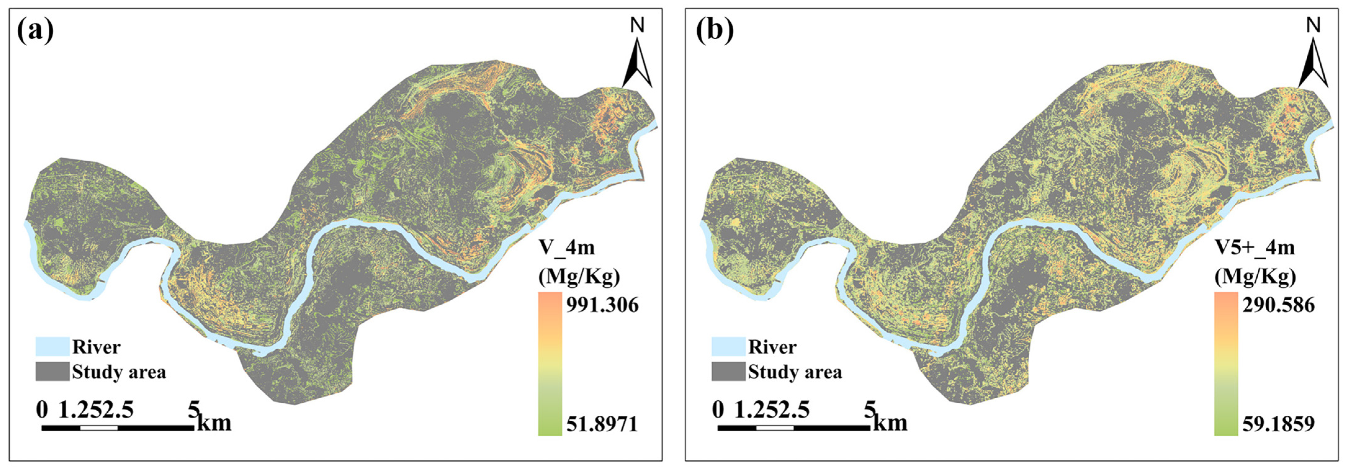
3.4. Soil Vanadium Concentration Map

Based on the ET + RF integrated model, the predicted results for V and V5+ at a 4 m scale are shown in Figure 12. The content distribution ranges for V and V5+ in the study area are 991.31–51.90 (mg/kg) and 290.59–59.19 (mg/kg), respectively, indicating significant V contamination in the area. V is primarily concentrated in the mining and smelting regions, with high values exhibiting a clustered and banded distribution pattern, reflecting strong spatial heterogeneity. V5+ is mainly concentrated in the mining area, although some V and V5+ accumulation is also observed on the southern bank of the river, despite both the mining and smelting areas being located on the northern bank. This phenomenon may be related to the transport of materials by the prevailing wind [75].

4. Discussion

Accurate monitoring of vanadium contamination in soil is crucial for ecological protection and public health. This study employs a DB-CNN method that fuses HS and MS data, combined with RF optimization, to reduce prediction errors and identify the optimal model combination. The results show that both image fusion and random forest optimization significantly improve the model’s predictive accuracy. Image fusion allows HS data to capture the spatial information from MS images, thereby improving pixel purity. Despite the potential benefits of image fusion, the DB-CNN method is efficient and eliminates the need to address band correspondence, making it suitable for regression tasks. The random forest model captures nonlinear relationships through error correction, optimizing the selection of splitting points in the ET model, thus improving prediction accuracy. Despite the lack of interpretability in the ET + RF model and the absence of clear parameters, the ET + RF combination demonstrates strong predictive capability, especially for components with unknown spectral properties and varying oxidation states. This model is therefore recommended for future predictions.

The aggregation and symbiotic interactions among elements are crucial for exploring the concentrations of unidentified elements [21,76]. The correlation between element concentrations can reflect their similarity in geochemical characteristics [53], but the effectiveness of indirect predictions primarily depends on the spectral coupling of target elements with their associated components at critical absorption wavelengths [77]. Pearson correlation analysis reveals that vanadium (V) has the strongest association with chromium (Cr) and manganese (Mn). Despite Cr and Mn exhibiting strong reflective properties and broad spectral coverage, band significance analysis indicates that the key features critical for predicting V and V5+ are confined to a small number of specific bands. The bands at 934 nm and 464 nm account for 22% and 8% of the relative importance, respectively, and they differ from the characteristic bands of Cr and Mn. As a result, this study demonstrates that direct prediction based on the distinctive absorption peaks of V and V5+ yields higher accuracy. While the correlation with iron (Fe) is lower, prior research has shown that Fe’s characteristic bands primarily fall between 860 and 930 nm, aligning with the symbiotic relationship of V-Ti-Fe minerals, such as vanadiferous titanomagnetite and vanadiferous hematite [78,79,80]. Future research should integrate correlation analysis among elements and between elements and spectra for indirect predictions to improve model accuracy.

HS data often exhibit high spectral sampling intervals but lower spatial resolution, while image fusion can overcome the limitation of the “trade-off between spectral and spatial resolution” by integrating spatial information from MS data. The DB-CNN method enables rapid and efficient image fusion, achieving fusion times under 5 min while maintaining strong performance in terms of signal-to-noise ratio, structural integrity, and feature preservation (PSNR > 30, SSIM, FSIM > 90), making it suitable for regression tasks. The fusion results enhance pixel purity, facilitating the capture of bare soil characteristics [81], which in turn improves prediction accuracy and provides strong support for monitoring vanadium (V) and V5+ contamination at fine spatial resolutions. Furthermore, when the spatial resolution of HS and MS data is comparable, the fusion outcomes are significantly enhanced [33]. This study found that when the spatial resolution was increased from 10 m to 4 m, the average PSNR, SSIM, and FSIM decreased by 2.13%, 0.98%, and 1.14%, respectively. Nevertheless, the fused image retained additional information, leading to an improvement in modeling accuracy of 3.57% for V and 8.33% for V5+. Future research can further explore the synergistic information between HS and MS data and select appropriate fusion combinations to meet the demands of high-precision predictions [82].

In this study, there is no universally optimal base model for all scenarios, and the prediction accuracy of the base models still has room for improvement, with the R² of the optimal base model being only 0.55. Among the base models, non-decision tree models achieved the best predictive performance, taking advantage of flexible parameter tuning and adaptability to nonlinear relationships, resulting in smoother mappings [83]. However, traditional boosting methods, such as XGBoost and GBDT, improve performance by iteratively correcting the errors of base learners of the same type, but they still face limitations related to overfitting and spatial autocorrelation [84,85]. Meanwhile, stacking algorithms in ensemble learning can improve performance by combining different models, but they still run the risk of base model performance limitations and error accumulation [28,86]. When the correlation between models is too high, stacking methods have difficulty achieving complementary advantages between models [87]. The random forest optimization method proposed in this study integrates the concepts of boosting algorithms and gradually optimizes the prediction errors of different base models by adjusting the learning rate α. The ET + RF combination was selected as the optimal model, avoiding error accumulation. At different scales, the average prediction accuracy for V and V5+ increased by 53.81% and 119.70%, respectively. Future research can further explore the combination of different machine learning models and optimization techniques to improve model prediction accuracy and stability.

In addition, there remain some limitations in this study. Although image fusion and bare soil extraction have improved pixel purity, the mixed pixel issue is not completely resolved, indicating that more refined fusion methods or unmixing techniques are required to further enhance accuracy [88]. Moreover, the limited interpretability of DB-CNN and ET + RF impedes a comprehensive understanding of the models’ internal mechanisms [40], leaving room for further improvement in prediction accuracy [89]. In view of these challenges, future research should focus on developing more advanced model-building approaches to improve predictive performance while also exploring interpretable modeling methods to clarify the internal mechanisms of complex models. Subsequently, efforts should be directed toward investigating additional elements, such as radioactive elements and hexavalent chromium, which suffer from insufficient spectral data or variable oxidation states and have significant impacts on human health. Furthermore, extending these methods to track heavy metals in mid-scale complex landscapes could enhance their applicability and contribute to more effective environmental monitoring.

5. Conclusions

Comprehensive monitoring of vanadium pollution is essential for assessing ecological and health risks. This study employs a DB-CNN approach for the fusion of HS images, combined with RF optimization to reduce machine learning prediction errors and identify the optimal model combination. The results demonstrate that both image fusion and random forest optimization significantly improve the model’s predictive accuracy. Image fusion enables HS data to capture the spatial information of MS images, thereby enhancing pixel purity. While there is potential for further performance improvement, the DB-CNN method is efficient and eliminates the need to consider band correspondence, making it suitable for regression tasks. The RF captures nonlinear characteristics through error correction, optimizing the selection of split points in the ET model, thus improving prediction accuracy. Despite the ET + RF model being a black-box system with non-interpretable parameters, its integrated approach demonstrates robust predictive capability, especially in identifying elements with limited spectral characterization (for example, V) and those with fluctuating oxidation states (for example, V5+). Future research is encouraged to apply image fusion for tracking heavy metals in mid-scale complex landscapes. The enhanced random forest approach may also be extended to explore additional elements, such as radioactive elements and hexavalent chromium, which have insufficient spectral data or variable oxidation states and significantly impact human health.

References

1. Islam, S.; Ahmed, K.; Habibullah-Al-Mamun; Masunaga, S. Potential Ecological Risk of Hazardous Elements in Different Land-Use Urban Soils of Bangladesh. Sci. Total Environ. 2015, 512–513, 94–102. [Google Scholar] [CrossRef] [PubMed]
2. Adnan, M.; Xiao, B.; Ali, M.U.; Xiao, P.; Zhao, P.; Wang, H.; Bibi, S. Heavy Metals Pollution from Smelting Activities: A Threat to Soil and Groundwater. Ecotoxicol. Environ. Saf. 2024, 274, 116189. [Google Scholar] [CrossRef] [PubMed]
3. Schlesinger, W.H.; Klein, E.M.; Vengosh, A. Global Biogeochemical Cycle of Vanadium. Proc. Natl. Acad. Sci. USA 2017, 114, E11092–E11100. [Google Scholar] [CrossRef] [PubMed]
4. Tang, X.; Huang, Y.; Li, Y.; Yang, Y.; Cheng, X.; Jiao, G.; Dai, H. The Response of Bacterial Communities to V and Cr and Novel Reducing Bacteria near a Vanadium-titanium Magnetite Refinery. Sci. Total Environ. 2022, 806, 151214. [Google Scholar] [CrossRef]
5. Gan, C.; Yang, J.; Li, J.; Yang, M.; Du, X.; Nikitin, A. Transcriptome Analysis Reveals Vanadium Reduction Mechanisms in a Bacterium of Pseudomonas Balearica. J. Clean. Prod. 2024, 454, 142258. [Google Scholar] [CrossRef]
6. Cheng, M.; Yin, X.; Zhang, H. Insights into the Hydrogen-Fueled Bioreduction of Vanadium(V) by Marine Shewanella Sp. FDA-1: Process and Mechanism. J. Hazard. Mater. 2025, 483, 136585. [Google Scholar] [CrossRef]
7. Cao, X.; Diao, M.; Zhang, B.; Liu, H.; Wang, S.; Yang, M. Spatial Distribution of Vanadium and Microbial Community Responses in Surface Soil of Panzhihua Mining and Smelting Area, China. Chemosphere 2017, 183, 9–17. [Google Scholar] [CrossRef]
8. Li, Y.; Zhang, B.; Liu, Z.; Wang, S.; Yao, J.; Borthwick, A.G.L. Vanadium Contamination and Associated Health Risk of Farmland Soil near Smelters throughout China. Environ. Pollut. 2020, 263, 114540. [Google Scholar] [CrossRef]
9. Ścibior, A.; Wnuk, E.; Gołębiowska, D. Wild Animals in Studies on Vanadium Bioaccumulation—Potential Animal Models of Environmental Vanadium Contamination: A Comprehensive Overview with a Polish Accent. Sci. Total Environ. 2021, 785, 147205. [Google Scholar] [CrossRef]
10. Yang, N.; Han, L.; Liu, M. Inversion of Soil Heavy Metals in Metal Tailings Area Based on Different Spectral Transformation and Modeling Methods. Heliyon 2023, 9, e19782. [Google Scholar] [CrossRef]
11. Gholizadeh, A.; Saberioon, M.; Ben-Dor, E.; Borůvka, L. Monitoring of Selected Soil Contaminants Using Proximal and Remote Sensing Techniques: Background, State-of-the-Art and Future Perspectives. Crit. Rev. Environ. Sci. Technol. 2018, 48, 243–278. [Google Scholar] [CrossRef]
12. Shi, T.; Liu, H.; Chen, Y.; Wang, J.; Wu, G. Estimation of Arsenic in Agricultural Soils Using Hyperspectral Vegetation Indices of Rice. J. Hazard. Mater. 2016, 308, 243–252. [Google Scholar] [CrossRef] [PubMed]
13. Zeraatpisheh, M.; Ayoubi, S.; Jafari, A.; Tajik, S.; Finke, P. Digital Mapping of Soil Properties Using Multiple Machine Learning in a Semi-Arid Region, Central Iran. Geoderma 2019, 338, 445–452. [Google Scholar] [CrossRef]
14. Xie, Y.; Chen, T.; Lei, M.; Yang, J.; Guo, Q.; Song, B.; Zhou, X. Spatial Distribution of Soil Heavy Metal Pollution Estimated by Different Interpolation Methods: Accuracy and Uncertainty Analysis. Chemosphere 2011, 82, 468–476. [Google Scholar] [CrossRef] [PubMed]
15. Shi, T.; Guo, L.; Chen, Y.; Wang, W.; Shi, Z.; Li, Q.; Wu, G. Proximal and Remote Sensing Techniques for Mapping of Soil Contamination with Heavy Metals. Appl. Spectrosc. Rev. 2018, 53, 783–805. [Google Scholar] [CrossRef]
16. Zahra, A.; Qureshi, R.; Sajjad, M.; Sadak, F.; Nawaz, M.; Khan, H.A.; Uzair, M. Current Advances in Imaging Spectroscopy and Its State-of-the-Art Applications. Expert Syst. Appl. 2024, 238, 122172. [Google Scholar] [CrossRef]
17. Song, Y.; Sun, N.; Zhang, L.; Wang, L.; Su, H.; Chen, Z.; Yu, H.; Li, B. Using Multispectral Variables to Estimate Heavy Metals Content in Agricultural Soils: A Case of Suburban Area in Tianjin, China. Geoderma Reg. 2022, 29, e00540. [Google Scholar] [CrossRef]
18. Sun, Y.; Chen, S.; Dai, X.; Li, D.; Jiang, H.; Jia, K. Coupled Retrieval of Heavy Metal Nickel Concentration in Agricultural Soil from Spaceborne Hyperspectral Imagery. J. Hazard. Mater. 2023, 446, 130722. [Google Scholar] [CrossRef]
19. Tan, K.; Wang, H.; Chen, L.; Du, Q.; Du, P.; Pan, C. Estimation of the Spatial Distribution of Heavy Metal in Agricultural Soils Using Airborne Hyperspectral Imaging and Random Forest. J. Hazard. Mater. 2020, 382, 120987. [Google Scholar] [CrossRef]
20. Wang, J.; Hu, X.; Shi, T.; He, L.; Hu, W.; Wu, G. Assessing Toxic Metal Chromium in the Soil in Coal Mining Areas via Proximal Sensing: Prerequisites for Land Rehabilitation and Sustainable Development. Geoderma 2022, 405, 115399. [Google Scholar] [CrossRef]
21. Wang, F.; Gao, J.; Zha, Y. Hyperspectral Sensing of Heavy Metals in Soil and Vegetation: Feasibility and Challenges. ISPRS J. Photogramm. Remote Sens. 2018, 136, 73–84. [Google Scholar] [CrossRef]
22. Shi, T.; Chen, Y.; Liu, Y.; Wu, G. Visible and Near-Infrared Reflectance Spectroscopy—An Alternative for Monitoring Soil Contamination by Heavy Metals. J. Hazard. Mater. 2014, 265, 166–176. [Google Scholar] [CrossRef] [PubMed]
23. Laparrcr, V.; Santos-Rodriguez, R. Spatial/Spectral Information Trade-off in Hyperspectral Images. In Proceedings of the 2015 IEEE International Geoscience and Remote Sensing Symposium (IGARSS), Milan, Italy, 26–31 July 2015; pp. 1124–1127. [Google Scholar]
24. Bhargava, A.; Sachdeva, A.; Sharma, K.; Alsharif, M.H.; Uthansakul, P.; Uthansakul, M. Hyperspectral Imaging and Its Applications: A Review. Heliyon 2024, 10, e33208. [Google Scholar] [CrossRef]
25. Wang, Y.; Zhang, X.; Sun, W.; Wang, J.; Ding, S.; Liu, S. Effects of Hyperspectral Data with Different Spectral Resolutions on the Estimation of Soil Heavy Metal Content: From Ground-Based and Airborne Data to Satellite-Simulated Data. Sci. Total Environ. 2022, 838, 156129. [Google Scholar] [CrossRef] [PubMed]
26. Yao, L.; Xu, M.; Liu, Y.; Niu, R.; Wu, X.; Song, Y. Estimating of Heavy Metal Concentration in Agricultural Soils from Hyperspectral Satellite Sensor Imagery: Considering the Sources and Migration Pathways of Pollutants. Ecol. Indic. 2024, 158, 111416. [Google Scholar] [CrossRef]
27. Melser, R.; Coops, N.C.; Wulder, M.A.; Derksen, C. Multi-Source Remote Sensing Based Modeling of Vegetation Productivity in the Boreal: Issues & Opportunities. Can. J. Remote Sens. 2023, 49, 2256895. [Google Scholar] [CrossRef]
28. Zhou, Y.; Liu, C.; Wang, J.; Zhang, M.-W.; Wang, X.; Zeng, L.-T.; Cui, Y.-P.; Wang, H.; Sun, X.-L. Monitoring Soil Arsenic Content in Densely Vegetated Agricultural Areas Using UAV Hyperspectral, Satellite Multispectral and SAR Data. J. Hazard. Mater. 2025, 484, 136689. [Google Scholar] [CrossRef]
29. Sara, D.; Mandava, A.K.; Kumar, A.; Duela, S.; Jude, A. Hyperspectral and Multispectral Image Fusion Techniques for High Resolution Applications: A Review. Earth Sci. Inform. 2021, 14, 1685–1705. [Google Scholar] [CrossRef]
30. Allu, A.R.; Mesapam, S. Impact of Remote Sensing Data Fusion on Agriculture Applications: A Review. Eur. J. Agron. 2025, 164, 127478. [Google Scholar] [CrossRef]
31. Song, W.; Li, S.; Fang, L.; Lu, T. Hyperspectral Image Classification With Deep Feature Fusion Network. IEEE Trans. Geosci. Remote Sens. 2018, 56, 3173–3184. [Google Scholar] [CrossRef]
32. Vivone, G. Multispectral and Hyperspectral Image Fusion in Remote Sensing: A Survey. Inf. Fusion 2023, 89, 405–417. [Google Scholar] [CrossRef]
33. Dian, R.; Li, S.; Sun, B.; Guo, A. Recent Advances and New Guidelines on Hyperspectral and Multispectral Image Fusion. Inf. Fusion 2021, 69, 40–51. [Google Scholar] [CrossRef]
34. Yang, J.; Zhao, Y.-Q.; Chan, J.C.-W. Hyperspectral and Multispectral Image Fusion via Deep Two-Branches Convolutional Neural Network. Remote Sens. 2018, 10, 800. [Google Scholar] [CrossRef]
35. Laszlo, E.; Szolgay, P.; Nagy, Z. Analysis of a GPU Based CNN Implementation. In Proceedings of the 2012 13th International Workshop on Cellular Nanoscale Networks and their Applications, Turin, Italy, 29–31 August 2012; pp. 1–5. [Google Scholar]
36. Nkinahamira, F.; Feng, A.; Zhang, L.; Rong, H.; Ndagijimana, P.; Guo, D.; Cui, B.; Zhang, H. Machine Learning Approaches for Monitoring Environmental Metal Pollutants: Recent Advances in Source Apportionment, Detection, Quantification, and Risk Assessment. TrAC Trends Anal. Chem. 2024, 180, 117980. [Google Scholar] [CrossRef]
37. Lovynska, V.; Bayat, B.; Bol, R.; Moradi, S.; Rahmati, M.; Raj, R.; Sytnyk, S.; Wiche, O.; Wu, B.; Montzka, C. Monitoring Heavy Metals and Metalloids in Soils and Vegetation by Remote Sensing: A Review. Remote Sens. 2024, 16, 3221. [Google Scholar] [CrossRef]
38. Koldasbayeva, D.; Tregubova, P.; Gasanov, M.; Zaytsev, A.; Petrovskaia, A.; Burnaev, E. Challenges in Data-Driven Geospatial Modeling for Environmental Research and Practice. Nat. Commun. 2024, 15, 10700. [Google Scholar] [CrossRef]
39. Al-Shboul, K.F. Unraveling the Complex Interplay between Soil Characteristics and Radon Surface Exhalation Rates through Machine Learning Models and Multivariate Analysis. Environ. Pollut. 2023, 336, 122440. [Google Scholar] [CrossRef]
40. Zou, Z.; Wang, Q.; Wu, Q.; Li, M.; Zhen, J.; Yuan, D.; Zhou, M.; Xu, C.; Wang, Y.; Zhao, Y.; et al. Inversion of Heavy Metal Content in Soil Using Hyperspectral Characteristic Bands-Based Machine Learning Method. J. Environ. Manag. 2024, 355, 120503. [Google Scholar] [CrossRef]
41. Zhang, Y.; Liu, J.; Shen, W. A Review of Ensemble Learning Algorithms Used in Remote Sensing Applications. Appl. Sci. 2022, 12, 8654. [Google Scholar] [CrossRef]
42. Khan, Z.; Gul, A.; Perperoglou, A.; Miftahuddin, M.; Mahmoud, O.; Adler, W.; Lausen, B. Ensemble of Optimal Trees, Random Forest and Random Projection Ensemble Classification. Adv. Data Anal. Classif. 2020, 14, 97–116. [Google Scholar] [CrossRef]
43. Luo, Y.; Su, S. SpatioTemporal Random Forest and SpatioTemporal Stacking Tree: A Novel Spatially Explicit Ensemble Learning Approach to Modeling Non-Linearity in Spatiotemporal Non-Stationarity. Int. J. Appl. Earth Obs. Geoinf. 2025, 136, 104315. [Google Scholar] [CrossRef]
44. Gan, C.; Yang, J.; Liu, R.; Li, X.; Tang, Q. Contrasted Speciation Distribution of Toxic Metal(Loid)s and Microbial Community Structure in Vanadium-Titanium Magnetite Tailings under Dry and Wet Disposal Methods. J. Hazard. Mater. 2022, 439, 129624. [Google Scholar] [CrossRef] [PubMed]
45. HJ/T 166-2004; State Environmental Protection Administration of the People’s Republic of China Technical Specification for Soil Environmental Monitoring. State Environmental Protection Administration of the People’s Republic of China: Shenzhen, China, 2004.
46. Ma, X.; Wang, J.; Zhou, K.; Zhang, W.; Zhang, Z.; Zhou, S.; Bai, Y.; De Maeyer, P.; Van De Voorde, T. Quantitative Evaluation of the Impact of Band Optimization Methods on the Accuracy of the Hyperspectral Metal Element Inversion Models. Int. J. Appl. Earth Obs. Geoinf. 2024, 132, 104011. [Google Scholar] [CrossRef]
47. Liu, F.T.; Ting, K.M.; Zhou, Z.-H. Isolation Forest. In Proceedings of the 2008 Eighth IEEE International Conference on Data Mining, Pisa, Italy, 15–19 December 2008; pp. 413–422. [Google Scholar]
48. Zhang, B.; Guo, B.; Zou, B.; Wei, W.; Lei, Y.; Li, T. Retrieving Soil Heavy Metals Concentrations Based on GaoFen-5 Hyperspectral Satellite Image at an Opencast Coal Mine, Inner Mongolia, China. Environ. Pollut. 2022, 300, 118981. [Google Scholar] [CrossRef]
49. Ding, S.; Zhang, X.; Sun, W.; Shang, K.; Wang, Y. Estimation of Soil Lead Content Based on GF-5 Hyperspectral Images, Considering the Influence of Soil Environmental Factors. J. Soils Sediments 2022, 22, 1431–1445. [Google Scholar] [CrossRef]
50. Yin, F.; Wu, M.; Liu, L.; Zhu, Y.; Feng, J.; Yin, D.; Yin, C.; Yin, C. Predicting the Abundance of Copper in Soil Using Reflectance Spectroscopy and GF5 Hyperspectral Imagery. Int. J. Appl. Earth Obs. Geoinf. 2021, 102, 102420. [Google Scholar] [CrossRef]
51. He, Z.; Gao, L.; Liang, M.; Zeng, Z.-C. A Survey of Methane Point Source Emissions from Coal Mines in Shanxi Province of China Using AHSI on Board Gaofen-5B. Atmos. Meas. Tech. 2024, 17, 2937–2956. [Google Scholar] [CrossRef]
52. Ren, K.; Sun, W.; Meng, X.; Yang, G.; Du, Q. Fusing China GF-5 Hyperspectral Data with GF-1, GF-2 and Sentinel-2A Multispectral Data: Which Methods Should Be Used? Remote Sens. 2020, 12, 882. [Google Scholar] [CrossRef]
53. Shen, Q.; Xia, K.; Zhang, S.; Kong, C.; Hu, Q.; Yang, S. Hyperspectral Indirect Inversion of Heavy-Metal Copper in Reclaimed Soil of Iron Ore Area. Spectrochim. Acta Part A Mol. Biomol. Spectrosc. 2019, 222, 117191. [Google Scholar] [CrossRef]
54. Zeiler, M.D.; Fergus, R. Visualizing and Understanding Convolutional Networks. In Computer Vision—ECCV 2014; Fleet, D., Pajdla, T., Schiele, B., Tuytelaars, T., Eds.; Lecture Notes in Computer Science; Springer International Publishing: Cham, Switzerland, 2014; Volume 8689, pp. 818–833. ISBN 978-3-319-10589-5. [Google Scholar]
55. Vasanthakumari, R.K.; Nair, R.V.; Krishnappa, V.G. Improved Learning by Using a Modified Activation Function of a Convolutional Neural Network in Multi-Spectral Image Classification. Mach. Learn. Appl. 2023, 14, 100502. [Google Scholar] [CrossRef]
56. Wang, X.; Wang, X.; Zhao, K.; Zhao, X.; Song, C. FSL-Unet: Full-Scale Linked Unet With Spatial–Spectral Joint Perceptual Attention for Hyperspectral and Multispectral Image Fusion. IEEE Trans. Geosci. Remote Sens. 2022, 60, 1–14. [Google Scholar] [CrossRef]
57. Wu, H.; Gui, J.; Xu, Y.; Wu, Z.; Tang, Y.Y.; Wei, Z. An Efficient Cross-Modality Self-Calibrated Network for Hyperspectral and Multispectral Image Fusion. IEEE Trans. Geosci. Remote Sens. 2022, 60, 1–12. [Google Scholar] [CrossRef]
58. Kalamkar, S.; Geetha, M.A. Multimodal Image Fusion: A Systematic Review. Decis. Anal. J. 2023, 9, 100327. [Google Scholar] [CrossRef]
59. Gelvez-Barrera, T.; Arguello, H.; Foi, A. Joint Nonlocal, Spectral, and Similarity Low-Rank Priors for Hyperspectral–Multispectral Image Fusion. IEEE Trans. Geosci. Remote Sens. 2022, 60, 1–12. [Google Scholar] [CrossRef]
60. Xie, Q.; Zhou, M.; Zhao, Q.; Xu, Z.; Meng, D. MHF-Net: An Interpretable Deep Network for Multispectral and Hyperspectral Image Fusion. IEEE Trans. Pattern Anal. Mach. Intell. 2022, 44, 1457–1473. [Google Scholar] [CrossRef]
61. Huang, S.; Tang, L.; Hupy, J.P.; Wang, Y.; Shao, G. A Commentary Review on the Use of Normalized Difference Vegetation Index (NDVI) in the Era of Popular Remote Sensing. J. For. Res. 2021, 32, 1–6. [Google Scholar] [CrossRef]
62. Jia, X.; Hou, D. Mapping Soil Arsenic Pollution at a Brownfield Site Using Satellite Hyperspectral Imagery and Machine Learning. Sci. Total Environ. 2023, 857, 159387. [Google Scholar] [CrossRef]
63. Tan, K.; Chen, L.; Wang, H.; Liu, Z.; Ding, J.; Wang, X. Estimation of the Distribution Patterns of Heavy Metal in Soil from Airborne Hyperspectral Imagery Based on Spectral Absorption Characteristics. J. Environ. Manag. 2023, 347, 119196. [Google Scholar] [CrossRef]
64. Wang, Q.; Zou, X.; Chen, Y.; Zhu, Z.; Yan, C.; Shan, P.; Wang, S.; Fu, Y. XGBoost Algorithm Assisted Multi-Component Quantitative Analysis with Raman Spectroscopy. Spectrochim. Acta Part A 2024, 323, 124917. [Google Scholar] [CrossRef]
65. Li, S.; Sun, L.; Tian, Y.; Lu, X.; Fu, Z.; Lv, G.; Zhang, L.; Xu, Y.; Che, W. Research on Non-Destructive Identification Technology of Rice Varieties Based on HSI and GBDT. Infrared Phys. Technol. 2024, 142, 105511. [Google Scholar] [CrossRef]
66. Salazar-Rojas, T.; Cejudo-Ruiz, F.R.; Calvo-Brenes, G. Comparison between Machine Linear Regression (MLR) and Support Vector Machine (SVM) as Model Generators for Heavy Metal Assessment Captured in Biomonitors and Road Dust. Environ. Pollut. 2022, 314, 120227. [Google Scholar] [CrossRef] [PubMed]
67. Xie, R.; Darvishzadeh, R.; Skidmore, A.; Van Der Meer, F. Characterizing Foliar Phenolic Compounds and Their Absorption Features in Temperate Forests Using Leaf Spectroscopy. ISPRS J. Photogramm. Remote Sens. 2024, 212, 338–356. [Google Scholar] [CrossRef]
68. Cimusa Kulimushi, L.; Bigabwa Bashagaluke, J.; Prasad, P.; Heri-Kazi, A.B.; Lal Kushwaha, N.; Masroor, M.; Choudhari, P.; Elbeltagi, A.; Sajjad, H.; Mohammed, S. Soil Erosion Susceptibility Mapping Using Ensemble Machine Learning Models: A Case Study of Upper Congo River Sub-Basin. Catena 2023, 222, 106858. [Google Scholar] [CrossRef]
69. Belgiu, M.; Drăguţ, L. Random Forest in Remote Sensing: A Review of Applications and Future Directions. ISPRS J. Photogramm. Remote Sens. 2016, 114, 24–31. [Google Scholar] [CrossRef]
70. Huang, C.; Yang, Q.; Zhang, H. Temporal and Spatial Variation of NDVI and Its Driving Factors in Qinling Mountain. Water 2021, 13, 3154. [Google Scholar] [CrossRef]
71. Zheng, Y.; Tang, L.; Wang, H. An Improved Approach for Monitoring Urban Built-up Areas by Combining NPP-VIIRS Nighttime Light, NDVI, NDWI, and NDBI. J. Clean. Prod. 2021, 328, 129488. [Google Scholar] [CrossRef]
72. Guha, S.; Govil, H.; Dey, A.; Gill, N. Analytical Study of Land Surface Temperature with NDVI and NDBI Using Landsat 8 OLI and TIRS Data in Florence and Naples City, Italy. Eur. J. Remote Sens. 2018, 51, 667–678. [Google Scholar] [CrossRef]
73. Laukamp, C.; Rodger, A.; LeGras, M.; Lampinen, H.; Lau, I.C.; Pejcic, B.; Stromberg, J.; Francis, N.; Ramanaidou, E. Mineral Physicochemistry Underlying Feature-Based Extraction of Mineral Abundance and Composition from Shortwave, Mid and Thermal Infrared Reflectance Spectra. Minerals 2021, 11, 347. [Google Scholar] [CrossRef]
74. Hao, H.; Li, P.; Jiao, W.; Ge, D.; Hu, C.; Li, J.; Lv, Y.; Chen, W. Ensemble Learning-Based Applied Research on Heavy Metals Prediction in a Soil-Rice System. Sci. Total Environ. 2023, 898, 165456. [Google Scholar] [CrossRef]
75. Baltrėnaitė, E.; Baltrėnas, P.; Lietuvninkas, A.; Šerevičienė, V.; Zuokaitė, E. Integrated Evaluation of Aerogenic Pollution by Air-Transported Heavy Metals (Pb, Cd, Ni, Zn, Mn and Cu) in the Analysis of the Main Deposit Media. Environ. Sci. Pollut. Res. 2014, 21, 299–313. [Google Scholar] [CrossRef]
76. Wu, Y.; Chen, J.; Wu, X.; Tian, Q.; Ji, J.; Qin, Z. Possibilities of Reflectance Spectroscopy for the Assessment of Contaminant Elements in Suburban Soils. Appl. Geochem. 2005, 20, 1051–1059. [Google Scholar] [CrossRef]
77. Pandit, C.M.; Filippelli, G.M.; Li, L. Estimation of Heavy-Metal Contamination in Soil Using Reflectance Spectroscopy and Partial Least-Squares Regression. Int. J. Remote Sens. 2010, 31, 4111–4123. [Google Scholar] [CrossRef]
78. Murphy, R.J.; Schneider, S.; Monteiro, S.T. Consistency of Measurements of Wavelength Position From Hyperspectral Imagery: Use of the Ferric Iron Crystal Field Absorption at $\sim$900 Nm as an Indicator of Mineralogy. IEEE Trans. Geosci. Remote Sens. 2014, 52, 2843–2857. [Google Scholar] [CrossRef]
79. Li, W.; Liu, X.; Liu, D.; Han, Y. Mineralogical Reconstruction of Titanium-Vanadium Hematite and Magnetic Separation Mechanism of Titanium and Iron Minerals. Adv. Powder Technol. 2022, 33, 103408. [Google Scholar] [CrossRef]
80. Nohair, M.; Aymes, D.; Perriat, P.; Gillot, B. Infrared Spectra-Structure Correlation Study of Vanadium-Iron Spinels and of Their Oxidation Products. Vib. Spectrosc. 1995, 9, 181–190. [Google Scholar] [CrossRef]
81. Plaza, A.; Benediktsson, J.A.; Boardman, J.W.; Brazile, J.; Bruzzone, L.; Camps-Valls, G.; Chanussot, J.; Fauvel, M.; Gamba, P.; Gualtieri, A.; et al. Recent Advances in Techniques for Hyperspectral Image Processing. Remote Sens. Environ. 2009, 113, S110–S122. [Google Scholar] [CrossRef]
82. Cai, Y.; Zhang, Z.; Ghamisi, P.; Rasti, B.; Liu, X.; Cai, Z. Transformer-Based Contrastive Prototypical Clustering for Multimodal Remote Sensing Data. Inf. Sci. 2023, 649, 119655. [Google Scholar] [CrossRef]
83. Stevens, A.; Udelhoven, T.; Denis, A.; Tychon, B.; Lioy, R.; Hoffmann, L.; Van Wesemael, B. Measuring Soil Organic Carbon in Croplands at Regional Scale Using Airborne Imaging Spectroscopy. Geoderma 2010, 158, 32–45. [Google Scholar] [CrossRef]
84. Wang, Y.; Niu, R.; Lin, G.; Xiao, Y.; Ma, H.; Zhao, L. Estimate of Soil Heavy Metal in a Mining Region Using PCC-SVM-RFECV-AdaBoost Combined with Reflectance Spectroscopy. Environ. Geochem. Health 2023, 45, 9103–9121. [Google Scholar] [CrossRef]
85. Ye, M.; Zhu, L.; Li, X.; Ke, Y.; Huang, Y.; Chen, B.; Yu, H.; Li, H.; Feng, H. Estimation of the Soil Arsenic Concentration Using a Geographically Weighted XGBoost Model Based on Hyperspectral Data. Sci. Total Environ. 2023, 858, 159798. [Google Scholar] [CrossRef]
86. Lv, L.; Chen, T.; Dou, J.; Plaza, A. A Hybrid Ensemble-Based Deep-Learning Framework for Landslide Susceptibility Mapping. Int. J. Appl. Earth Obs. Geoinf. 2022, 108, 102713. [Google Scholar] [CrossRef]
87. Somarathna, P.D.S.N.; Minasny, B.; Malone, B.P. More Data or a Better Model? Figuring Out What Matters Most for the Spatial Prediction of Soil Carbon. Soil Sci. Soc. Am. J. 2017, 81, 1413–1426. [Google Scholar] [CrossRef]
88. Licciardi, G.A.; Villa, A.; Khan, M.M.; Chanussot, J. Image Fusion and Spectral Unmixing of Hyperspectral Images for Spatial Improvement of Classification Maps. In Proceedings of the 2012 IEEE International Geoscience and Remote Sensing Symposium, Munich, Germany, 22–27 July 2012; pp. 7290–7293. [Google Scholar]
89. Trentin, C.; Ampatzidis, Y.; Lacerda, C.; Shiratsuchi, L. Tree Crop Yield Estimation and Prediction Using Remote Sensing and Machine Learning: A Systematic Review. Smart Agric. Technol. 2024, 9, 100556. [Google Scholar] [CrossRef]
Figure 1. The technical framework of this study. Specifically, green boxes represent datasets, blue boxes represent data processing methods, the orange box represents the key optimization method, yellow boxes represent the base models, pink boxes represent evaluation metrics, and the gray hexagon represents the mapping of vanadium pollution distributions. Solid horizontal lines represent sequential data flow from left to right; vertical lines represent data integration. Arrows represent the direction of the model construction process.
Remotesensing 17 01164 g001
Figure 2. The study area is described in terms of its geographical location within China, complemented by orthorectified GF-2 imagery. Additionally, the spatial distribution of the sampling points, after removing outliers, is presented, along with a wind rose diagram derived from hourly wind direction data sourced from the ECMWF/ERA5_LAND/HOURLY dataset, covering the period from April 2022 to April 2023.
Remotesensing 17 01164 g002
Figure 3. A schematic diagram of the HS and MS image fusion method based on DB-CNN. In the 3 × 3 convolution kernel, squares of different colors represent different pixels; in the 1 × 1 convolution kernel, squares of the same color represent different bands; the stacks of rectangles in the feature map represent the band-stacking process, resulting in a fused feature map of HS and MS data; the ellipsis (...) in the figure indicates a continuation from 1 to n; other symbols are labeled directly in the figure. The meanings of arrows are consistent with those described in Figure 1.
Remotesensing 17 01164 g003
Figure 4. Statistical analysis and correlation results of the target elements. (a,b) provide statistical summaries of the concentrations of V and V5+, with the shaded regions and white markers representing the interquartile range (IQR) and median, respectively. (c,d) illustrate the correlation coefficient matrices between V, V5+, and their associated elements (Ti, Fe, etc.), with values ranging from −1.0 to 1.0.
Remotesensing 17 01164 g004
Figure 5. Correlation values between the concentrations of V, V5+, and associated elements and the spectral reflectance. (ad) correspond to V, Cr, Mn, and V5+, respectively, with data points spaced at 10 nm intervals.
Remotesensing 17 01164 g005
Figure 6. (a) Spectral curve characteristics of V at different concentrations; (b) spectral curve characteristics of V5+ at different concentrations, with H, M, and L representing high, medium, and low concentrations, respectively.
Remotesensing 17 01164 g006
Figure 7. Importance ranking of characteristic spectral bands for V, V5+, and their associated elements. (ad) correspond to V, Cr, Mn, and V5+, respectively.
Remotesensing 17 01164 g007
Figure 8. Image fusion results of HS and MS (a,b) represent the input MS images; (cf) represent the HS feature band images for V, Cr, Mn, and V5+; (gn) show the fusion results of V, Cr, Mn, and V5+ at 10 m and 4 m scales, respectively). The red borders indicate the sampling areas, while the blue borders highlight the image features of the sampling regions.
Remotesensing 17 01164 g008
Figure 9. (a) illustrates the evaluation results of the integrated model for V; (b,c) illustrate the evaluation results of the integrated model for the significantly correlated elements Cr and Mn of V; (d) illustrates the evaluation results of the integrated model for V5+. In each subfigure, the x- and y-axes represent the mean absolute error (MAE), the radial diagonal indicates the coefficient of determination (R2), and the color bar on the right corresponds to the ratio of performance to deviation (RPD). The red outline indicates the results of the base models, while the green outline and the abbreviation ’model+RF’ indicate the results of the base models combined with Random Forest (RF) optimization.
Remotesensing 17 01164 g009
Figure 10. (a,b) illustrate the evaluation results of the integrated model for V and V5+ in the image fusion control group, respectively; (c,e) illustrate the evaluation results of the integrated model for V in the experimental group at spatial resolutions of 10 m and 4 m, respectively; (d,f) illustrate the evaluation results of the integrated model for V5+ in the experimental group at spatial resolutions of 10 m and 4 m, respectively. The meanings of the symbols are consistent with those in Figure 9.
Remotesensing 17 01164 g010
Figure 11. Displays scatter plots of the optimal models for V and V5+ at different spatial scales. Specifically, subfigures (ac) show the prediction results for V at spatial resolutions of 30 m (control group), 10 m (experimental group), and 4 m (experimental group), respectively. In contrast, subfigures (df) display the prediction outcomes for V5+ at the same spatial scales of 30 m (control group), 10 m (experimental group), and 4 m (experimental group).
Remotesensing 17 01164 g011
Figure 12. (a) displays the predicted distribution map of V concentrations at a 4 m scale; (b) displays the predicted distribution map of V5+ concentrations at a 4 m scale.
Remotesensing 17 01164 g012