Abstract
The vertical profiles of PM2.5 chemical components are crucial for tracing pollution development, determining causes, and improving air quality. Yet, previous studies only yielded transient and sparse results due to technological limitations. Comprehensive analysis of component vertical distribution across an entire boundary layer remains challenging. Here, we provided a first-ever vertical–temporal continuous dataset of aerosol component concentrations, including sulfate (SO42−), ammonium (NH4+), nitrate (NO3−), organic matter (OM), and black carbon (BC), using ground-based remote sensing retrieval. The retrieved dataset showed high correlations with in situ chemical observation, with all components exceeding 0.75 and some surpassing 0.90. Using the Beijing 2022 Winter Paralympics as an example, we observed distinct vertical patterns and responses to meteorology and emissions of different components under strictly controlled conditions. During the Paralympics, the emissions contribution (51.12%) surpassed meteorology (48.88%), except SO42− and NO3−. Inorganics showed high-altitude transport features, while organics were surface-concentrated, with high-altitude inorganic(organic) concentrations 1.19(0.56) times higher than those near the surface. SO42− peaked at 919 m and 1516 m, NH4+ and NO3− showed an additional peak near 300–500 m, influenced by surface sources and secondary generation. The inorganics exhibited a transport-holding–sinking–resurging process, with NO3− reaching higher and sinking more. By contrast, organic components massified near 200 m, with a slight increase in high-altitude transport by time. The dispersion of all components driven by a north-westerly wind started 5 h earlier at high altitudes than near the surface, marking the end of the process. The insights gleaned highlight regional inorganic impacts and local organic impacts under the coupling of emission control and meteorology, thus offering helpful guidance for source attribution and targeted control policies.
1. Introduction
PM2.5 comprises a diverse mixture of chemical components, including inorganic scattering components such as sulfate (SO42−), nitrate (NO3−), and ammonium (NH4+), alongside organic-absorbing constituents like black carbon (BC) and brown carbon (BrC). PM2.5 from various origins possesses unique optical and chemical properties, thus wielding different climatic and health implications [1,2,3]. Moreover, the vertical distribution of PM2.5 components changes rapidly with the swift variation of the planetary boundary layer [4,5,6,7,8]. Diverse sources and fast changes induce the complexity of vertical component analysis.
In response to the escalating air pollution challenges driven by rapid development, China has invested significant resources into pollution control and achieved remarkable results over the past decade [9,10,11,12]. By 2022, the number of heavily polluted days plummeted by 93%, and the mean PM2.5 concentration was reduced to 29 μg m−3, signifying a 57% decrease compared to 2013 (Beijing Municipal Ecology and Environment Bureau). Additionally, sulfate and nitrate diminished by 58–76% and 35–58%, respectively, from 2013 to 2017 [13,14]. However, the pollution control now hits a plateau; PM2.5 abatement has slowed down [15] and even shows signs of rebounding (Beijing Municipal Ecology and Environment Bureau). This situation underscores the need for precise source tracking and targeted control policies. Since the sources of different components vary, it is possible to accurately track the sources of different aerosol components in the region and determine whether they are contributed by local or regional sources, if the vertical distribution information of aerosol components can be obtained. Therefore, understanding the distributions and characteristics of all components within the entire boundary layer is essential for effectively managing air pollution and comprehending impacts on climate and human health.
Previous studies have characterized the vertical distribution of PM2.5 components, including water-soluble inorganic ions and both primary and secondary organic compounds, through various measurement techniques. In situ ground measurements at sites can provide long-term, continuous component concentrations and have been widely utilized to analyze pollution evolution [16] and interannual trends [17,18]. But these studies often focus on single level and sporadic points, which may lack adequate representativeness. Tower-based measurements were also conducted to characterize the physical and chemical properties of aerosol particles in the lower boundary layer below 500 m, including component proportion variations [19,20], size distribution [8,21], and vertical and diurnal changes under different pollution scenarios [22]. Aerial observation is another common method for vertical detection, offering broader coverage and advantages in analyzing transport processes. Chen et al. [23] analyzed the vertical profiles of water-soluble inorganic aerosols from 0 to 350 m collected from a lightweight air composition measuring equipment mounted on unmanned aerial vehicles. Wu et al. [24] demonstrated the variability of biomass burning component properties during air mass transport, while Hatakeyama et al. [25] illustrated the vertical structure influenced by regional transport. Research on local vertical distribution has also been carried out [26,27,28]. However, the area and duration of flights are often limited due to strict airspace management and high costs. Vertical measurements based on tethered balloons or airships allow for a relatively long-term detection of component characteristics at different altitudes from 0 to 1000 m [5,29,30], but are constrained by the payload capacity of the balloons and are typically conducted at single rural sites. Overall, all of the aforementioned detection methods exhibit limitations in giving a spatial–temporal continuous portrayal of PM2.5 components across the boundary layer.
Remote sensing technologies, characterized by non-contact and instantaneous detection, include both satellite-based and ground-based remote sensing. Satellite-based technology is capable of monitoring the globe, but is limited by satellite orbits, resulting in a low temporal resolution for certain locations. Ground-based remote sensing techniques, such as the sun photometer and lidar, can provide continuous high-resolution and be used to identify aerosol components. Sun photometer observation networks (e.g., AERONET, SKYNET) are now deployed to cover most of the area and are able to obtain aerosol parameters with a high temporal resolution of several minutes. Observed data, such as particle size distribution, aerosol optical depth, and single-scattering albedo, can be used to quantitatively separate components including black carbon, ammonium sulfate, aerosol water, brown carbon, dust, sea salt, and organic matter [31,32,33,34,35]. However, the sun photometer can only provide column information, with limitations in vertical profiles. Distinguishing components from lidar is more limited compared to the sun photometer. Nishizawa et al. [36] separated BC, sea salt, dust, and water-soluble aerosols based on lidar ratios, and Veselovskii et al. [37] further separated dust, smoke, pollen, urban aerosols, and clouds in combination with Raman lidar. Based on these characteristics, joint retrieval from the sun photometer and lidar showed its advantage in deriving the vertical distribution of aerosols. Li et al. [38] and Li et al. [39] used sun photometers combined with satellite-based lidars of POLDER and DPC-5 to obtain the spatial distributions of the column information of different optical components, and Wang et al. [40] used the retrieval of a sun photometer and ground-based lidar to obtain vertical profiles of the optical components. However, the lack of vertical information of chemical components remains.
Recently, machine learning techniques have been widely used in the analysis of PM2.5 and its components. By utilizing a large amount of observational data and model outputs, machine learning has shown an ability to accurately describe complex nonlinear relationships and effectively capture the spatial and temporal distribution characteristics in previous studies, including the prediction of PM2.5 concentration [41,42] and the reconstruction of PM2.5 chemical composition [43]. It presents the possibility of converting different types of variables and making the match of optical components and chemical components feasible.
In this research, we provide a unique, high-precision dataset featuring both vertical and temporal continuity, using the joint retrieval from sun photometer and ground-based lidar observations, combined with a reconstruction deep learning model. This dataset enables us, for the first time, to reconstruct the vertical distribution and hourly variation of key chemical PM2.5 component concentrations throughout the entire boundary layer, thus providing a detailed and comprehensive view of how pollutants are emitted, transported, and evolved. With a similar background of strict emission reduction [44,45], the severe pollution event during the Beijing 2022 Winter Paralympics provides a natural platform for exploring the origins and evolution of pollution in Beijing, as well as potential solutions for the plateau in pollution reduction. Utilizing this unique dataset, we revealed the vertical patterns of each component and their responses to the coupled influences of meteorology and emission control, thereby assisting in the adjustments of future pollution control strategies.
2. Materials and Methods
All data applied in this study are presented in Figure S1, including a brief summary of the variables, time and height ranges, and spatial and temporal resolution. Selecting 0:00 on 9 March, as an example, the structure of LiDAR original data, and the profiles of optical components and chemical components are also shown in Figure S1.
2.1. LiDAR Observation Data
The LiDAR observation data used in this study were collected from a dual-wavelength polarization Mie lidar positioned on the rooftop of the Institute of Atmospheric Physics, Chinese Academy of Science (39.976°N, 116.381°E). The observation site is located between the 3rd and 4th Ring Roads in Beijing, surrounded by residential areas and transportation roads, which represents a typical urban environment (Figure S1a,b). A detailed introduction of LiDAR observation can be found in Yang et al. [46]. Briefly, the dual-wavelength lidar detected aerosol and atmospheric molecular backscatter signals at 532 nm and 1064 nm, with a vertical resolution of 6 m and a temporal resolution of 15 min. Then, lidar signals were rearranged into 60 log-spaced heights covering 150–6000 m above the surface as the input of aerosol component retrieval (Figure S1c).
2.2. Sun Photometer Data
The sun photometer data were obtained from the CE318 solar photometer observations at the Beijing site (39.976°N, 116.381°E) of the AERONET observation network (Aerosol Robotic Network, https://aeronet.gsfc.nasa.gov/, accessed on 23 March 2025). The level 1.5 version 3 product was applied, including variables such as sky radiance (raw almucantar with 26 scattering angles) and total optical depth at 440, 675, 880, 1020 nm, with a 15 min temporal solution.
2.3. In Situ Chemical Observation Data
The in situ chemical observation data of aerosol components were used to evaluate the retrieval results and analyze the impact of regional transport. We collected the vertical profiles of aerosol components in 2016 winter aircraft measurements from Liu et al. [47], with a detection range of 100 m to 2.9 km and a resolution of 200 m, which were then matched to the vertical heights of the retrieval data through linear interpolation. Ground-level chemical component observation data at the Beijing site were obtained from a high-resolution time-of-flight aerosol mass spectrometer (HR-ToF-AMS) located at the Institute of Atmospheric Physics, China Academy of Sciences (39.976°N, 116.381°E). Observation data at other 7 sites in Tianjin and Hebei were also used in analysis, and the detailed information of sites was shown in Table S1. All ground-based observations have a temporal resolution of 1 h, and the components included are sulfate, ammonium, nitrate, organic carbon, and black carbon. Organic carbon was converted to organic matter with a conversion factor of 1.6 [48].
2.4. Meteorological Data
Meteorological variables including horizontal wind (uw, vw), vertical velocity (ww), geopotential (geop), temperature (T), and relative humidity (RH) were downloaded from the European Centre for Medium-Range Weather Forecasts (ECMWF) Reanalysis v5 (ERA5), featuring a spatial resolution of 0.25° × 0.25° across 37 vertical levels (ranging from 1000 hPa to 1 hPa) and a temporal resolution of 1 h (https://cds.climate.copernicus.eu/datasets/reanalysis-era5-pressure-levels/, accessed on 23 March 2025). Meteorological data were then cut and interpolated linearly to the same resolution with pollutants accordingly.
2.5. Aerosol Component Retrieval
We obtained hourly concentration profiles for five components (SO42−, NH4+, NO3−, OM, and BC) covering 150–6000 m, by aerosol component retrieval from remote sensing. The retrieval process is an integration of a novel fine-mode aerosol retrieval algorithm and an optimal deep learning model. A detailed description is given in Wang et al. [40] and Li et al. [49], respectively. The first part of the retrieval process is retrieving optical component profiles from GRASP-GARRLiC outputs by constructing the aerosol model and microphysical parameterization schemes. GRASP-GARRLiC (Generalized Retrieval of Aerosol and Surface Properties–Generalized Aerosol Retrieval from Radiometer and Lidar Combined data), an open-source model for the joint retrieval of multiple observations, which was built directly on the AERONET inversion algorithm and modified to incorporate LiDAR data, has been widely used to characterize atmospheric aerosol properties and was validated by atmospheric observations in previous studies [50,51,52,53,54]. With sky radiance and TOD from the sun photometer and lidar signals at 532 and 1064 nm as the input, GARRLiC provided the volume concentration and extinction coefficients of fine-mode aerosol. Then, based on Mie theory and the Maxwell–Garnett mixing rule, the retrieval algorithm was used to obtain the profiles of each component from the total volume concentration by considering the distinct microphysical and optical characteristics of components. The vertical profiles of the mass concentration of five optical components (ammonium nitrate-like (AN), fine aerosol water content (AW), water-insoluble organic matter (WIOM), water-soluble organic matter (WSOM), and black carbon (BC)) were further derived quantitatively. In the subsequent step, the PM2.5 chemical component reconstruction model (CNN-BiLSTM-BO) was used to refine the chemical component profiles from the optical components. This model combined the Convolutional Neural Network (CNN) for mining features between multivariate, Bidirectional Long Short-Term Memory (BiLSTM) for capturing temporal characteristics, and Bayesian Optimization (BO) for optimizing hyperparameters. The model has been trained using a randomly partitioned multivariate dataset arranged in chronological order and is able to characterize the complex non-linear relationship between multi-source observational variables and the target chemical components, and accurately describe the mass concentration information of the target chemical components [49]. Using meteorological parameters (uw, vw, ww, geop, T, and RH), the concentrations of optical components as input, and the aircraft measurements of chemical components to process the normalized output, we obtained the chemical components. The comparison of the output chemical components with the observation instructed the adjustments of the parameterization schemes in the first part retrieval as feedback. Through adjusting and optimizing between the two parts, we obtained the final profiles of chemical components, including sulfate (SO42−), nitrate (NO3−), ammonium (NH4+), organic matter (OM), and black carbon (BC).
2.6. Evaluation of the Retrieved Data
From 7 March to 14 March in 2022, the retrieved data were calibrated by in situ chemical observation and aircraft measurement to assess data accuracy. Data at the lowest layer near the surface were compared with the ground-level chemical observation data. The correlation coefficient (CORR) and root mean square error (RMSE) were used as performance evaluation indicators. As presented in Figure S2, the retrieved data showed high correlations with observations, with the CORRs of all components exceeding 0.75 and NH4+, NO3− surpassing 0.90. The aircraft measurement was then used to verify the vertical profile pattern of the retrieved data (Figure S3). Retrieved concentrations displayed reasonable vertical distributions compared with observation, with the CORRs of all components exceeding 0.90 and OM, BC upwards of 0.95. The RMSEs of all components were lower than 10 μg m−3, with SO42−, NH4+, and BC below 5 μg m−3, indicating reliable data quality during the study period.
2.7. Kolmogorov–Zurbenko Filter
The Kolmogorov–Zurbenko (KZ) filtering method is a well-established method to determine the contributions of meteorology and anthropogenic emission [55,56,57,58].
KZ(m,p) can be viewed as iterations of p times of a sliding average filter with m points, and by adjusting the parameters to filter out high-frequency components with wavelengths less than N [59]:
where Yi is the timeseries after KZ filtering, m is the sliding window length, and k is the sliding window length at both ends of Xi during filtering.
It offers the flexibility to artificially adjust various parameters to separate high- and low-frequency components within the original sequence. In this study, we used KZ(21,3) and KZ(5,5) to separate data into short-term, mid-term, and long-term components. Then, specific contributions of emission and meteorology were examined by meteorologically adjusted long-term component, which was obtained from the multiple linear regressions using meteorological factors (temperature T, humidity RH, horizontal wind speed u, v, and vertical speed w) as independent variables.
2.8. Backward Trajectory Analysis
To verify the sources of pollutant transport, we conducted analysis of 3-day (72 h) backward trajectories of PM2.5 at 150 m, 500 m, and 1000 m at each stage using the HYbrid Single-Particle Lagrangian Integrated Trajectory (HYSPLIT) model, which determines the sources of the air masses through cluster analysis. The results are presented in Figure S4.
3. Results
3.1. Overview of General Pattern
The study period of general pattern was chosen as 4 February–17 March, covering the whole process of the 2022 Beijing Winter Games. We first employed the KZ filtering method to investigate the dominant influence during the overall period. The variance contribution of each component and average meteorological elements during the Winter Olympics and Paralympics are shown in Table S2. All pollutants showed a dominant long-term component (>80%), suggesting the impact of pollutant emissions and enduring weather systems [60], which is different from the previously derived domination of short-term components in Beijing [61,62]. This discrepancy may probably be due to the short research duration of 1 month set in our study, whereas previous studies were mostly conducted for one or several years.
As illustrated in Figure 1a, the meteorologically adjusted long-term components demonstrated an overall negative trend during the Winter Olympics, with only one common positive peak observed on 13 February, and a positive trend during the Paralympics. Consistently positive values throughout the Winter Paralympics indicated the exacerbation of pollution by unfavorable weather conditions. Compared with the Winter Olympics period, a dominating southwest wind with lower wind speed during the Paralympics promoted the transport and accumulation of pollutants, while higher temperature and humidity facilitated the secondary formation of pollutants (Table S2). Further by separating contributions (Table 1), we found emissions (51.12%) slightly outweighing meteorology (48.88%), as supported by Liu et al. [63], who also showed similar results (53.9% vs. 46.1%), but with larger emission contribution. For different components, NH4+, OM, and BC were dominated by emissions (>50%), underscoring the importance of local emission controls. However, the higher sensitivity of SO42− and NO3− to meteorology suggested that regional transport and secondary production played a crucial role in the distribution of inorganic components, especially for SO42−. The absence of a local SO42− source in Beijing due to significant emission reduction probably explained the difference [14].
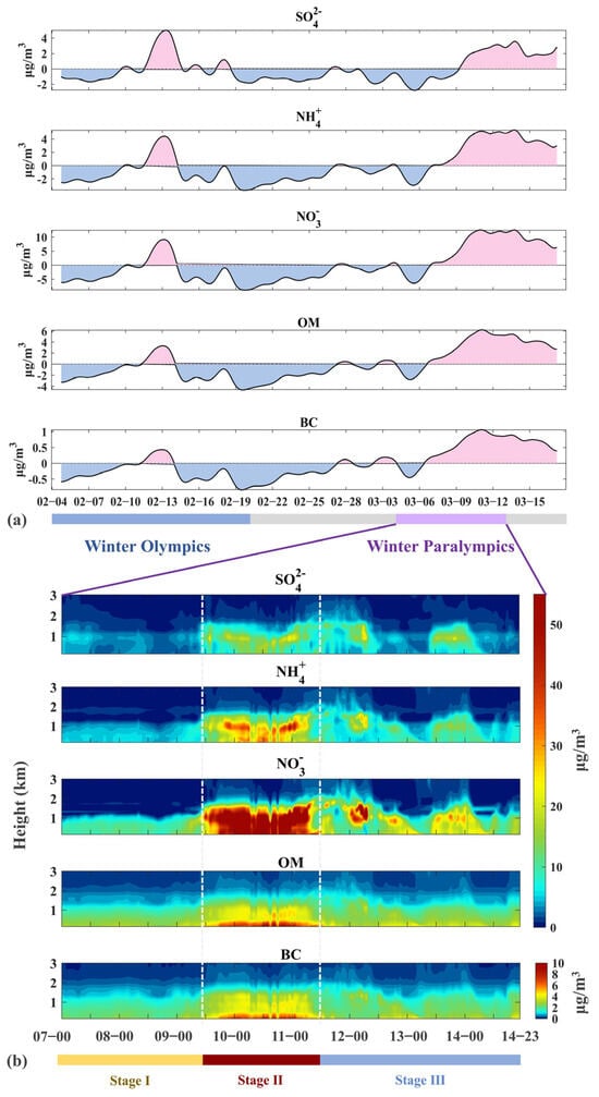
Figure 1.
(a) Meteorologically adjusted long-term components from 4 February to 17 March. (b) Vertical concentration evolution of five chemical components in the pollution process of the Winter Paralympics (from 7 March 0:00 to 14 March 23:00). Time is presented as month–day in (a) and day–hour in (b).

Table 1.
Contributions of meteorological conditions and anthropogenic emissions to the long-term components from 4 February to 17 March, and average concentrations and mean heights of maximum concentrations during Winter Paralympics pollution.
To reveal the vertical patterns and different responses of components to strict control policies and meteorology, we further conducted in-depth research into the Paralympics pollution. Figure 1b presents the vertical concentration distribution of each component from 7 March to 14 March. The transition of pollution from initiation to dispersion is clearly observed, consistent with the evolution of AOD [64] and the traditional pollution patterns observed in Beijing [19,21,28] in previous studies, including processes like lifting, transport and sinking, northwesterly wind-driven clearing, and dissipation.
Among the aerosol components, NO3− and OM were dominant, which constituted up to 37.53% and 29.37% of the total aerosol concentration, respectively (Table 1), highlighting traffic and residential sources [65,66]. The average heights of maximum concentrations for inorganic components, SO42−, NH4+, and NO3−, were all found above 600 m, with maximum heights of around 1000 m, and concentrations reaching 28.39 μg m−3, 54.00 μg m−3, and 144.07 μg m−3, respectively. The average concentration of inorganic components above 1000 m (45.92 μg m−3) exceeded that at ground level (38.70 μg m−3) by 1.19 times across the entire pollution episode, showcasing the high-altitude transport feature. Previous studies found that the contribution of SO42− increased in the free troposphere, and NO3− and NH4+ were more enriched near the surface and more uniformly distributed in the boundary layer during winter and spring in Beijing [28,67]. Our result was basically consistent with the patterns in previous studies, but showed a more profound high-altitude concentrated feature for NH4+ and NO3−, probably due to the strict local emission control. In contrast, the peak concentrations of organic components (OM and BC) were near 200 m, with maximums of 57.49 μg m−3 and 8.49 μg m−3, respectively. The average ground-level concentration (27.67 μg m−3) was 1.78 times that of the high-altitude concentration (15.52 μg m−3), indicating robust surface sources.
The pollution event during the Winter Paralympics can be divided into three stages according to the vertical evolution and meteorology impact: Stage I (0:00 7 March to 11:00 9 March), Stage II (12:00 9 March to 11:00 11 March), and Stage III (12:00 11 March to 23:00 14 March). In the following sections, we will present a comprehensive analysis of the distribution of different components, the characteristics of meteorological elements, and their impacts on the pollution evolution at each stage.
3.2. Stage I—Inorganics Originated from High-Altitude Transport and Uplifting; Organics Concentrated near Surface
Stage I showed the initiation of the pollution process, with the distinct distribution of different components. As shown in Table 2, OM was the pollutant with the highest concentration at Stage I, accounting for 41.16% of PM2.5. Inorganic components (SO42−, NH4+, and NO3−) demonstrated high concentrations at the upper level (700–800 m), while organic components (OM and BC) displayed surface-concentrated features (around 150 m). Due to the similar distribution of NO3− and NH4+ in inorganic matter [68] and OM and BC in organic matter, SO42−, NO3−, and OM were selected as examples to further analyze the vertical evolution of each component.
Table 2.
Average concentrations and mean heights of maximum pollutant concentrations during three stages.
During Stage I, SO42− demonstrated a notably higher concentration peak at 800–1000 m, achieving 4.05 μg m−3 at 919 m, and decreased to a 19% lower concentration near the surface (Figure S5), implying the contribution of high-altitude transport (Figure S7). SO42− at high altitudes consisted during the whole stage, mainly dominated by a westerly wind, first by a fast north-westerly wind, and then by a south-westerly wind with lower wind speed (Figure 2c,d). At the end of Stage I (12:00 9 March), the SO42− concentration near 1000 m surged to 13.47 μg m−3, almost 3.46 times that of the previous average concentration (3.89 μg m−3). The ratio of the high layer to low layer which increased to 2.61 indicated the transport from Hebei by a southwesterly wind at high levels (Figure 2b), in line with the SO42−-rich characteristics in the surrounding cities near Beijing [69]. The backward trajectory analysis at 150 m, 500 m, and 1000 m in Figure S4 also confirmed this result.
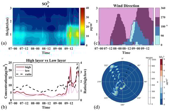
Figure 2.
Variation of SO42− and related meteorological factors during Stage I. (a) Vertical distribution of concentrations, (b) average concentrations at high layer (900–1000 m), low layer (below 200 m), and ratio of high layer to low layer, (c) wind direction, (d) concentrations and the peak concentration heights with wind speed and wind direction. Time is presented as day–hour.
NO3− showed a uniform distribution below 700 m, with concentrations of around 10 μg m−3, and decreased sharply from 700 m to 1200 m (Figure S5). Similar to SO42−, NO3− mainly had sources from three directions. However, the two westerly sources corresponded to a lower level (400–600 m) transport compared to SO42−. Meanwhile, with RH rising at 22:00 on 8 March, the ground-level NO3− increased from 9 μg m−3 to 13 μg m−3, which may be caused by the boundary layer height depletion and nighttime traffic sources [19,70]. And then the ground-level NO3− was gradually uplifted to 760 m by the vertical updraft (Figure 3b,d), probably because of the increased boundary layer height in the morning. At 10:00 on 9 March, the southwesterly transport near 1000 m combined with the uplifted sources motivated the start of the formal pollution event, and the NO3− concentration at high altitudes rose to 23.33 μg m−3 (3.23 times that of the previous average), making NO3− the earliest rising component, meanwhile the surface NO3− also showed a smaller increase (Figure 3d). During the initiation of NO3−, NO3− and RH exhibited a positive correlation, with a steeper slope and larger NO3−/BC value at a higher altitude (Figure 3e and Figure S7(b3)). This may possibly be caused by the increased contribution of secondary production from the non-homogeneous reaction of N2O5 with H2O in upper layers [71,72,73] and the upward and southern transport of NO3− and its precursors (Figures S6 and S7(a3,b3)).
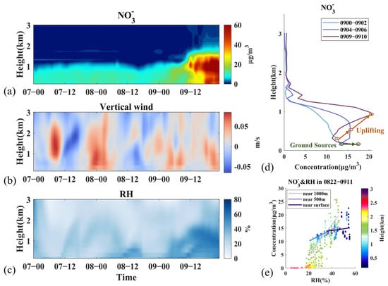
Figure 3.
Variation of NO3− and related meteorological factors during Stage I. (a) Vertical distribution of concentrations, (b) vertical wind, (c) relative humidity, (d) vertical profiles of concentrations in selected hours, (e) concentration distribution with RH from 22:00 8 March to 11:00 9 March and fitted lines at three altitudes. Time is presented as day–hour.
For organic components, OM exhibited a declining trend with increasing altitude, with maximums always observed near 150 m, signifying strong ground sources (Figure S5). OM concentrations below 300 m were above 15 μg m−3, while the concentration near 1000 m (9.17 μg m−3) was only 60% of the lower layer concentration. Similar to NO3−, nighttime traffic emission and secondary formation with increasing RH also contributed to the rise of OM concentrations at the surface level (Figure 4a,b and Figure S7(b4)). On the morning of 9 March, the vertical updraft brought part of OM to a higher level, with OM near the surface (500 m) decreasing (slightly increasing) with the vertical wind (Figure 4d). And the pollution started at 11:00 for OM, with an increasing concentration below 300 m and surface concentration reaching 27.64 μg m−3 in Beijing (Figure 4a,c). Compared with prior time, the surface concentrations of the southeast stations showed a declining trend while Beijing displayed an opposite trend, indicating the southeast transport the near surface (Figure 4c and Figure S4a).
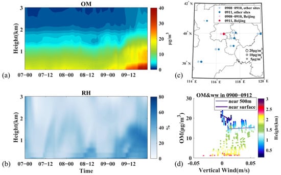
Figure 4.
Variation of OM and related meteorological factors during Stage I. (a) Vertical distribution of concentrations, (b) relative humidity, (c) in situ observed surface concentration averages at 8:00–10:00 9 March (left) and 11:00 9 March (right), red dots represent values at Beijing site, blue dots represent values at other sites, (d) concentration distribution with vertical wind from 0:00 9 March to 12:00 9 March, and fitted lines at two altitudes. Time is presented as day–hour.
In general, Stage I was characterized by a westerly high-altitude transport peak of SO42−, uniform NO3− distribution under the combined efforts of surface uplifting, high-altitude transport and secondary generation, and surface high-concentrated OM. At the end of Stage I, pollution formally started first by NO3−, followed by OM near the surface and SO42− near 1000 m. The generation of pollutants showed the contribution of regional sources to inorganic components in Beijing, which emphasized the importance of joint prevention and control at a regional scale.
3.3. Stage II—Transported Inorganics Held, Sank and Uplifted; Organics Massed Below 500 m
In Stage II, the concentrations of all components increased, reaching 2.01–5.81 times the average of Stage I (Table 2). Among them, NO3− showed the most obvious growth and became the dominant pollutant, accounting for 44.25% of PM2.5.
Compared to Stage I, SO42− displayed a similar high-altitude transport pattern, but showed another peak at 1516 m except for the 919 m peak, with 1.2–1.4 times higher concentrations than the surface level (Figure S8). The SO42− transport near 1000 m in the previous stage continued and was enhanced by the high-speed southwesterly wind (Figure S4 and ① in Figure 5), during which the static weather condition near the surface (intensive temperature inversion, increasing RH and vertical updraft) held SO42− at a high level (Figure S9). Then, SO42− showed an obvious trend of sinking, starting from 22:00 9 March and lasting until 15:00 10 March when the peak height dropped to 150 m. The high-altitude concentrations of SO42− progressively decreased from 20 μg m−3 to 8 μg m−3, while the ground-level concentrations increased by 133% (from 6 μg m−3 to 14 μg m−3), with the ratio of high-altitude to surface concentration declining sharply from 3.22 to 0.56 (Figure 5c). It was probably due to the fact that the horizontal wind minimized, the downward draft dominated below 1000 m, and the increasing RH facilitated the gravitational deposition and aqueous formation [67].

Figure 5.
Variation of SO42− and related meteorological factors during Stage II. (a) Vertical distribution of concentrations, (b) wind direction, (c) average concentrations at L0 (below 200 m), L1 (900–1000 m), L2 (1400–1600 m), and ratios of higher layers to low layer, (d) vertical profiles of concentrations in selected hours, (e) concentrations and the peak concentration heights with wind speed and wind direction. Time is presented as day–hour.
After 18:00 10 March, a resurging of SO42− concentration was driven by a shift to easterly wind (Figure S9 and ② in Figure 5), bringing the peak height back to 919 m. Later, easterly transport near 1000 m increased the SO42− concentration to 19.59 μg m−3, which may trace back to the sources from Tianjin (Figure S4c and Figure 5e). An easterly updraft further uplifted the high-concentrated SO42− to over 1500 m (Figure 5c), with the mean concentration of 1000–1600 m increasing from 7.91 to 10.36 μg m−3. The whole process of holding–sinking–lifting can also be confirmed by the vertical profiles in Figure 5d.
NO3− vertical profile was distinct from Stage I. The concentration peaked at 919 m (68.15 μg m−3) and 300 m (51.55 μg m−3) (Figure S8), with a mean peak height that rose from 413.3 m to 774.3 m (Table 2). The holding, sinking, and uplifting process of high-altitude NO3− was similar to SO42−, influenced by the vertical wind variation (Figure 6b). The high-altitude transport enhanced during the holding (Figure 6d and Figure S10(a3)), with a concentration near 1000 m that increased by 83% (45.13 to 82.59 μg m−3). During sinking, the NO3− concentration near the surface (58.54 μg m−3) rose to 2 times that of the earlier average (29.24 μg m−3). The uplifting promoted by the easterly wind uplifted the high-concentrated NO3− to a higher altitude than SO42−, reaching near 2000 m (Figure 6d).
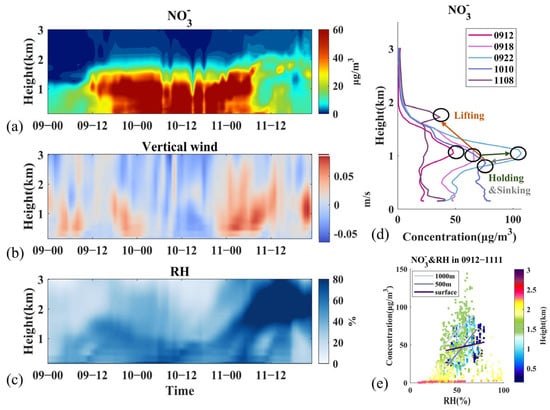
Figure 6.
Variation of NO3− and related meteorological factors during Stage II. (a) Vertical distribution of concentrations, (b) vertical wind, (c) relative humidity, (d) vertical profiles of concentrations in selected hours, (e) concentration distribution with RH from 12:00 9 March to 11:00 11 March and fitted lines at three altitudes. Time is presented as day–hour.
Similar to Stage I, despite the depicted progress, NO3− showed a stronger surface source and secondary production-influenced pattern, resulting in the peak near 300 m. The surface source started on 10 March in the morning, which may be attributed to the nighttime emission. And the secondary production extended from the surface to 1000 m (Figure S10(b3)), similar to the pattern of RH (Figure 6c). NO3− near 1000 m and 500 m increased significantly with RH, while NO3− near the surface appeared a smaller magnitude (Figure 6e). This could be explained by an intensified gas-to-particle transformation and enhanced aqueous formation of nitrate, owing to larger humidity at high altitudes [26,72,74,75].
OM retained a similar vertical profile as Stage I, but demonstrated a more pronounced gradient below 500 m. As shown in Figure 7, the OM concentration increased first near the surface, then at higher levels after 5 h, caused by southwesterly transport and upward drafts (Figure 7c). Then, all concentrations simultaneously rose, and the pattern of a high-to-low ratio was similar to the inorganics, first declining then increasing (Figure 7b). But the ratio always remained below 0.7, and the average concentration between 500 and 1200 m was only 67.45% of that below 500 m, underscoring the predominant influence of surface sources, which was probably contributed by residential sources. Secondary production made great contribution to OM under the static condition and warm and humid easterly wind (Figure S10(b4)), especially at a higher level (Figure 7d). Previous studies have suggested that high temperature and humidity, low wind speed, and significant inversion during the Paralympics were unfavorable for pollution dispersion and led to secondary production [65,76,77], which is in line with our analysis.
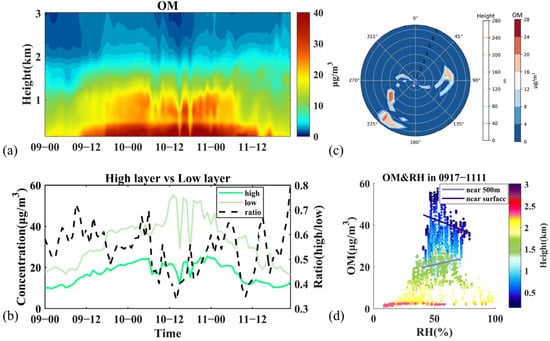
Figure 7.
Variation of OM and related meteorological factors during Stage II. (a) Vertical distribution of concentrations, (b) average concentrations at high layer (900–1000 m), low layer (below 200 m), and ratio of high layer to low layer, (c) concentrations and the peak concentration heights with wind speed and wind direction. (d) Concentration distribution with RH from 17:00 9 March to 11:00 11 March and fitted lines at two altitudes. Time is presented as day–hour.
Overall, apart from the same characteristics as Stage I, SO42− and NO3− appeared a process of holding–sinking–lifting in Stage II, and NO3− and OM showed a more pronounced secondary formation, in response to meteorological changes. As pollutants accumulated and evolved, this pattern of inorganics confirmed a high sensitivity to meteorology, showcasing the exacerbated influence of secondary formation and transport due to the lack of local emission during the strict control period.
3.4. Stage III—Transported Inorganics Sank; High-Altitude Organics Increased; High-Altitude Dispersion Started First
In Stage III, components started to disperse, with concentrations decreasing by 42–68%. OM and NO3− were the dominant pollutants, totally accounting for 65.45% of PM2.5. The peak heights of SO42−, OM, and BC increased, while those of NH4+ and NO3− decreased (Table 2).
The vertical profile of SO42− remained akin to Stage II, with peak concentrations at 919 m and 1516 m, 1.06–1.83 times higher than the surface concentration (Figure S11). Similar to Stage II, the uplifted SO42− near 1600 m began to sink downwards from 13:00 11 March. Then, in the morning of 12 March, concentrations in the range of 800–1500 m (15.91 μg m−3) first experienced a sudden increase, reaching 1.78 times that of the previous average (8.94 μg m−3), probably influenced by south-westerly transport (Figure 8d) and secondary formation at a high altitude induced by high temperature and humidity (Figure S13(b1) and Figure 8c). The ratio of 1500 m and 1000 m to the surface rose to around 4. Then, 49% of the high concentration of SO42− rapidly sank to the ground due to the boundary layer height increasing in the morning, which brought the peak height down to around 300 m and the ratio down to below 1 (Figure 8b). SO42− did not fully sink in the limited time, and the shift to the north wind eliminated concentrations at all heights. A similar but weaker progress happened at 12:00 on 13 March, but mainly concentrated near 1000 m (Figure 8e). SO42− was finally cleared in a short time by the shift to the north-westerly wind at a rate of 25 m s−1, with high altitudes 5 h earlier than the surface (Figure 8b), corresponding to the wind spear (Figure S12).
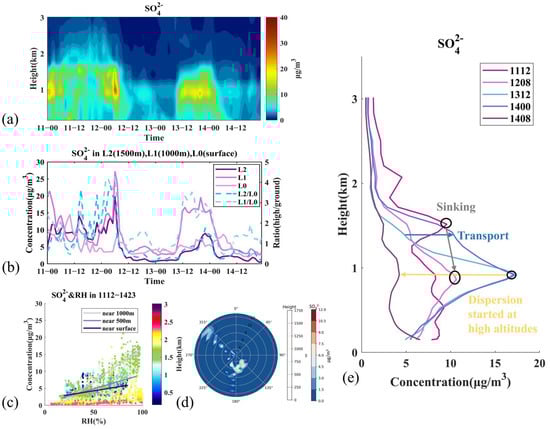
Figure 8.
Variation of SO42− and related meteorological factors during Stage III. (a) Vertical distribution of concentrations, (b) average concentrations at L0 (below 200 m), L1 (900–1000 m), L2 (1400–1600 m), and ratios of higher layers to low layers, (c) concentration distribution with RH from 12:00 11 March to 23:00 14 March, and fitted lines at three altitudes, (d) concentrations and the peak concentration heights with wind speed and wind direction, (e) vertical profiles of concentrations in selected hours. Time is presented as day–hour.
NO3− also showed a similar profile with Stage II, but with another peak near 1500 m, indicating rising concentrations at high levels (Figure S11). The uplifting altitude of NO3− was higher (near 2000 m) than the previous stage compared to SO42− (Figure 9c), but concentrations at peak heights reduced to 65.44% of the uplifting period. The south-westerly transport on 12 March in the morning enhanced the concentrations at higher levels, with the ratio soaring to over 10 (Figure 9b). The later sinking increased the concentrations at 760–1516 m to more than 30 μg m−3, with 93.65% transmitted downwards, accompanied by secondary production (Figure S13(b3) and Figure 9d), which brought the ratio down to around 2 (Figure 9b). The sinking lasted longer until 6:00 on 13 March, during which the surface NO3− concentration increased by 60%, from 13.97 μg m−3 to 22.36 μg m−3. The following new southeasterly transport-sinking process near 1000 m was aligned with SO42−, but with a more rapid increase in lower layers (Figure 9c). Moreover, after the clearance of all heights by the northwesterly wind, NO3− increased again from the surface to 700–800 m, indicating noticeable surface emission uplifting and secondary production influence (Figure S13(a3,b3)).
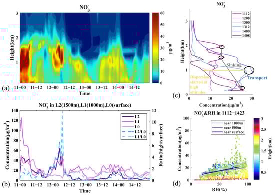
Figure 9.
Variation of NO3− and related meteorological factors during Stage III. (a) Vertical distribution of concentrations, (b) average concentrations at L0 (below 200 m), L1 (900–1000 m), L2 (1400–1600 m), and ratios of higher layers to low layer, (c) vertical profiles of concentrations in selected hours, (d) concentration distribution with RH from 12:00 11 March to 23:00 14 March, and fitted lines at three altitudes. Time is presented as day–hour.
For organic components, the profile of OM in Stage III showed a smaller slope than Stage II, suggesting the weakening of surface sources (Figure S11). Meanwhile, the influence of southern high-altitude transport strengthened, indicated by the peak concentrations of 12.31–13.64 μg m−3 near 1200 m during 5:00–7:00 on 12 March and the increasing ratio of up to 1.05 (Figure S13(a4) and Figure 10). The surface concentration increased from 12:00 on 12 March to 7:00 on 13 March (Figure 10c), driven by the synergy of sinking, emissions, probable southeastern transport from Tianjin, and accompanied secondary production (Figure 10c,d and Figure S13(b4)), especially in the early morning of 13 March when the surface concentration rose to more than 25 μg m−3 and the ratio fell back to 0.34 (Figure 10b). The final clearance process was similar to other components.
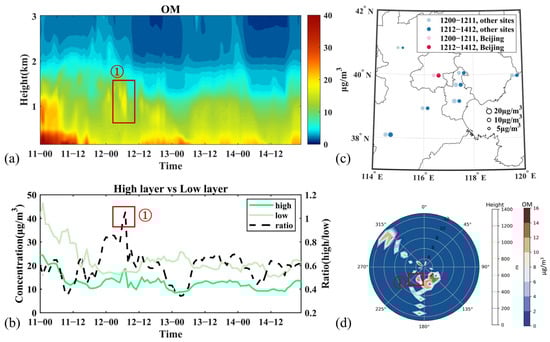
Figure 10.
Variation of OM and related meteorological factors during Stage III. (a) Vertical distribution of concentrations, (b) average concentrations at high layer (900–1000 m), low layer (below 200 m), and ratio of high layer to low layer, (c) in situ observed surface concentration averages at 0:00–11:00 on 12 March (left) and 12:00 on 12 March–12:00 on 14 March (right), red dots represent values at Beijing site, blue dots represent values at other sites, (d) concentrations and the peak concentration heights with wind speed and wind direction. Time is presented as day–hour.
In summary, Stage III demonstrated stronger characteristics of SO42− and OM high-altitude transport and NO3− sinking. All components showed a clearance first from higher layers then to lower layers, driven by the corresponding wind shift to the northwest.
4. Discussion
In this study, we used a unique vertical–temporal continuous vertical mass concentration dataset of key PM2.5 chemical components (SO42−, NH4+, NO3−, OM, and BC), retrieved from sun–sky photometer and lidar observation data, to analyze the vertical patterns of different components and their response to pollution control and meteorology in March 2022 Beijing. First through KZ filtering, it was found that emission contributed to 51.12% of PM2.5 during the Winter Paralympics, while meteorology played a more important role for inorganic components (SO42− and NO3−). It was similar with previous studies, but showing a larger meteorological contribution. Components displayed distinct patterns in three stages during the event. Overall, inorganics and organics showed characteristics of high-altitude transport and surface source, respectively, with NO3− and OM dominating.
Among inorganic components, SO42− showed a high-altitude transport peak at 919 m. The injected SO42− at 1000 m by southwesterly wind first experienced a holding period, due to the static weather condition; then began to sink, with the average high-altitude (surface) concentration progressively decreasing (increasing) from 20 (6) to 8 (14) μg m−3. Later, SO42− resurged to a higher altitude of 1600 m by an easterly updraft. During Stage III, uplifted SO42− transported downwards and another transport near 1000 m occurred, with 49% SO42− sunk to ground. Despite the characteristics of high-altitude transport for inorganics, NH4+ and NO3− also showed features of secondary production and ground source contribution, demonstrated by the relatively uniform distribution below 700 m in Stage I, a higher lifting altitude than SO42− in Stage II, and the sinking proportion of 93.65% in Stage III.
By contrast, organic components (OM and BC) exhibited declining concentrations with increasing altitudes, signifying dominant ground sources. The average concentration near the surface was 1.79 times of that near 1000 m. Across three stages, the influence of high-altitude transport appeared larger with time. As pollution triggered near the surface, high-altitude (500–1200 m) concentrations also increased, but only accounted for 67.45% of the concentration below 500 m. But in Stage III, the peak heights reached above 1000 m for the first time and lasted 3 h, under the impact of high-altitude transport and sinking. Moreover, OM also showed a strong secondary production feature compared to BC, thus influenced more by meteorological factors.
Through analyzing the vertical evolution of different components by using Winter Paralympics pollution as an example, we provide a comprehensive depiction of component vertical patterns in response to meteorology under strict emission control. The observed patterns of chemical components during the Winter Paralympics case underscored the synergy of local emission, transport, and secondary formation, with distinct sensitivity of different components to these elements. Local emission control magnified the impact of transport and formation, as specifically demonstrated by the patterns of inorganic compounds. The presence of a southwest inorganic source at higher altitudes and an eastern organic source near the surface aligns with the characteristics of large coal combustion and heavy industrial emissions in Hebei and Tianjin, respectively [69,78].
According to these patterns, the contribution of regional sources to inorganic components in Beijing underlined that joint prevention and control of the emission of precursors (SO2, NO2) at a regional scale should be strengthened. For organics and NO3−, more attention should be paid to the local emission of NOx and VOCs from residential and transportation sources in Beijing. Moreover, our study demonstrated the exacerbated impact of meteorological conditions during a strict control period, suggesting that stricter regional control methods need to be adopted in advance when unfavorable meteorological conditions are forecasted. These findings contribute to a deeper understanding of aerosol characteristics in Beijing and helpful data assistance for component-targeted emission control strategies.
Despite the insights provided by this study, limitations such as a short study duration and restricted spatial coverage will be addressed in the future research to portray a more comprehensive view of the three-dimensional evolution of PM2.5 components and to further elucidate the complex interactions between emissions, meteorology, and pollutant transport.
Supplementary Materials
The following supporting information can be downloaded at: https://www.mdpi.com/article/10.3390/rs17071151/s1, Figure S1: Data used in this study. (a) Location of observation data, (b) Dual-wavelength polarization Mie lidar, (c) Example profile of lidar signals on 0:00 9 March, (d) Example profile of optical data on 0:00 9 March, (e) Example profile of chemical data on 0:00 9 March; Figure S2: Comparison of retrieved mass concentration and observation data. Dates are presented as month–day; Figure S3: (a) Vertical profile of aircraft measurement in 2016 winter; (b) Vertical profile and evaluation indices of retrieved results; Figure S4: Backward trajectory analysis result of (a) Stage I, (b, c) Stage II, (d) Stage III; Figure S5: Vertical profiles of average pollutant concentrations in Stage I; Figure S6: Temporal and spatial variations of meteorological factors in Stage I. (a) Horizontal wind speed, (b) wind direction, (c) vertical velocity, (d) temperature, (e) temperature gradient, (f) relative humidity. Dates are presented as day–hour; Figure S7: (a1–a5) Changes in the ratio of pollutant concentrations at each layer to the ground level in Stage I, (b1–b4) Changes in the ratio of SO42−, NH4+, NO3−, and OM to BC in Stage I; Figure S8: Vertical profiles of average pollutant concentrations in Stage II; Figure S9: Temporal and spatial variations of meteorological factors in Stage II. (a) horizontal wind speed, (b) wind direction, (c) vertical velocity, (d) temperature, (e) temperature gradient, (f) relative humidity. Dates are presented as day–hour; Figure S10: (a1–a5) Changes in the ratio of pollutant concentrations at each layer to the ground level in Stage II, (b1–b4) Changes in the ratio of SO42−, NH4+, NO3−, and OM to BC in Stage II; Figure S11: Vertical profiles of average pollutant concentrations in Stage III; Figure S12: Temporal and spatial variations of meteorological factors in Stage III. (a) Horizontal wind speed, (b) wind direction, (c) vertical velocity, (d) temperature, (e) temperature gradient, (f) relative humidity. Dates are presented as day–hour; Figure S13: (a1–a5) Changes in the ratio of pollutant concentrations at each layer to the ground level in Stage III, (b1–b4) Changes in the ratio of SO42−, NH4+, NO3−, and OM to BC in Stage III; Table S1: Information of in situ chemical observation sites; Table S2: Variance contribution of each component from 14 February to 17 March and average meteorological elements during the Winter Olympics and Paralympics.
Author Contributions
Conceptualization, T.Y. and Y.S. (Yifan Song); methodology, T.Y.; software, H.L.; validation, Y.T. (Yutong Tian) and Y.T. (Yining Tan); formal analysis, Y.S. (Yifan Song); investigation, Y.S. (Yifan Song); resources, P.T.; data curation, H.L.; writing—original draft preparation, Y.S. (Yifan Song); writing—review and editing, Y.S. (Yifan Song) and T.Y.; visualization, Y.S. (Yifan Song); supervision, Y.S. (Yele Sun) and Z.W. All authors have read and agreed to the published version of the manuscript.
Funding
This work was supported in part by the National Key Research and Development Program for Young Scientists of China (No. 2022YFC3704000), and in part by the National Natural Science Foundation of China (No. 42275122).
Data Availability Statement
The raw data supporting the conclusions of this article will be made available by the authors on request.
Acknowledgments
We are thankful for the technical support of the National large Scientific and Technological Infrastructure “Earth System Numerical Simulation Facility” (https://cstr.cn/31134.02.EL, accessed on 23 March 2025). Ting Yang would like to express gratitude towards the Program of the Youth Innovation Promotion Association (CAS).
Conflicts of Interest
The authors declare no conflicts of interest.
References
- Li, J.; Carlson, B.E.; Yung, Y.L.; Lv, D.; Hansen, J.; Penner, J.E.; Liao, H.; Ramaswamy, V.; Kahn, R.A.; Zhang, P.; et al. Scattering and absorbing aerosols in the climate system. Nat. Rev. Earth Environ. 2022, 3, 363–379. [Google Scholar]
- Weare, B.C.; Temkin, R.L.; Snell, F.M. Aerosol and Climate: Some Further Considerations. Science 1974, 186, 827–828. [Google Scholar] [PubMed]
- Zhai, J.; Shao, S.; Yang, X.; Zeng, Y.; Fu, T.-M.; Zhu, L.; Shen, H.; Ye, J.; Wang, C.; Tao, S. Chemically Resolved Respiratory Deposition of Ultrafine Particles Characterized by Number Concentration in the Urban Atmosphere. Environ. Sci. Technol. 2024, 58, 16507–16516. [Google Scholar]
- Li, Q.; Zhang, H.; Cai, X.; Song, Y.; Zhu, T. The impacts of the atmospheric boundary layer on regional haze in North China. npj Clim. Atmos. Sci. 2021, 4, 9. [Google Scholar]
- Shi, Y.; Liu, L.; Hu, F.; Fan, G.; Huo, J. Nocturnal Boundary Layer Evolution and Its Impacts on the Vertical Distributions of Pollutant Particulate Matter. Atmosphere 2021, 12, 610. [Google Scholar] [CrossRef]
- Sun, T.; Wu, C.; Wu, D.; Liu, B.; Sun, J.Y.; Mao, X.; Yang, H.; Deng, T.; Song, L.; Li, M.; et al. Time-resolved black carbon aerosol vertical distribution measurements using a 356-m meteorological tower in Shenzhen. Theor. Appl. Climatol. 2020, 140, 1263–1276. [Google Scholar]
- Zheng, C.; Zhao, C.; Zhu, Y.; Wang, Y.; Shi, X.; Wu, X.; Chen, T.; Wu, F.; Qiu, Y. Analysis of influential factors for the relationship between PM2.5 and AOD in Beijing. Atmos. Chem. Phys. 2017, 17, 13473–13489. [Google Scholar]
- Zhou, S.; Wu, L.; Guo, J.; Chen, W.; Wang, X.; Zhao, J.; Cheng, Y.; Huang, Z.; Zhang, J.; Sun, Y.; et al. Measurement report: Vertical distribution of atmospheric particulate matter within the urban boundary layer in southern China—Size-segregated chemical composition and secondary formation through cloud processing and heterogeneous reactions. Atmos. Chem. Phys. 2020, 20, 6435–6453. [Google Scholar]
- Shao, P.; Tian, H.; Sun, Y.; Liu, H.; Wu, B.; Liu, S.; Liu, X.; Wu, Y.; Liang, W.; Wang, Y.; et al. Characterizing remarkable changes of severe haze events and chemical compositions in multi-size airborne particles (PM1, PM2.5 and PM10) from January 2013 to 2016–2017 winter in Beijing, China. Atmos. Environ. 2018, 189, 133–144. [Google Scholar]
- Zhai, S.; Jacob, D.J.; Wang, X.; Shen, L.; Li, K.; Zhang, Y.; Gui, K.; Zhao, T.; Liao, H. Fine particulate matter (PM2.5) trends in China, 2013–2018: Separating contributions from anthropogenic emissions and meteorology. Atmos. Chem. Phys. 2019, 19, 11031–11041. [Google Scholar]
- Zhao, L.; Wang, L.; Tan, J.; Duan, J.; Ma, X.; Zhang, C.; Ji, S.; Qi, M.; Lu, X.; Wang, Y.; et al. Changes of chemical composition and source apportionment of PM2.5 during 2013–2017 in urban Handan, China. Atmos. Environ. 2019, 206, 119–131. [Google Scholar]
- Zheng, B.; Tong, D.; Li, M.; Liu, F.; Hong, C.; Geng, G.; Li, H.; Li, X.; Peng, L.; Qi, J.; et al. Trends in China’s anthropogenic emissions since 2010 as the consequence of clean air actions. Atmos. Chem. Phys. 2018, 18, 14095–14111. [Google Scholar]
- Wang, Y.; Gao, W.; Wang, S.; Song, T.; Gong, Z.; Ji, D.; Wang, L.; Liu, Z.; Tang, G.; Huo, Y.; et al. Contrasting trends of PM2.5 and surface-ozone concentrations in China from 2013 to 2017. Natl. Sci. Rev. 2020, 7, 1331–1339. [Google Scholar]
- Wang, Y.; Li, W.; Gao, W.; Liu, Z.; Tian, S.; Shen, R.; Ji, D.; Wang, S.; Wang, L.; Tang, G.; et al. Trends in particulate matter and its chemical compositions in China from 2013–2017. Sci. China-Earth Sci. 2019, 62, 1857–1871. [Google Scholar]
- Geng, G.; Liu, Y.; Liu, Y.; Liu, S.; Cheng, J.; Yan, L.; Wu, N.; Hu, H.; Tong, D.; Zheng, B.; et al. Efficacy of China’s clean air actions to tackle PM2.5 pollution between 2013 and 2020. Nat. Geosci. 2024, 17, 987–994. [Google Scholar]
- Xu, Q.; Wang, S.; Jiang, J.; Bhattarai, N.; Li, X.; Chang, X.; Qiu, X.; Zheng, M.; Hua, Y.; Hao, J. Nitrate dominates the chemical composition of PM2.5 during haze event in Beijing, China. Sci. Total Environ. 2019, 689, 1293–1303. [Google Scholar]
- Li, H.; Cheng, J.; Zhang, Q.; Zheng, B.; Zhang, Y.; Zheng, G.; He, K. Rapid transition in winter aerosol composition in Beijing from 2014 to 2017: Response to clean air actions. Atmos. Chem. Phys. 2019, 19, 11485–11499. [Google Scholar]
- Guo, Y. Characteristics of size-segregated carbonaceous aerosols in the Beijing-Tianjin-Hebei region. Environ. Sci. Pollut. Res. 2016, 23, 13918–13930. [Google Scholar]
- Lei, L.; Sun, Y.; Ouyang, B.; Qiu, Y.; Xie, C.; Tang, G.; Zhou, W.; He, Y.; Wang, Q.; Cheng, X.; et al. Vertical Distributions of Primary and Secondary Aerosols in Urban Boundary Layer: Insights into Sources, Chemistry, and Interaction with Meteorology. Environ. Sci. Technol. 2021, 55, 4542–4552. [Google Scholar]
- Öztürk, F.; Bahreini, R.; Wagner, N.L.; Dubé, W.P.; Young, C.J.; Brown, S.S.; Brock, C.A.; Ulbrich, I.M.; Jimenez, J.L.; Cooper, O.R.; et al. Vertically resolved chemical characteristics and sources of submicron aerosols measured on a Tall Tower in a suburban area near Denver, Colorado in winter. J. Geophys. Res.-Atmos. 2013, 118, 13591–13605. [Google Scholar]
- Du, W.; Zhao, J.; Wang, Y.; Zhang, Y.; Wang, Q.; Xu, W.; Chen, C.; Han, T.; Zhang, F.; Li, Z.; et al. Simultaneous measurements of particle number size distributions at ground level and 260 m on a meteorological tower in urban Beijing, China. Atmos. Chem. Phys. 2017, 17, 6797–6811. [Google Scholar]
- Wu, H.; Zhang, Y.-f.; Han, S.-q.; Wu, J.-h.; Bi, X.-h.; Shi, G.-l.; Wang, J.; Yao, Q.; Cai, Z.-y.; Liu, J.-l.; et al. Vertical characteristics of PM2.5 during the heating season in Tianjin, China. Sci. Total Environ. 2015, 523, 152–160. [Google Scholar] [PubMed]
- Chen, Y.-C.; Chang, C.-C.; Chen, W.-N.; Tsai, Y.-J.; Chang, S.-Y. Determination of the vertical profile of aerosol chemical species in the microscale urban environment. Environ. Pollut. 2018, 243, 1360–1367. [Google Scholar]
- Wu, H.; Taylor, J.W.; Szpek, K.; Langridge, J.M.; Williams, P.I.; Flynn, M.; Allan, J.D.; Abel, S.J.; Pitt, J.; Cotterell, M.I.; et al. Vertical variability of the properties of highly aged biomass burning aerosol transported over the southeast Atlantic during CLARIFY-2017. Atmos. Chem. Phys. 2020, 20, 12697–12719. [Google Scholar]
- Hatakeyama, S.; Ikeda, K.; Hanaoka, S.; Watanabe, I.; Arakaki, T.; Bandow, H.; Sadanaga, Y.; Kato, S.; Kajii, Y.; Zhang, D.; et al. Aerial observations of air masses transported from East Asia to the Western Pacific: Vertical structure of polluted air masses. Atmos. Environ. 2014, 97, 456–461. [Google Scholar]
- Brooks, J.; Allan, J.D.; Williams, P.I.; Liu, D.; Fox, C.; Haywood, J.; Langridge, J.M.; Highwood, E.J.; Kompalli, S.K.; O’Sullivan, D.; et al. Vertical and horizontal distribution of submicron aerosol chemical composition and physical characteristics across northern India during pre-monsoon and monsoon seasons. Atmos. Chem. Phys. 2019, 19, 5615–5634. [Google Scholar]
- Kim, J.-M.; Lee, H.-J.; Jo, H.-Y.; Jo, Y.-J.; Kim, C.-H. Vertical Characteristics of Secondary Aerosols Observed in the Seoul and Busan Metropolitan Areas of Korea during KORUS-AQ and Associations with Meteorological Conditions. Atmosphere 2021, 12, 1451. [Google Scholar] [CrossRef]
- Liu, Q.; Quan, J.; Jia, X.; Sun, Z.; Li, X.; Gao, Y.; Liu, Y. Vertical Profiles of Aerosol Composition over Beijing, China: Analysis of In Situ Aircraft Measurements. J. Atmos. Sci. 2019, 76, 231–245. [Google Scholar]
- Li, J.; Fu, Q.; Huo, J.; Wang, D.; Yang, W.; Bian, Q.; Duan, Y.; Zhang, Y.; Pan, J.; Lin, Y.; et al. Tethered balloon-based black carbon profiles within the lower troposphere of Shanghai in the 2013 East China smog. Atmos. Environ. 2015, 123, 327–338. [Google Scholar]
- Rosati, B.; Gysel, M.; Rubach, F.; Mentel, T.F.; Goger, B.; Poulain, L.; Schlag, P.; Miettinen, P.; Pajunoja, A.; Virtanen, A.; et al. Vertical profiling of aerosol hygroscopic properties in the planetary boundary layer during the PEGASOS campaigns. Atmos. Chem. Phys. 2016, 16, 7295–7315. [Google Scholar]
- Arola, A.; Schuster, G.; Myhre, G.; Kazadzis, S.; Dey, S.; Tripathi, S.N. Inferring absorbing organic carbon content from AERONET data. Atmos. Chem. Phys. 2011, 11, 215–225. [Google Scholar]
- Schuster, G.L.; Dubovik, O.; Holben, B.N.; Clothiaux, E.E. Inferring black carbon content and specific absorption from Aerosol Robotic Network (AERONET) aerosol retrievals. J. Geophys. Res.-Atmos. 2005, 110, D10S17. [Google Scholar]
- Xie, Y.S.; Li, Z.Q.; Zhang, Y.X.; Zhang, Y.; Li, D.H.; Li, K.T.; Xu, H.; Zhang, Y.; Wang, Y.Q.; Chen, X.F.; et al. Estimation of atmospheric aerosol composition from ground-based remote sensing measurements of Sun-sky radiometer. J. Geophys. Res.-Atmos. 2017, 122, 498–518. [Google Scholar]
- Zhang, Y.; Li, Z.; Chen, Y.; de Leeuw, G.; Zhang, C.; Xie, Y.; Li, K. Improved inversion of aerosol components in the atmospheric column from remote sensing data. Atmos. Chem. Phys. 2020, 20, 12795–12811. [Google Scholar]
- Zhang, Y.; Li, Z.; Zhang, Y.; Li, D.; Qie, L.; Che, H.; Xu, H. Estimation of aerosol complex refractive indices for both fine and coarse modes simultaneously based on AERONET remote sensing products. Atmos. Meas. Tech. 2017, 10, 3203–3213. [Google Scholar]
- Nishizawa, T.; Sugimoto, N.; Matsui, I.; Shimizu, A.; Tatarov, B.; Okamoto, H. Algorithm to Retrieve Aerosol Optical Properties From High-Spectral-Resolution Lidar and Polarization Mie-Scattering Lidar Measurements. IEEE Trans. Geosci. Remote Sens. 2008, 46, 4094–4103. [Google Scholar]
- Veselovskii, I.; Hu, Q.; Goloub, P.; Podvin, T.; Barchunov, B.; Korenskii, M. Combining Mie–Raman and fluorescence observations: A step forward in aerosol classification with lidar technology. Atmos. Meas. Tech. 2022, 15, 4881–4900. [Google Scholar]
- Li, L.; Che, H.; Derimian, Y.; Dubovik, O.; Schuster, G.L.; Chen, C.; Li, Q.; Wang, Y.; Guo, B.; Zhang, X. Retrievals of fine mode light-absorbing carbonaceous aerosols from POLDER/PARASOL observations over East and South Asia. Remote Sens. Environ. 2020, 247, 111913. [Google Scholar]
- Li, L.; Dubovik, O.; Derimian, Y.; Schuster, G.L.; Lapyonok, T.; Litvinov, P.; Ducos, F.; Fuertes, D.; Chen, C.; Li, Z.; et al. Retrieval of aerosol components directly from satellite and ground-based measurements. Atmos. Chem. Phys. 2019, 19, 13409–13443. [Google Scholar]
- Wang, F.; Yang, T.; Wang, Z.; Wang, H.; Chen, X.; Sun, Y.; Li, J.; Tang, G.; Chai, W. Algorithm for vertical distribution of boundary layer aerosol components in remote-sensing data. Atmos. Meas. Technol. 2022, 15, 6127–6144. [Google Scholar]
- Lei, F.; Dong, X.; Ma, X. Prediction of PM2.5 concentration considering temporal and spatial features: A case study of Fushun, Liaoning Province. J. Intell. Fuzzy Syst. 2020, 39, 8015–8025. [Google Scholar]
- Li, T.; Hua, M.; Wu, X. A Hybrid CNN-LSTM Model for Forecasting Particulate Matter (PM2.5). IEEE Access 2020, 8, 26933–26940. [Google Scholar] [CrossRef]
- Liu, S.; Geng, G.; Xiao, Q.; Zheng, Y.; Liu, X.; Cheng, J.; Zhang, Q. Tracking Daily Concentrations of PM2.5 Chemical Composition in China since 2000. Environ. Sci. Technol. 2022, 56, 16517–16527. [Google Scholar] [PubMed]
- Wang, T.; Du, H.; Cheng, W.; Zhao, Z.; Zhang, J.; Zhou, C. Influence of meteorological conditions on the air quality during the 2022 Winter Olympics in Beijing. Front. Environ. Sci. 2022, 10, 987272. [Google Scholar]
- Wu, Q.; Wu, Z.; Li, S.; Chen, Z. The Impact of the Beijing Winter Olympic Games on Air Quality in the Beijing–Tianjin–Hebei Region: A Quasi-Natural Experiment Study. Sustainability 2023, 15, 11252. [Google Scholar] [CrossRef]
- Yang, T.; Wang, Z.; Zhang, B.; Wang, X.; Wang, W.; Gbauidi, A.; Gong, Y. Evaluation of the effect of air pollution control during the Beijing 2008 Olympic Games using Lidar data. Chin. Sci. Bull. 2010, 55, 1311–1316. [Google Scholar]
- Liu, Q.; Liu, D.; Gao, Q.; Tian, P.; Wang, F.; Zhao, D.; Bi, K.; Wu, Y.; Ding, S.; Hu, K.; et al. Vertical characteristics of aerosol hygroscopicity and impacts on optical properties over the North China Plain during winter. Atmos. Chem. Phys. 2020, 20, 3931–3944. [Google Scholar]
- Zhang, R.; Jing, J.; Tao, J.; Hsu, S.C.; Wang, G.; Cao, J.; Lee, C.S.L.; Zhu, L.; Chen, Z.; Zhao, Y.; et al. Chemical characterization and source apportionment of PM2.5 in Beijing: Seasonal perspective. Atmos. Chem. Phys. 2013, 13, 7053–7074. [Google Scholar] [CrossRef]
- Li, H.; Yang, T.; Du, Y.; Tan, Y.; Wang, Z. Interpreting hourly mass concentrations of PM2.5 chemical components with an optimal deep-learning model. J. Environ. Sci. 2025, 151, 125–139. [Google Scholar]
- Benavent-Oltra, J.A.; Casquero-Vera, J.A.; Román, R.; Lyamani, H.; Pérez-Ramírez, D.; Granados-Muñoz, M.J.; Herrera, M.; Cazorla, A.; Titos, G.; Ortiz-Amezcua, P.; et al. Overview of the SLOPE I and II campaigns: Aerosol properties retrieved with lidar and sun–sky photometer measurements. Atmos. Chem. Phys. 2021, 21, 9269–9287. [Google Scholar]
- Benavent-Oltra, J.A.; Román, R.; Granados-Muñoz, M.J.; Pérez-Ramírez, D.; Ortiz-Amezcua, P.; Denjean, C.; Lopatin, A.; Lyamani, H.; Torres, B.; Guerrero-Rascado, J.L.; et al. Comparative assessment of GRASP algorithm for a dust event over Granada (Spain) during ChArMEx-ADRIMED 2013 campaign. Atmos. Meas. Tech. 2017, 10, 4439–4457. [Google Scholar]
- Bovchaliuk, V.; Goloub, P.; Podvin, T.; Veselovskii, I.; Tanre, D.; Chaikovsky, A.; Dubovik, O.; Mortier, A.; Lopatin, A.; Korenskiy, M.; et al. Comparison of aerosol properties retrieved using GARRLiC, LIRIC, and Raman algorithms applied to multi-wavelength lidar and sun/sky-photometer data. Atmos. Meas. Technol. 2016, 9, 3391–3405. [Google Scholar]
- Marcos, C.R.; Pedrós, R.; Gómez-Amo, J.L.; Utrillas, M.P.; Martínez-Lozano, J.A. Analysis of Desert Dust Outbreaks Over Southern Europe Using CALIOP Data and Ground-Based Measurements. IEEE Trans. Geosci. Remote Sens. 2016, 54, 744–756. [Google Scholar]
- Tsekeri, A.; Lopatin, A.; Amiridis, V.; Marinou, E.; Igloffstein, J.; Siomos, N.; Solomos, S.; Kokkalis, P.; Engelmann, R.; Baars, H.; et al. GARRLiC and LIRIC: Strengths and limitations for the characterization of dust and marine particles along with their mixtures. Atmos. Meas. Technol. 2017, 10, 4995–5016. [Google Scholar]
- Flaum, J.B.; Rao, S.T.; Zurbenko, I.G. Moderating the Influence of Meteorological Conditions on Ambient Ozone Concentrations. J. Air Waste Manage. Assoc. 1996, 46, 35–46. [Google Scholar]
- Rao, S.T.; Zurbenko, I.G. Detecting and Tracking Changes in Ozone Air Quality. J. Air Waste Manage. Assoc. 1994, 44, 1089–1092. [Google Scholar]
- Wise, E.K.; Comrie, A.C. Extending the Kolmogorov-Zurbenko filter: Application to ozone, particulate matter, and meteorological trends. J. Air Waste Manage. Assoc. 2005, 55, 1208–1216. [Google Scholar] [CrossRef]
- Yang, W.; Zurbenko, I. Kolmogorov–Zurbenko filters. Wiley Interdiscip. Rev.-Comput. Stat. 2010, 2, 340–351. [Google Scholar]
- Milanchus, M.L.; Rao, S.T.; Zurbenko, I.G. Evaluating the Effectiveness of Ozone Management Efforts in the Presence of Meteorological Variability. J. Air Waste Manage. Assoc. 1998, 48, 201–215. [Google Scholar] [CrossRef]
- Kumari, S.; Jayaraman, G.; Ghosh, C. Analysis of long-term ozone trend over Delhi and its meteorological adjustment. Int. J. Environ. Sci. Technol. 2013, 10, 1325–1336. [Google Scholar]
- Zhang, J.Q.; Wang, Y.Q.; Gao, S.; Chen, L.; Mao, J.; Sun, Y.L.; Ma, Z.X.; Xiao, J.; Zhang, H. Study on the relationship between meteorological elements and air pollution at different time scales based on KZ filtering. China Environ. Sci. 2018, 38, 3662–3672. [Google Scholar]
- Zhao, Y.; Yang, T.; Wang, Z.; He, L.; Wu, L.; Cui, Y. Effectiveness of Air Pollution Control Efforts in Beijing–Tianjin–Hebei Region during 2013–2018 Based on the Kolmogorov–Zurbenko Filter. Climatic Environ. Res. 2020, 25, 499–509. [Google Scholar]
- Liu, Y.; Xu, X.; Yang, X.; He, J.; Ji, D.; Wang, Y. Significant Reduction in Fine Particulate Matter in Beijing during 2022 Beijing Winter Olympics. Environ. Sci. Technol. Lett. 2022, 9, 822–828. [Google Scholar]
- Lu, T.; Li, Z.; Chen, Y.; Bu, Z.; Wang, X. Research on Lidar Network Observation of Aerosol and Pollution in Beijing 2022 Winter Olympics. Atmosphere 2022, 13, 1901. [Google Scholar] [CrossRef]
- Chu, F.; Gong, C.; Sun, S.; Li, L.; Yang, X.; Zhao, W. Air Pollution Characteristics during the 2022 Beijing Winter Olympics. Int. J. Environ. Res. Public Health 2022, 19, 11616. [Google Scholar]
- Hu, Q.; Liu, C.; Li, Q.; Liu, T.; Ji, X.; Zhu, Y.; Xing, C.; Liu, H.; Tan, W.; Gao, M. Vertical profiles of the transport fluxes of aerosol and its precursors between Beijing and its southwest cities. Environ. Pollut. 2022, 312, 119988. [Google Scholar]
- Wang, Q.; Du, W.; Sun, Y.; Wang, Z.; Tang, G.; Zhu, J. Submicron-scale aerosol above the city canopy in Beijing in spring based on in-situ meteorological tower measurements. Atmos. Res. 2022, 271, 106128. [Google Scholar]
- Yang, T.; Li, H.; Xu, W.; Song, Y.; Xu, L.; Wang, H.; Wang, F.; Sun, Y.; Wang, Z.; Fu, P. Strong Impacts of Regional Atmospheric Transport on the Vertical Distribution of Aerosol Ammonium over Beijing. Environ. Sci. Technol. Lett. 2024, 11, 29–34. [Google Scholar]
- Liu, P.; Zhang, C.; Xue, C.; Mu, Y.; Liu, J.; Zhang, Y.; Tian, D.; Ye, C.; Zhang, H.; Guan, J. The contribution of residential coal combustion to atmospheric PM2. 5 in northern China during winter. Atmos. Chem. Phys. 2017, 17, 11503–11520. [Google Scholar]
- Xiang, Y.; Zhang, T.; Ma, C.; Lv, L.; Liu, J.; Liu, W.; Cheng, Y. Lidar vertical observation network and data assimilation reveal key processes driving the 3-D dynamic evolution of PM2.5 concentrations over the North China Plain. Atmos. Chem. Phys. 2021, 21, 7023–7037. [Google Scholar]
- Fu, X.; Wang, T.; Gao, J.; Wang, P.; Liu, Y.; Wang, S.; Zhao, B.; Xue, L. Persistent Heavy Winter Nitrate Pollution Driven by Increased Photochemical Oxidants in Northern China. Environ. Sci. Technol. 2020, 54, 3881–3889. [Google Scholar] [PubMed]
- Wang, H.; Lu, K.; Chen, X.; Zhu, Q.; Wu, Z.; Wu, Y.; Sun, K. Fast particulate nitrate formation via N2O5 uptake aloft in winter in Beijing. Atmos. Chem. Phys. 2018, 18, 10483–10495. [Google Scholar]
- Wang, Y.; Liu, J.; Jiang, F.; Chen, Z.; Wu, L.; Zhou, S.; Pei, C.; Kuang, Y.; Cao, F.; Zhang, Y.; et al. Vertical measurements of stable nitrogen and oxygen isotope composition of fine particulate nitrate aerosol in Guangzhou city: Source apportionment and oxidation pathway. Sci. Total Environ. 2023, 865, 161239. [Google Scholar]
- Morgan, W.T.; Allan, J.D.; Bower, K.N.; Esselborn, M.; Harris, B.; Henzing, J.S.; Highwood, E.J.; Kiendler-Scharr, A.; McMeeking, G.R.; Mensah, A.A.; et al. Enhancement of the aerosol direct radiative effect by semi-volatile aerosol components: Airborne measurements in North-Western Europe. Atmos. Chem. Phys. 2010, 10, 8151–8171. [Google Scholar]
- Neuman, J.A.; Nowak, J.B.; Brock, C.A.; Trainer, M.; Fehsenfeld, F.C.; Holloway, J.S.; Hübler, G.; Hudson, P.K.; Murphy, D.M.; Nicks, D.K., Jr.; et al. Variability in ammonium nitrate formation and nitric acid depletion with altitude and location over California. J. Geophys. Res.-Atmos. 2003, 108, 4557. [Google Scholar]
- Wang, H.; Sun, Z.; Li, H.; Gao, Y.; Wu, J.; Cheng, T. Vertical-distribution Characteristics of Atmospheric Aerosols under Different Thermodynamic Conditions in Beijing. Aerosol Air Qual. Res. 2018, 18, 2775–2787. [Google Scholar]
- Wang, Y.; Shi, M.; Lv, Z.; Liu, H.; He, K. Local and regional contributions to PM2.5 in the Beijing 2022 Winter Olympics infrastructure areas during haze episodes. Front. Env. Sci. Eng. 2021, 15, 140. [Google Scholar]
- Zhao, P.S.; Dong, F.; He, D.; Zhao, X.J.; Zhang, X.L.; Zhang, W.Z.; Yao, Q.; Liu, H.Y. Characteristics of concentrations and chemical compositions for PM2.5 in the region of Beijing, Tianjin, and Hebei, China. Atmos. Chem. Phys. 2013, 13, 4631–4644. [Google Scholar]
Disclaimer/Publisher’s Note: The statements, opinions and data contained in all publications are solely those of the individual author(s) and contributor(s) and not of MDPI and/or the editor(s). MDPI and/or the editor(s) disclaim responsibility for any injury to people or property resulting from any ideas, methods, instructions or products referred to in the content. |
© 2025 by the authors. Licensee MDPI, Basel, Switzerland. This article is an open access article distributed under the terms and conditions of the Creative Commons Attribution (CC BY) license (https://creativecommons.org/licenses/by/4.0/).