Remote Sensing of Forest Gap Dynamics in the Białowieża Forest: Comparison of Multitemporal Airborne Laser Scanning and High-Resolution Aerial Imagery Point Clouds

Abstract

Remote sensing technologies like airborne laser scanning (ALS) and digital aerial photogrammetry (DAP) have emerged as efficient tools for detecting and analysing canopy gaps (CGs). Comparing these technologies is essential to determine their functionality and applicability in various environments. Thus, this study aimed to assess CG dynamics in the temperate European Białowieża Forest between 2015 and 2022 by comparing ALS data and image-derived point clouds (IPC) from DAP, to evaluate their respective capabilities in describing and analysing forest CG dynamics. Our results demonstrated that ALS-based point clouds provided more detailed and precise spatial information about both the vertical and horizontal structure of forest CGs compared to IPC. ALS detected 27,754 (54%) new CGs between 2015 and 2022, while IPC identified 23,502 (75%) new CGs. Both the average gap area and the total gap area significantly increased over time in both methods. ALS data not only identified a greater number of CGs, particularly smaller ones (below 500 m²), but also produced a more precise representation of CG shape and structure. In conclusion, precise, multi-temporal remote sensing data on the distribution and size of canopy gaps enable effective monitoring of structural changes and disturbances in forest stands, which in turn supports more efficient forest management, e.g., planning of forest regeneration.

1. Introduction

Openings in the forest canopy, called canopy gaps (CGs), have a major impact on ecosystem processes and vegetation changes [1,2,3,4,5]. Generally, a canopy gap is an opening in a forest stand with vegetation height up to two metres above the ground level [6]. CGs exert a pivotal influence on ecological processes within forest ecosystems, significantly shaping forest structure, particularly in mature and old-growth forests [7,8]. CGs can emerge through different mechanisms, either naturally (e.g., windfalls, fires, insect outbreaks) or due to human activities (e.g., timber harvesting, silvicultural treatments) [9,10]. The formation of a CG significantly alters local habitat conditions, affecting factors such as light and nutrient availability, humidity, temperature, wind strength, duration of snow cover, rate of decomposition of organic matter (e.g., litter), amount of dead wood, site microtopography, and more [11]. CGs can impact tree regeneration and growth [12,13], provide attractive foraging sites for herbivorous mammals [14], and play a crucial role in maintaining and enhancing biodiversity [15,16,17]. Depending on the formation process and timing, CGs exhibit a wide variety of shapes and sizes [5,9,18,19]. Characteristics of CGs are extremely important for assessing the structure and dynamics of forest communities and for comparing disturbance regimes in different forests [20]. The ability to spatially characterise CGs in large forest areas allows for a better understanding and modelling of various environmental phenomena [21]. Additionally, spatiotemporal changes in CGs can serve as important indicators for monitoring forest dynamics [22] and support sustainable, multifunctional forest management and nature conservation [23,24].

According to the classification presented by Yamamoto et al. [20], there are two primary methods for obtaining CG data, i.e., field measurements [25,26,27] and measurements based on remote sensing data [28,29,30,31]. Traditional techniques for collecting information on CGs in large forest areas are associated with significant time and financial costs [32,33]. As a result, field surveys are usually limited to measurements on sample plots [5], while conducting repeated measurements—which are crucial for obtaining comprehensive quantitative data and improving the understanding of CG dynamics [31]—remains a challenge [30]. Moreover, the spatial characteristics of CGs are complex [10] and different field survey methodologies may be employed, which complicates comparative analyses. Hence, improving CG surveys may help us to enhance our knowledge of the processes and changes occurring in forest ecosystems [19].

Modern remote sensing systems have unlocked new possibilities for analysing forest structure [34,35]. Over the past few decades, these techniques have emerged as valuable complements to existing ground-based forest inventory methods, offering a faster and more efficient means of spatial analyses [36]. The utilisation of three-dimensional (3D) information derived from ALS data has completely transformed the traditional approach to forest inventory in some regions of the world [37,38]. Since ALS data captures detailed information on vegetation height [39] and terrain topography [40], it also offers measurements of CG size, shape, and their spatial distribution [21]. Another popular RS method for reconstructing the structure of forest stands is image matching, i.e., the process of reconstructing 3D depth from a set of two-dimensional, overlapping images taken from different perspectives depicting the same object [41,42,43]. Currently, due to factors such as technological accessibility, flexibility, and rapid deployment, UAV-based photogrammetry is also widely used to collect high-resolution data over smaller areas, making it particularly useful for monitoring small-scale changes in forests [44]. A notable advantage of using image matching with airborne imagery for creating 3D forest models is the relatively lower cost of data collection compared to ALS. Additionally, archival airborne images, acquired much earlier, can often be employed for this purpose, facilitating research of forest dynamics, including CG formation and development.

Although some comparative studies exist [30], there is still a need for a comprehensive evaluation comparing CG detection capabilities of ALS and IPC data, particularly to better understand their respective advantages (e.g., the higher level of detail provided by ALS) and limitations (e.g., the greater cost efficiency of IPC). Understanding how well IPC can identify CGs of varying sizes and characteristics is crucial for determining whether it can serve as a viable alternative to ALS in forest structure studies and whether CG maps derived from ALS and IPC at different points in time are sufficiently compatible to analyse gap dynamics. Recent studies on canopy gap (CG) detection using image-derived point clouds (IPC) from digital aerial photogrammetry (DAP) data suggest that, while generally effective [45], this technology is slightly less accurate than airborne laser scanning (ALS), with discrepancies particularly noticeable for small CGs that may remain undetected in IPC-based models [30,46]. For instance, in temperate rainforests dominated by coniferous species in Canada, it was observed that CGs generated from ALS and IPC data overlapped only in 43% [30]. In Canadian boreal forests, using DAP was recommended only for the mapping of large CGs due to challenges in the detection of small CGs [46]. However, it should be noted that this can be influenced by the quality of data, the techniques used to generate point clouds, and the CG detection method implemented, as well as the type of forest ecosystem and its tree species composition. While mentioned studies have focused primarily on coniferous stands and forests, it is essential to assess the applicability of different remote sensing techniques of CG detection also in other forest types, such as old-growth mixed forests, where CGs are far more diverse and dynamic in space and time. As stated by Winstanley et al. [31], the ability to quantify gap dynamics is crucial for understanding structural processes in the forest.

One important driver of CG dynamics are forest disturbances. Insect outbreaks are among the most damaging forest disturbances and are currently becoming more frequent due to ongoing climate change, both directly and indirectly [47]. Climate warming affects both the temporal and spatial dynamics of the European spruce bark beetle (Ips typographus) populations [48]. Higher temperatures can positively influence the reproduction of the bark beetle, potentially increasing the number of generations per year [49]. In temperate and boreal forests, bark beetles are important insect disturbance agents, recently causing widespread tree mortality worldwide [50,51,52,53]. Outbreaks of the European spruce bark beetle belong to the main factors affecting forest structure, function, and management across Europe [54,55,56]. Considering the significant share of Norway spruce (Picea abies) in European forests and the changing conditions that both promote bark beetle population growth and weaken spruce trees, an increasing impact of bark beetle outbreaks is expected under global climate change [53]. These outbreaks result in significant tree mortality, leading to the formation of CGs, which can have considerable socioeconomic impacts, such as timber losses, increased forest management costs, and negative effects on forest-dependent communities. Various approaches have been applied in studying post-beetle outbreak CG occurrence and impacts, including field surveys at local and national levels, e.g., ref. [54], modelling, ref. [57] and modern forest inventory techniques such as remote sensing [53,58]. Despite these advancements, the potential of ALS and IPC data for detecting and mapping CGs and studying CG dynamics resulting from spruce bark beetle outbreaks does not yet seem to have been fully explored. This is particularly true in complex, multi-species forests of the temperate biome.

In this study, we aimed to explore the dynamics of forest CGs in the Białowieża Forest during the last spruce bark beetle outbreak using multi-temporal RS data. Building on previous studies [30,46] that have demonstrated ALS’s superiority over IPC in CG detection in forest ecosystems dominated by conifers, our primary hypothesis was that ALS data are more effective than IPC in detecting and characterising CGs in diverse temperate old-growth forests. The main objectives of this study were twofold: (i) to compare the efficiency of ALS and IPC in capturing and characterising spatial and temporal attributes of CGs, and (ii) to assess how each remote sensing approach performs in monitoring and analysing changes in CGs during a specific timeframe (i.e., from 2015 to 2022). By evaluating and contrasting these technologies, the study aims to identify their respective strengths and limitations in providing accurate and comprehensive insights into the CG dynamics of diverse temperate old-growth forests, including forest structural changes caused by bark beetle outbreaks. By revealing the strength of each data type, it not only underscores the critical role and efficiency of advanced remote sensing approaches in forest management and monitoring but also enhances the understanding of forest structural changes caused by bark beetle infestations.

2. Materials and Methods

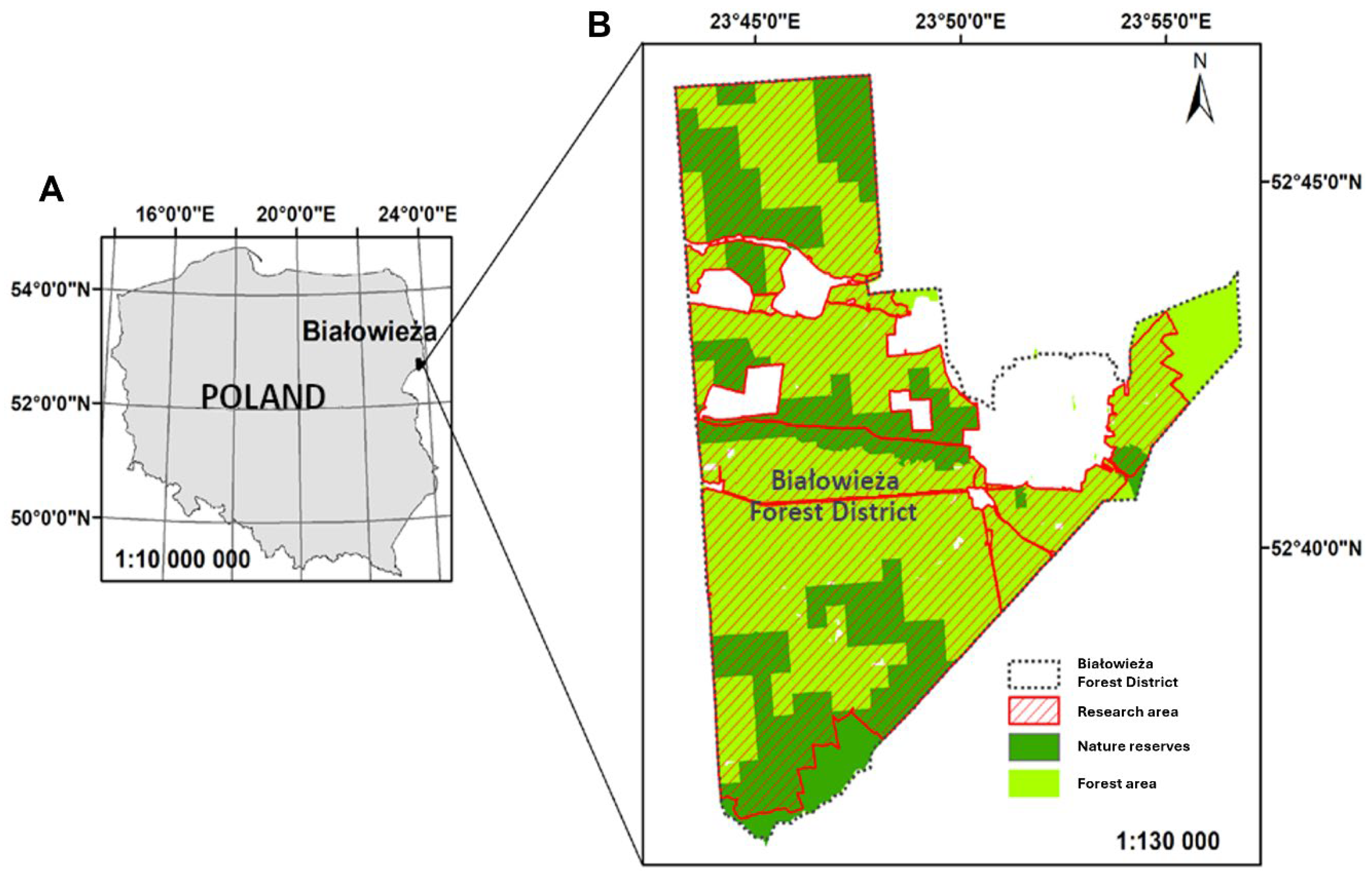
2.1. Study Area

The Białowieża Forest is an approx. 1500 km² large lowland temperate woodland located on the border of Poland and Belarus. It is one of the last old-growth, multi-species forests of Europe [59]. The Polish section of the area is managed by the Białowieża National Park and three districts of the Polish State Forest Administration: Hajnówka Forest District, Browsk Forest District, and Białowieża Forest District. This study was conducted in the Białowieża Forest District (BFD), covering approx. 103 km² [60] situated in the central part of this forest area (Figure 1).

The tree stands of the BFD are rich in species and exhibit a high degree of structural complexity. Deciduous forests cover approximately 67% of the area, dominated by black alder (Alnus glutinosa (L.) Gartn.), pedunculate oak (Quercus robur L.), hornbeam (Carpinus betulus L.), and birch (Betula spp.). In contrast, coniferous forests, primarily composed of Scots pine (Pinus sylvestris L.) and Norway spruce (Picea abies (L.) H. Karst.), account for about 33% of the forest district’s area. Over the past decade, these stands have experienced substantial structural changes due to a spruce bark beetle outbreak [53]. These changes make the BFD an ideal location for studying structural alterations, including processes related to CGs, such as their formation, overgrowth, and enlargement. Furthermore, the location of the study area in the temperate zone, together with the diverse old-growth forest ecosystems and the availability of multitemporal, high-resolution active and passive remote sensing datasets, provide an excellent testing ground for our primary hypothesis. It should be noted that due to incomplete remote sensing data coverage in 2022, the final area of interest (AOI) was limited to approximately 10,000 ha. To ensure a comparative study using data from 2015, the analysis was restricted to areas where data were acquired on both dates (Figure 1).

2.2. Data

2.2.1. Aerial Imagery

Multispectral, high-resolution aerial imagery utilised for generating point clouds and Canopy Height Models (CHMs) were collected in July 2015 and October 2022, using a large-format camera—UltraCamEagle (Vexcel Imaging/Microsoft, Graz, Austria). Data acquisitions were conducted in windless periods with cloudless weather. The radiometric resolution of the acquired photographs was 16 bits, and the spatial resolution (Ground Sampling Distance; GSD) was 0.20 m. The images were recorded in four spectral channels (R for red, G for green, B for blue, and NIR for near-infrared) with relatively high transverse (40–70%) and longitudinal (80–90%) overlap (

Table 1. Overview of the characteristics of DAP and ALS datasets.

	Aerial Imagery		Airborne Laser Scanning
Parameter	2015	2022	2015	2022
Device	UltraCam Eagle	UltraCam Eagle	Riegl LMS-Q680i	Riegl VQ-780i
Sensor type	large format RGB-NIR camera	large format RGB-NIR camera	full waveform laser scanner	full waveform laser scanner
Coverage	90/40%	80/70%	50%	20%
Flight altitude	3200 m	3960 m	500 m	900 m
Resolution/ density	0.20 m	0.20 m	11 pts/m2	38 pts/m2
Flight date	July 2015	October 2022	July 2015	October 2022

).

2.2.2. Airborne Laser Scanning Data (ALS)

Similarly to aerial imaging, airborne laser scanning (ALS) data were collected in July 2015 and October 2022. ALS point clouds were acquired using long-range airborne scanners branded by Riegl (Vienna, Austria, models: LMS-Q680i and VQ-780i). The average scanning density for each series ranged from 11 points per square metre (in 2015) to 38 points per square metre (in 2022) (Table 1).

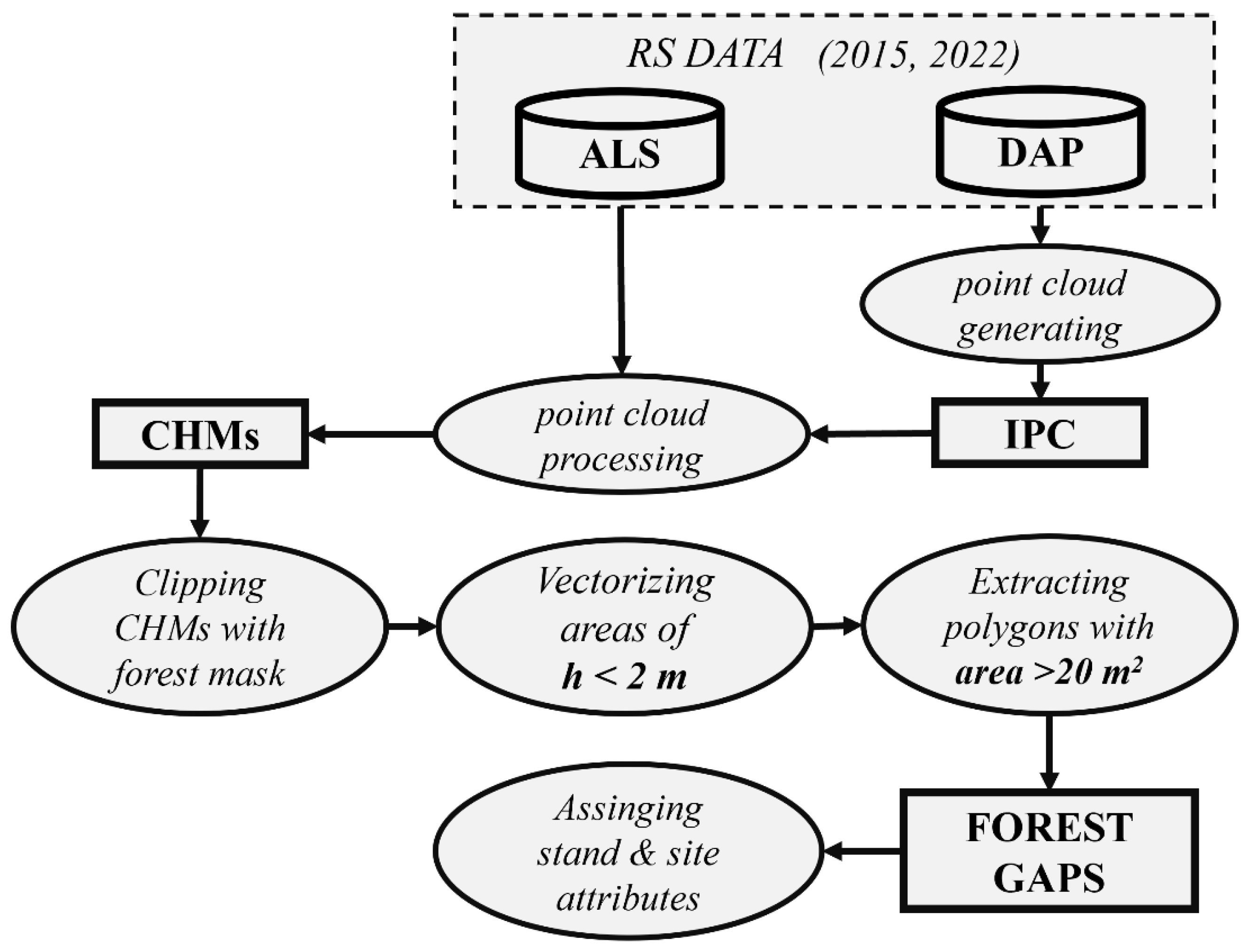
2.3. Processing of High-Resolution Aerial Imagery

Processing of aerial imagery to obtain a 3D point cloud was performed using AgiSoft PhotoScan Professional software (version 2.0) [61]. The workflow for aerial images consisted of three main steps:

(i)

The initial alignment of images was achieved through automatic aerotriangulation using a field photogrammetric warp measured in the field with a GNSS receiver. Despite automatic aerotriangulation, additional manual alignment of images was performed by application of extra photopoints and Ground Control Points (GCPs) to enhance the accuracy of the image block. Additional binding points, measured from ALS data and orthophotos, were also used in the image block alignment process.

(ii)

Dense point clouds were generated for each aerial imagery acquisition date using depth maps calculated through stereo-matching. The process of dense point cloud generation considered overlapping pairs of images, and the depth maps were combined to form a final dense point cloud, with excess information in overlapping regions that was used to filter out erroneous depth measurements.

(iii)

Digital Surface Models (DSMs) with a resolution of 0.5 m were generated from the dense point clouds for each data collection date. These models were then normalised and transformed into CHMs with a spatial resolution of 0.5 m. The normalisation process employed a Digital Terrain Model (DTM) with a resolution of 0.5 m, created from ALS data.

2.4. Processing of ALS Data

The acquired airborne laser scanning data (in LAS format) were archived in the PUWG1992 coordinate system (EPSG: 2180). ALS data were classified by the data provider according to the American Society for Photogrammetry and Remote Sensing (ASPRS) standard: 1–processed, unclassified; 2–ground; 3–low vegetation; 4–medium vegetation; 5–high vegetation; 6–buildings and engineering structures; 7–noise. Using the points classified as ground (ASPRS LAS class 2), DTMs were interpolated. Digital Surface Models (DSMs) were generated with all LiDAR points registered as first returns. The Triangular Irregular Network (TIN) interpolation was used for both digital models. The ALS data were processed using R Software 4.4.3 with the lidR package [62]. Since the point densities of the ALS datasets (11 and 38 points/m², Table 1) were both sufficient to capture key forest canopy features, the TIN model was able to produce reliable DSMs for both 2015 and 2022. The slight difference in point density between the two datasets did not significantly affect the DSM production process [63].

2.5. Gap Detection Based on Canopy Height Models

Rasters in the form of CHMs, generated from ALS data and derived from aerial imagery processing, were utilised to create vector layers representing CGs in the BFD for 2015 and 2022. Gap detection was based on the definition of a gap as an open area in a forest stand covered with vegetation of no higher than 2 m above the ground surface [6], with an area of not less than 20 m² [64].

After applying a forest mask (official product available from the Polish forestry administration), we derived a canopy gap layer by reclassifying the CHM raster with a 2 m height threshold, where all pixels with height values < 2 m were designated as gaps. These newly formed raster layers underwent a vectorization process, resulting in the creation of vector polygon layers. Following this, the next step in data processing involved the exclusion of canopy gap areas (polygons) smaller than 20 m² by applying a minimum area filter. The resulting polygon vector layers were used as the basis for further analysis. In the last step, various habitat and topographic attributes (

Table 2. Attributes assigned to polygons representing canopy gaps in the study area.

Attribute	Description
Gap area	Geometric surface area of the gap [m2]
Gap size class	Small: area ≤ 500 m2 Medium: area > 500–3000 m2 Large: area > 3000–5000 m2 Very Large: area > 5000 m2
Area of gap located in a nature reserve	Area of the gap located within nature reserve/-s [m2]
Tree species	Dominant tree species in the gap (in terms of the species’ spatial coverage). The area of the polygon covered by a given species (dominant tree species) was calculated based on information obtained from the Forest Digital Map for 2015
Gap shape index	An index determining the level of complexity of the gap shape based on the surface and perimeter of the gap, calculated according to the formula shp_index = 1/(P/(2*sqrt(A*pi)), where P = perimeter, A = gap area. The shape index takes values from 0 to 1 (the closer the index value is to 1, the less complex the gap shape—more similar to a circle)

) were calculated to characterise the identified gaps, facilitating the understanding of potential drivers that led to the CG formation within the study area (Figure 2).

2.6. Statistical Analyses

As a first step, we compared the CHMs generated by ALS and IPC methods. To facilitate this comparison, a new vector layer containing randomly distributed points (500 points) was created within the study area. Subsequently, CHM pixel values were extracted for these points. This extraction process was repeated for each CHM generated in this study. Finally, we compared the pixel values (heights) obtained from CHMs generated by different methods (i.e., ALS and IPC) for 2015 and 2022. Student’s t-test for dependent samples was applied to compare means and assess the significance of differences between heights obtained from ALS and IPC for each data acquisition date. Additionally, a correlation matrix was computed to depict the strength of correlations between heights obtained from all CHMs.

Following the implementation of the CGs detection algorithm, vector layers were produced to illustrate the size, shape, and location of CGs in the stands of the BFD for the years 2015 and 2022. These vector layers enabled the analysis of gap dynamics in the study area, focusing on CGs size and quantity. The comparison of gap detection results for the dates of data acquisition (2015 and 2022) involved overlaying the vector layers representing CGs and extracting their common parts. The CGs were categorised into three groups: (i) Newly Created: CGs present in 2022 but absent in 2015; (ii) Overgrown: CGs present in 2015 but absent in 2022; (iii) Overlapping: Intersecting CGs. For a more detailed analysis, the overlapping category was further divided into three subcategories based on the extent of overlap (%) between the area of a given CG on both data acquisition dates: (a) less than 25%, (b) 25% to 75%, and (c) more than 75%. Further, tabular summaries were generated to display the results of CG detection from the processing of ALS and IPC datasets.

To investigate CGs dynamics between 2015 and 2022 and assess the impact of bark beetle outbreak, the maps obtained from the more precise method (ALS or IPC) were utilised. The forest stands were categorised into two communities: those dominated by spruce (C1) and those dominated by other tree species (C2). The Mann–Whitney U test was employed to compare the changes in CGs between these two communities. This test was used to analyse whether the size and number of CGs increased significantly more in C1 compared to C2 as expected due to bark beetle activity in the study area. All statistical analyses were conducted using R software [65].

3. Results

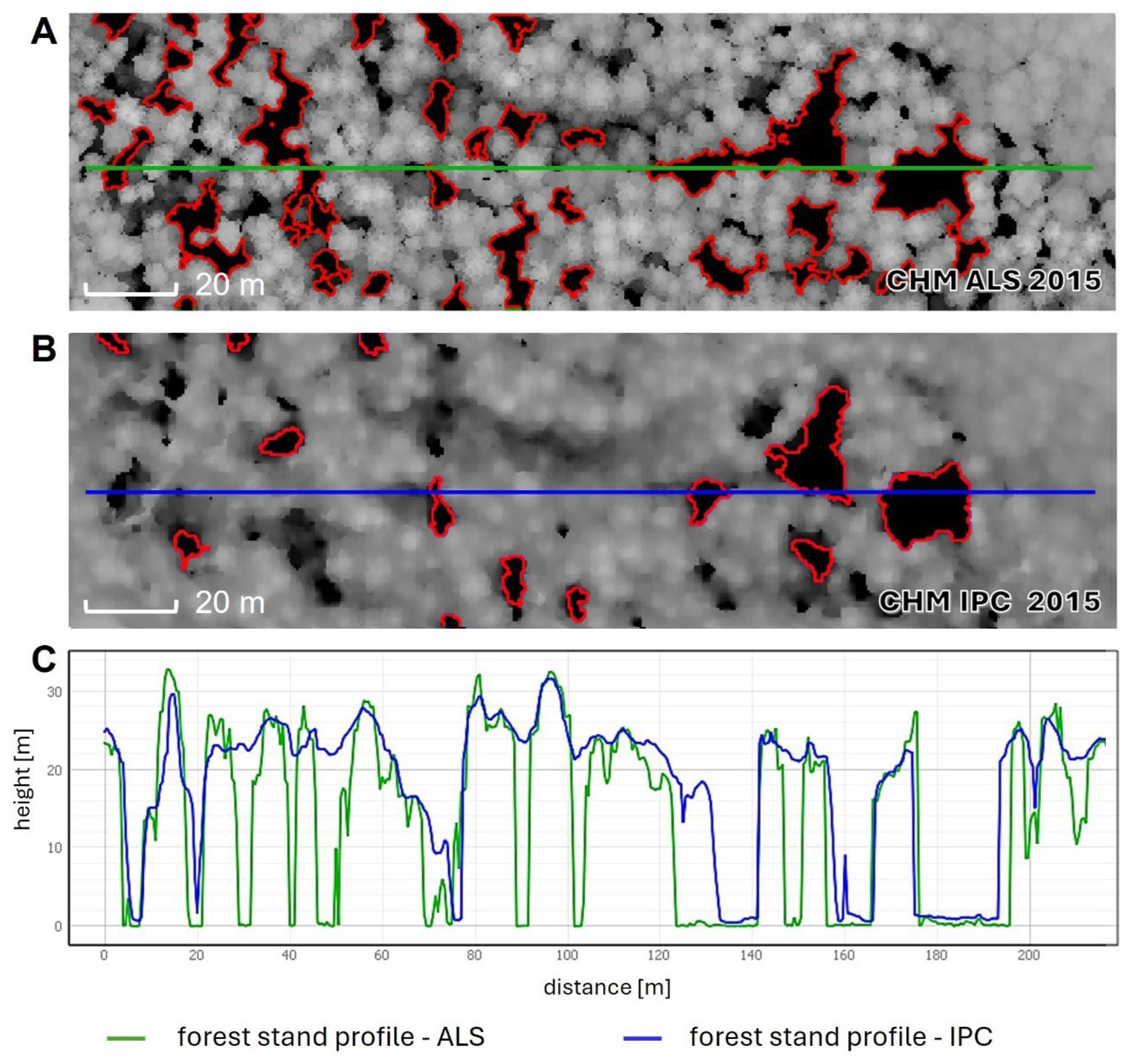
3.1. Comparison of Canopy Height Models—ALS vs. IPC

CHMs derived from ALS and IPC methods in different years of data acquisition exhibited a high degree of similarity, with mean and median values closely aligned in each respective year. The most significant average height difference between ALS and IPC occurred in 2015, amounting to 0.40 m. Minor differences were observed between the methods in 2022. It is worth mentioning that ALS-derived CHMs indicated slightly greater variability. Figure 3 shows that canopy height estimates from both IPC and ALS data are generally similar, with no significant differences between the two methods in either 2015 or 2022.

Notably, a strong positive correlation was observed between the results obtained using ALS and IPC methods. Specifically, the correlation coefficients for the same data acquisition dates were consistently high (0.97) for both years. Statistically significant differences were found between the heights derived from the two methods for the same data acquisition year. In most cases, the IPC method exhibited higher average height values compared to the ALS method.

3.2. Canopy Gaps Features—ALS vs. IPC

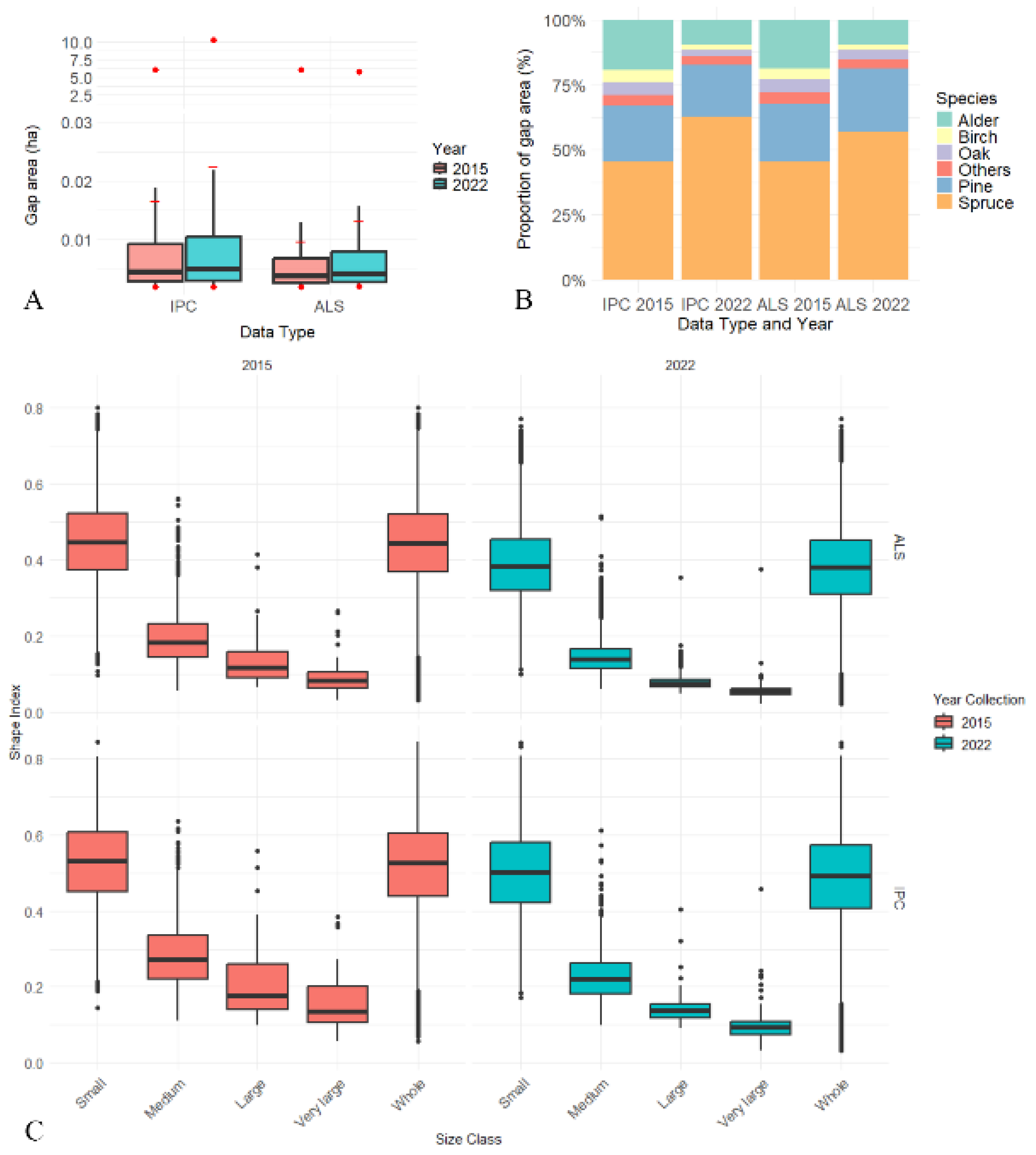
3.2.1. Gap Area

Both the average CG area (ALS: 0.010 → 0.013 ha; IPC: 0.017 → 0.022 ha) and the total CG area (ALS: 486.5 → 680.2 ha; IPC: 312.2 → 703.1 ha) increased over time across both methods. The average CG area generated by the IPC method (ranging from 0.017 ha to 0.027 ha) was larger than the value obtained using the ALS method (ranging from 0.010 ha to 0.013 ha) (Figure 4A). A significant proportion of the detected CGs (ranging from 20% to 25%, depending on the method and date of data acquisition) were situated in nature reserves.

In 2015, the area of overlapping gaps between ALS and IPC was 251.4 ha, which means that approximately 80% of the gaps detected by the IPC method (in terms of area) overlapped with those identified by the ALS method. In 2022, however, the area of overlapping forest CGs detected by the ALS and IPC methods amounted to 456.1 ha, representing nearly 70% of the CGs detected by the ALS method that overlapped with those recorded by the IPC method.

3.2.2. Dominant Tree Species vs. Spatial Distribution of Gaps

The majority of recorded CGs were situated in areas where Norway spruce was the dominant species. The total CG area in spruce stands ranged from 45% to 63% using the ALS method and from 45% to 57% for the IPC method, respectively. The total CG area in Scots pine stands was slightly lower. Among deciduous trees, black alder (10–19%), birch, and pedunculate oak (approximately 4%) had relatively high shares of the CG area. It should be noted that regardless of the method, the share of CG area by the main tree species was at a similar level in each year of data acquisition (Figure 4B).

3.2.3. Gap Shape

The IPC method generally had slightly higher shape coefficient values than the ALS method. This implies that CGs detected using the IPC method were less complex in shapes than CGs detected using the ALS method. Generally, larger CGs exhibited more complex shapes than smaller gaps. Similar trends were observed for both years and both methods (Figure 4C).

3.2.4. Distribution of Gap Size

Distribution of gap size indicated that for the ALS data, approximately half of the total area consisted of small CGs (for both data acquisition years). However, in the case of the IPC method, a larger proportion of the area was attributed to very large CGs (above 0.05 ha). The smallest percentage of the area (regardless of the method and data acquisition year) was represented by large CGs (size: 0.03–0.05 ha) (

Table 3. Total area and number of gaps in each year of data acquisition, categorised by gap size class: small (500 m² >), medium (500–3000 m²), large (3000–5000 m²), very large (>5000 m²).

	Method	Year	Gap Size Class				Total
			Small	Medium	Large	Very Large
Total area of gaps by gap size class (ha)	ALS	2015	291.92	100.54	27.41	66.64	486.50
		2022	331.59	165.47	51.41	131.72	680.20
	IPC	2015	131.20	75.85	27.28	77.90	312.22
		2022	232.49	150.00	52.24	268.33	703.06
Total number of gaps by gap size class	ALS	2015	48,755	952	71	60	49,838
		2022	49,743	1517	134	123	51,517
	IPC	2015	17,961	679	72	60	18,772
		2022	29,645	1351	135	201	31,332

). Comparing ALS and IPC methods, the most significant discrepancies were observed in the case of small CGs, where the IPC method yielded significantly lower values (Table 3).

In general, the ALS method allowed for the detection of a significantly larger number of CGs. The most pronounced difference in favour of the ALS method was particularly evident in the case of small CGs (sized 20–500 m²), with approximately 20,000 more CGs detected in 2022 and around 30,000 more in 2015. Small CGs constituted a decisive majority of all detected CGs, over 96% with the ALS method and over 93% with the IPC method. (Table 3).

The total number of CGs detected using the ALS method in individual years was relatively consistent, ranging from 49,838 (2015) to 51,517 (2022). In contrast, the cumulative numbers of CGs obtained using the IPC method were significantly more diverse, fluctuating from 18,772 (2015) to 31,332 (2022). The primary factor influencing this difference was the number of detected small CGs (Table 3).

The differences in CG detection using the ALS and IPC methods were substantial. Notably, IPC was effective in mapping crown shapes, especially discernible from a bird’s eye view (captured by a camera mounted on an aerial platform). However, challenges arose in mapping surfaces within shaded areas, specifically in areas near CG boundaries, resulting in disparities not only in the number but also in the shapes of detected CGs (Figure 5). In most instances, it was evident that the IPC method struggled to detect small CGs, while large CGs were underestimated compared to the ALS method. Additionally, the shapes of CGs identified from the IPC methods appeared more simplified and less complex (Figure 5).

3.3. Gap Dynamics from 2015 to 2022

Significant dynamics in CG distribution were observed in the study area. The number of newly created CGs during the period 2015–2022 recorded based on the ALS data was higher than for the IPC data. Notably, there is a considerable number of overgrown CGs, indicating CGs detected in 2015 that did not appear as CGs in 2022. Regarding overlapping CGs during both data acquisition dates, the number of CGs in all overlap classes was higher for the ALS data than for the IPC data (

Table 4. Gap dynamics—a comparison of the number of gaps from 2015 to 2022.

	Newly Created	Overgrown	Overlapping
			<25%	25–75%	>75%
ALS 2015–2022	27,668	22,958	6453	10,097	7299
IPC 2015–2022	23,478	9944	2653	3017	2184

).

When analysing the dynamics of CGs derived from the IPC method, a notable, almost twofold increase in both the number and area of CGs was observed in 2022 compared to 2015 (2015: 18,772 gaps; 2022: 31,332 gaps), as well as in the total area of CGs (2015: 312 ha; 2022: 703 ha). A general upward trend in both the number and area of CGs during the years of data acquisition (2015–2022) was observed. A similar trend was noted with the ALS method, where the CG area increased from 486 ha in 2015 to 680 ha in 2022 (Table 3).

Gap dynamics in the BFD included two basic scenarios: (a) the process of gap expansion, where a significant number of trees fell between 2015 and 2022, leading to a considerable increase in the CG size; and (b) the process of CG overgrowth (reduction in area and disappearance), where vegetation growth in the CGs and the expansion of the canopy contour significantly reduced one CG’s size, and another CG no longer met the definition of a CG and was absent in 2022 (Figure 6).

A Mann–Whitney U test indicated that the increase in CGs in spruce-dominated stands (C1) was statistically significantly greater than in those dominated by the other tree species (C2). Descriptive statistics further supported this finding. In community C1, the mean change in CGs was 1532.5, with a median of 468.5, and a range from −52,112.0 to 69,533.5. In comparison, community C2 had a mean change of 134.8, a median of 0.0, and a range from −57,539.2 to 57,021.8 (Figure 7). The higher mean and median in C1, as well as the wider range of values, indicate a more pronounced increase in CGs relative to C2. Overall, these findings provide robust evidence of a statistically significant and substantial increase in CGs in community C1 compared to C2 over the period from 2015 to 2022.

4. Discussion

This study provides a comparative temporal evaluation of ALS and IPC methods for analysing CG dynamics within a diverse multi-species old-growth forest with multi-layered canopy recently impacted by a spruce bark beetle outbreak. Accurate CG detection is crucial for understanding forest dynamics and supporting conservation efforts, as CGs influence regeneration, biodiversity, and overall forest health. To our knowledge, this work is one of the most comprehensive studies that assesses the efficiency of both ALS and IPC methods for CG detection in old-growth forest of the European temperate zone. In general, our findings reveal that while both methods provide reliable results, ALS achieves higher accuracy in detecting small and complex CGs. In contrast, sensitivity of IPC to factors like lighting conditions and occlusions limits its accuracy in shaded parts, particularly delineating dead standing trees within stands affected by bark beetles. Our study assesses in a comprehensive way the efficiency of advanced remote sensing technologies in forest management and monitoring, offering new insights into these methods for monitoring forest structural changes that support sustainable forest management.

4.1. Comparison of Height Information Obtained from Canopy Height Models—ALS vs. IPC

Numerous studies proved that CHMs interpolated from the ALS and IPC methods can exhibit similar properties [37,66,67,68]. It should be emphasised that both DAP and ALS data are subject to inherent sources of uncertainty that may affect the accuracy of forest structure analyses. In the case of DAP data, these uncertainties are primarily related to data processing, such as image alignment accuracy and the number and distribution of GCPs, which can introduce distortions in the IPC point cloud. For ALS data, potential errors may arise from sensor calibration issues, variations in flight altitude, scan strip overlap, or differences in point density, all of which can impact the accuracy of the derived DTM and CHM. Additionally, classification errors, particularly in ground point filtering, play a crucial role, as they directly affect the accuracy of DSM normalisation. However, the accuracy of trees/stands measurements obtained using the IPC method depends on various external factors, including atmospheric conditions, sun angle, and occlusions. These factors impact the quality of aerial photographs and, consequently, the precision of the CHM generated from the images [45,69,70]. When generating DSMs from aerial images, the IPC method utilises parallax information between different registration perspectives of the same object in various images [41]. Insufficient illumination and occlusions can impede this process, making it challenging to accurately match feature points and limiting available height information for a given area [71]. Consequently, areas covered by shadows may be inaccurately represented in the CHM, leading to errors in representing the terrain’s height and the objects on it. Due to the technical issues described above, CHMs interpolated from the IPC data present a slightly less accurate representation of tree crowns compared to their counterparts generated from the ALS data. In our study, the CHM_IPC exhibited slight smoothing compared to the CHM_ALS, which was particularly noticeable in tree species with a conical crown shape, resulting in the cutting of the treetops by IPC (Figure 5). Similar observations have been made in other studies [72,73], which highlighted challenges in mapping crown shapes using the IPC data.

The “smoothing” issue with the IPC-derived models not only affects the tops of tall trees but also impacts the height values of vegetation in low-light areas, such as vegetation in small CGs surrounded by tall trees [73]. In such situations, the height of vegetation in the CG can be artificially inflated due to interpolation, a common issue for IPCs in shaded areas [43]. Often, the lowest points used in the CHM interpolation process in shaded areas do not accurately reflect the actual (lowest) height of vegetation but rather represent vegetation that was still within the range of light (Figure 8). While the subtle underestimation of tree heights by the IPC method might not significantly impact CG detection, the overestimation of vegetation heights in CGs due to insufficient light and shadows poses a problem that can significantly distort CG detection results based on the IPC method.

Furthermore, the visual verification of points with the greatest height differences between ALS and IPC revealed that these discrepancies were partly due to a slight offset (1–2 m) between the CHMs generated by the two technologies. In some cases, points located at the tops of trees on CHM_ALS were situated in the lower parts of the crown on CHM_IPC, and vice versa. While this offset does not fundamentally impact the CGs detection process, it might have slightly distorted the results of our CHM-based vegetation height comparison. Disparities between heights obtained using the ALS and IPC method can be related to the fact that the two techniques differ in several aspects. The primary distinction lies in the technology (type of sensors) and the method of data recording. IPC is a passive remote sensing technique that records reflected light, while ALS is an active technique that emits its own light and records its reflection [34]. ALS technology can directly collect 3D data and measure the vertical structure of vegetation, whereas image-matching (stereo-matching) techniques in DAP require advanced image processing methods to produce a CHM. Furthermore, the laser beams used in ALS can penetrate tree crowns, enabling the generation of high-quality DTMs and measurements of vegetation under the canopy of a tree stand [74]. On the other hand, point clouds resulting from image processing in DAP are limited to characterising only the upper layer of tree crowns [75,76]. Therefore, a hybrid method when using IPC in forest inventories is often applied, where the IPC-generated DSM is normalised using the DTM produced from ALS [41,42,46,73,77,78].

4.2. Size, Shape, and Number of Gaps

Our results showed significant differences in the number and size of CGs detected using ALS and IPC methods, with the most significant differences observed in small CGs (Table 3). Within the group of small CGs (smaller than 500 m²), the detection issue primarily involved CGs of less than 50 m². For instance, in 2015, 31,826 CGs were detected using ALS data, whereas only 10,258 were detected using IPC. The lower efficiency of detecting small CGs with the IPC method contributes to the notable disparities in the results obtained between the two methods. This finding aligns with the results of other studies. In coastal temperate rainforests on Vancouver Island, British Columbia, Canada, CG detection results of 52,085 for ALS and 3149 for IPC, were reported. Similarly to our study, the variance in the number of detected CGs was attributed to challenges in detecting small CGs using the IPC method. The significance of addressing this issue was clearly stressed, emphasising its impact on the final results of the ALS and IPC comparison [30]. In a study from the southern boreal forest zone of Finland, difficulties in detecting small CGs with the IPC data were acknowledged, highlighting that ALS technology demonstrated much higher efficiency in mapping small-area CGs [77]. Another study, in the boreal forests of Northern Alberta, Canada, also faced the problem with detecting small CGs using IPC and, therefore, recommend using this technique only for mapping large CGs [46]. In all these studies it was generally suggested that the inferior accuracy of IPC in detecting small CGs may be due to insufficient illumination of their surfaces caused by shadows [30,46,77]. In this context, it should be emphasised that the detection of small forest CGs and the analysis of the processes occurring within them constitute a crucial element in the research on forest structure. Small-scale disturbances that create small CGs (e.g., the fall of one or a few trees) significantly contribute to the development and maintenance of the forest ecosystems [79]. Therefore, issues related to the detection of small CGs with IPC data are a significant limitation in the application of these data in CG studies.

Besides CG size, its shape also plays an important role in understanding ecological processes within the CGs [9,80]. Therefore, it is essential to focus on the accuracy of detecting CG boundaries using various methods. In this research, the shape index—a commonly used indicator in CG studies [30,81,82,83]—was employed. CGs generated from the IPC method exhibited higher shape index values, indicating less complexity (Figure 9). An analysis of the relationship between the shape index and CG size revealed that larger CGs tend to have a more intricate shape than smaller CGs. This is primarily due to the tendency of large CGs to form through the merging of several smaller CGs, resulting in a highly irregular boundary. In contrast, small CGs, formed usually by the fall of one very large or a few neighbouring trees, create compact areas with shapes more resembling ellipses. The simplification and inaccuracy of CG boundaries obtained from processing the IPC data have been noted before [30]. Hence, in line with previous studies (e.g., ref. [46]), we also emphasise that the use of the IPC method for CG detection is particularly suitable for identifying relatively large CGs with less complex shapes.

During the analysis, a problem was identified in reconstructing the shape of dead standing trees (or snags) using the DAP technique. This issue primarily affected image data acquired in 2022, a period when a significant number of spruce trees, previously attacked by bark beetles, were dead and undergoing decomposition. Reconstructing the shape of dead standing trees can be challenging for stereomatching techniques due to their specific structure and high crown openness. Dead trees often have needleless or leafless crowns, making their structure more transparent (sparse) and less uniform. As a result, the point cloud may lack the density needed to represent tree details accurately. Additionally, the problem is exacerbated by broken or fallen branches, further complicating the reconstruction process. This is especially relevant for dead spruces, which lose their smaller branches rather quickly, mainly due to weather conditions (wind, snow, etc.). This peculiarity affects the shape and structure of the trees, making the crowns more sparse and harder to map accurately using DAP techniques. Dead trees may have less distinct textures than living trees, impacting the algorithms’ ability to identify and reconstruct their structure [66]. The contrast between different parts of dead trees may also be less clear, leading to difficulties in detail identification by image processing algorithms. The consequence of the problem with the proper reconstruction of canopies and the detection of dead trees using IPC has led to the fact that CGs detected in 2022 were larger than those detected by ALS. This is particularly true for areas with sparse tree cover, where many dead trees were scattered over a wide area affected by the bark beetle outbreak (Figure 10). In these cases, where trees are isolated objects in the landscape, they are more challenging to detect and accurately reconstruct. In open areas without other objects to serve as reference points, stereomatching algorithms may struggle to determine the shape and size of a dead tree accurately. Additionally, individual trees in open areas may be surrounded by a lighter background, which, combined with the low density of their crowns, makes accurate reconstruction more difficult. Conversely, dead trees standing in groups or dense stands are usually easier to detect and reconstruct. The presence of other trees provides more contextual information and improves the quality of the point cloud by better identifying the structure and shape of the dead tree.

The described situation was certainly influenced by the quality of the point cloud obtained from the processing of aerial imagery acquired in 2022. In this case, the date and time of image acquisition negatively impacted the results: 10 October, early morning hours (7:00–10:30 am). For this latitude (52°35′E–52°50′E), at that daytime, the sun was still low on the horizon, resulting in long shadows and uneven canopy lighting, which can lead to occlusions—images are obscured, thus, objects cannot be properly reconstructed in the point cloud [66]. These occlusions cause data deficiencies in the point cloud, which may affect the quality of CHMs [37]. The low sun position also generates high contrasts between illuminated and shaded areas, complicating the process of obtaining uniform point cloud quality. This issue is particularly relevant for dead standing trees, which may have complex and irregular structures or uneven illumination and occlusions, which can lead to significant reconstruction deficiencies. Hence, it is necessary to assess the quality of the input data (focusing on sun angle analysis and the presence of shadows), before extracting CGs based on the IPC method [45]. This assessment aims to detect areas where errors may occur, such as additional gaps or underestimation of the number of CGs.

Our study area is located inside a very complex forest ecosystem in terms of stand structure and species composition [59]. The intricate structure, complexity, and composition of the forest pose considerable challenges for both ALS and IPC methods, not only in analysis but also in data processing [73]. Stands with intricate diverse tree species, elevation, and spatial structures, such as those found in the Białowieża Forest District (BFD), are particularly challenging for the IPC method [30]. The variability in vertical structure limits visibility, leading to potential loss of height information in insufficiently illuminated areas and, consequently, less accurate measurements based on the CHM generated from aerial images. ALS, on the other hand, is less susceptible to changes in tree density and crown structure. It can penetrate through tree crowns, providing information on vertical structure even in dense forests [77].

4.3. Site and Stand Factors Influencing the Spatial Distribution of Canopy Gaps

Considering the fact that around 50% of the detected CGs were located in Norway spruce-dominated stands and that the share of CGs in these communities increased in successive years of data acquisition, it is essential to note that the BFD experienced a spruce bark beetle outbreak since 2012 [84], which intensified in 2015–2017 [85]. The process of the last spruce bark beetle outbreak and the associated tree mortality during the data acquisition period (2015–2022) likely did not directly impact CG formation, given the time lag between the death of a tree and its fall [86]. However, this was not the first spruce bark beetle outbreak in our study area in recent years. Four spruce bark beetle outbreaks occurred in the BFD in the last two decades (1995, 2003, 2008, and 2012) [87]. Additionally, in March 2016, the tree felling quota for the BFD was decided to be nearly tripled [88]. According to this decision, parts of dead spruces have been felled, which might have influenced our results.

However, it is crucial to note that the calculation of the CG area covered by a specific tree species was based on spatial information extracted from the Forest Digital Map (data from 2015), representing the dominant species in the forest sub-compartments. The information does not pertain to the proportion of the dominant species in the regeneration within the CG area but rather refers to the stand present at the location of the current CG in the year of database acquisition (2015).

4.4. Gap Dynamics from 2015 to 2022

Overgrowth and the emergence of new CGs play pivotal roles in the ecological processes of natural forests [29]. Comprehensive quantitative information on CG dynamics enhances our understanding of forest disturbance and canopy dynamics and can provide important input for forest management plans [19]. Observing the dynamics of CGs by determining their spatial distribution and size in a given area across different years offers valuable insights for forest managers and other stakeholders, including nature conservationists and private landowners. Precise, multi-temporal information on canopy gap dynamics can support decision-making processes related to sustainable forest management, including the planning of both natural and artificial regeneration, as well as the monitoring of disturbance regimes. Gap dynamics are typically quantified by measuring the rate at which CGs are created and closed, as well as their lifespan [89]. In our study, the number of newly formed CGs with the ALS method in the period 2015–2022 was significantly higher than that detected with the IPC method. A more substantial difference was observed for the overgrown CGs (Table 4). These differences are likely attributed to the limited ability of the IPC method to detect small-area CGs, which are crucial for accurate CG detection [30,90].

An analysis of CGs with overlapping areas (between the years 2015 and 2022) revealed significantly more overlapping CGs with the ALS method, regardless of the percentage coverage range. This difference is likely due not only to variations in the accuracy of CG detection but also to the precision of mapping their shapes. In the ALS method, we observed more complex CG shapes, more accurately reflecting their actual boundaries. Additionally, in the IPC method, images captured at different times of the day on each data acquisition date likely influenced the presence of varying lengths and directions of shadows. Consequently, the boundaries of CGs in successive years may have been vectorized with slight shifts relative to each other.

In terms of both CG area and quantity over time, significant differences were evident between the two CGs detection techniques. The IPC method exhibited a larger area of newly created CGs and a smaller area of overgrown CGs compared to the ALS method (Table 3 and Table 4). The smaller area of overgrown CGs detected based on the IPC method, similar to the quantitative capture, might be attributed to challenges in detecting small CGs with the IPC method. Given that small CGs tend to close much faster than medium and large CGs [19], their accurate detection is crucial for analysing canopy changes between 2015 and 2022. Our study indicates that the IPC method, facing difficulties in detecting small CGs, only allows for determining general trends in CG dynamics.

The pronounced canopy disturbance in Norway spruce-dominated stands (community C1) as proven by much larger increase in CGs (Figure 7), highlights distinct spatial dynamics between the two analysed forest communities (C1 and C2) over the 2015–2022 period. The greater increase in CGs in C1 can likely be attributed to the gradual fall or cutting of dead spruce trees affected by the bark beetle outbreak since 2012 [53,60]. This ongoing tree mortality and collapse explain the more substantial canopy disruptions in spruce-dominated tree stands (C1) compared to stands dominated by the other tree species (C2).

Our results highlight the dynamic changes occurring in the stands of the BFD, with remote sensing data providing a comprehensive spatial perspective. The pronounced dynamics can be attributed to spruce bark beetle outbreaks in recent decades, resulting from various factors, e.g., drought, climate change, etc. [91]. During the last outbreak, over 0.7 million m³ of spruce and pine trees in the BFD were affected [53]. In our study, the majority of CGs were observed in areas dominated by spruce and pine (regardless of the method and date of data acquisition) (Figure 4B). Understanding the spatial and temporal patterns of gap formation, particularly in the context of increasing disturbance events (e.g., bark beetle outbreaks), can help managers prioritise areas for intervention, allocate resources more efficiently, and mitigate economic losses. These insights are particularly valuable in adapting forest policies to address the growing impacts of climate change on forest health and stability.

5. Conclusions

This study compared the effectiveness of ALS and IPC methods in analysing the vertical structure of forest ecosystems, specifically focusing on detection of CGs in a study area located in a diverse, multi-species temperate European old-growth forest recently affected by the spruce bark beetle outbreak. While both methods provided reliable altitude data, ALS proved more accurate due to its ability to generate detailed CHMs. In contrast, the IPC method, being more affected by external factors like lighting and occlusions, demonstrated constraints in detecting smaller CGs and reconstructing their shape, most likely due to its limitations in shaded areas and during times of low sun angles. A remarkable finding was the difficulty IPC faced in accurately reconstructing dead standing trees, particularly in 2022 (i.e., spruce-dominated stands), where gradual tree falls due to bark beetle infestation since 2012 likely contributed to the canopy disturbances observed over the study period.

Our study clearly highlighted the critical role of advanced remote sensing techniques, particularly ALS, in accurately detecting CGs and complex forest structure. Such methods are essential for monitoring forest dynamics and supporting sustainable forest management and nature conservation strategies. This research represents a significant step forward in advancing the application of remote sensing technologies and assessment of structurally different datasets in understanding forest CG dynamics. By revealing the strengths and limitations of each data type, it not only underscores the value and efficiency of remote sensing approaches in ecosystem conservation, forest management, and monitoring, but also enhances the understanding of forest structural changes, including those caused by bark beetle outbreaks. Future studies could explore the integration of machine learning (e.g., deep learning algorithms) to improve the accuracy and automation of canopy gap detection, particularly to enhance the identification of small gaps based on IPC data.

References

1. Kuuluvainen, T. Gap disturbance, ground microtopography, and the regeneration dynamics of boreal coniferous forests in Finland: A review. Ann. Zool. Fenn. 1994, 31, 35–51. [Google Scholar]
2. Yamamoto, S.-I. Forest gap dynamics and tree regeneration. J. For. Res. 2000, 5, 223–229. [Google Scholar] [CrossRef]
3. Dobrowolska, D. Rola luk w odnawianiu drzewostanów mieszanych w rezerwacie Jata. Sylwan 2007, 151, 14–25. [Google Scholar]
4. Bolibok, L. Regulacja Warunków Wzrostu Odnowień na Gniazdach—Wpływ Parametrów Gniazd na Oddziaływanie Czynników Biotycznych. Sylwan 2009, 153, 733–744. [Google Scholar]
5. Schliemann, S.A.; Bockheim, J.G. Methods for studying treefall gaps: A review. For. Ecol. Manag. 2011, 261, 1143–1151. [Google Scholar] [CrossRef]
6. Brokaw, N.V.L. The Definition of Treefall Gap and Its Effect on Measures of Forest Dynamics. Biotropica 1982, 14, 158–160. [Google Scholar]
7. Dobrowolska, D. Dynamika luk w drzewostanach mieszanych rezerwatu Jata. Sylwan 2006, 4, 61–75. [Google Scholar]
8. Feldmann, E.; Drößler, L.; Hauck, M.; Kucbel, S.; Pichler, V.; Leuschner, C. Canopy Gap Dynamics and Tree Understory Release in a Virgin Beech Forest, Slovakian Carpathians. For. Ecol. Manag. 2018, 415–416, 38–46. [Google Scholar] [CrossRef]
9. Muscolo, A.; Bagnato, S.; Sidari, M.; Mercurio, R. A review of the roles of forest canopy gaps. J. For. Res. 2014, 25, 725–736. [Google Scholar] [CrossRef]
10. Bonnet, S.; Gaulton, R.; Lehaire, F.; Lejeune, P. Canopy Gap Mapping from Airborne Laser Scanning: An Assessment of the Positional and Geometrical Accuracy. Remote Sens. 2015, 7, 11267–11294. [Google Scholar] [CrossRef]
11. Vilhar, U.; Roženbergar, D.; Simončič, P.; Diaci, J. Variation in irradiance, soil features and regeneration patterns in experimental forest canopy gaps. Ann. For. Sci. 2015, 72, 253–266. [Google Scholar] [CrossRef]
12. de Carvalho, L.M.T.; Fontes, M.A.L.; Oliveira-Filho, A.T. Tree Species Distribution in Canopy Gaps and Mature Forest in an Area of Cloud Forest of the Ibitipoca Range, South-Eastern Brazil. Plant Ecol. 2000, 149, 9–22. [Google Scholar] [CrossRef]
13. Wagner, S.; Fischer, H.; Huth, F. Canopy effects on vegetation caused by harvesting and regeneration treatments. Eur. J. For. Res. 2011, 130, 17–40. [Google Scholar] [CrossRef]
14. Kuijper, D.P.J.; Cromsigt, J.P.G.M.; Churski, M.; Adam, B.; Jędrzejewska, B.; Jędrzejewski, W. Do ungulates preferentially feed in forest gaps in European temperate forest? For. Ecol. Manag. 2009, 258, 1528–1535. [Google Scholar] [CrossRef]
15. Schnitzer, S.A.; Mascaro, J.; Carson, W.P. Treefall gaps and the maintenance of plant species diversity in tropical forests. In Tropical Forest Community Ecology; Carson, W.P., Schnitzer, S.A., Eds.; Blackwell Publishing: West Sussex, UK, 2008; pp. 196–209. [Google Scholar]
16. Gray, A.N.; Spies, T.A.; Pabst, R.J. Canopy Gaps Affect Long-Term Patterns of Tree Growth and Mortality in Mature and Old-Growth Forests in the Pacific Northwest. For. Ecol. Manag. 2012, 281, 111–120. [Google Scholar] [CrossRef]
17. Hammond, M.E.; Pokorný, R. Impact of Canopy Gap Ecology on the Diversity and Dynamics of Natural Regeneration in a Tropical Moist Semi-Deciduous Forest, Ghana. Biol. Life Sci. Forum 2021, 2, 10. [Google Scholar] [CrossRef]
18. Kucbel, S.; Jaloviar, P.; Saniga, M.; Vencurik, J.; Klimaš, V. Canopy gaps in an old-growth fir-beech forest remnant of Western Carpathians. Eur. J. For. Res. 2010, 129, 249–259. [Google Scholar] [CrossRef]
19. Zhu, C.; Zhu, J.; Wang, G.G.; Zheng, X.; Lu, D.; Gao, T. Dynamics of gaps and large openings in a secondary forest of Northeast China over 50 years. Ann. For. Sci. 2019, 76, 72. [Google Scholar] [CrossRef]
20. Yamamoto, S.-I.; Nishimura, N.; Torimaru, T.; Manabe, T.; Itaya, A.; Becek, K. A comparison of different survey methods for assessing gap parameters in old-growth forests. For. Ecol. Manag. 2011, 262, 886–893. [Google Scholar] [CrossRef]
21. Silva, C.A.; Valbuena, R.; Pinagé, E.R.; Mohan, M.; de Almeida, D.R.A.; Broadbent, E.N.; Jaafar, W.S.W.M.; de Almeida Papa, D.; Cardil, A.; Klauberg, C. ForestGapR: An r Package for forest gap analysis from canopy height models. Methods Ecol. Evol. 2019, 10, 1347–1356. [Google Scholar] [CrossRef]
22. Zheng, G.; Shen, G.; Moskal, L.M. Characterizing spatiotemporal variations of forest canopy gaps using aerial laser scanning data. Int. J. Appl. Earth Obs. Geoinf. 2021, 104, 102588. [Google Scholar] [CrossRef]
23. Lindenmayer, D.B.; Franklin, J.F. Conserving Forest Biodiversity: A Comprehensive Multiscaled Approach; Island Press: Washington, DC, USA, 2002. [Google Scholar] [CrossRef]
24. Diaci, J.; Adamič, T.; Rozman, A.; Fidej, G.; Roženbergar, D. Conversion of Pinus nigra Plantations with Natural Regeneration in the Slovenian Karst: The Importance of Intermediate, Gradually Formed Canopy Gaps. Forests 2019, 10, 1136. [Google Scholar] [CrossRef]
25. Runkle, J.R. Gap regeneration in some old-growth forests of the eastern United States. Ecology 1981, 62, 1041–1051. [Google Scholar] [CrossRef]
26. Yamamoto, S.-I. Gap dynamics in climax Fagus crenata forests. Bot. Mag. Shokubutsu-Gaku-Zasshi 1989, 102, 93–114. [Google Scholar] [CrossRef]
27. Dobrowolska, D.; Veblen, T.T. Treefall-Gap Structure and Regeneration in Mixed Abies alba Stands in Central Poland. For. Ecol. Manag. 2008, 255, 3469–3476. [Google Scholar] [CrossRef]
28. Itaya, A.; Miura, M.; Yamamoto, S.-I. Canopy height changes of an old-growth evergreen broad-leaved forest analyzed with digital elevation models. For. Ecol. Manag. 2004, 194, 403–411. [Google Scholar] [CrossRef]
29. St-Onge, B.; Vepakomma, U.; Sénécal, J.F.; Kneeshaw, D.; Doyon, F. Canopy gap detection and analysis with airborne laser scanning. In Forestry Applications of Airborne Laser Scanning: Concepts and Case Studies; Maltamo, M., Næsset, E., Vauhkonen, J., Eds.; Springer: Dordrecht, The Netherlands, 2013; pp. 419–437. [Google Scholar]
30. White, J.C.; Tompalski, P.; Coops, N.C.; Wulder, M.A. Comparison of airborne laser scanning and digital stereo imagery for characterizing forest canopy gaps in coastal temperate rainforests. Remote Sens. 2018, 10, 1065. [Google Scholar] [CrossRef]
31. Winstanley, P.; Dalagnol, R.; Mendiratta, S.; Braga, D.; Galvão, L.S.; Bispo, P.d.C. Post-Logging Canopy Gap Dynamics and Forest Regeneration Assessed Using Airborne LiDAR Time Series in the Brazilian Amazon with Attribution to Gap Types and Origins. Remote Sens. 2024, 16, 2319. [Google Scholar] [CrossRef]
32. Chung, C.-H.; Wang, J.; Deng, S.-L.; Huang, C. Analysis of Canopy Gaps of Coastal Broadleaf Forest Plantations in Northeast Taiwan Using UAV LiDAR and the Weibull Distribution. Remote Sens. 2022, 14, 667. [Google Scholar] [CrossRef]
33. Chen, J.; Wang, L.; Jucker, T.; Da, H.; Zhang, Z.; Hu, J.; Zhang, J. Detecting Forest Canopy Gaps Using Unoccupied Aerial Vehicle RGB Imagery in a Species-Rich Subtropical Forest. Remote Sens. Ecol. Conserv. 2023, 9, 671–686. [Google Scholar]
34. Baltsavias, E. A Comparison between Photogrammetry and Laser Scanning. ISPRS J. Photogramm. Remote Sens. 1999, 54, 83–94. [Google Scholar] [CrossRef]
35. Hyyppä, J.; Holopainen, M.; Olsson, H. Laser Scanning in Forests. Remote Sens. 2012, 4, 2919–2922. [Google Scholar] [CrossRef]
36. Wallace, L.; Lucieer, A.; Malenovský, Z.; Turner, D.; Vopěnka, P. Assessment of Forest Structure Using Two UAV Techniques: A Comparison of Airborne Laser Scanning and Structure from Motion (SfM) Point Clouds. Forests 2016, 7, 62. [Google Scholar] [CrossRef]
37. White, J.C.; Wulder, M.A.; Vastaranta, M.; Coops, N.C.; Pitt, D.; Woods, M. The utility of image-based point clouds for forest inventory: A comparison with airborne laser scanning. Forests 2013, 4, 518–536. [Google Scholar] [CrossRef]
38. Erfanifard, Y.; Stereńczak, K.; Kraszewski, B.; Kamińska, A. Development of a Robust Canopy Height Model Derived from ALS Point Clouds for Predicting Individual Crown Attributes at the Species Level. Int. J. Remote Sens. 2018, 39, 9206–9227. [Google Scholar] [CrossRef]
39. Mielcarek, M.; Stereńczak, K.; Khosravipour, A. Testing and evaluating different LiDAR-derived canopy height model generation methods for tree height estimation. Int. J. Appl. Earth Obs. Geoinf. 2018, 71, 132–143. [Google Scholar] [CrossRef]
40. Sterenczak, K.; Zasada, M.; Brach, M. The accuracy assessment of DTM generated from LIDAR data for forest area–a case study for scots pine stands in Poland. Balt. For. 2013, 19, 252–262. [Google Scholar]
41. Rahlf, J.; Breidenbach, J.; Solberg, S.; Næsset, E.; Astrup, R. Comparison of four types of 3D data for timber volume estimation. Remote Sens. Environ. 2014, 155, 325–333. [Google Scholar] [CrossRef]
42. White, J.; Stepper, C.; Tompalski, P.; Coops, N.; Wulder, M. Comparing ALS and image-based point cloud metrics and modelled forest inventory attributes in a complex coastal forest environment. Forests 2015, 6, 3704–3732. [Google Scholar] [CrossRef]
43. Goodbody, T.R.; Coops, N.C.; White, J.C. Digital Aerial Photogrammetry for Updating Area-Based Forest Inventories: A Review of Opportunities, Challenges, and Future Directions. Curr. For. Rep. 2019, 5, 55–75. [Google Scholar] [CrossRef]
44. Htun, N.M.; Owari, T.; Tsuyuki, S.; Hiroshima, T. Detecting Canopy Gaps in Uneven-Aged Mixed Forests through the Combined Use of Unmanned Aerial Vehicle Imagery and Deep Learning. Drones 2024, 8, 484. [Google Scholar] [CrossRef]
45. Zielewska-Büttner, K.; Adler, P.; Ehmann, M.; Braunisch, V. Automated detection of forest gaps in spruce dominated stands using canopy height models derived from stereo aerial imagery. Remote Sens. 2016, 8, 175. [Google Scholar] [CrossRef]
46. Dietmaier, A.; McDermid, G.J.; Rahman, M.M.; Linke, J.; Ludwig, R. Comparison of LiDAR and Digital Aerial Photogrammetry for Characterizing Canopy Openings in the Boreal Forest of Northern Alberta. Remote Sens. 2019, 11, 1919. [Google Scholar] [CrossRef]
47. Seidl, R.; Thom, D.; Kautz, M.; Martin-Benito, D.; Peltoniemi, M.; Vacchiano, G.; Wild, J.; Ascoli, D.; Petr, M.; Honkaniemi, J.; et al. Forest disturbances under climate change. Nat. Clim. Chang. 2017, 7, 395–402. [Google Scholar] [CrossRef]
48. Jaworski, T.; Hilszczański, J. The effect of temperature and humidity changes on insect development and their impact on forest ecosystems in the context of expected climate change. For. Res. Pap. 2013, 74, 345–355. [Google Scholar]
49. Wermelinger, B.; Seifert, M. Temperature-dependent reproduction of the spruce bark beetle Ips typographus, and analysis of the potential population growth. Ecol. Entomol. 1999, 24, 103–110. [Google Scholar]
50. Meddens, A.J.H.; Hicke, J.A.; Ferguson, C.A. Spatiotemporal patterns of observed bark beetle-caused tree mortality in British Columbia and the western United States. Ecol. Appl. 2012, 22, 1876–1891. [Google Scholar] [CrossRef]
51. Lausch, A.; Heurich, M.; Fahse, L. Spatio-temporal infestation patterns of Ips typographus (L.) in the Bavarian Forest National Park, Germany. Ecol. Indic. 2013, 31, 73–81. [Google Scholar] [CrossRef]
52. Hicke, J.A.; Meddens, A.J.H.; Kolden, C.A. Recent Tree Mortality in the Western United States from Bark Beetles and Forest Fires. For. Sci. 2016, 62, 141–153. [Google Scholar] [CrossRef]
53. Stereńczak, K.; Mielcarek, M.; Kamińska, A.; Kraszewski, B.; Piasecka, Ż.; Miścicki, S.; Heurich, M. Influence of selected habitat and stand factors on bark beetle Ips typographus (L.) outbreak in the Białowieża Forest. For. Ecol. Manag. 2020, 459, 117826. [Google Scholar] [CrossRef]
54. Marini, L.; Økland, B.; Jönsson, A.M.; Bentz, B.; Carroll, A.; Forster, B.; Grégoire, J.-C.; Hurling, R.; Nageleisen, L.M.; Netherer, S.; et al. Climate drivers of bark beetle outbreak dynamics in Norway spruce forests. Ecography 2017, 40, 1426–1435. [Google Scholar] [CrossRef]
55. Hlásny, T.; König, L.; Krokene, P.; Lindner, M.; Montagné-Huck, C.; Müller, J.; Qin, H.; Raffa, K.F.; Schelhaas, M.-J.; Svoboda, M.; et al. Bark Beetle Outbreaks in Europe: State of Knowledge and Ways Forward for Management. Curr. For. Rep. 2021, 7, 138–165. [Google Scholar] [CrossRef]
56. Hlásny, T.; Zimová, S.; Merganičová, K.; Štěpánek, P.; Modlinger, R.; Turčáni, M. Devastating Outbreak of Bark Beetles in the Czech Republic: Drivers, Impacts, and Management Implications. For. Ecol. Manag. 2021, 490, 119075. [Google Scholar] [CrossRef]
57. Seidl, R.; Rammer, W. Climate change amplifies the interactions between wind and bark beetle disturbances in forest landscapes. Landsc. Ecol. 2017, 32, 1485–1498. [Google Scholar] [CrossRef]
58. Abdullah, H.; Skidmore, A.K.; Darvishzadeh, R.; Heurich, M. Sentinel-2 Accurately Maps Green-Attack Stage of European Spruce Bark Beetle (Ips typographus, L.) Compared with Landsat-8. Remote Sens. Ecol. Conserv. 2019, 5, 87–106. [Google Scholar] [CrossRef]
59. Jaroszewicz, B.; Cholewińska, O.; Gutowski, J.M.; Samojlik, T.; Zimny, M.; Latałowa, M. Białowieża Forest—A Relic of the High Naturalness of European Forests. Forests 2019, 10, 849. [Google Scholar] [CrossRef]
60. Ginszt, T.; Laskowska-Ginszt, A. Ten Years (2012–2021) of Spruce Bark Beetle Ips typographus (L.) Activity in the Bialowieza Forest District of the Bialowieza Primeval Forest. Sylwan 2022, 166, 183–193. [Google Scholar] [CrossRef]
61. AgiSoft PhotoScan Professional Edition (Version 2.0) (Software). 2021. Available online: http://www.agisoft.com/downloads/installer (accessed on 11 February 2025).
62. Roussel, J.-R.; Auty, D.; Coops, N.C.; Tompalski, P.; Tristan, R.H.; Goodbody, A.; Meador, S.; Bourdon, J.-F.; Boissieu, F.; Achim, A. lidR: An R package for analysis of Airborne Laser Scanning (ALS) data. Remote Sens. Environ. 2020, 251, 112061. [Google Scholar]
63. Khosravipour, A.; Skidmore, A.K.; Isenburg, M.; Wang, T.; Hussin, Y.A. Generating pit-free canopy height models from airborne lidar. Photogramm. Eng. Remote Sens. 2014, 80, 863–872. [Google Scholar]
64. Dobrowolska, D.; Piasecka, Ż.; Kuberski, Ł.; Stereńczak, K. Canopy Gap Characteristics and Regeneration Patterns in the Białowieża Forest Based on Remote Sensing Data and Field Measurements. For. Ecol. Manag. 2022, 511, 120123. [Google Scholar] [CrossRef]
65. R Core Team. R: A Language and Environment for Statistical Computing; R Foundation for Statistical Computing: Vienna, Austria, 2023; Available online: https://www.R-project.org/ (accessed on 20 July 2024).
66. Baltsavias, E.; Gruen, A.; Eisenbeiss, H.; Zhang, L.; Waser, L.T. High-Quality Image Matching and Automated Generation of 3D Tree Models. Int. J. Remote Sens. 2008, 29, 1243–1259. [Google Scholar] [CrossRef]
67. St-Onge, B.; Vega, C.; Fournier, R.A.; Hu, Y. Mapping canopy height using a combination of digital stereo-photogrammetry and lidar. Int. J. Remote Sens. 2008, 29, 3343–3364. [Google Scholar] [CrossRef]
68. Straub, C.; Stepper, C.; Seitz, R.; Waser, L.T. Potential of UltraCamX stereo images for estimating timber volume and basal area at the plot level in mixed European forests. Can. J. For. Res. 2013, 43, 731–741. [Google Scholar] [CrossRef]
69. Vepakomma, U.; St-Onge, B.; Kneeshaw, D. Spatially explicit characterization of boreal forest gap dynamics using multi-temporal lidar data. Remote Sens. Environ. 2007, 112, 2326–2340. [Google Scholar] [CrossRef]
70. Vepakomma, U.; St-Onge, B.; Kneeshaw, D. Response of a boreal forest to canopy opening: Assessing vertical and lateral tree growth with multi-temporal lidar data. Ecol. Appl. 2011, 21, 99–121. [Google Scholar] [CrossRef]
71. Holopainen, M.; Vastaranta, M.; Karjalainen, M.; Karila, K.; Kaasalainen, S.; Honkavaara, E.; Hyyppa, J. Forest Inventory Attribute Estimation Using Airborne Laser Scanning, Aerial Stereo Imagery, Radargrammetry and Interferometry—Finnish Experiences of the 3D Techniques. ISPRS Ann. Photogramm. Remote Sens. Spat. Inf. Sci. 2015, II–3/W4, 63–69. [Google Scholar] [CrossRef]
72. Heurich, M.; Schadeck, S.; Weinacker, H.; Krzystek, P. Forest Parameter Derivation from DTM/DSM Generated from LiDAR and Digital Modular Camera (DMC). Int. Arch. Photogramm. Remote Sens. Spat. Inf. Sci. 2004, XXXV, 84–89. [Google Scholar]
73. Mielcarek, M.; Kamińska, A.; Stereńczak, K. Digital aerial photogrammetry (DAP) and airborne laser scanning (ALS) as sources of information about tree height: Comparisons of the accuracy of remote sensing methods for tree height estimation. Remote Sens. 2020, 12, 1808. [Google Scholar] [CrossRef]
74. Petzold, B.; Reiss, P.; Stössel, W. Laser scanning—Surveying and mapping agencies are using a new technique for the derivation of digital terrain models. ISPRS J. Photogramm. Remote Sens. 1999, 54, 95–104. [Google Scholar] [CrossRef]
75. Rahlf, J. Forest Resource Mapping Using 3D Remote Sensing: Combining National Forest Inventory Data and Digital Aerial Photogrammetry; Norwegian University of Life Sciences: Ås, Norway, 2017. [Google Scholar]
76. Fassnacht, F.E.; White, J.C.; Wulder, M.A.; Næsset, E. Remote Sensing in Forestry: Current Challenges, Considerations, and Directions. Forestry 2024, 97, 11–37. [Google Scholar] [CrossRef]
77. Vastaranta, M.; Wulder, M.A.; White, J.C.; Pekkarinen, A.; Tuominen, S.; Ginzler, C.; Kankare, V.; Holopainen, M.; Hyyppä, J.; Hyyppä, H. Airborne laser scanning and digital stereo imagery measures of forest structure: Comparative results and implications to forest mapping and inventory update. Can. J. Remote Sens. 2013, 39, 382–395. [Google Scholar] [CrossRef]
78. St-Onge, B.; Audet, F.-A.; Bégin, J. Characterizing the height structure and composition of a boreal forest using an individual tree crown approach applied to photogrammetric point clouds. Forests 2015, 6, 3899–3922. [Google Scholar] [CrossRef]
79. Lertzman, K.P.; Sutherland, G.D.; Inselberg, A.; Saunders, S.C. Canopy gaps and the landscape mosaic in a coastal temperate rain forest. Ecology 1996, 77, 1254–1270. [Google Scholar] [CrossRef]
80. Seidel, D.; Ammer, C.; Puettmann, K. Describing forest canopy gaps efficiently, accurately, and objectively: New prospects through the use of terrestrial laser scanning. Agric. For. Meteorol. 2015, 213, 23–32. [Google Scholar] [CrossRef]
81. Hu, L.; Zhu, J. Determination of the Tridimensional Shape of Canopy Gaps Using Two Hemispherical Photographs. Agric. For. Meteorol. 2009, 149, 862–872. [Google Scholar] [CrossRef]
82. Koukoulas, S.; Blackburn, G.A. Spatial relationships between tree species and gap characteristics in broad-leaved deciduous woodland. J. Veg. Sci. 2005, 16, 587–596. [Google Scholar] [CrossRef]
83. Rodes-Blanco, M.; Ruiz-Benito, P.; Silva, C.A.; García, M. Canopy gap patterns in Mediterranean forests: A spatio-temporal characterization using airborne LiDAR data. Landsc. Ecol. 2023, 38, 3427–3442. [Google Scholar] [CrossRef]
84. Brzeziecki, B.; Hilszczański, J.; Kowalski, T.; Łakomy, P.; Małek, S.; Miścicki, S.; Modrzyński, J.; Sowa, J.; Starzyk, J. Problem Masowego Zamierania Drzewostanów Świerkowych w Leśnym Kompleksie Promocyjnym “Puszcza Białowieska”. Sylwan 2018, 162, 373–386. [Google Scholar] [CrossRef]
85. Erfanifard, Y.; Lisiewicz, M.; Stereńczak, K. High-Resolution Remote Sensing for Biodiversity Assessment and Monitoring: A Case Study of Dominant Tree Species in an Old-Growth Forest. For. Ecol. Manag. 2024, 566, 122094. [Google Scholar] [CrossRef]
86. Storaunet, K.O.; Rolstad, J. Time since death and fall of Norway spruce logs in old-growth and selectively cut boreal forest. Can. J. For. Res. 2002, 32, 1801–1812. [Google Scholar] [CrossRef]
87. Grodzki, W. Gradacyjne Występowanie Kornika Drukarza Ips typographus (L.) (Col.: Curculionidae, Scolytinae) w Aspekcie Kontrowersji Wokół Puszczy Białowieskiej. Leśne Pr. Badaw. 2016, 77, 324–331. [Google Scholar] [CrossRef]
88. Krzywicka, A. Ochrona przyrody i gospodarka leśna w Puszczy Białowieskiej: Brak kompleksowej strategii działania. Kontrola Państwowa 2020, 65, 33–44. [Google Scholar]
89. Vepakomma, U.; Kneeshaw, D.; Fortin, M.-J. Spatial contiguity and continuity of canopy gaps in mixed wood boreal forests: Persistence, expansion, shrinkage and displacement. J. Ecol. 2012, 100, 1257–1268. [Google Scholar] [CrossRef]
90. Ali-Sisto, D.; Packalen, P. Forest Change Detection by Using Point Clouds from Dense Image Matching Together with a LiDAR-Derived Terrain Model. IEEE J. Sel. Top. Appl. Earth Obs. Remote Sens. 2016, 10, 1197–1206. [Google Scholar] [CrossRef]
91. Gutowski, J.M.; Jaroszewicz, B. Zmiany Udziału Świerka Pospolitego w Drzewostanach Puszczy Białowieskiej w Kontekście Dynamiki Liczebności Kornika Drukarza Ips typographus (L.). In Stan Ekosystemów Leśnych Puszczy Białowieskiej; Wikło, A., Ed.; CILP: Warszawa, Poland, 2016; pp. 87–108. [Google Scholar]
Figure 1. Location of Białowieża Forest (A) and extent of the study area (B).
Remotesensing 17 01149 g001
Figure 2. Simplified data processing scheme.
Remotesensing 17 01149 g002
Figure 3. Descriptive statistics of heights from image (IPC)- and aerial laser scanning (ALS)-based canopy height models (CHMs) for each year (2015, 2022), analysed with paired t-tests (Similar letters indicate no significant difference at α = 0.05) for 500 randomly distributed points.
Remotesensing 17 01149 g003
Figure 4. A comprehensive overview of the canopy gap characteristics in the Białowieża Forest District obtained from image-derived (IPC) and aerial laser scanning (ALS) point clouds. A summary of canopy gap statistics for the time frame (2015, 2022), contrasting the ALS and IPC (red dashes and dots show mean values and data range, respectively) (A); the share (%) of gap area considering the dominant tree species in each stand based on the Forest Digital Map (B), and the average values of gap shape index calculated for each year and categorised by gap size classes (small ≤ 500 m2, medium > 500–3000 m2, large > 3000–5000 m2, very large > 5000 m2) (C).
Remotesensing 17 01149 g004
Figure 5. Comparison of gap detection in CHMs generated using the ALS (A) and IPC (B) methods for the year 2015, along with the corresponding height profile (C).
Remotesensing 17 01149 g005
Figure 6. The visualisation of the processes of enlargement (AC) and overgrowth (DF) of a canopy gap between 2015 (green polygons) and 2022 (blue polygons).
Remotesensing 17 01149 g006
Figure 7. Comparison of mean change in canopy gap area for communities C1 (dominated by Norway spruce) and C2 (dominated by the other tree species) in the period 2015–2022.
Remotesensing 17 01149 g007
Figure 8. The effect of the “tree top cutting” and false overestimation of vegetation height in gaps in the CG detection method based on the DAP technology: (A) CHM_ALS, (B) CHM_IPC, and (C) the corresponding height profiles.
Remotesensing 17 01149 g008
Figure 9. Comparison of the shape and size of canopy gaps in the same section of the study area vectorized from the ALS (A) and the IPC data (B) for 2015, showing how the IPC method simplifies the shape of gaps and underestimates their area.
Remotesensing 17 01149 g009
Figure 10. Challenges in the accurate reconstruction and segmentation of dead standing trees (snags) using IPC in 2022. Panels (AC) show a fragment of study area in 2015, when no dead trees were present, and canopy gaps were properly delineated. Panels (DF) illustrate the same area in 2022, where the presence of snags led to inaccuracies in their detection and delineation.
Remotesensing 17 01149 g010