Investigating Source Mechanisms for Nonlinear Displacement of GNSS Using Environmental Loads

Abstract

Global surface pressure, terrestrial water storage models, and seabed pressure grids provide valuable support for studying the mechanisms of the nonlinear motion behind GNSS stations. These data allow for the precise identification and analysis of displacement effects caused by environmental loads. This study analyzes GNSS coordinate time series data from 186 ITRF reference stations worldwide over a 10-year period, thoroughly examining the magnitude, spatial distribution, and impact of hydrological, atmospheric, and non-tidal oceanic loading on nonlinear motion. The results indicate that the atmospheric loading effects had a magnitude of approximately ±5 mm in the up (U) direction and ±1 mm in the east (E) and north (N) directions. Moreover, the impact of atmospheric loading on station displacements was more pronounced in high-latitude regions compared with mid- and low-latitude regions. Secondly, the hydrological loading showed a magnitude of approximately ±5 mm in the U direction and ±0.8 mm in the E and N directions, with inland areas causing larger displacements than coastal regions. Furthermore, the non-tidal oceanic loading induced displacements with magnitudes of approximately ±0.5 mm in the E and N directions and ±2 mm in the U direction, significantly affecting stations in the nearshore areas more than inland stations. Subsequently, this study analyzes the corrective effects of environmental loads on the coordinate time series. The average correlation coefficients between the E, N, and U directions and the coordinate time series were 0.35, 0.31, and 0.52, respectively. After removing the displacements caused by environmental loads, the root mean square (RMS) values of the coordinate time series decreased by 85.5% in the E direction, 77.4% in the N direction, and 89.8% in the U direction, with average reductions of 6.2%, 4.4%, and 16.7%, respectively. Lastly, it also comprehensively assesses the consistency between environmental loads and coordinate time series from the perspectives of the optimal noise model, velocity and uncertainty, and amplitude and phase. This study demonstrates that the geographic location of a station is closely related to the impact of environmental loads, with a significantly greater effect in the vertical direction than that in the horizontal direction. By correcting for environmental loads, the accuracy of the coordinate time series can be significantly enhanced.

1. Introduction

The GNSS coordinate time series contains valuable data, reflecting not just the long-term linear trends of stations but also capturing nonlinear variations arising from factors like imperfect models, geophysical effects, and unmodeled variables [1,2,3]. In order to obtain accurate position and velocity information for a station, it is necessary to quantitatively analyze different factors which affect the displacement of the station so as to deeply explore the physical mechanism of the nonlinear motion of the station and provide support for improving the error model [4,5,6,7,8,9]. Therefore, it is of great theoretical and practical value to study the signal source mechanism which causes the nonlinear movement of GNSS reference stations [10].

The movement of GNSS reference stations exhibits significant seasonal variations. Environmental loading effects, stemming from the redistribution of surface mass, constitute the primary factor contributing to the nonlinear changes observed in GNSS coordinate time series. These effects predominantly encompass atmospheric loading, hydrological loading, and non-tidal ocean loading [4,11,12,13]. Both domestic and international scholars have conducted extensive research on the displacements induced by environmental loading effects, yielding abundant findings. Dong et al. (2002) [4] conducted an analysis of the displacement induced by environmental loading effects across 36 GNSS stations worldwide. Their findings indicated that atmospheric, non-tidal ocean, and hydrological loading could collectively account for nearly half of the vertical seasonal variation [4]. The impact of non-tidal ocean loading on the vertical displacement of GNSS stations was investigated by van Dam et al. (2012) [14]. Their results revealed that the root mean square (RMS) ranged between 0.2 mm and 3.7 mm, which is more than two times smaller than the displacement caused by atmospheric loading [14]. Jiang et al. (2013) [13] conducted a comparative analysis of various environmental loading models’ influence on vertical coordinate time series based on data from 233 measurement stations worldwide. Their findings indicated that, on average, the vertical weighted root mean square (WRMS) value was reduced by 41–71% [13]. Xu et al. (2017) discovered that under optimal conditions, three environmental loading effects could account for approximately 50% of the vertical annual amplitude of GNSS reference stations [15]. The dispersion of vertical coordinate time series from the reference stations of the Crustal Movement Observation Network of China (CMONOC) sees a reduction of up to 24% following atmospheric loading correction [16]. Additionally, due to the impact of other environmental factors like wind and ocean circulation, significant regional disparities exist in the influence of non-tidal ocean loading (NTOL) on coastal GNSS stations [17]. Li et al. (2020) conducted an assessment and validation of the impact of surface pressure data with varying spatial and temporal resolutions globally on rectifying nonlinear changes in the elevation time series of ITRF2014 frame points [10]. Gobron et al. (2021) analyzed the vertical motion of over 10,000 stations worldwide and observed that correcting for non-tidal atmospheric and ocean loading could decrease the uncertainty of GNSS station vertical coordinate time series by 70% in high-latitude regions [7]. Niu et al. (2022) conducted a consistency analysis between the displacement of environmental loading and the periodicity of GNSS coordinate time series, and the results showed that environmental loading effects could explain 43% of the vertical coordinate time series but less than 20% of the horizontal component [18].

In conclusion, there exists a strong correlation between the seasonal fluctuations observed in GNSS reference stations and environmental loading effects [19,20]. However, current research on the displacement consistency of stations and environmental loading effects mainly focuses on the effect in the vertical direction [21,22,23]. Only a few studies have analyzed the consistency of horizontal seasonal variations in specific regions [15,24], and studies often lack comprehensive analyses of noise characteristics [25]. As for the comprehensive analysis of the overall nonlinear motion of GNSS coordinate time series due to environmental loading in the east, north, and up components of global IGS reference stations, research is limited [18,26].

The main purpose of this study is to analyze the signal response mechanism of the nonlinear movement of GNSS reference stations from the perspective of environmental load, deeply analyze the magnitude and spatiotemporal distribution characteristics of the displacement caused by environmental loading effects, determine the quantitative relationship between environmental loading effects and the noise, velocity, amplitude, and phase of the reference station, and reveal the essential characteristics of seasonal deformation of GNSS coordinate time series. It provides a reference for obtaining more accurate and reliable geodetic data. The structure of this article is as follows: Firstly, it introduces the data sources and calculation process. Then, it quantitatively analyzes the spatiotemporal distribution of environmental loading effects and further investigates its relationship with GNSS coordinate time series. Additionally, it delves into the changes in GNSS coordinate time series after correcting environmental loading effects. Finally, it discusses and summarizes the corresponding results.

2. Data Source and Processing Strategy

2.1. IGS Repro2 Coordinate Residuals

The GNSS coordinate time series were obtained from the second reprocessing campaign conducted by the International GNSS Service (IGS) Analysis Center within the ITRF2014 framework. Through the application of cutting-edge models and methodologies, the global GNSS station data spanning from 1994 to 2014 underwent rigorous reanalysis, resulting in enhanced precision and accuracy [27]. The preprocessing of the coordinate time series involved the systematic removal of linear trends, outliers, post-seismic deformation, and offsets, and the data retained deformations induced by unmodeled surface mass loading as well as unmodeled seasonal systematic errors.

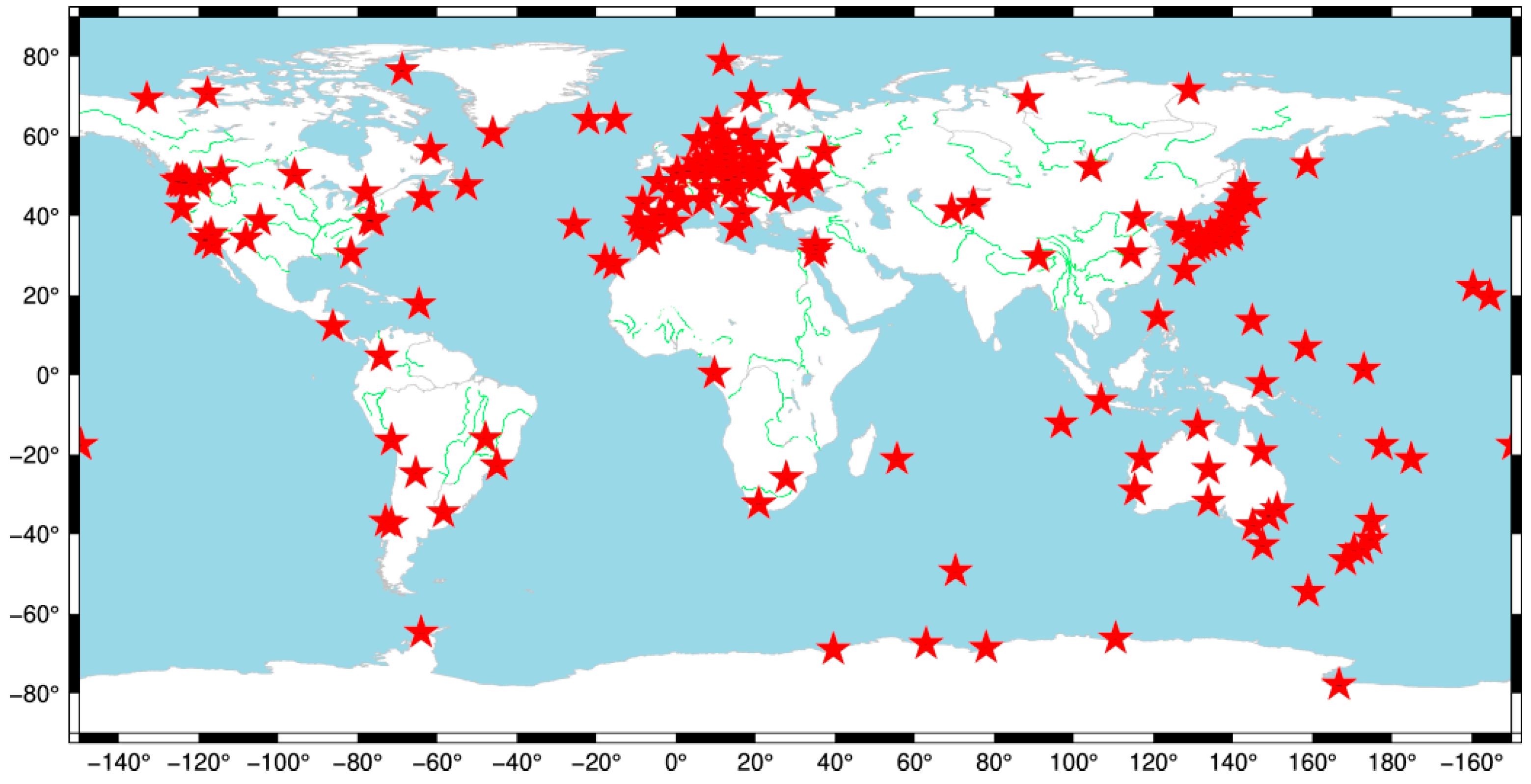
To conduct a more scientifically rigorous and reliable analysis of the nonlinear motion source mechanism within GNSS coordinate time series, it is imperative to meticulously select benchmark stations characterized by extended time spans, exceptional data quality, and a globally uniform distribution to serve as experimental sites. Stations with low data integrity (<90%) or with a short time span (<8 years) were excluded in this study. Ultimately, 186 stations distributed globally were chosen, each providing a decade-long coordinate time series, with an average data completeness rate of 95.8%, as illustrated in Figure 1.

2.2. Environmental Loading Effects

Changes in the mass of the Earth’s surface, such as in the atmosphere and water, lead to the Earth’s elastic loading response, which is mainly manifested as seasonal surface displacement. It mainly includes atmospheric mass loading (ATML), non-tidal ocean loading (NTOL), and hydrological loading (HYDL). The solid Earth’s response to surface mass loading is generally calculated using loading Green’s functions or spherical harmonic functions. The method using loading Green’s functions primarily considers the effects of higher-order spherical harmonic coefficients, while the method using spherical harmonic functions initially considers the effects of lower-order coefficients. Mathematically, the two approaches are equivalent; under identical loading conditions, the precision of the displacement computed at any single surface point is consistent between the methods, both in terms of error levels and computational efficiency.

The global surface fluid mass loading can be expanded as the sum of the spherical harmonics of the associated Legendre functions as follows:

$$h_w={\displaystyle \sum _{n=0}^{N_{\max }}{\displaystyle \sum _{m=0}^n(\Delta Q_{nm}^h\cos m\lambda +\Delta T_{nm}^h\sin m\lambda )}}{\overline{P}}_{nm}(\cos \theta )$$

(1)

where $h_w(\theta ,\lambda )$ is the equivalent water column height, $\theta$ and $\lambda$ represent the latitude and longitude of the point, respectively, $\Delta Q_{nm}^h$ and $\Delta T_{nm}^h$ refer to the spherical harmonic coefficients for the global surface loading expanded in terms of the equivalent water column height, ${\overline{P}}_{nm}$ is the $4\pi$ normalized associated Legendre function, $n$ and $m$ denote the order and degree, respectfully, and $N_{\max }$ represents the maximum truncation degree associated with spatial resolution.

According to the definition of loading love numbers, the convolution formula of Green’s function in a station-centered coordinate system can be obtained to calculate the surface displacement in the east, north, and up components caused by mass loading [28]:

$$E={\displaystyle {\int }_0^{2\pi }d{\lambda }^{\prime }}{\displaystyle {\int }_0^{\pi }{\tau }_e{\rho }_w{h}_w}({\displaystyle \frac{R}{M}}{\displaystyle \sum _{n=0}^{\infty }{l}_n^{\prime }}{\displaystyle \frac{\partial }{\partial \theta }}{P}_n(\cos \psi ))R^2\sin {\theta }^{\prime }d{\theta }^{\prime }$$

(2)

$$N={\displaystyle {\int }_0^{2\pi }d{\lambda }^{\prime }}{\displaystyle {\int }_0^{\pi }{\tau }_n{\rho }_w{h}_w}({\displaystyle \frac{R}{M}}{\displaystyle \sum _{n=0}^{\infty }{l}_n^{\prime }}{\displaystyle \frac{\partial }{\partial \theta }}{P}_n(\cos \psi ))R^2\sin {\theta }^{\prime }d{\theta }^{\prime }$$

(3)

$$U={\displaystyle {\int }_0^{2\pi }d{\lambda }^{\prime }}{\displaystyle {\int }_0^{\pi }{\rho }_w{h}_w}({\displaystyle \frac{R}{M}}{\displaystyle \sum _{n=0}^{\infty }{h}_n^{\prime }}{P}_n(\cos \psi ))R^2\sin {\theta }^{\prime }d{\theta }^{\prime }$$

(4)

where ${\rho }_w$ is the water density, $R$ is the mean radius of the Earth, ${\theta }^{\prime }$ and ${\lambda }^{\prime }$ denote the latitude and longitude, $P_n$ represents the Legendre function, and $h_n^{\prime }$ and $l_n^{\prime }$ indicate the loading love numbers. The comprehensive derivation process is presented in Farrell’s work [28], which can be consulted for further reference.

Three-dimensional displacements caused by ATML were generated using the National Centers for Environmental Prediction’s (NCEP, https://www.weather.gov/ncep/, accessed on 23 January 2025) 6-hourly surface pressure grids, which are 2.5° × 2.5° in longitude and latitude [29]. The HYDL surface displacements were derived from the terrestrial water storage model, which is provided by the Global Land Data Assimilation System (GLDAS, https://ldas.gsfc.nasa.gov/gldas, accessed on 23 January 2025) [30], with a temporal resolution of 3 h and a spatial resolution of 1° × 1°. It includes data on snow depth, soil moisture, precipitation, lakes, rivers, and more. The NTOL model utilizes data derived from the Estimating the Circulation & Climate of the Ocean (ECCO) project, provided by the National Oceanographic Partnership Program (NOPP, https://www.boem.gov/environment/environmental-studies/national-oceanographic-partnership-program, accessed on 23 January 2025) [31]. It has a temporal resolution of 12 h and a spatial resolution of 1° × (0.3°~1°). The temporal resolution of the environmental loading effects was averaged to a resolution of 1 day.

3. Spatial and Temporal Distributions of Environmental Loading Effect Displacements

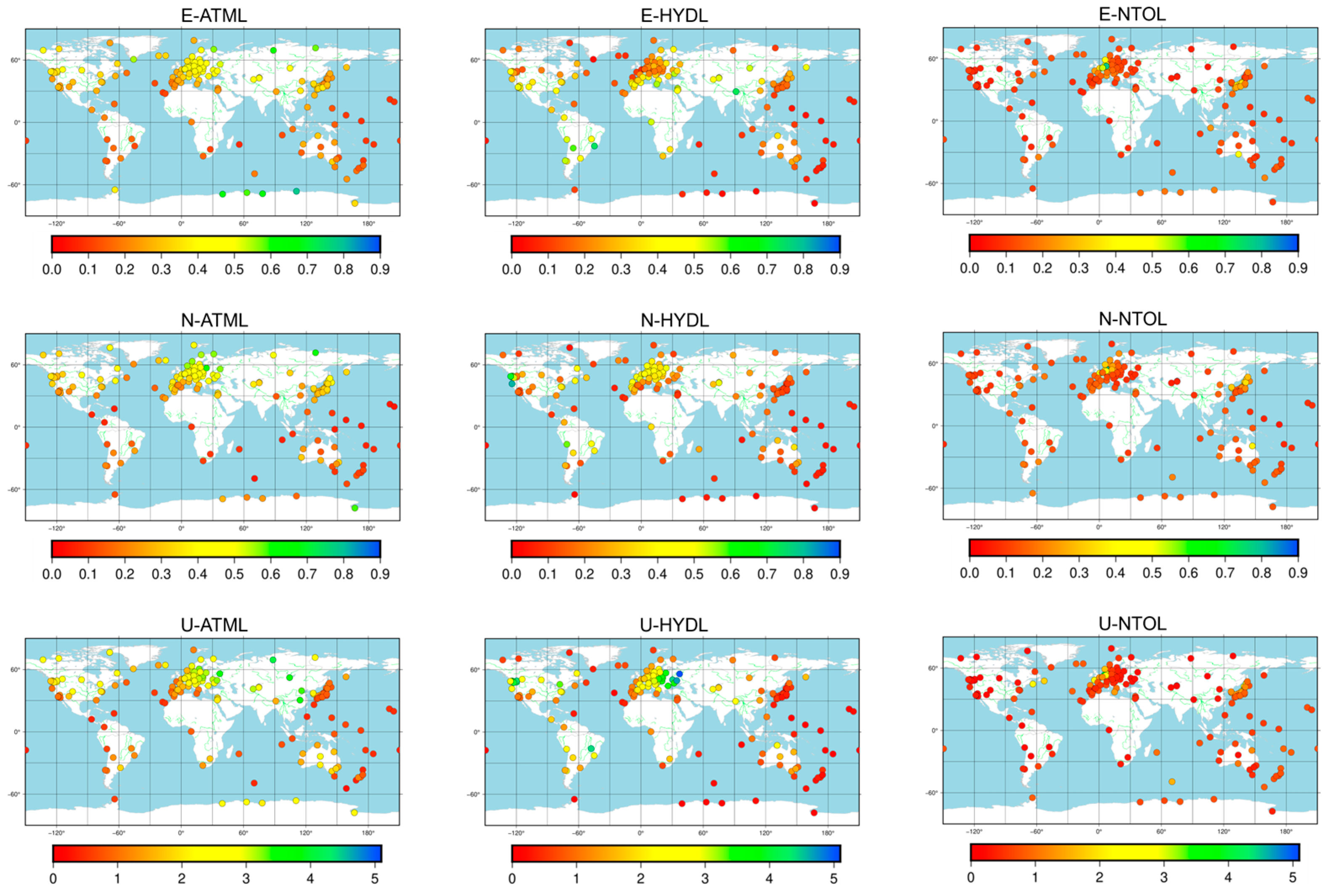
Initially, a quantitative analysis of displacement resulting from environmental loading effects, taking into account both geographical distribution and data characteristics, was conducted. As shown in Figure 2, the effects of environmental loads such as ATML, HYDL, and NTOL are related to station locations, with particularly pronounced deformation effects observed in the up components.

The influence of ATML on the U components was primarily within a range of ±5 mm, while its effect on the E and N components was mainly within a range of ±1 mm. As illustrated in the figure, there was a noticeable correlation between ATML and the latitude of the station. With increasing latitude, the displacement caused by atmospheric loading tended to increase, especially in the mid-to-high-latitude regions, where its impact was significant. In contrast, the impact in low-latitude regions was relatively minor. The analysis suggests that the displacement induced by atmospheric loading is a direct expression of the pressure changes acting on the solid Earth. Therefore, stations in high-latitude regions are more affected by atmospheric loading, while those in low-latitude regions are less affected. Consequently, this leads to differences in the influence of atmospheric loading effects across high, middle, and low latitudes. Moreover, variations exist in the magnitude of displacement caused by atmospheric loading effects between the Northern and Southern Hemispheres, possibly due to differences in atmospheric pressure zones resulting from disparities in land-sea distribution.

The HYDL primarily induced fluctuations of about ±5 mm in the U component and ±0.8 mm in the E and N components. The hydrological loading effect is primarily associated with variations in soil moisture and snow cover. Generally, displacement induced by hydrological loading is greater in inland areas compared with coastal regions.

The magnitude of the NTOL was primarily within ±2 mm in the U component and ±0.5 mm in the E and N components. Displacements caused by non-tidal ocean loading are primarily influenced by the station’s local environment. The coastline is a critical geographic feature which significantly influences the response of GNSS coordinate time series to NTOL. Generally, the effect of NTOL on stations in coastal areas is more significant than on those in inland regions. GNSS stations located near the coastline are typically more affected by NTOL as ocean mass variations—such as sea level changes and ocean currents—directly impact the coastal crust, leading to surface deformation. However, due to the varying marine characteristics of coastal areas, the impact of NTOL also shows significant differences. For example, stations in the near-coastal regions of the Atlantic Ocean and the Sea of Japan are more strongly influenced by NTOL due to active atmospheric circulation compared with other coastal areas. With respect to mountains, this study suggests that the impact of NTOL is minimal in inland areas, and no significant effect is observed in mountainous regions.

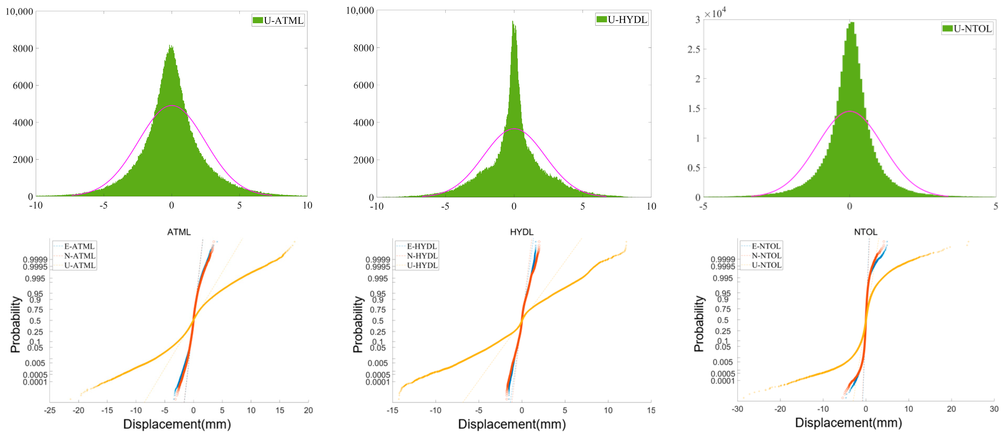
Figure 3 shows the normal distributions and normalization of data for 186 global GNSS stations in the E, N, and U directions under the effects of ATML, HYDL, and NTOL. Each direction’s distribution closely follows a normal distribution, as evidenced by the Gaussian fits shown in pink, suggesting that the majority of displacement values are centered around zero. However, the magnitudes of displacement differ significantly across the three loading types. The atmospheric and hydrological loadings exhibit larger magnitudes of influence compared with non-tidal ocean loading. The cumulative plots reveal that the atmospheric and hydrological loadings tend to cause more extreme displacement values (both positive and negative) in the vertical direction (U) compared with the horizontal directions. The non-tidal oceanic loading shows a narrower range of displacement values. Detailed percentages of the normal distribution can be found in

Table 1. Percentile proportion of normal distribution of displacement caused by ATML, HYDL, and NTOL.

Load	E (/mm)		N (/mm)		U (/mm)
	5%	95%	5%	95%	5%	95%
ATML	−0.68	0.67	−0.67	0.69	−3.89	4.13
HYDL	−0.59	0.57	−0.57	0.61	−3.79	3.82
NTOL	−0.32	0.30	−0.33	0.34	−1.58	1.49

.

4. Concordance Between Stations and Environmental Loading Effects

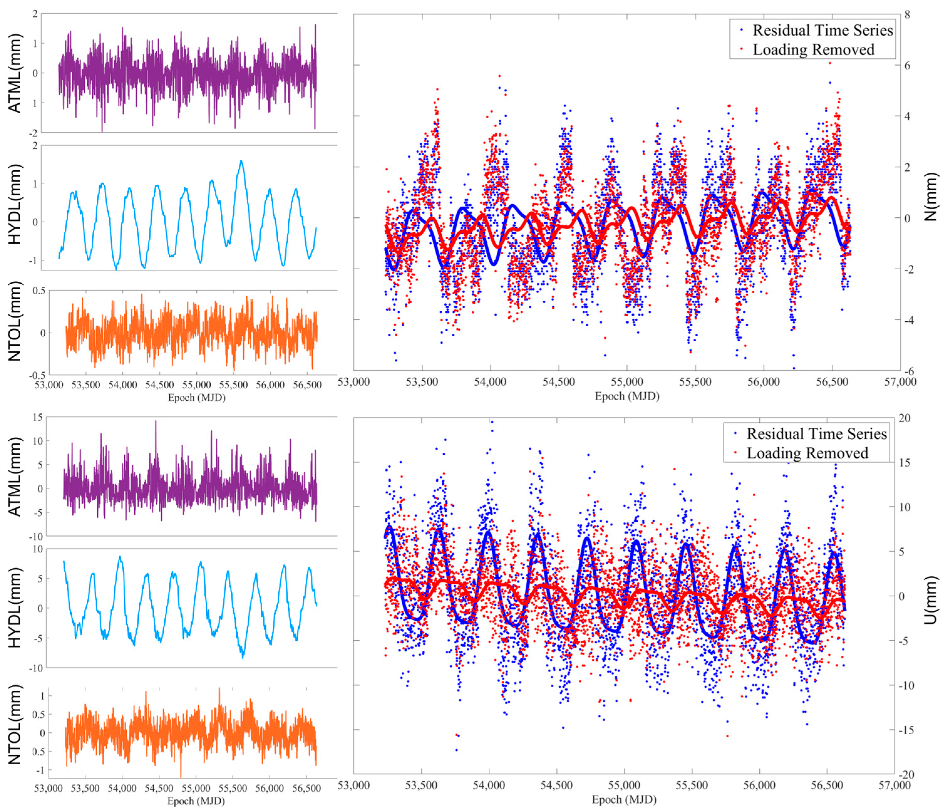
The connection between the environmental loading effects and the nonlinear motion of the reference station was analyzed in terms of periodic characteristics and correlation in this section. Figure 4 depicts the time series of ATML, HYDL, and NTOL for the three components (E, N, and U) of one station, as well as the residual time series before and after the removal of environmental loading effects. The figures reveal that ATML, HYDL, and NTOL all exhibited distinct periodic characteristics.

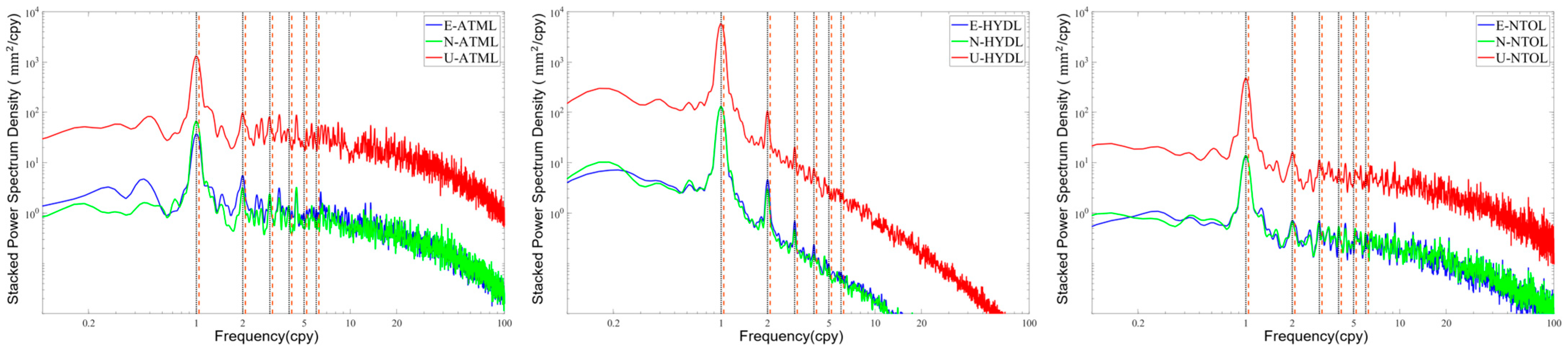
The periodicity of time series can be extracted using spectrum analysis algorithms, with the Lomb–Scargle method being one of the most commonly used methods for period extraction [32]. The Lomb–Scargle periodogram method was used to calculate the power spectrum of displacement caused by all environmental loading effects, and then the power spectrum was superimposed according to the three coordinate components of E, N, and U. Next, the results of each component were processed via Gaussian filtering to obtain the displacement stacking power spectrum caused by atmospheric loading, hydrological loading, and non-tidal ocean loading, as shown in Figure 5.

Figure 5 indicates that the displacement induced by atmospheric, hydrological, and non-tidal ocean loading exhibited similar characteristics. The most significant power spectra occurred at frequencies of 1.0 cpy and 2.0 cpy, representing annual and semi-annual signals, respectively. Additionally, the 1.04 cpy associated with the intersection-year signal and its corresponding multiple frequencies were observed, potentially due to unmodeled signal aliasing effects. On the whole, the annual and semi-annual signals remained the predominant characteristics of the environmental loading effects. Furthermore, the energy magnitude of the stacking power spectra in the E and N components was similar, whereas in the U component, it was significantly higher. This suggests that the environmental loading effects had the most obvious effect in the vertical direction for the stations, and the environmental loading effects could explain part of the periodic signal source of the GNSS coordinate time series.

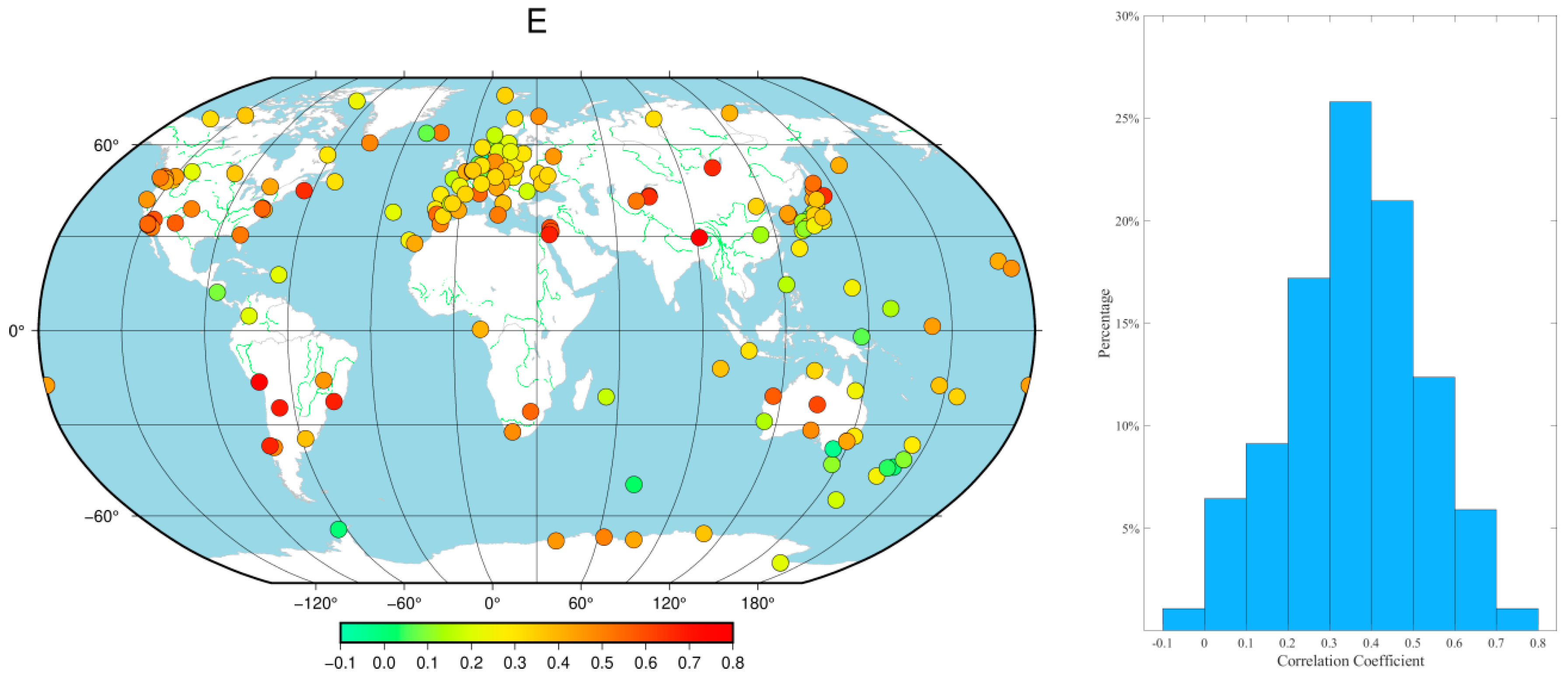
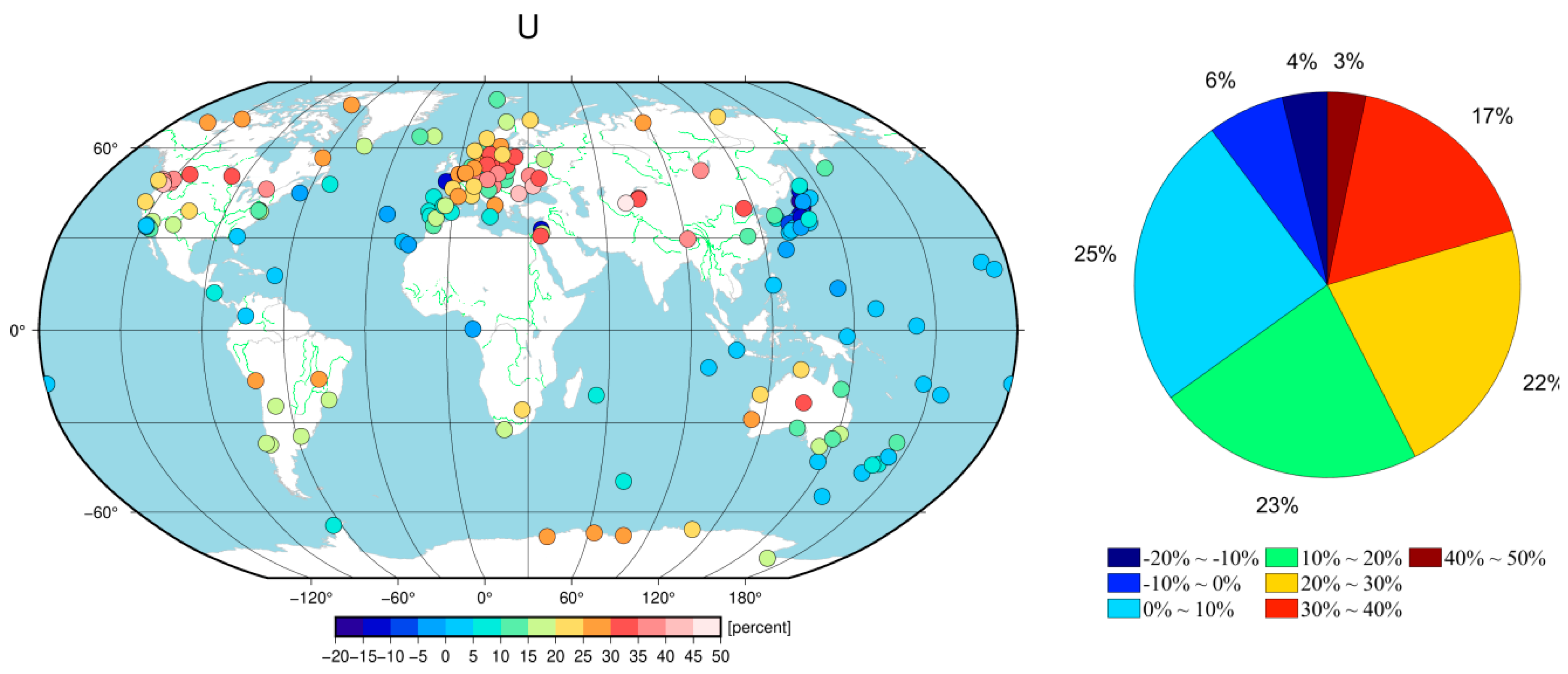
Simultaneously, the correlation between the displacement induced by the environmental loading effects and the GNSS coordinate time series was statistically analyzed. As depicted in Figure 6, the magnitude of the correlation coefficient varied with the station location. In the E direction, the majority of the stations had correlation coefficients between 0 and 0.5, accounting for approximately 79% of the total number of stations, which were mainly located in Europe and North America. A small number of stations, particularly in East Asia and parts of Europe, had correlation coefficients greater than 0.5. In the N direction, about 77% of the stations had correlation coefficients between 0 and 0.5, with a few stations exhibiting extreme negative correlation values. In the U direction, the correlation coefficients were generally higher, especially in the European region, where the proportion of stations with correlation coefficients greater than 0.5 increased significantly. The statistical results show that approximately 60% of the stations had U direction correlation coefficients greater than 0.5. Overall, the characteristics of the correlation coefficients for the E and N components were similar, yet the overall correlation was lower than that for the U component. These results highlight a significant positive correlation between environmental loading effects and GNSS time series, with environmental loading effects demonstrating stronger explanatory power in vertical nonlinear motion compared with the horizontal component.

5. Impact of Environment Loading Effects on GNSS Time Series

5.1. RMS Analysis of Residuals

To statistically evaluate the impact of atmospheric loading, hydrological loading, and non-tidal ocean loading on GNSS station nonlinear motion, ATML, HYDL and NTOL were removed from the residuals, respectively. Additionally, the percentage change in the root mean square (RMS) of GNSS time series after correction was utilized as the evaluation metric for the correction effect. A percentage value less than zero indicates an increase in the nonlinear amplitude of the stations after environmental loading effect correction, while a positive value indicates a decrease in the nonlinear amplitude:

$$RM{S}_{reduction}={\displaystyle \frac{RM{S}_{GNSS}-RM{S}_{GNSS-Loading}}{RM{S}_{GNSS}}}\times 100\%$$

(5)

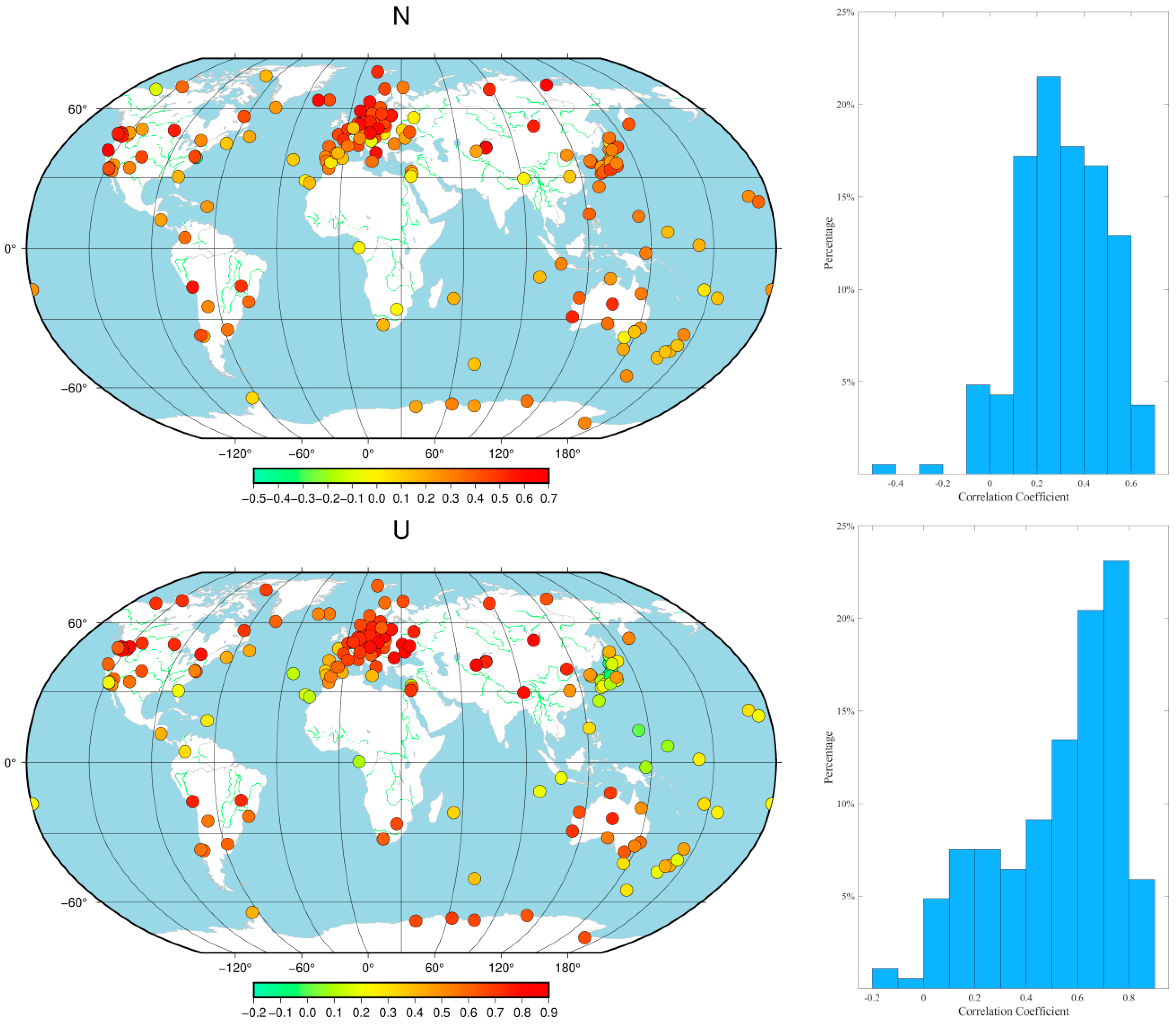
Figure 7 shows RMS percentage change pie charts of the E, N, and U components for 186 GNSS stations after removing the effects of ATML, HYDL, and NTOL environmental loads. Following the removal of the ATML, the RMS decreased in 73.1%, 83.9%, and 90.3% of the stations in the E, N, and U components of the GNSS coordinate time series, respectively, and for removal of the HYDL, the percentages were 73.7%, 63.4%, and 77.4%, respectively. Upon NTOL environmental loading effect correction, the percentages decreased to 58.1%, 62.9%, and 74.2% of the stations in the E, N, and U components, respectively.

Furthermore, the correction magnitudes of ATML and HYDL on the GNSS coordinate time series were generally higher than that of NTOL, with more significant effects. Moreover, the proportion of stations with RMS decreases greater than 10% in the U component after ATML and HYDL removal was 41.9% and 21.5%, respectively, significantly higher than those in the E and N components. In summary, the impact of environmental loading effects on the vertical direction was more pronounced than that for the horizontal direction.

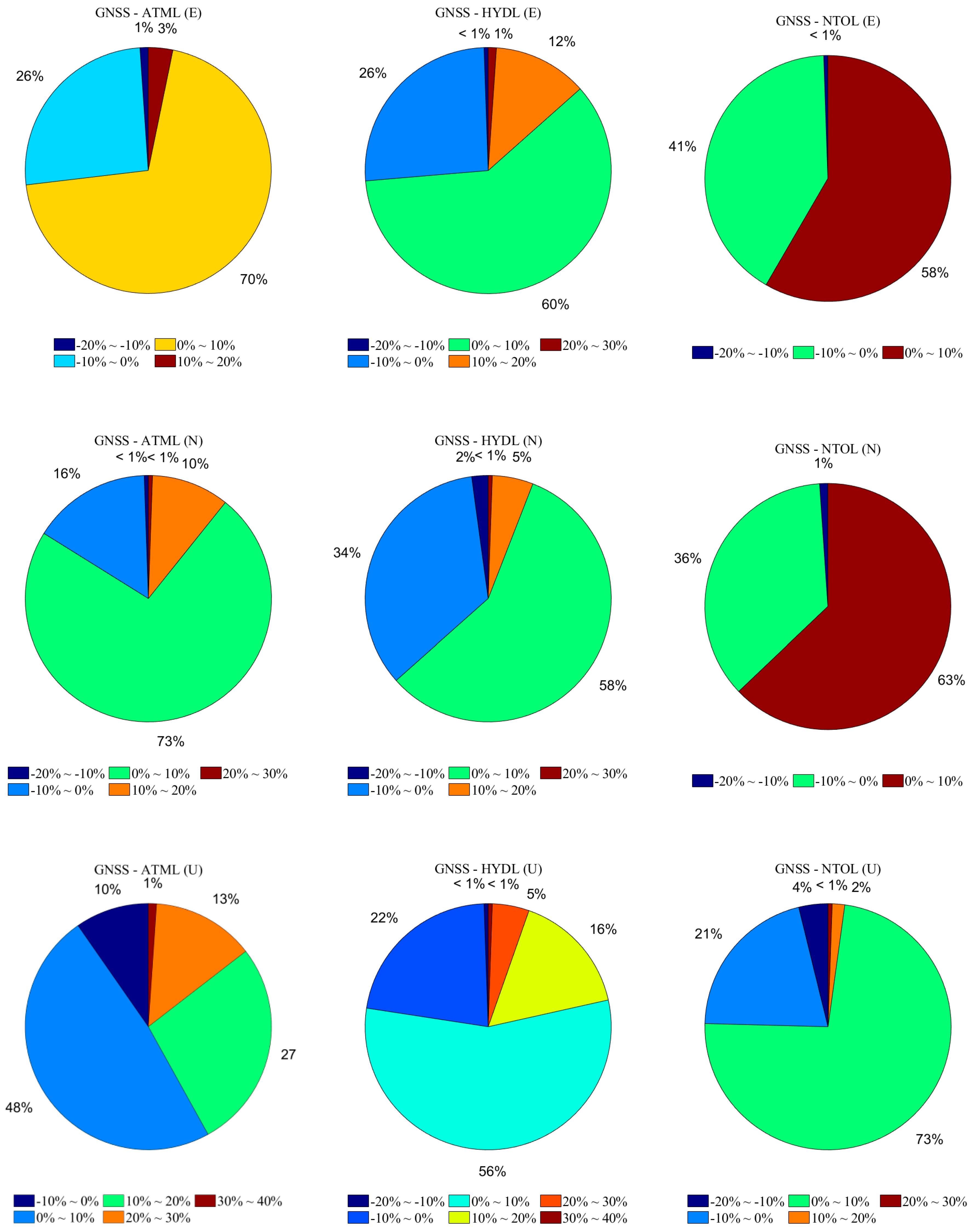
To analyze the relationship between environmental loading effects and station locations, the RMS percentage after removing the common response caused by ATML, HYDL, and NTOL from the GNSS coordinate time series was also calculated. As depicted in Figure 8, the impact of environmental loading effect correction on the coordinate time series was closely linked to the geographic location of the measurement station. Overall, 85.5%, 77.4%, and 89.8% of the stations exhibited reductions in the RMS in the E, N, and U components, respectively, with average decreases of 6.2%, 4.4%, and 16.7%, indicating that the environmental loading effects had a large contribution to the vertical nonlinear motion but a weak impact on the horizontal displacement.

However, the impact of environmental loading effects varied across different regions of stations. Correction effects near the equator tended to be smaller compared with those in middle and high latitudes, potentially due to the influence of atmospheric loading. Inland stations typically experienced more pronounced effects than coastal or marine stations. For instance, the effect of environmental loads was significant in Europe and North America, while the effect was small in Japan and the Pacific Ocean. Furthermore, disparities in water and land distribution and vegetation between the Northern and Southern Hemispheres resulted in divergent post-correction effects for the environmental loads. Generally, the Northern Hemisphere exhibited a higher RMS percentage decrease compared with the Southern Hemisphere.

5.2. Influence on Noise Properties

Geophysical effects and system errors associated with GNSS technology are generally considered potential sources of colored noise [33,34]. To investigate the impact of environmental loading effects on station noise characteristics, maximum likelihood estimation (MLE) is employed to estimate noise characteristics before and after correction [35]. Five noise types, including white noise (WN), white noise + flicker noise (WN + FN), white noise + power-law noise (WN + PL), white noise + random walk noise (WN + RWN), and white noise + flicker noise + random walk noise (WN + FN + RWN), were selected as experimental parameters.

The MLE values vary across different noise models, with the model corresponding to the maximum MLE typically selected as the optimal noise model. However, with an increase in the parameters to be estimated, the effectiveness of MLE as an evaluation index gradually diminishes. Therefore, the Akaike information criterion (AIC) and Bayesian information criterion (BIC) were used as evaluation indexes in this study. The AIC and BIC quantify the information loss of the model compared to the true model and can be expressed as follows [36]:

$$\left\{\begin{array}{l}ratio={\displaystyle \frac{AIC}{BIC}}={\displaystyle \frac{2w-2\log (L)}{\log (n)w-2\log (L)}}\\ BI{C}_{tp}=\log ({\displaystyle \frac{n}{2\pi }})w-2\log (L)\end{array}\right.$$

(6)

where $w$ is the number of parameters to be estimated and $n$ is the size of the dataset. Typically, the $ratio$ of $AIC/BIC$ is used as the criterion for judging the optimal noise model. In practice, in addition to the $ratio$, it is necessary to reintroduce a factor of 2π in the derivation to just $BIC$. This adjustment is aimed at reducing the penalty for adding more parameters in the noise model, which is referred to as $BI{C}_{tp}$. Finally, a comprehensive judgment is made according to the value of $BI{C}_{tp}$.

Table 2. Changes in optimal noise combination in residual coordinate time series before and after environmental loading effect correction.

Noise	E		N		U
	Before	After	Before	After	Before	After
WN	0	0	0	0	0	0
WN + FN	155	148	129	127	107	127
WN + FN + RWN	9	18	25	38	0	0
WN + PL	22	19	29	13	79	59
WN + RWN	0	1	3	8	0	0

presents the optimal noise combinations before and after environmental loading effect correction. The results indicate that for most stations, the optimal noise models in different components could be represented by WN + FN or WN + PL, while a few stations required combinations such as WN + RWN or WN + FN + RWN. After environmental loading effect correction, there was a slight increase in the proportion of random walk noise. However, overall, the correction of environmental loading effects did not significantly alter the optimal noise combinations for the stations.

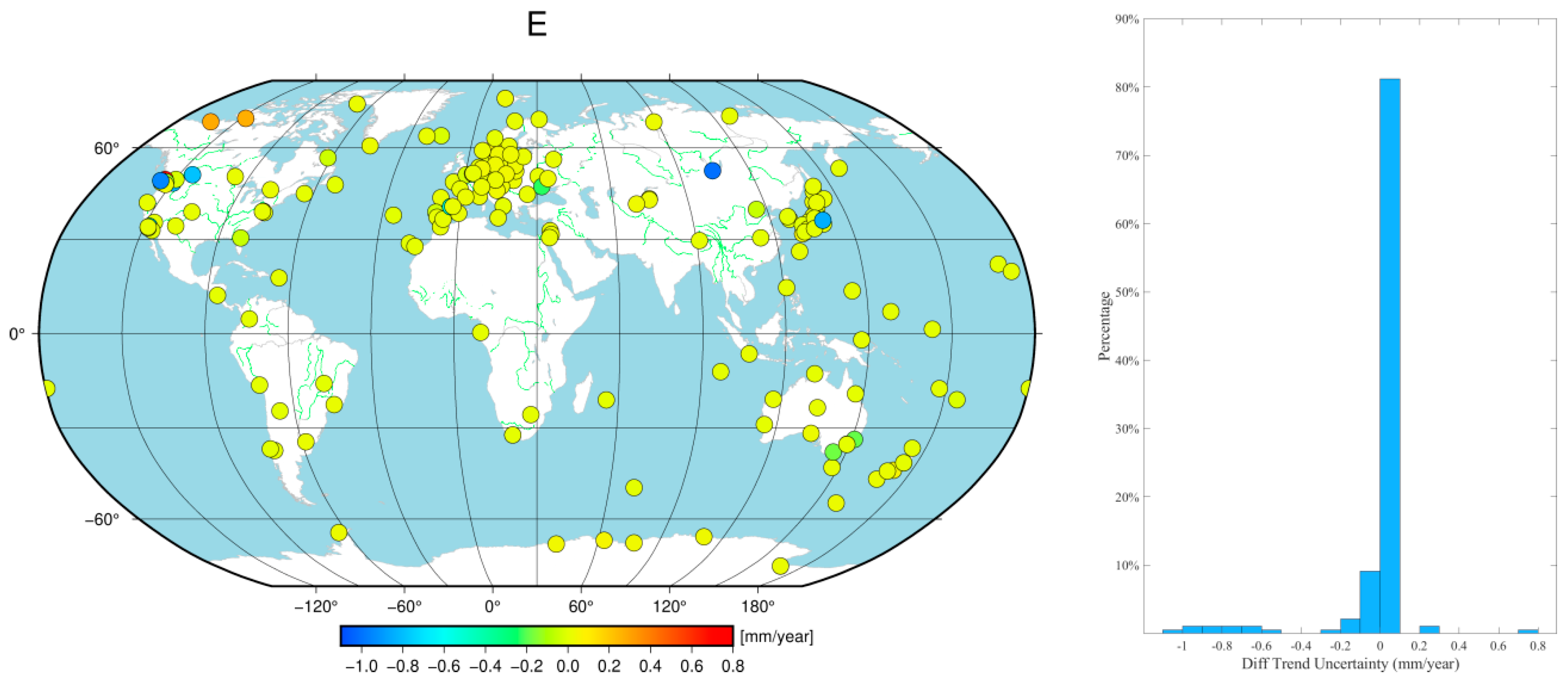
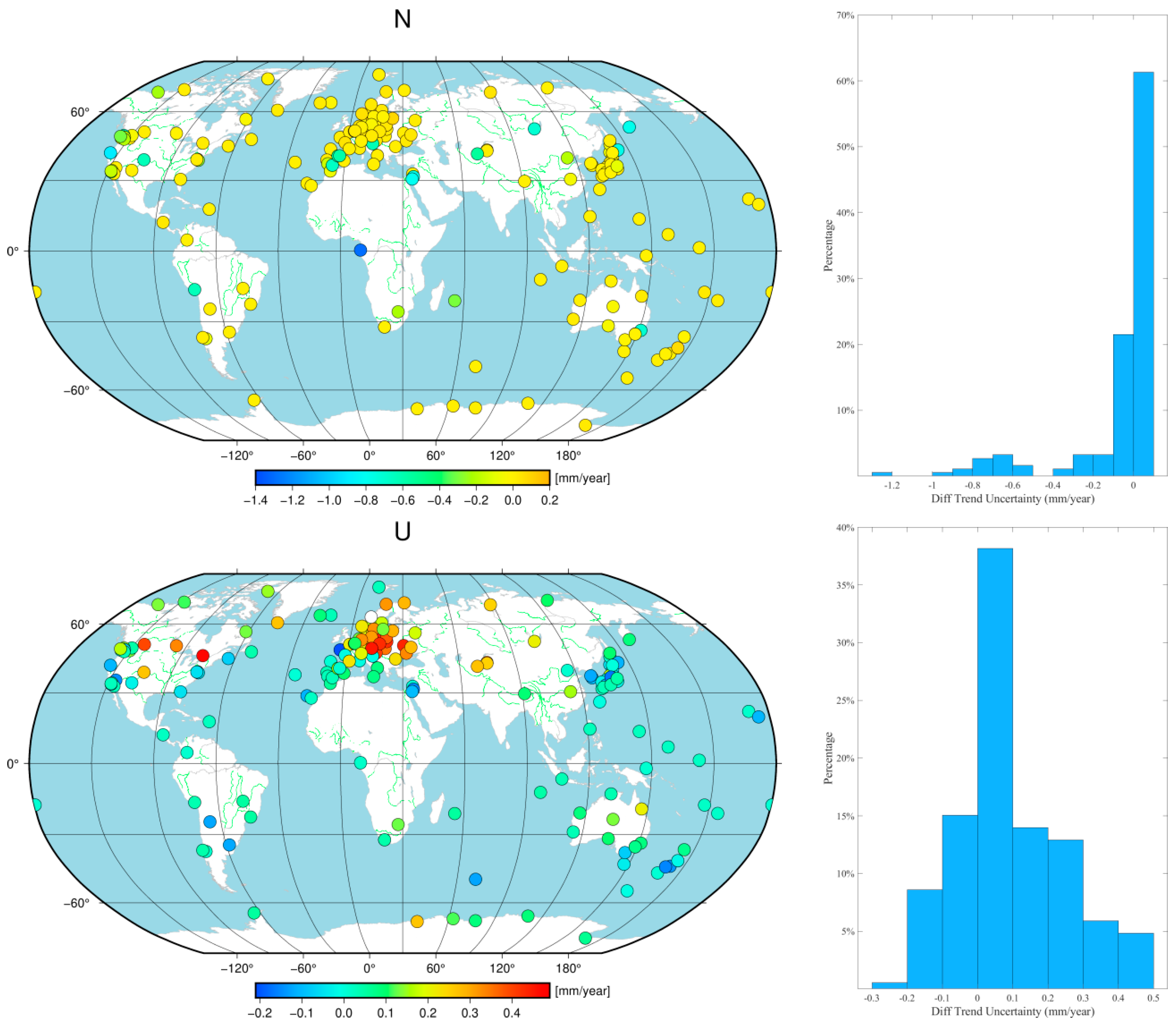
Prior research findings have indicated that the velocity uncertainty of GNSS coordinate time series varies with changes in the noise model. Therefore, this study further explored the changes in velocity uncertainty after removing environmental loading effects. The results show that the velocity uncertainties in the E and N components changed, on average, by 0.07 mm/year and 0.10 mm/year, respectively, with 90.3% and 82.8% of the stations in the E and N components experiencing changes within 0.1 mm/year, respectively. Only a few stations exhibited significant changes in velocity uncertainty, identified by blue, cyan, and orange markers in Figure 9, which had random walk noise included in their optimal noise models. It is noteworthy that the optimal noise models for the U component did not include random walk noise either before or after correction, resulting in no significant individual station changes in velocity uncertainty. The average change in velocity uncertainty in the U component was 0.13 mm/year, with 89.2% of the stations experiencing changes within 0.3 mm/year. This finding is consistent with previous research, as Langbein (2012), Dmitrieva et al. (2015), Klos et al. (2018), and He et al. (2019) found that when considering random noise models, velocity uncertainty significantly increases, as supported by the results of this study [36,37,38,39]. Furthermore, the findings revealed that 82.3%, 58.6%, and 75.8% of the stations experienced a reduction in velocity uncertainty in the E, N, and U components, respectively, following the correction of environmental loading effects. Overall, the correction of environmental loading effects had a significant impact on velocity estimation. Therefore, when establishing a millimeter-level coordinate framework, both environmental loading effect correction and consideration of optimal noise models are crucial factors to be taken into account.

5.3. Contributions to Seasonal Variations

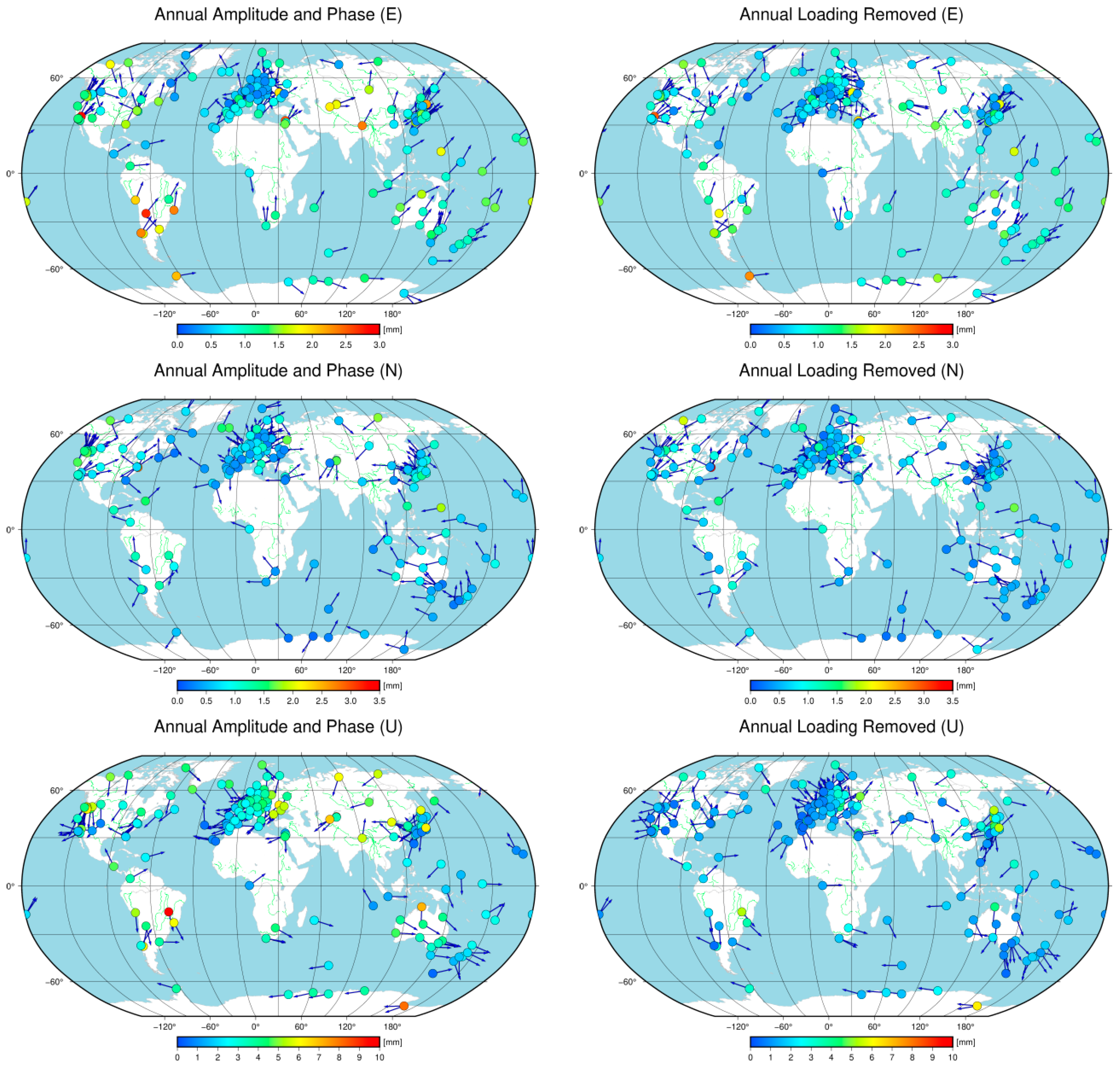
Furthermore, we conducted additional calculations to assess the annual amplitude and phase changes before and after the removal of environmental loading effects, as depicted in Figure 10. It can be observed that the annual amplitudes in the E, N, and U components for most stations decreased to varying degrees. Specifically, in the E component, the average annual amplitude decreased from 0.98 mm to 0.82 mm, representing a 16.7% decrease. In the N component, the average annual amplitude decreased from 0.76 mm to 0.66 mm, a 12.7% decrease. Notably, in the U component, the average annual amplitude significantly decreased from 3.30 mm to 1.88 mm, indicating a 43.1% decrease. The extent of the change in the station annual amplitudes appeared to be correlated with the stations’ locations, suggesting a match between the locations of environmental loads and the surrounding environments of the stations. The arrows in the figure represent the corresponding phase angles, with most stations showing no significant changes in the annual phase angles. Specifically, the average annual phase changes were 5.6 degrees, 3.1 degrees, and 11.6 degrees in the E, N, and U components, respectively.

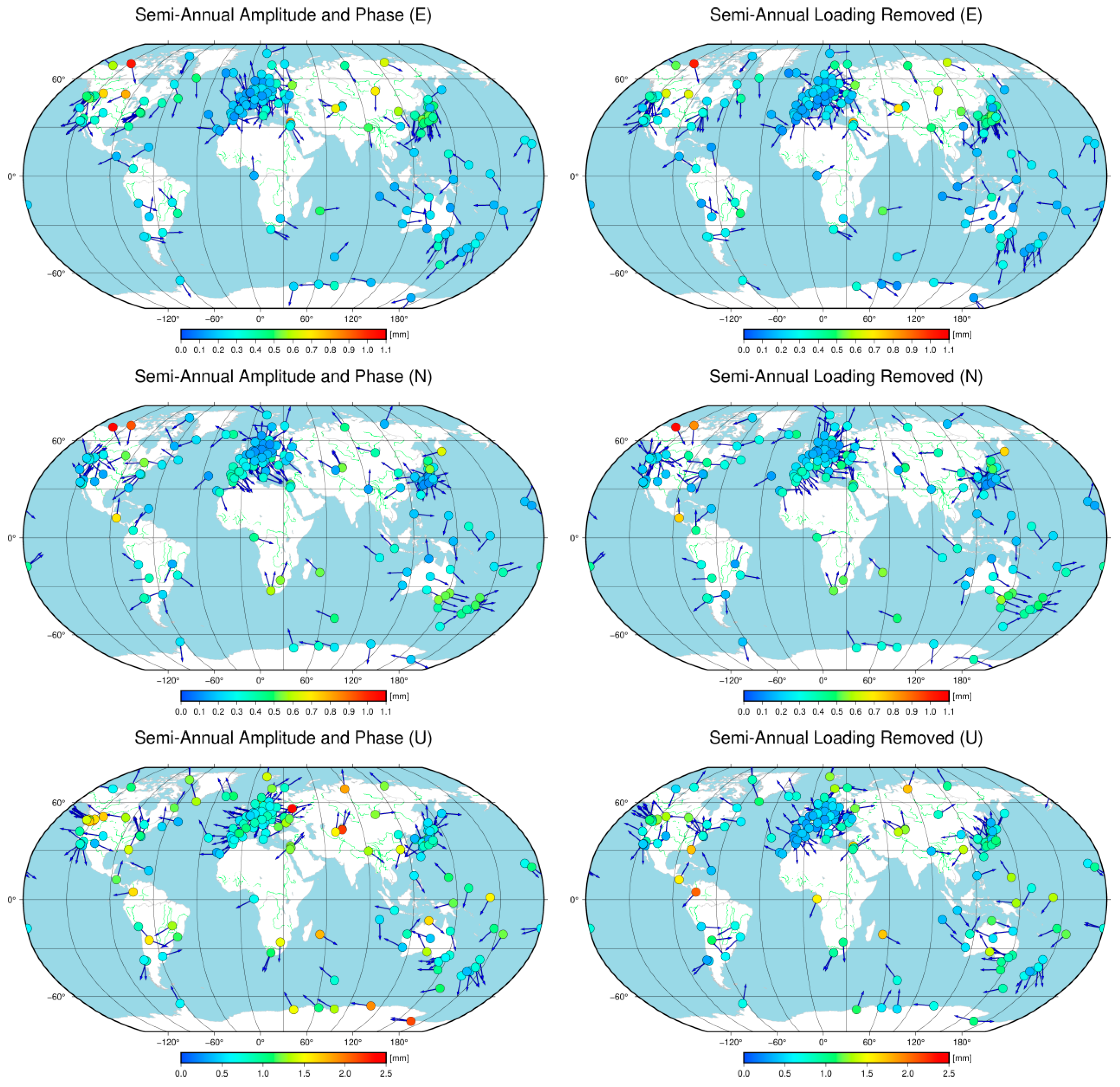
The semi-annual amplitude and phase changes exhibited similarities to the annual variations. Specifically, in the E component, there was an average decrease of 6.7%, while in the N component, there was no significant decrease observed. However, in the U component, there was an average decrease of 19.9%. The correction effect for the U component was generally greater than those for the E and N components. The changes in the semi-annual phase angles for the stations were not pronounced. The results from Figure 10 and Figure 11 can provide further insights into the reasons behind the changes in the RMS percentages depicted in Figure 8.

6. Discussion and Conclusions

The displacement of stations caused by atmospheric, hydrological, and non-tidal ocean loading was calculated in this study, and the contribution of environmental loading effects to nonlinear variation in the coordinate time series was further quantified. Additionally, the impact of environmental loading effect correction on the noise estimation and velocity estimation of GNSS coordinate time series was primarily investigated, and the following conclusions were drawn.

The magnitude of displacement induced by environmental loading effects varies, depending on the reference station’s location. The atmospheric loading primarily fluctuated within the range of ±5 mm in the U component, with fluctuations in the E and N components typically staying within ±1 mm. Station displacement was notably more pronounced in high-latitude regions compared with mid- and low-latitude areas. Hydrological loading magnitudes ranged within ±5 mm in the U component n and typically within ±0.8 mm in the E and N components, with inland areas generally experiencing greater displacements than coastal regions. Displacement resulting from non-tidal ocean loading typically fluctuated within ±0.5 mm in the E and N components, while magnitudes in the U component typically fluctuated within ±2 mm. Stations in offshore regions were impacted more than inland stations.

The environmental loads significantly influenced the vertical nonlinear motion of GNSS stations but had a limited effect on horizontal displacement. The average correlation coefficients between the displacement caused by environmental loading effects and GNSS coordinate time series in the E, N, and U components were 0.35, 0.31, and 0.52, respectively. The proportion of stations with correlation coefficients exceeding 0.5 was 19.3%, 16.7%, and 62.9%, respectively. Upon removing the impact of environmental loading effects, 85.5%, 77.4% and 89.8% of the stations experienced a decrease in RMS in the E, N, and U components, with average reduction rates of 6.2%, 4.4%, and 16.7%, respectively. Furthermore, the annual and semi-annual signals were the primary characteristic signals of environmental loading effects, and the stacking power spectrum in the U component significantly exceeded those in the E and N components.

After correction of the environmental loading effects of GNSS coordinate time series, the optimal noise model combination of measurement stations remained largely unchanged, yet it impacted the magnitude of the velocity uncertainty. Specifically, variations within 0.1 mm/year occurred for 90.3% and 82.8% of the stations in the E and N components, respectively, while 89.2% of the stations experienced variations within 0.3 mm/year in the U component. These findings offer valuable insights for establishing a millimeter-scale coordinate framework.

The environmental loads model may not be entirely consistent with the nonlinear movement of the reference station. Displacement caused by environmental loading effects can explain some of the annual and semiannual amplitudes in the vertical components. Following correction, the average decrease in the annual and semiannual amplitudes in the U component was 43.1% and 19.9%, respectively, with the average change in the annual and semiannual phases being less than 12 degrees.

References

- Jiang, W.; Li, Z.; Wei, N.; Liu, J. Progress and thoughts on establishment of geodetic coordinate frame. Acta Geod. Cartogr. Sin. 2022, 51, 1259. [Google Scholar] [CrossRef]
- Wu, S.; Li, Z.; Li, H.; Bian, S.; Ouyang, H.; Yao, Y.; Peng, P.; He, Y. Detection of Periodic Signals with Time-varying Coefficients from CMONOC Stations in China by Singular Spectrum Analysis. IEEE Trans. Geosci. Remote Sens. 2023, 61, 5802812. [Google Scholar] [CrossRef]
- Shu, B.; He, Y.; Wang, L.; Zhang, Q.; Li, X.; Qu, X.; Huang, G.; Qu, W. Real-time high-precision landslide displacement monitoring based on a GNSS CORS network. Measurement 2023, 217, 113056. [Google Scholar] [CrossRef]
- Dong, D.; Fang, P.; Bock, Y.; Cheng, M.K.; Miyazaki, S. Anatomy of apparent seasonal variations from GPS-derived site position time series. J. Geophys. Res. Solid Earth 2002, 107, ETG 9-1–ETG 9-16. [Google Scholar] [CrossRef]
- Yan, H.; Chen, W.; Zhu, Y.; Zhong, M. Contributions of thermal expansion of monuments and nearby bedrock to observed GPS height changes. Geophys. Res. Lett. 2009, 36, L13301. [Google Scholar] [CrossRef]
- Fang, M.; Dong, D.; Hager, B.H. Displacements due to surface temperature variation on a uniform elastic sphere with its centre of mass stationary. Geophys. J. Int. 2014, 196, 194–203. [Google Scholar] [CrossRef]
- Gobron, K.; Rebischung, P.; Van Camp, M.; Demoulin, A.; de Viron, Q. Influence of aperiodic non-tidal atmospheric and oceanic loading deformations on the stochastic properties of global GNSS vertical land motion time series. J. Geophys. Res. Solid Earth 2021, 126, e2021JB022370. [Google Scholar] [CrossRef]
- Li, X.; Zhong, B.; Li, J.; Wang, H. Investigating Terrestrial Water Storage Changes and Their Driving Factors in the Southwest River Basin of China Using Geodetic Data. IEEE Trans. Geosci. Remote Sens. 2023, 61, 5922115. [Google Scholar] [CrossRef]
- Lu, R.; Li, Z.; Chen, Q.; Ding, X.; Yang, K.; Zhang, M.; Lu, Y.; Fan, W.; Chen, H.; Jiang, W. On the contributions of refined thermal expansion model to nonlinear variations in different GNSS height time series products. GPS Solut. 2024, 28, 80. [Google Scholar] [CrossRef]
- Li, Z.; Chen, W.; van Dam, T.; Rebischung, P.; Altamimi, Z. Comparative analysis of different atmospheric surface pressure models and their impacts on daily ITRF2014 GNSS residual time series. J. Geod. 2020, 94, 42. [Google Scholar] [CrossRef]
- Blewitt, G.; Lavallée, D.; Clarke, P.; Nurutdinov, K. A new global mode of Earth deformation: Seasonal cycle detected. Science 2001, 294, 2342–2345. [Google Scholar] [CrossRef]
- Gegout, P.; Boy, J.P.; Hinderer, J.; Ferhat, G. Modeling and observation of loading contribution to time-variable GPS sites positions. In Proceedings of the Gravity, Geoid and Earth Observation: IAG Commission 2: Gravity Field, Chania, Greece, 23–27 June 2008; Springer: Berlin/Heidelberg, Germany, 2010; pp. 651–659. [Google Scholar] [CrossRef]
- Jiang, W.; Li, Z.; van Dam, T.; Ding, W. Comparative analysis of different environmental loading methods and their impacts on the GPS height time series. J. Geod. 2013, 87, 687–703. [Google Scholar] [CrossRef]
- van Dam, T.; Collilieux, X.; Wuite, J.; Altamimi, Z.; Ray, J. Nontidal ocean loading: Amplitudes and potential effects in GPS height time series. J. Geod. 2012, 86, 1043–1057. [Google Scholar] [CrossRef]
- Xu, X.; Dong, D.; Fang, M.; Zhou, Y.; Wei, N.; Zhou, F. Contributions of thermoelastic deformation to seasonal variations in GPS station position. GPS Solut. 2017, 21, 1265–1274. [Google Scholar] [CrossRef]
- Yuan, P.; Li, Z.; Jiang, W.; Ma, Y.; Chen, W.; Sneeuw, N. Influences of environmental loading corrections on the nonlinear variations and velocity uncertainties for the reprocessed global positioning system height time series of the crustal movement observation network of China. Remote Sens. 2018, 10, 958. [Google Scholar] [CrossRef]
- Haritonova, D. The impact of the Baltic Sea non-tidal loading on GNSS station coordinate time series: The case of Latvia. Balt. J. Mod. Comput. 2019, 7, 541–549. [Google Scholar] [CrossRef]
- Niu, Y.; Wei, N.; Li, M.; Rebischung, P.; Shi, C.; Chen, G. Quantifying discrepancies in the three-dimensional seasonal variations between IGS station positions and load models. J. Geod. 2022, 96, 31. [Google Scholar] [CrossRef]
- Bevis, M.; Alsdorf, D.; Kendrick, E.; Fortes, L.P.; Forsberg, B.; Smalley, R.; Smalley, R., Jr.; Becker, J. Seasonal fluctuations in the mass of the Amazon River system and Earth’s elastic response. Geophys. Res. Lett. 2005, 32, L16308. [Google Scholar] [CrossRef]
- Van Dam, T.; Wahr, J.; Milly, P.C.D.; Shmakin, A.B.; Blewitt, G.; Lavallee, D.; Larson, K.M. Crustal displacements due to continental water loading. Geophys. Res. Lett. 2001, 28, 651–654. [Google Scholar] [CrossRef]
- Fritsche, M.; Döll, P.; Dietrich, R. Global-scale validation of model-based load deformation of the Earth’s crust from continental watermass and atmospheric pressure variations using GPS. J. Geodyn. 2012, 59, 133–142. [Google Scholar] [CrossRef]
- Moreira, D.M.; Calmant, S.; Perosanz, F.; Xavier, L.; Rotunno Fiho, O.C.; Seyler, F.; Monterio, A.C. Comparisons of observed and modeled elastic responses to hydrological loading in the Amazon basin. Geophys. Res. Lett. 2016, 43, 9604–9610. [Google Scholar] [CrossRef]
- Zhang, J.; Li, Z.; Zhang, P.; Yang, F.; Wu, J.; Liu, X.; Wang, X.; Tan, Q. Assessing the Nonlinear Changes in Global Navigation Satellite System Vertical Time Series with Environmental Loading in Mainland China. Remote Sens. 2023, 15, 4115. [Google Scholar] [CrossRef]
- Nahmani, S.; Bock, O.; Bouin, M.N.; Santamaria, A.; Boy, J.P.; Collilieux, X.; Metivier, L. Hydrological deformation induced by the West African Monsoon: Comparison of GPS, GRACE and loading models. J. Geophys. Res. Solid Earth 2012, 117, B05409. [Google Scholar] [CrossRef]
- Wu, Q.; Pan, Y.; Ding, H.; Xiao, Y.; He, Y. Quantifying the effect of non-seasonal non-tidal loadings on background noise properties of GPS vertical displacements in mainland China. Measurement 2023, 217, 113007. [Google Scholar] [CrossRef]
- He, Y.; Nie, G.; Wu, S.; Li, H. Comparative analysis of the correction effect of different environmental loading products on global GNSS coordinate time series. Adv. Space Res. 2022, 70, 3594–3613. [Google Scholar] [CrossRef]
- Altamimi, Z.; Rebischung, P.; Métivier, L.; Collilieux, X. ITRF2014: A new release of the International Terrestrial Reference Frame modeling nonlinear station motions. J. Geophys. Res. Solid Earth 2016, 121, 6109–6131. [Google Scholar] [CrossRef]
- Farrell, W.E. Deformation of the Earth by surface loads. Rev. Geophys. 1972, 10, 761–797. [Google Scholar] [CrossRef]
- Chan, P.K.; Gao, B.C. A comparison of MODIS, NCEP, and TMI sea surface temperature datasets. IEEE Geosci. Remote Sens. Lett. 2005, 2, 270–274. [Google Scholar] [CrossRef]
- Syed, T.H.; Famiglietti, J.S.; Rodell, M.; Chen, J.; Wilson, C.R. Analysis of terrestrial water storage changes from GRACE and GLDAS. Water Resour. Res. 2008, 44, W02433. [Google Scholar] [CrossRef]
- Kim, S.B.; Lee, T.; Fukumori, I. Mechanisms controlling the interannual variation of mixed layer temperature averaged over the Niño-3 region. J. Clim. 2007, 20, 3822–3843. [Google Scholar] [CrossRef]
- VanderPlas, J.T. Understanding the lomb–scargle periodogram. Astrophys. J. Suppl. Ser. 2018, 236, 16. [Google Scholar] [CrossRef]
- Williams, S.D.P.; Bock, Y.; Fang, P.; Jamason, P.; Nikolaidis, R.M.; Prawirodirdjo, L.; Miller, M.; Johnson, D. Error analysis of continuous GPS position time series. J. Geophys. Res. 2004, 109, B03412. [Google Scholar] [CrossRef]
- Williams, S.D.P. The effect of coloured noise on the uncertainties of rates estimated from geodetic time series. J. Geod. 2003, 76, 483–494. [Google Scholar] [CrossRef]
- Bos, M.S.; Fernandes, R.M.S.; Williams, S.D.P.; Bastos, L. Fast error analysis of continuous GNSS observations with missing data. J. Geod. 2013, 87, 351–360. [Google Scholar] [CrossRef]
- He, X.; Bos, M.S.; Montillet, J.P.; Fernandes, R.M.S. Investigation of the noise properties at low frequencies in long GNSS time series. J. Geod. 2019, 93, 1271–1282. [Google Scholar] [CrossRef]
- Langbein, J. Estimating rate uncertainty with maximum likelihood: Differences between power-law and flicker–random-walk models. J. Geod. 2012, 86, 775–783. [Google Scholar] [CrossRef]
- Dmitrieva, K.; Segall, P.; DeMets, C. Network-based estimation of time-dependent noise in GPS position time series. J. Geod. 2015, 89, 591–606. [Google Scholar] [CrossRef]
- Klos, A.; Olivares, G.; Teferle, F.N.; Hunegnaw, A.; Bogusz, J. On the combined effect of periodic signals and colored noise on velocity uncertainties. GPS Solut. 2018, 22, 1. [Google Scholar] [CrossRef]
Figure 1.
Global distribution of 186 stations. Modified, Julian Day 53232–56631.
Figure 2.
The spatial distribution of the mean absolute displacements caused by environmental loading effects in the east (E), north (N), and up (U) components at 186 GNSS stations. The color scale ranges from 0.0 to 0.9 mm for the east and north components and from 0.0 to 5.1 mm for the up components.
Figure 3.
Normal distribution and probability of ATML, HYDL, and NTOL.
Figure 4.
Time series of residuals in E, N, and U components and ATML, HYDL, and NTOL time series at one station. From top to bottom, figures show representations of E, N, and U components. (left) Purple, light blue, and brown-yellow colors represent ATML, HYDL, and NTOL, respectively. (right) The blue color is the residual time series, and the red color is the time series after removing the environmental loading effects.
Figure 5.
Stacking power spectra of ATML, HYDL, and NTOL for E, N, and U at 186 GNSS stations: (left) E component, (middle) N component, and (right) U component. In the graph, the red, green, and blue curves represent the U, N, and E components, respectively, while vertical solid and dashed lines represent 1.0 (black) and 1.04 cycles per year (cpy) (red) and their integer multiples. Power spectral density unit = mm2/cpy.
Figure 6.
Correlation coefficient distribution and histogram of environmental loading effects in E, N, and U components.
Figure 7.
RMS percentage change pie charts of E, N, and U components for 186 GNSS stations after removal of ATML, HYDL, and NTOL environmental loading effects.
Figure 8.
Distribution and pie charts of RMS percentage change after removal of environmental loading effects for E, N, and U components.
Figure 9.
Distribution and bar graph of velocity uncertainty change after removing environmental loading effects in E, N, and U components.
Figure 10.
Schematic diagram of annual amplitude and phase before and after removing environmental loading effects in E, N, and U components. The legend range for the E component is 0.0–3.0 mm, the legend range for the N component is 0.0–3.5 mm, and the legend range for the U component is 0.0–10.0 mm. The arrow points to represent the phase angle.
Figure 11.
Schematic diagram illustrating the semi-annual amplitude and phase in the E, N, and U components before and after removing environmental loading effects. The legend range is 0.0–1.1 mm for the E and N components and 0.0–2.5 mm for the U component. Arrows indicate the phase angle.