Detection-Oriented Evaluation of SAR Dexterous Barrage Jamming Effectiveness

Abstract

The assessment of the jamming effect of Synthetic Aperture Radar (SAR) is the primary means to measure the reliability of the jamming, which can provide important guidance for the use of jamming strategies and patterns. This paper proposes a detection-oriented evaluation of the effect of SAR dexterous barrage jamming. Starting from the detection, it divides the evaluation process into two stages: (1) for the case in which the target can be detected under the jamming scenario, two feature parameters, namely, the target exposion area and target relative magnitude, are extracted; (2) for the case in which the target cannot be detected under the jamming scenario, another three feature parameters, namely, jamming relative magnitude, average edge brightness, and local information entropy, are extracted. On this basis, two hierarchical evaluation candidates, the target exposure degree and jamming concealment degree, respectively, are designed, and a comprehensive evaluation index of the dexterous suppression degree is finally proposed. Jamming experiments are carried out from real and simulated SAR data with different scenarios, and the results demonstrate that the proposed method effectively measures the barrage jamming effects of different jamming-to-signal ratios and patterns. More importantly, it quantifies the relationship between suppression degree and detection rate, wherein the detection rate decreases by about 35% to 45% for every 0.1 increase in the suppression degree.

1. Introduction

Synthetic Aperture Radar (SAR) has become an important reconnaissance tool in modern electronic countermeasures due to its all-weather and all-day operation, strong penetration, and high-resolution imaging advantages [1,2,3,4]. Synthetic Aperture Radar jamming refers to the active jamming of SAR through specific jamming means, so as to achieve the effect of shielding the protected target or cheating the detection radar in the SAR imaging results, which is of great significance to the protection of valuable targets against SAR reconnaissance [5]. Among them, dexterous barrage jamming is one of the widely used means that has been put into practical application. A notable event is that Russia used powerful electromagnetic jamming to cause anomalies in the Sentinel-1 satellite images, creating intense flares that effectively obscured targets and activities near the Sevastopol port [6]. Accordingly, a quantitative evaluation of the SAR dexterous barrage jamming effect can reflect the effect of SAR jamming applications and provide an important reference for the subsequent use of jamming strategies and patterns [7,8].

The assessment of the jamming effect of SAR dexterous barrage jamming can be divided into two categories: subjective and objective [9]. The subjective assessment relies on the manual interpretation of SAR images, which is limited by the knowledge and experience of the experts [10]. Therefore, current research prefers to extract quantitative indicators from the signal or image level to implement the objective assessment. For example, in terms of single-feature metrics, Ma et al. [11] propose Euclidean distance for evaluating radio frequency jamming effects. Cui et al. [12] propose an equivalent number of looks (ENL) for quantitatively evaluating frequency modulation noise jamming effects. Shi et al. [13] explore the relationship between the noise jamming power and the information entropy based on an entropy-based evaluation method. Lu et al. [14] utilize the gray-level co-occurrence matrix to evaluate the degree of mismatch in the texture features of SAR images. In terms of multi-feature indicators, Han et al. [15] modify the structural similarity index measure and propose the GSSIM index so that the evaluation results are highly consistent with human visual perception. Liu et al. [16] propose corresponding evaluation formulas for the effects of deception jamming and barrage jamming through neural networks, which realize the quantitative evaluation of different jamming effects. Liu et al. [17] combine the image texture and contour and propose an evaluation method to assess the relationship between image structure similarity and image contour matching degree. Liu et al. [18] use a Back Propagation (BP) neural network to reduce the impacts of human factors in the process of index association and improve assessment accuracy. Han et al. [19] simulate human visual characteristics through two-dimensional wavelet transformation and propose a wavelet-weighted correlation coefficient, which reflects the loss of image details with more certainty.

Although the existing methods have met some success, the following deficiencies still exist:

(1)

The evaluation processes are characterized by one-sided and independent indicators, which cannot accurately reflect the changes in the overall quality of the jamming image.

(2)

The investigated jamming patterns are simple, reflecting that a comprehensive assessment of the effectiveness of dexterous barrage jamming with different shapes, areas, and magnitudes is lacking.

(3)

The existing research is stuck at feature-level and indicator-level evaluation, which do not consider detection-level evaluation and the feedback to the subsequent jamming employment.

To this end, this paper proposes an SAR dexterous suppression jamming evaluation method from the perspective of target detection. The main novelty lies in the fact that based on the classical Constant False Alarm Rate (CFAR) detection algorithm, the evaluation process is divided into two stages: “target can be detected” and “target can not be detected”. In the first stage, two feature parameters, i.e., target exposion area and target relative magnitude, are extracted, which reflects the difference between target and jamming. In the second stage, three feature parameters, i.e., jamming relative magnitude, average edge brightness, and local information entropy, are extracted, which considers the contrast between jamming and background. On this basis, two candidates, namely target exposure degree and jamming concealment degree, are designed to, respectively, evaluate the jamming effect at different stages. Combining these two candidates, a dexterous suppression degree index is finally proposed, which comprehensively reflects and assesses the jamming effect. Experiments conducted on real and simulated SAR datasets not only verify the effectiveness of the proposed method in evaluating dexterous barrage jamming with different JSRs and patterns but also prospectively qualify the relationship between dexterous suppression degree and detection rate.

2. Dataset Generation

The jamming-free measured data used in this paper are from MiniSAR collected by Sandia Labs, Albuquerque, NM, USA. MiniSAR operates in X-band and spotlight mode, and its range and azimuth resolution is 0.1 m × 0.1 by algorithms such as bilinear interpolation [20,21]. The original image size is 1638 × 2510 pixels, and the imaging scenes include sand, cities, forests, and airports. The scene contains many artificial targets, such as vehicles, airplanes, and buildings. The details of radar operating parameters are shown in

Table 1. MiniSAR radar operating parameters.

Parameters	Descriptive
Carrier frequency	10 GHz
Signal bandwidth	200 MHz
Pulse width	10 μs
Center slanting distance	5 km
Platform speed	200 m/s

.

In our work, three typical dexterous suppression templates, circle flare, rectangle flare, and Gaussian flare, are used. The pixel intensities of rectangle and circle flare jamming are satisfied with a uniform distribution, while the Gaussian flare is a non-uniformly distributed jamming. The range of JSR is set to 20–90 dB with a sample interval of 1 dB. It can be seen from Figure 1 that when the JSR is lower than 20 dB, the jamming cannot be detected, and the purpose of covering the protected target cannot be achieved at this time, so the initial value of the JSR is set to 20 dB. In contrast, at 90 dB, the JSR is too strong to conceal, thus losing evaluation significance. JSR refers to the ratio of the jamming power to the scene power in the jamming area, and then the logarithm of this ratio is taken. The scene power refers to the echo power of the scattering points in the scene.

Given the above settings, we generated 426 jamming images for two different scenarios [22]. The protected targets in these scenarios are all vehicles, where the numbers are 13 and 9, respectively. Some of the images are shown in Figure 1. The first to third rows are jamming data from a forest background, which include a total of 213 scene data (namely dataset 1). The fourth to sixth rows are datasets from a city background, which contain a total of 213 scene data (namely dataset 2). Dataset 1 is used for the establishment of feature parameters in the proposed evaluation method, and dataset 2 is used to further verify the relationship between detection rate and suppression degree. The columns from left to right denote the jamming flares with an increased JSR interval of 10 dB. As the JSR increases, the target detection becomes more arduous while the degree of difference between the jamming and the environment gradually increases.

3. Jamming Effectiveness Evaluation

As we know, the imaging of barrage jamming determines that its effectiveness evaluation is inevitably affected by JSR [23]. As the JSR increases, the jamming itself goes from imperceptible to fully exposed. In contrast, the protected target goes from fully detectable to partially detectable to entirely undetectable.

On the one hand, for the purpose of barrage jamming application, target concealment is superior to jamming concealment, so this work divides the assessment of the SAR dexterous barrage jamming effect into two stages. The first one is the target exposure to the complete covering stage, and the second one is the jamming concealment to the jamming exposure stage after the target is completely covered. On the other hand, when the protected target is entirely undetectable, the assessment of barrage jamming should be a measurement of jamming concealment, i.e., in what cases (various JSRs and patterns) the jamming cannot be detected as much as possible. When the protected target is undetectable, the assessment of barrage jamming should measure which cases (various JSRs and patterns) allow us to achieve the desired detection rate. Therefore, the entire assessment of the effectiveness of dexterous barrage jamming can be divided into two stages, i.e., the target-detectable stage and the target-undetectable stage [24].

3.1. Jamming Assessment in the Target-Detectable Stage

Currently, the standard target detection method is the CFAR algorithm, which centers on adaptively setting a detection threshold based on the statistical properties of the local background. Signals below this threshold are considered background noise, while those above it are considered targets. By analyzing the principle of CFAR, the degree of “flooding” of the target signal can be quantitatively evaluated to assess the jamming effect [25,26].

At the target detection stage, there is inevitably a brightness difference between the protected target and the surrounding environment. Therefore, we adopt the sliding window processing to filter the jamming area. The size of the sliding window is set to the target size, the area below the average brightness is excluded [27], and then, after a series of operations such as morphological filtering, the changes in the remaining area can reflect the degree of target exposure.

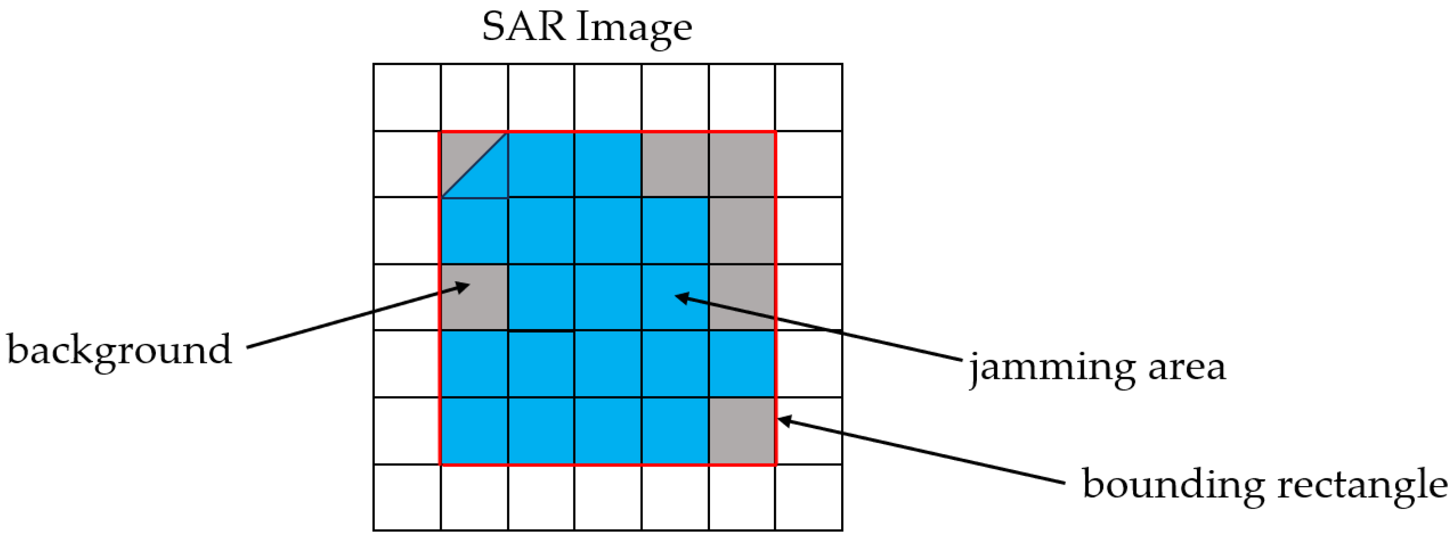
3.1.1. Target Exposion Area

For barrage jamming, if the JSR is low, the protected target will not be completely obscured [28], and at this time, a part of the target structure will be exposed. In order to quantitatively analyze the exposure degree of the protected target, we extract a target exposion area feature parameter for evaluation, which is given as

$$P_1={\displaystyle \frac{S_1}{S_2+C}}$$

(1)

Specifically, $S_1$ is the sum of the number of detected pixels of the protected object, and $S_2$ is the total number of pixels of the protected object. $C$ is a normalization factor.

According to the above formula, the target exposion area is positively correlated with the detected target area. Specifically, when $S_1$ reaches its maximum value, the target exposion area is close to 1, indicating that the jamming effect is the worst, and the target’s exposed degree reaches its highest. When no target area is detected, the value of $S_1$ will be zero, indicating that the jamming effect is optimal, and the target is completely covered. Thus, by introducing the feature parameter, the effect of jamming can be evaluated from the target area perspective.

3.1.2. Target Relative Magnitude

Similarly, the protected target being detectable indicates that the jamming failed to fuse with the protected target and there must be a brightness difference between the target and its surroundings. Therefore, a target relative magnitude feature parameter is extracted. Since the brightness difference between the target and its surroundings is in the range of [0, 255], in order to avoid the influence of the results due to the significant luminance difference, the results of the luminance difference need to be normalized, which is given as

$$P_2=1-{\displaystyle \frac{C}{|m_1-m_2|+C}}$$

(2)

Specifically, $m_1$ is the ratio of the sum of the detected pixel values to the number of detected pixel points of the protected target, and $m_2$ is the ratio of the sum of pixel values in the jamming area to the number of its pixel points. $C$ is a normalization factor. The jamming area is shown in Figure 2, which shows the non-target exposed area (gray area) within the external moments (the area wrapped by the red rectangle) of the exposed area of the detected target (blue area).

$P_2$ is positively correlated with $|m_1-m_2|$. When the average brightness of the target is close to the average brightness of the surroundings, $P_2$ approaches zero, indicating that the jamming effect is optimal at this time, and the fusion degree of the jamming area and the target area is relatively high. On the contrary, when the average brightness difference between the target area and the background increases, $P_2$ will approach 1, and the jamming effect is poor, with the lowest fusion degree of jamming area and target area. Thus, by introducing the feature parameter, the effect of jamming can be evaluated from the target brightness perspective.

3.2. Jamming Assessment in the Target-Undetectable Stage

After realizing the complete covering of the protected target, the purpose of releasing barrage jamming to protect the target is achieved [29]. However, if the jamming signal is too strong, in this case, it fails to hide its position, and instead, it will expose the protected target, As a result, in the target-undetectable stage, this section evaluates the jamming effect from the perspective of jamming concealment. Comparing the difference between jamming and the surrounding environment, the following conclusions can be drawn:

First, the histogram distribution of the jamming-free image approximates a Gaussian distribution, whereas after the jamming is applied, the histogram distribution significantly shifts to the high gray level area, reflecting that the brightness of the jamming image is significantly increased.

Second, since the jamming intensity is higher than that of the surroundings, there is an obvious transition between the edges of the jamming and the surroundings. However, there are differences in the transition degree between the surroundings and jamming with different JSRs and shapes.

Third, the higher the proximity between the jamming and surroundings, the higher the degree of jamming fusion.

Based on the above conclusions, this section extracted three feature parameters, namely, jamming relative magnitude, target edge brightness, and local information entropy, to evaluate the jamming effect.

3.2.1. Jamming Relative Magnitude

After applying dexterous barrage jamming, the histogram distribution is significantly shifted to the high gray level area and the brightness of the jamming area is enhanced [30]. Therefore, a jamming relative magnitude feature parameter is extracted to evaluate the jamming effect from the perspective of the brightness difference between the jamming and background, which is given as

$$P_3=1-{\displaystyle \frac{C}{|n_1-n_2|+C}}$$

(3)

Specifically, $n_1$ is the ratio of the sum of the pixel values in the jamming area to the number of pixel points in the jamming area. $n_2$ is the ratio of the sum of the pixel values in the background to the number of pixel points in it.

Since the JSR is relatively large in the target-undetectable stage, the jamming area is quite obvious. By setting a certain threshold, the jamming area can be segmented by using the classical bright pixel thresholding method, and the extracted jamming area is generally irregular. As shown in Figure 3, the background refers to the non-jamming area (the gray area) within the bounding rectangle (area enclosed by the red rectangle) of the jamming area (blue area).

$P_3$ is positively correlated with $|n_1-n_2|$. When the average brightness of the jamming area is close to that of the background, $P_3$ approaches zero. On the contrary, when the average brightness difference between the jamming area and the background is large, $P_3$ tends to be 1. The larger $P_3$ is, the lower the fusion degree between the jamming and surrounding, and the worse the jamming effect is. The closer $P_3$ is to 0, the better the jamming effect is. Thus, by introducing the feature parameter, the effect of jamming can be evaluated from the jamming brightness perspective.

3.2.2. Average Edge Brightness

From the above, it can be seen that there is a transition between the jamming edges and the surroundings, and there are differences in the transition degree for different jamming patterns and intensities. Therefore, the average edge brightness feature parameter is extracted to evaluate the jamming effect. The jamming edges are extracted using edge detection the classical Sobel Edge Detector [31], and the jamming effect is evaluated by comparing the extracted edge brightness, which is given as

$$P_4=1-{\displaystyle \frac{C}{e+C}}$$

(4)

Specifically, $e$ is the sharpness of the boundary between the jamming area and the background, and $C$ is the normalization factor.

In our work, the Sobel operator is employed to extract the edges of the jamming area, as shown in Figure 4; the yellow lines represent the edges of the jamming area. The ratio of the total pixel value at the jamming edges to the number of pixels is calculated, thereby obtaining the average edge brightness $e$.

When $e$ = 0, it means that the jamming area fully integrates with the background, and the concealment degree of jamming reaches its best. In this case, the boundary between the target and the background is blurred, which makes it difficult to recognize the existence of jamming. When the value of $e$ increases, it indicates that the boundary between the jamming area and the background is more apparent, which leads to an increase in the separation between the background and jamming. In this case, the jamming is easier to identify. Thus, by introducing the feature parameter, the effect of jamming can be evaluated from the degree of edge fusion between the jamming area and the background.

3.2.3. Local Information Entropy

The higher the similarity between the jamming template and the surroundings, the higher the fusion degree of jamming. Therefore, the jamming concealment degree can be quantified by evaluating the complexity of the jamming template. Thus, a local information entropy feature parameter is extracted.

The information entropy reflects the average uncertainty of the information. Favorable jamming concealment requires that the jamming template should be close to the surroundings as much as possible. Therefore, the pixel values of the jamming area, which approximate the background, are selected to calculate the local information entropy [32,33]. This focuses on the pixel similarity between the jamming area and the background so that the feature parameter can reflect the jamming concealment. The local information entropy is calculated as

$$P_5=1-{\displaystyle \frac{C}{-{\displaystyle \sum _{B}p(x_i)}{\log }_{2}p(x_i)+C}}$$

(5)

Specifically, $B$ denotes the pixel assembly selected by screening the jamming from the background. $p(x)$ represents the appearance probability of the corresponding pixel while $C$ is a normalization factor.

We set the range of $B$ to $\left[n_2-k,n_2+k\right]$. In this paper, $k$ = 50, meaning that a range of 50 pixels on the left and right of the average brightness of the background ($n_2$) is used to calculate the image entropy of the jamming area.

If $P_5$ is large, this indicates that the complexity of the jamming template is high with respect to the background. It is difficult to distinguish the jamming from the background, indicating a strong jamming concealment. Conversely, if $P_5$ is small, it means that the jamming template is relatively simple compared to the background. In this case, the jamming can be easily identified and detected, indicating weak jamming concealment. Thus, by introducing the feature parameter, the effect of jamming can be evaluated from the complexity of the template.

3.2.4. Determination of Normalization Constants

It is worth noting that the above five equations all contain the adjustment factor C, and they can be expressed in the form of Equation (6). The value of C can be determined by adopting the idea of nonlinear weighting, and it can be expressed in a generalized form as follows.

$$Y=1-{\displaystyle \frac{C}{X+C}}$$

(6)

Specifically, $X$ is the initial value of each feature parameter, $Y$ is the normalized result, and $C$ is the adjustment factor.

As is well-known, the larger the function slope, the faster the rate of dependent variable change. And the larger of function slope, the larger the value of the derivative $dY$ for $Y$. Therefore, to make the dependent variable change the fastest, the value of the derivative should be larger. Therefore, in order to make the normalized result distinguishable, it is necessary to choose the most suitable $C$, such that the sum of $dY$ and the values within the range of $X$ are maximized.

Assume that the range of $X$ is $(X_1,X_2)$, then the range of $Y$ can be set as $(Y_1,Y_2)$. The specific formula is shown in Equation (7).

$$\begin{array}{l}{S}_Y(c)={\displaystyle {\int }_{x_1}^{x_2}\frac{C}{{(X+C)}^2}}dx\\ ={\displaystyle \frac{C(x_2-x_1)}{(x_2+C)(x_1+C)}}={\displaystyle \frac{C(x_2-x_1)}{C^2+C(x_2+x_1)+x_2{x}_1}}\end{array}$$

(7)

Specifically, $S_Y(c)$ represents the change value of $dY$ within the range of $X$.

It can be observed that when $C=2\sqrt{x_1{x}_2}$, $S_Y$ reaches the maximum value. Therefore, the value of C is set as $2\sqrt{x_1{x}_2}$, where $x_1,x_2$ are the maximum and minimum values, respectively, within the variation range of each feature parameter.

The above processing is carried out to make the suppression degree more differentiated. Additionally, it aims to prevent errors from occurring in the weighted results, which might otherwise be caused by the varying ranges of feature parameters.

3.3. Two-Stage Integrated Assessment

In Section 3.2 and Section 3.3, five metrics are extracted in the target-detectable and target-undetectable stages to quantify the target exposure and jamming concealment, namely, relative exposure area, target relative magnitude, jamming relative magnitude, average edge brightness, and local information entropy. It should be noted that since the feature parameters quantify the jamming effect from different perspectives, there is no dependency among them, so the jamming effect can be comprehensively evaluated by linear operation. However, after the indicators have been normalized, the multiplication may lead to the results exceeding the expected range (e.g., the product tends to zero), making the final evaluation results not easy to interpret. Therefore, a nonlinear weighted summation strategy was further used to synthesize the feature parameters to propose a final dexterous suppression degree criterion:

$$\begin{array}{l}P=P_{TE}+P_{JC}\\ ={\displaystyle \frac{\delta }{4}}[(1-P_1)+(1-P_2)]+(1-\delta )\{0.5+{\displaystyle \frac{1}{6}}[(1-P_3)+(1-P_4)+P_5)]\}\end{array}$$

(8)

Specifically, $P$ is composed of the target exposure degree ($P_{TE}$) and jamming concealment degree ($P_{JC}$), in which the target exposure degree relates to the target exposion area and target relative magnitude, and the jamming concealment degree corresponds to the jamming relative magnitude, average edge brightness, and local information entropy.

Table 2. The range of changes in feature parameters.

	Target Exposure Degree (${\mathit{P}}_{\mathit{T}\mathit{E}}$)	Jamming Concealment Degree (${\mathit{P}}_{\mathit{J}\mathit{C}}$)
target exposion area ($P_1$)	[0.0, 1.0]	—
target relative magnitude ($P_2$)	[0.4, 1.0]	—
jamming relative magnitude ($P_3$)	—	[0.1, 0.5]
average edge brightness ($P_4$)	—	[0.2, 0.4]
local information entropy ($P_5$)	—	[0.0, 1.0]

gives the change range of the different feature parameters of 426 images in the adopted dataset. From Equation (8), it can be seen that the feature parameters and the target exposure degree are negatively correlated. The smaller the target relative magnitude and exposure area, the higher the suppression degree. Moreover, the change range of $P_{TE}$ and $P_{JC}$ with the variation of feature parameters $P_1$–$P_5$ and the change range of the target exposure degree with the variation of target relative exposure area are larger than those with the variation of target relative magnitude, which means that the target exposure degree has a more significant impact on the target exposure degree. From Equation (8), it can be seen that two feature parameters (jamming relative magnitude and average edge brightness) and jamming concealment are negatively correlated, while the local information entropy is positively correlated with jamming concealment. In addition, the change range of jamming concealment degree is the largest, second largest, and smallest with respect to the variation of local information entropy, jamming relative magnitude, and average edge brightness, respectively.

4. Analysis of Experimental Results

To verify the effectiveness and reliability of the proposed method, the forest background dataset is first used, which contains 213 jamming images with different JSRs and templates.

4.1. Feature Parameters in Target-Detectable Stage

In the target-detectable stage, the relative exposure area and target relative magnitude are used for evaluation. Part of the results are shown in Figure 5: from top to bottom, the first row to the third row show circular, rectangular, and Gaussian barrage jamming. The first to third columns denote the target relative exposure area with an increased JSR interval of 10 dB, where the white spot represents the extracted target area and the red box indicates the actual target location. The starting JSR of the leftmost image in Figure 5 is 20 dB. The fourth to sixth columns denote the target relative magnitude with an increased JSR interval of 10 dB, where the gray background outlines the central jamming area and the target relative magnitude is calculated as the intensity corresponding to the relative exposure area. Notice that the central jamming areas are all outlined by rectangles for ease of implementation.

4.2. Feature Parameters in Target-Undetectable Stage

Figure 6 gives the magnitudes of the three feature parameters in the target-undetectable stage, where (a–c) are circular, rectangular, and Gaussian jamming. The first to third columns represent the jamming relative magnitude, average edge brightness, and local information entropy. The JSRs of different jamming patterns are set to 50, 60, and 70 dB, respectively, from top to bottom. The closer the color is to red, the greater the value, and the closer the color is to blue, the smaller the value.

It can be seen that under the same jamming patterns, with the increase in JSR, the jamming relative magnitude and the average edge brightness increase, whereas the local information entropy decreases. This shows that the jamming relative magnitude and the average edge brightness are negatively correlated with the jamming concealment, while the local information entropy is positively correlated with the jamming concealment, which is in line with the expectations of the feature parameters in the target-undetectable stage. Compared with different suppression templates under the same JSR, it is found that although the jamming relative magnitude of Gaussian jamming is not much different from that of circular and rectangular jamming, the local information entropy corresponding to Gaussian jamming is much larger than that corresponding to circular and rectangular templates, indicating that Gaussian jamming is naturally integrated with the surrounding environment and has the best masking effect.

4.3. Detection-Oriented Jamming Evaluation

Combining the analysis of feature parameters in different stages, the relationship between suppression degree and JSR under different jamming patterns is plotted in Figure 7a, where the green, red, and blue curves represent the circular, rectangular, and Gaussian flare jamming patterns, respectively. In the target-detectable stage (the JSR is less than about 40 dB), the suppression degree rises on the whole as the JSR increases. The blue curves are mostly located below the red and green curves, indicating that the Gaussian flare jamming is less effective than the circular and rectangular jamming. This is attributed to the low intensity at the edge of Gaussian flare jamming with low JSRs. In addition, some targets are also located at the edge, such that the protection effect is impaired.

In the target-undetectable stage (the JSR is greater than about 40 dB), the suppression degree increases rapidly to about 0.9, followed by a decreasing trend as the JSR continues to increase. Note that the target cannot be detected when the JSR reaches a certain level, and the Gaussian flare jamming outperforms the other patterns in this stage. Figure 7b–d shows the change curves of the detection rate and suppression degree under different JSRs, where the blue curve indicates the detection rate, while the dashed curve indicates the suppression degree. The detection rate refers to the ratio of the number of detected protected targets to the total number of targets with the CFAR method. According to [34], it can be observed that the common setting range of the false alarm rate is from ${10}^{-5}$ to ${10}^{-2}$. Therefore, in our work, the constant false alarm rate is set to ${10}^{-3}$, and at this time, the protected targets in the original image can be completely detected. It can be seen that with the increase in JSR, the detection rate shows a decreasing trend and the suppression degree shows an increasing trend. The Gaussian flare jamming is clearly the least effective at target covering, as explained above.

Figure 8a,b demonstrate the linear and nonlinear fitting results between the suppression degree and detection rate for dataset 1. Since the detection rate decreases to 0 when the suppression degree is greater than 0.5, the portion of the suppression degree greater than 0.6 is not shown for a better inspection. The slopes of linear fittings for the three jamming patterns are −4.2, −3.9, and −3.9, respectively. This indicates that for every 0.1 increase in suppression degree, the detection rate decreases by about 35–45%. Meanwhile, in the nonlinear fitting results, it can be quantitatively observed that when the suppression degree is smaller than 0.3, the detection rate is greater than 0.8, while the detection rate is less than 0.4 when the suppression degree is larger than 0.4.

For a comprehensive demonstration of the evaluation, dataset 2 is further used for analysis, where the quantitative relationship between suppression degree and detection rate is presented in Figure 8c,d. In a similar manner, it can be found that the slopes of linear fittings are −4.1, −4.1, and −4.2, respectively, which verifies a consistent decrease in detection rate of about 35–45% for each 0.1 increase in suppression degree. In addition, there also exist evaluation differences between the forest and urban backgrounds. In the urban background, when the JSR is relatively low, the targets are not considerably protected (the detection rate is high) by circular, rectangular, or Gaussian flare jamming. However, with the increase in suppression degree, the jamming effect is rapidly enhanced, especially for the Gaussian flare jamming. Despite these, the observation still stands that the detection rate is greater than 0.8 when the suppression degree is smaller than 0.3, and the detection rate is less than 0.4 when the suppression degree is larger than 0.4. This verifies the effectiveness of the proposed evaluation method.

5. Discussion

In order to investigate the influence of different feature parameters on the evaluation of the jamming effect, this section discusses the variation trend of each feature parameter with the change in JSR. Figure 9 shows the relationship between different JSRs and feature parameters in the target-detectable stage with certain jamming templates. It can be observed that for the same jamming template, with the increase in JSRs, the target exposion area tends to decrease. The target relative magnitude changes little in low JSRs and increases rapidly in high JSRs. The target relative magnitude increases slowly in the early period and rapidly in the later period because more target areas are detected under low JSR conditions, resulting in insignificant differences between the target and the surrounding environment. However, under high JSR conditions, most of the target area is covered, and the brightness difference between the uncovered part and the jamming area increases, resulting in an increase in the target relative magnitude and the exposure degree of the target. Therefore, with the increase in JSR, the target exposion area will gradually increase, making the target gradually concealed. However, when the JSR increases to a certain extent, the target relative magnitude will increase rapidly. Thus, from the perspective of brightness, the exposure possibility of targets will also increase. This can be seen in Figure 10g–i. As the JSR continues to increase and the target’s exposed area further decreases, the average brightness of the target’s exposed area gradually increases.

Therefore, when selecting the optimal jamming effect, the two feature parameters should be comprehensively considered to minimize the sum of the target exposion area and target relative magnitude.

Figure 11 shows the relationship between different JSRs and jamming relative magnitude, average edge brightness, and local information entropy under circular, rectangular, and Gaussian jamming. For the same jamming template, with the increase in JSRs, the jamming relative magnitude and average edge brightness are negatively correlated with the jamming concealment degree, while the local information entropy is the opposite. In the target-undetectable stage, even if the JSR is the smallest, the three feature parameters are non-zero, such that some jamming area must be exposed when the target is completely concealed. It can also be found that when JSR reaches a certain degree, the average edge brightness tends to be stable with further increases in JSR. Notice that when the JSR is large, it is meaningless to increase the jamming concealment by adjusting the edge of the jamming area. Moreover, the variation ranges of local information entropy, jamming relative magnitude, and average edge brightness are 0.8, 0.3, and 0.2, respectively. Thus, the local information entropy has the greatest influence on jamming concealment while the average edge brightness has the least influence. Therefore, the best way to choose to increase the jamming concealment is to choose the appropriate jamming template, so that the jamming area and the surrounding environment can be integrated to the highest degree.

In summary, this paper studies the CFAR detection effect through the scattering difference between target and jamming and jamming and surrounding environment in terms of the characteristics of area, brightness, edge, shape, etc. By deriving a dexterous suppression degree, one can not only evaluate the jamming effect but also obtain feedback on the target detection rate. However, if there are only a few protected targets, the change in detection rate will be intense. As a result, it is necessary to consider more protected targets to generalize the relationship between the jamming degree and detection rate.

6. Conclusions

SAR jamming evaluation plays a crucial role in assessing the effectiveness of jamming and guiding subsequent jamming employment. However, current evaluation methods face several challenges, including the inadequate extraction of feature indicators, the insufficient investigation of jamming types, and the limited assessment of evaluation criteria. This paper proposes a detection-oriented evaluation of the effectiveness of SAR dexterous barrage jamming. First, according to whether the target is detected or not, five feature parameters, namely, target exposion area, target relative magnitude, jamming relative magnitude, average edge brightness, and local information entropy are extracted, which reflect the difference between the target and jamming as well as jamming and the background. Second, on the basis of the above feature parameters, two hierarchical evaluation candidates, i.e., target exposure degree and jamming concealment degree, respectively, are designed, which assess the abilities of target covering and the self-concealment of jamming. Third, combining these two candidates, a dexterous suppression degree is proposed to comprehensively reflect and evaluate the dexterous barrage jamming effect under different JSR and jamming patterns. Experimental results show that the proposed method not only overcomes the aforementioned limitations but also reliably evaluates the jamming effect of dexterous barrage jamming and quantifies the relationship between dexterous suppression degree and detection rate, which provides guidance for the subsequent application of jamming strategies and patterns.

References

1. Chen, T.X. Research on Synthetic Aperture Radar Jamming Effect Evaluation Method. Master’s Thesis, Strategic Support Force Information Engineering University, Zhengzhou, China, 2023. [Google Scholar]
2. Sui, R.; Wang, J.; Sun, G.; Xu, Z.; Feng, D. A Dual-Polarimetric High Range Resolution Profile Modulation Method Based on Time-Modulated APCM. IEEE Trans. Antennas Propag. 2025, 73, 1007–1017. [Google Scholar] [CrossRef]
3. Quan, S.; Zhang, T.; Xing, S.; Wang, X.; Yu, Q. Maritime ship detection with concise polarimetric characterization pattern. Int. J. Appl. Earth Obs. Geoinf. 2024, 131, 103954. [Google Scholar] [CrossRef]
4. Wang, J.; Quan, S.; Xing, S.; Li, Y.; Wu, H.; Meng, W. PSO-Based fine polarimetric decomposition for ship scattering characterization. ISPRS J. Photogramm. Remote Sens. 2025, 220, 18–31. [Google Scholar] [CrossRef]
5. Yang, Y. Research on the Evaluation Method of SAR Jamming Effect Based on Autoencoder. Master’s Thesis, Xidian University, Xi’an, China, 2022. [Google Scholar]
6. Han, G.Q.; Wu, X.F.; Dai, D.H.; Xin, S.Q.; Wang, X.S. Methods for evaluating the effects of SAR interference. Radar Sci. Technol. 2021, 1, 26–31. [Google Scholar]
7. Tang, Z.Y. Research on Synthetic Aperture Radar Interference Suppression and Evaluation Technology. Ph.D. Thesis, University of Chinese Academy of Sciences, Beijing, China, 2022. [Google Scholar]
8. Li, Y.C. SAR Active Deception Jamming Template Generation and Effect Evaluation Method. Master’s Thesis, Xidian University, Xi’an, China, 2019. [Google Scholar]
9. Chen, T.Y.; Zhang, H.M.; Lu, F.H. A SAR jamming effect evaluation method based on AHP and target detection and recognition performance. Command. Control Simul. 2022, 44, 66–72. [Google Scholar]
10. Luo, Q.; Zhu, S.B.; Tong, C.M. Evaluation of the effects of two SAR jamming methods. Inf. Electron. Eng. 2012, 1, 46–50. [Google Scholar]
11. Ma, J.X.; Cai, Y.W.; Zhang, H. An evaluation method of SAR suppression jamming effect. Mod. Radar 2004, 10, 4–6+31. [Google Scholar] [CrossRef]
12. Cui, R.; Xue, L.; Wang, B. Evaluation method of ISAR jamming effect based on equivalent view number. Syst. Eng. Electron. 2008, 30, 887–888. [Google Scholar]
13. Shi, J.J.; Xue, L.; Bi, D.P. ISAR jamming effect evaluation method based on symmetric interaction entropy. Syst. Eng. Electron. 2010, 32, 119–121. [Google Scholar]
14. Lu, H.T.; Lu, J.; Guo, J. A SAR jamming effect evaluation method based on correlation measure. Mod. Def. Technol. 2008, 36, 97–99. [Google Scholar]
15. Han, G.Q.; Li, Y.Z.; Wang, X.S.; Xin, S.Q.; Liu, Q.F. SAR jamming effect evaluation method based on modified SSIM. J. Electron. Inf. 2011, 33, 711–716. [Google Scholar] [CrossRef]
16. Liu, J.W.; Da, T.H.; Sun, J.L.; Wang, S.; Zhang, W.B. An intelligent evaluation method of SAR image jamming effect. Shipboard Electron. Countermeas. 2020, 43, 78–82. [Google Scholar] [CrossRef]
17. Liu, Y.; Li, J.J.; Yang, L.L.; Xu, C. SAR jamming effect evaluation based on texture structure similarity and contour similarity. Mod. Electron. Technol. 2023, 46, 34–38. [Google Scholar] [CrossRef]
18. Liu, P.J.; Ma, X.Z.; Wu, Z.G.; Wang, Y.; Liu, Z.H. SAR jamming effect evaluation based on BP neural network. Shipboard Electron. Countermeas. 2009, 29, 88–90+98. [Google Scholar]
19. Han, G.Q.; Liu, Y.; Li, Y.Z. SAR jamming effect evaluation based on visual weighting processing. Syst. Eng. Electron. 2011, 9, 18–23. [Google Scholar]
20. Ju, M.; Niu, B.; Hu, Q. SARGAN: A Novel SAR Image Generation Method for SAR Ship Detection Task. IEEE Sens. J. 2023, 23, 28500–28512. [Google Scholar] [CrossRef]
21. Han, Z.; Wang, C.; Fu, Q. M~2R-Net: Deep network for arbitrary oriented vehicle detection in MiniSAR images. Eng. Comput. Int. J. Comput.-Aided Eng. Softw. 2021, 38, 2969–2995.x. [Google Scholar]
22. Han, G.Q.; Li, Y.Z.; Xin, S.Q.; Liu, Q.F.; Yang, W.H. Evaluation method of deception jamming effect for new SAR. J. Astronaut. 2011, 32, 1994–2001. [Google Scholar]
23. Jung, C.H.; Choi, M.S.; Kwag, Y.K. Parameter based SAR simulator for image quality evaluation. In Proceedings of the IEEE International Geoscience and Remote Sensing Symposium (IGARSS), Barcelona, Spain, 23–27 July 2007; pp. 1599–1602. [Google Scholar] [CrossRef]
24. Li, F.; Zhu, W.Q. Research on evaluation method of active jamming effect against SAR. Aerosp. Electron. Warf. 2006, 22, 28–30+61. [Google Scholar]
25. Wang, M.C.; Zhang, J.F.; Yang, Z.Y.; Liu, T. CFAR detection method of ship target on sea surface in polarimetric SAR image based on whitening filter under beta distribution. Acta Electron. Sin. 2019, 47, 1883–1890. [Google Scholar] [CrossRef]
26. Wang, Y.H.; Chen, W.; Wang, J.F.; Li, Y.; Nie, X.Y. Fast target detection method in SAR image based on cascaded CFAR. Mod. Radar 2019, 41, 21–25. [Google Scholar] [CrossRef]
27. Zhang, H.R.; Tang, Y.S. Design of SAR jamming signal generation system. Radar Sci. Technol. 2010, 8, 20–25. [Google Scholar]
28. Kai, Y.; Li, Z. Jamming effect evaluation of anti missile radar based on fuzzy comprehensive evaluation. Ship Electron. Eng. 2015, 35, 76–79. [Google Scholar]
29. Jiang, K.Y. Research on Online Evaluation Method of Radar Jamming Effect. Master’s Thesis, Xi’an Electronic Science and Technology University, Xi’an, China, 2023. [Google Scholar]
30. Jiao, X.; Chen, Y.G.; Li, X.H. SAR jamming effect evaluation based on fuzzy reasoning. Syst. Eng. Electron. 2006, 4, 5. [Google Scholar]
31. Wan, P.; Wang, J.G.; Zhao, Z.Q.; Huang, S.J. Edge extraction of small reflection target in SAR image. In Proceedings of the Conference on Targets and Backgrounds VI: Characterization, Visualization, and the Detection Process, Orlando, FL, USA, 24–26 April 2000; Society of Photo-Optical Instrumentation Engineers (SPIE): Bellingham, WA, USA, 2000; Volume 4029, pp. 141–146. [Google Scholar] [CrossRef]
32. Sun, H.; Zhang, X.Y.; Ning, A.P. Application of particle swarm optimization fuzzy neural network in speech recognition. Math. Pract. Theory 2010, 40, 113–118. [Google Scholar]
33. Zhang, Y.X.; Yang, R.Q.; Zhang, Y.X. Evaluation of satellite jamming effect based on fuzzy comprehensive evaluation. Fire Control Radar Technol. 2017, 46, 22–26. [Google Scholar] [CrossRef]
34. Li, L.; Deng, F.; Peng, H.L. Constant False Alarm Rate Target Detection in Synthetic Aperture Radar Images. J. Test. Technol. North China Inst. Technol. 2002, 16, 9–13. [Google Scholar]
Figure 1. Partial generated jamming images with different imaging scenarios. (The protected targets are in blue rectangles. The first three rows denote the forest scenario while the latter three rows represent the city background. The columns from left to right denote the jamming flares with an increased JSR interval of 10 dB.).
Remotesensing 17 01101 g001
Figure 2. Extract from the jamming area during the target-detectable stage.
Remotesensing 17 01101 g002
Figure 3. Extract from the background during the target-undetectable stage.
Remotesensing 17 01101 g003
Figure 4. Extract from the edges of the jamming area during the target-undetectable stage.
Remotesensing 17 01101 g004
Figure 5. Feature parameters in the target-detectable stage. ((ac) Circular, rectangular, and Gaussian barrage jamming. The first to third columns denote the target relative exposure area with an increased JSR interval of 10 dB. The fourth to sixth columns denote the target relative magnitude with an increased JSR interval of 10 dB.) From the first to the third column, under the same jamming pattern, the relative exposure area gradually decreases with the increase in JSRs. Under the same JSRs, the relative exposure area of different jamming templates is similar, indicating that jamming templates have little influence on relative exposure area. Observing the third to sixth columns, with the increase in JSR, it can be seen that the jamming area is gradually decreasing, indicating that the target is gradually merging with the jamming. However, under the same JSR, due to the uneven distribution of Gaussian brightness, the target brightness with Gaussian brightness has a large difference from the jamming brightness. The difference between the target brightness and jamming brightness in circular and rectangular jamming areas is small.
Remotesensing 17 01101 g005aRemotesensing 17 01101 g005b
Figure 6. Feature parameters in the target-undetectable stage. ((ac) Circular, rectangular, and Gaussian jamming. The first to third columns represent the jamming relative magnitude, average edge brightness, and local information entropy. The JSRs of different jamming patterns are set to 50, 60, and 70 dB, respectively, from top to bottom.).
Remotesensing 17 01101 g006
Figure 7. Comprehensive evaluation results. (a) Evaluation results of the suppression degree. (b) Target detection rate versus suppression degree with circular flare jamming. (c) Target detection rate versus suppression degree with rectangular flare jamming. (d) target detection rate versus suppression degree with Gaussian flare jamming.
Remotesensing 17 01101 g007
Figure 8. Quantification of target detection rate and dexterous suppression degree. (a) Linear fit between suppression degree and target detection rate using dataset 1. (b) Curve fitting between suppression degree and target detection rate using dataset 1. (c) Linear fit between suppression degree and target detection rate using dataset 2. (d) Curve fitting between suppression degree and target detection rate using dataset 2.
Remotesensing 17 01101 g008
Figure 9. Change trend of feature parameters in the target-detectable stage. (a) Relationship between target exposion area, target relative magnitude, and JSRs in circular suppression jamming. (b) Relationship between target exposion area, target relative magnitude, and JSRs in rectangular suppression jamming. (c) Relationship between target exposion area, target relative magnitude, and JSRs in Gaussian suppression jamming.
Remotesensing 17 01101 g009
Figure 10. (ac) Suppression jamming images at 30, 35, and 40 dB. (df) The extracted exposed area of the detected target. (gi) Gray value distribution and average brightness of the exposed area.
Remotesensing 17 01101 g010
Figure 11. Change trend of feature parameters in the target-undetectable stage. (ac) The relationship between jamming relative magnitude, average edge brightness, local information entropy, and JSRs under circular, rectangular, and Gaussian suppression.
Remotesensing 17 01101 g011