The Intercity Industrial Distribution Effects of China’s High-Speed Railway: Evidence from Nighttime Light Remote Sensing Data

Abstract

High-speed railway (HSR) has become a key infrastructure that shapes land use, specifically industrial distribution, and therefore affects urban industrial structure and regional economic patterns. This paper develops a new approach to examine the intercity industrial distribution effects (IDE) of HSR using nighttime light (NTL) data from 290 cities in China over a long period of time. Our study shows that the tertiary industries exhibit higher luminous intensity than the secondary industries, and the operation of HSR fosters the concentration of tertiary industries in megacities and supercities, especially those in the eastern economic regions, while leading to the dispersion of secondary industries from those cities. As a result, the proportion of tertiary industry in most medium and small cities decreased, and that of the secondary industry increased. Furthermore, among tertiary industries, producer services, especially transportation, warehousing, postal services, financial services, and leasing and business services, are most affected by HSR. These results highlight the intercity variation in the industrial impacts of HSR and provide valuable insights for industrial planning and policy-making in HSR cities. The proposed approach in this study can effectively identify the IDEs of HSR. Our findings suggest that cities cannot blindly rely on the operation of HSR to pursue economic development, and policymakers need to consider both the industrial situation of the HSR city itself and that of the cities connected through HSR to formulate distinct land use policies to address the impact of HSR on its industries.

1. Introduction

The evolutionary process of regional land use, which corresponds to industrial distribution patterns, is influenced by traffic, infrastructure, policies, and cultural–historical conditions [1,2,3], among which transportation infrastructure is crucial for regional industrial upgrading and development. Based on push and pull theory, when the volume and speed of new transportation modes increase, regional industrial factors and distribution patterns are reshaped. If traffic infrastructure cannot satisfy industrial demand, industrial development will be hindered [4]. Therefore, improving traffic accessibility between cities by focusing on inter-regional transportation infrastructure accelerates the flow and optimization of industrial factors and promotes regional industrial upgrading.

High-speed railway (HSR) distinguishes itself from traditional transportation modes through its superior speed and high capacity, driving transformations in the transportation sector. HSR enhances resources mobility between regions by reducing spatial and temporal distances, promoting the efficient allocation of production resources, and deepening the division of labor. It also significantly improves the accessibility of cities along the route, expanding regional connectivity and facilitating the flow of information, knowledge, and technology [5,6]. Between 2012 and 2022, China’s “four vertical and four horizontal” HSR network was completed, and the construction of additional “eight vertical and eight horizontal” main corridors and general-speed trunk lines is ongoing. By 2022, China’s operational HSR network surpassed 40,000 km. The rapid development of HSR has greatly enhanced intercity transportation accessibility, resulting in the agglomeration and dispersion of industries, reshaping urban industrial structures and intercity distribution patterns.

HSR drives industrial agglomeration and diffusion in regions [7]. Its impact on the industrial structure of cities varies by size. For example, Song et al. [8] note that HSR has polarized the tertiary industry in large cities and promoted labor division between large and small-to-medium-sized cities in the secondary industry, with smaller cities benefiting from secondary industry diffusion. Swann [9] argues that for small cities without competitive industrial advantages, a lack of HSR connectivity may slow the decline of local industries. The industrial effects of HSR are also heterogeneous: the agricultural sector relies more on material transportation, while the service sector depends on personnel movement, information flow, and face-to-face interaction [10,11], as HSR is designed for passenger transport [12]. Face-to-face interaction via HSR fosters new ideas and innovations, facilitating knowledge and information diffusion [13,14]. Lin [6] and Monzon et al. [15] found weaker growth in the service sector compared to manufacturing and construction. Chang et al. [16] showed that HSR in the Greater Bay Area decentralizes manufacturing and concentrates the service sector. Zhou and Zhang [17] studied two core–peripheral city pairs (Shanghai-Suzhou and Beijing-Langfang) and proposed that HSR promotes the “spillover effect” of manufacturing between core and peripheral cities while creating a “siphonic effect” in the service sector, suggesting that HSR plays distinct roles in the growth of manufacturing and services. However, due to regional and temporal differences, conclusions about the fastest-growing industries remain inconsistent, thus warranting further research. Additionally, there are fewer studies focusing on the specific effects of HSR on the transformation of industrial structures. Moreover, domestic research tends to focus on specific regions and HSR lines, leading to conclusions with local relevance and lacking broader comparisons across cities nationwide.

In terms of data used in long-term sequence studies, issues such as inconsistent statistical standards across different years and regions, as well as administrative adjustments and human intervention in data, render long-term sequential statistical data incomparable. Moreover, there exist data gaps, particularly for detailed industry classification data in smaller cities. Nighttime light (NTL), which reflects human activity, serves as a proxy for factors like economic development, urbanization, and energy consumption [18,19]. Dai et al. [20] examined the applicability of different nighttime light data in estimating GDP at various spatial scales and regional levels. Wu et al. [21] investigated the factors influencing the relationship between nighttime lights and GDP, analyzing the lighting characteristics of different industries. Recent studies have demonstrated that NTL not only indicates the scale and agglomeration of economic activities but is also closely tied to local industrial structures. Li et al. [22] used NPP-VIIRS data to study China’s regional economic structure, with a particular focus on the development of the tertiary industry. Shi et al. [23] analyzed the spatiotemporal dynamics of global electricity consumption through nighttime light data and explored the impact of economic crises on industrial structure. Some research has shown that secondary and tertiary industries are the main drivers of changes in NTL intensity [24,25]. Han et al. [25], using NTL data at the provincial level in China, found that the tertiary industries, particularly services and tourism, generate higher light intensity than primary and secondary industries. Existing studies using NTL data offer advantages such as objectivity [26], independence from administrative boundaries [27], and intuitiveness [22], providing a new approach for studying industrial structure.

This paper examines the impact of HSR on intercity industrial distribution using global NTL remote sensing data. It employs an improved propensity score matching with difference-in-difference (PSM-DID) model to relax the assumption of stochastic treatment allocation and conducts empirical research on panel data with multi-policy time points utilizing year-by-year matching. This study investigates long-term nationwide time-series data to clarify the effect of HSR on intercity industrial distribution patterns and urban industrial structures. The findings provide decision-making insights for HSR cities to formulate industrial planning in response to the operation of HSR. This study also provides a case of applying remote sensing data to urban research.

2. Data and Methods

2.1. Data

2.1.1. Remote Sensing Data of NTL

The most widely used NTL datasets are the visible and infrared imagery from the U.S. Defense Meteorological Satellite Program’s Operational Linescan System (DMSP/OLS) (1992–2017) and the Visible Infrared Imaging Radiometer Suite (VIIRS) sensor data from the Suomi National Polar-Orbiting Partnership (2012–2019) [28]. While the DMSP/OLS data spans a longer period, its pixel values represent relative brightness without onboard radiometric calibration, making comparisons across different time periods unreliable [29]. In contrast, the NPP/VIIRS data are radiometrically calibrated onboard, with enhanced low-light detection capability and higher spatial resolution, making them more accurate for characterizing economic activities [30].

In high-latitude northern hemisphere regions during summer, the NPP/VIIRS satellite is affected by sunlight, causing stray seasonal light in the images [18,31]. As a result, large areas of missing data occur in northern China each summer, making the use of a 12-month mean inappropriate. To address this, monthly NPP/VIIRS data from September 2012 to September 2019 were used to characterize annual NTL intensity [32]. These data were obtained from the NGDC data center, NOAA (https://www.ngdc.noaa.gov/eog/viirs/download_dnb_composites.html, accessed on 10 January 2024). The original monthly NPP/VIIRS data exclude only the effects of clouds, lightning, and moonlight, and do not account for transient lights such as fires, fishing boat lights, or other temporary lights. Therefore, this paper applied the method proposed by Zhao et al. [33] to remove outliers and perform interannual corrections on the monthly NPP/VIIRS data, ensuring comparability across years and identifying citywide nighttime lighting data with the city as the unit of analysis.

2.1.2. HSR Data

According to the definition of HSR, passenger trains with G, D, and C terminals are typically classified as HSR trains [34]. These trains can operate at speeds exceeding 260 km/h, with G terminals reaching a maximum speed of 350 km/h. According to the latest statistics from the Ministry of Civil Affairs of the People’s Republic of China, as of 31 December 2020, there are 293 prefecture-level cities in China. After excluding cities with significantly incomplete data or those with recent administrative changes, this study focuses on 290 cities, including 286 prefecture-level cities and 4 municipalities directly under the central government. Based on the HSR construction data provided by China Railway, there were 228 HSR cities in China by the end of 2019 (Figure 1).

2.1.3. Statistical Data

To control for the exogenous effects of other factors when quantifying the net effect of HSR, we draw upon Krugman’s [35] New Economic Geography theory, which highlights the critical roles of economies of scale, factor mobility, and transportation costs in shaping industrial distribution. While HSR’s reduction in spatial transaction costs theoretically facilitates industrial agglomeration in core urban areas, failure to account for concurrent urban infrastructure development, fiscal expenditure patterns, and foreign capital inflows could inflate HSR’s perceived economic impact through omitted variable bias. Additionally, Donaldson and Hornbeck’s [36] market access theory emphasizes that the effects of transportation infrastructure, such as railways, are not standalone but are shaped by pre-existing industrial foundations, labor markets, and capital investment. This underscores the necessity of controlling for human capital, industrial base, and foreign direct investment (FDI) when assessing the impact of HSR. Building on these theoretical foundations and informed by empirical precedents [37,38,39], we operationalize the following economic indicators while maintaining consistency with data availability constraints: (1) urban scale, represented by the built-up area (ua) and year-end population (pop); (2) urban physical capital stock, represented by investment in fixed assets (inv); (3) government scale, measured by government public expenditures (govern); (4) degree of openness, measured by foreign direct investment (fdi); (5) human capital, measured by student enrollment in higher education institutions (edu); (6) infrastructure level, measured by per capita road area (road); and (7) urban industrial development, represented by secondary industry employment (ind_pop) and tertiary industry employment (ser_pop). The above indicators are measured at the city level, with the selected control variables reflecting the broader urban development context, including economic structure and infrastructure. Data were obtained from the China Statistical Yearbook of Fixed Asset Investment, the China Statistical Yearbook of Population and Employment, and the China Statistical Yearbook of Cities from 2012 to 2019. A few missing values were supplemented by provincial and city statistical yearbooks. Cities with significant data gaps, such as Chaohu, Nyingchi, Sansha, and Qamdo, along with seven other cities, were excluded.

Table 1. Variable definition and summarized statistics.

	Indicator/Unit	Obs		Mean		Standard Deviation		Minimum		Maximum
		T	C	T	C	T	C	T	C	T	C
pop	Year-end population/ten thousand people	1355	965	499.765	370.334	323.631	302.564	19.8	31	3416	3375.2
ua	Urban built-up area/km2	1355	965	182.848	80.189	222.579	130.44	0	0	1515	3371
inv	Investment in fixed assets/ten thousand yuan	1355	965	2.43 × 107	3.85 × 108	2.94 × 107	8.22 × 109	0	0	5.58 × 108	1.84 × 1011
govern	Government public expenditures/ten thousand yuan	1355	965	5,420,000	2,670,000	8,080,000	2,480,000	0	0	8.35 × 107	4.56 × 107
edu	Student enrollment in institutions of higher education/person	1355	965	135,000	34,997.94	203,000	58,950.75	0	0	1,152,994	740,534
fdi	Actual utilized foreign capital/ten thousand dollars	1355	965	118,000	18,982.38	267,000	59,022.88	0	0	3,082,563	948,764
road	Per capita area of roads/ten thousand m2	1355	965	2541.846	1042.674	3044.288	1093.736	0	0	22,160	13,284
ind_pop	The secondary industry employment/ten thousand people	1495	459	23.658	12.885	30.758	13.651	0	0	269.052	88.773
ser_pop	The tertiary industry employment/ten thousand people	1495	459	21.463	14.522	20.267	7.495	0	2.12	471.325	38.851

provides a statistical description of the variables for the treatment group and comparison group, obtained after propensity score matching (T denotes the treatment group with HSR, C denotes the comparison group without HSR).

2.2. Methods

2.2.1. Difference-in-Differences Model

The difference-in-differences (DID) model is employed to assess the impact of HSR on urban industrial structure. This approach divides cities into a treatment group with HSR (T) and a comparison group without HSR (C). By calculating the differences in the dependent variables of the two groups before and after the policy implementation, the model estimates the average treatment effect of HSR. This method controls for general factors influencing urban industrial development and accounts for time-invariant unobserved factors, thereby accurately identifying the policy effect and reducing potential bias. Due to the varying implementation years of HSR across cities, a multi-point fixed-effects DID model is constructed:

$${LA}_{GDPit}={\displaystyle \frac{{TDN}_{it}}{{GDP}_{it}}},$$

(1)

$${LA}_{GDPit}={\mathsf{\alpha }}_0+{\alpha }_1·{\mathrm{t}\mathrm{r}\mathrm{e}\mathrm{a}\mathrm{t}}_{\mathrm{i}}\times {\mathrm{t}\mathrm{i}\mathrm{m}\mathrm{e}}_{\mathrm{t}}+\sum _{\mathrm{i}=1}^{\mathrm{N}}{\mathsf{\gamma }}_{\mathrm{j}}{X}_{it}+{\mu }_i+{\lambda }_t+{\epsilon }_{it}.$$

(2)

where LA_GDPit denotes the luminous intensity per unit of GDP, representing the NTL intensity per unit of GDP generated by economic activities of city i in year t. A higher LA_GDPit indicates stronger nighttime luminous intensity per GDP in the region. The Total Digital Number (TDN) refers to the NTL intensity value extracted from the processed continuous NPP/VIIRS dataset. The term treat_i × time_t is an interactive dummy variable, where treat_i represents whether city i has operational HSR. If operational, treat_i = 1, otherwise, treat_i = 0; time_t represents the period before and after the operation of HSR, with a value of 0 for the pre-operation period and 1 for the post-operation period. In the empirical analysis below, DID = treat_i × time_t. α₁ represents the estimated value of the core explanatory variable, representing the net effect of HSR; X_it represents a various social–economic variable used to control for other factors affecting urban economic development. μ_i is the individual fixed effect, capturing time-invariant characteristics of the cities; λ_t is the time-fixed effect; ε_it is the random error term.

2.2.2. City Grouping Method

The DID method requires random sample grouping [40], ensuring no systematic differences between treatment and comparison groups. To address endogeneity, this paper uses the propensity score matching (PSM) method, proposed by Rosenbaum and Rubin [41] and developed by Heckman et al. [42], which matches treatment and comparison groups based on similar characteristics, reducing self-selection bias and improving estimation accuracy [14]. PSM can only be applied to time-invariant or pre-policy variables [14,43]. However, panel data often include time-varying variables, with no consensus on handling them. For example, Yang et al. [14] used pre-policy means of time-varying covariates. Some studies treat panel data as cross-sectional for matching [44,45], using only initial-year data, which causes missing data and issues like “self-matching” and “staggered period matching” [46]. “Self-matching” occurs when individuals are matched across different periods, and “staggered period matching” involves mismatched samples from different years, creating counterfactual problems.

When policy implementation dates differ, the period-by-period matching method proposed by Lu [40] effectively addresses these issues. This method matches the treatment group with a comparison group at each time point (2012–2019) by calculating each city’s propensity score (Pi) using the logit model. The three cities with the closest scores are selected as the comparison group [40]. After excluding cities with unsuccessful matches, no significant differences should remain between the treatment and comparison groups in the matching variables. The logit model used for constructing PSM is as follows:

$$P_i=\mathrm{L}\mathrm{o}\mathrm{g}\mathrm{i}\mathrm{t}\left({\mathrm{t}\mathrm{r}\mathrm{e}\mathrm{a}\mathrm{t}}_{\mathrm{i}}=\mathsf{\lambda }\right)={\mathsf{\beta }}_0+{\mathsf{\beta }}_{\mathrm{j}}{X}_{it}+{\mathsf{\epsilon }}_{\mathrm{i}\mathrm{t}}.$$

(3)

where P_i is the propensity score of the city, representing the probability of inclusion in the treatment group; treat_i indicates whether the city has operated HSR: if yes, λ = 1; if not, λ = 0.

3. Analysis of the Results

3.1. NTL Effects of Different Industries

3.1.1. The NTL Effect of Three Main Industries

Using the least squares mixed regression method, the contribution of the secondary and tertiary industries to light intensity was examined by taking the NTL intensity (TDN) of 290 cities over eight consecutive years as the dependent variable, and the number of employees in these industries as the independent variables. As shown in column (1) of

Table 2. Industrial NTL intensity.

Log (TDN)	(1)	Log (TDN)	(2)
ln(ind_pop)	0.314 ***
	(14.73)
ln(ser_pop)	0.556 ***	ln(consume)	−0.119 ***
	(14.21)		(−3.673)
		ln(produce)	0.871 ***
			(36.71)
		ln(public)	0.117 ***
			(4.314)
Constant	7.726 ***	Constant	0.454 *
	(85.43)		(1.743)
Observations	2320	Observations	2320
R2	0.442	R2	0.574

Note: *, and *** represent significance at the 10%, and 1% levels, respectively.

, both industries exhibit a strong positive correlation with light intensity, with the coefficient for the tertiary industry being higher than that for the secondary industry. This suggests that the development of the tertiary industry contributes more to the light intensity of cities, highlighting its role in enhancing economic activity. These findings support the theoretical analysis and justify the use of LA_GDP to capture the industrial lighting effect.

3.1.2. NTL Effects of Service Industries

The National Economic Industry Classification Standard (GB/T4754-2017) [47], issued by National Bureau of Statistics, further divides service industries into 14 categories, as shown in Appendix A. In line with existing studies, these service industries are grouped into three categories: producer, consumer, and public service industries [14,37]. The number of employees in each service industry was used as the independent variable, with the corresponding TDN as the dependent variable to assess the contribution of service industries to urban NTL. The results, shown in column (2) of Table 2, reveal a negative correlation between consumer service industries and light intensity, and a positive correlation between producer and public service industries. The regression coefficient for producer service industries is notably higher than that for public service industries. This is because producer services, such as financial, information, R&D, and technological services, are knowledge- and technology-intensive, attracting more capital and labor in developed cities, thus generating more NTL. This finding aligns with existing research [48]. In contrast, economic activities in wholesale and retail industries, which tend to be more dispersed, do not generate as much NTL as large-scale urban development activities in producer and public service industries.

The above analysis indicates that the NTL intensity per unit of GDP is higher for tertiary industries than for secondary industries. This suggests that as cities upgrade their industrial structures and increase the proportion of tertiary industries, LA_GDP will rise. Among the tertiary industries, producer service industries make the most significant contribution to NTL intensity and play a decisive role. Therefore, an increase in a city’s LA_GDP reflects a growing share of tertiary industries, particularly producer services.

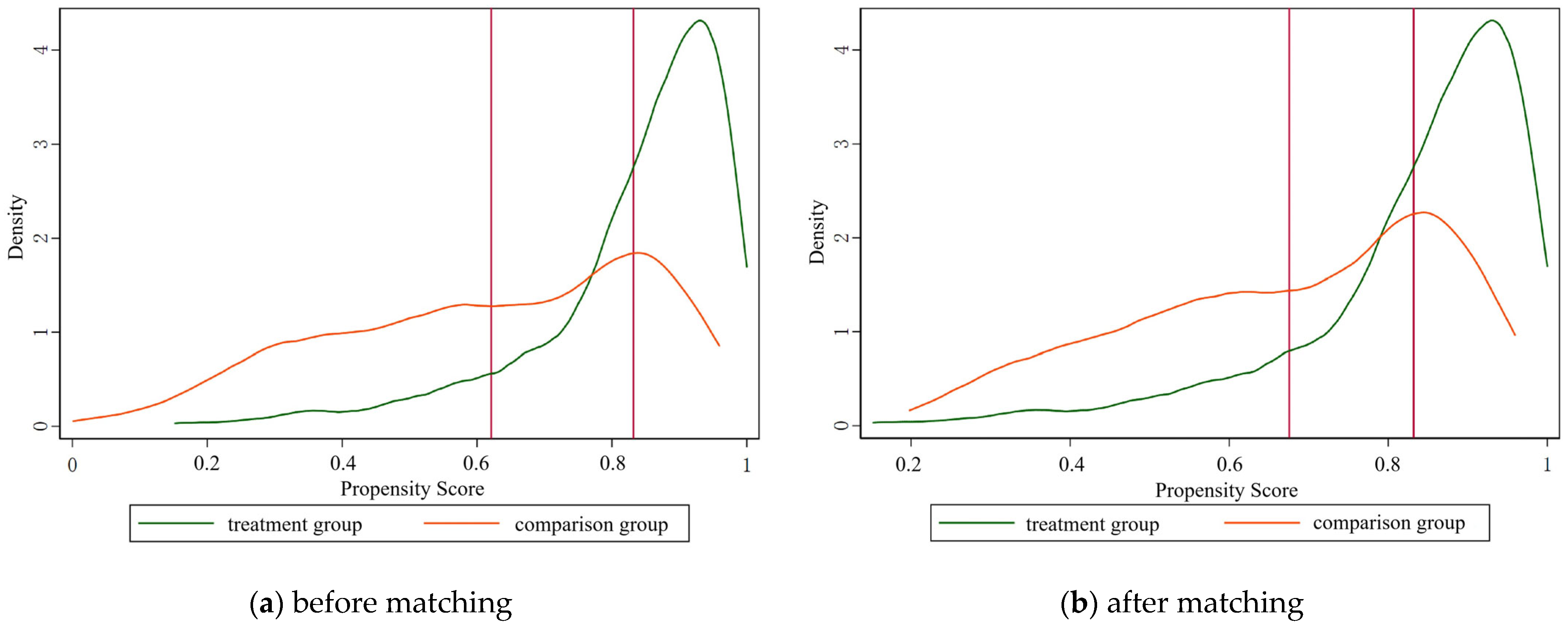
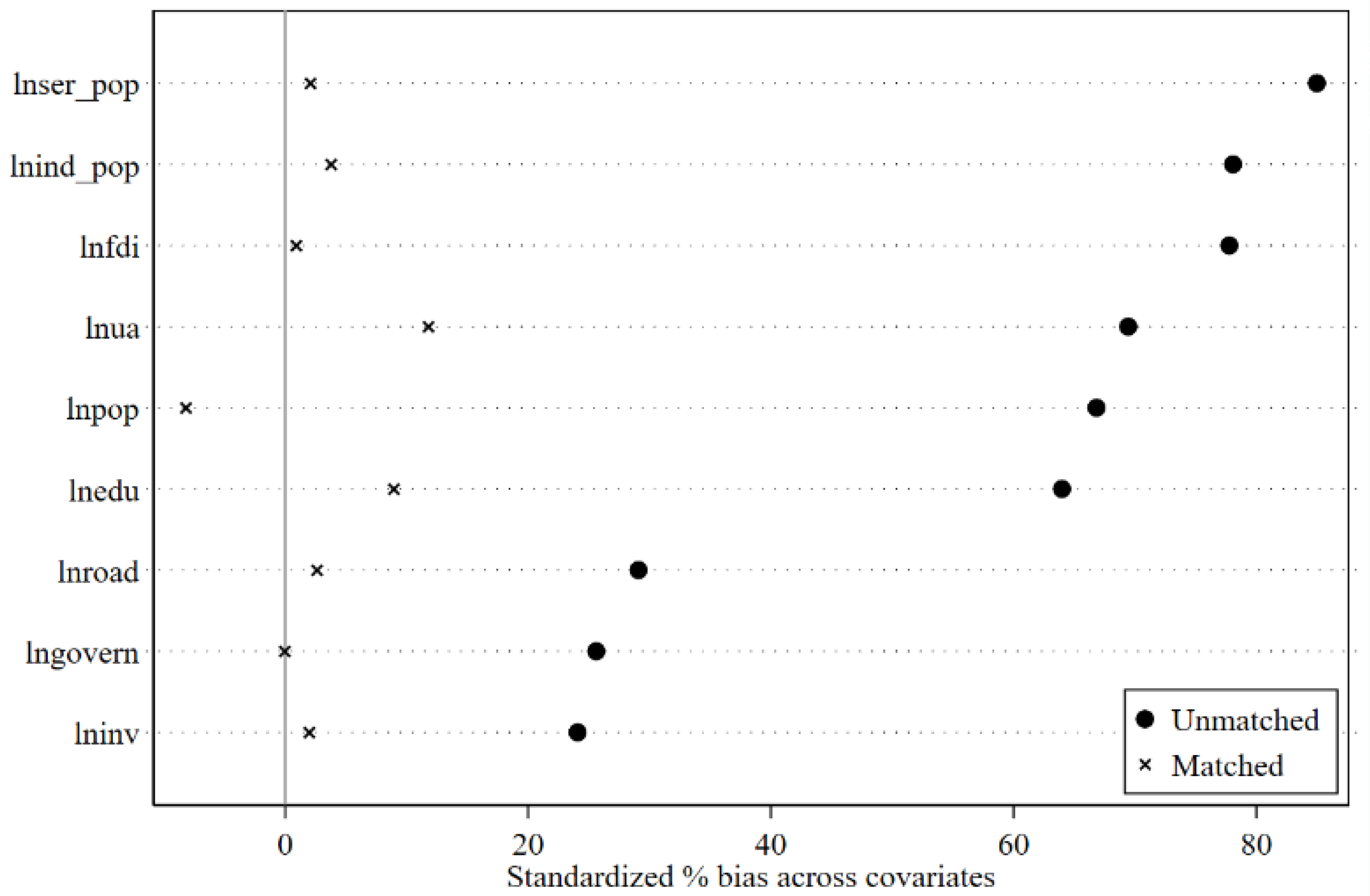
3.2. City Grouping Based on PSM

Before applying the DID model to analyze the intercity industrial distribution effects (IDEs) of China’s HSR, it is crucial to appropriately group the samples and address sample selection bias. Figure 2a,b show the P-score distribution functions for the treatment and comparison groups before and after matching, respectively, with the probability of HSR operation calculated using Equation (3). Before matching, the P-score probability density distribution differed significantly between the two groups. The treatment group’s distribution was concentrated and right-skewed, while the comparison group’s distribution was more dispersed (Figure 2a). After matching, as shown in Figure 2b, the mean value lines for both groups converge, indicating a closer alignment and similar characteristics. Figure 3 illustrates the propensity score distribution of the matched groups. The results reveal that 35 observations from 22 cities in the comparison group did not meet the matching criteria. These cities had an unusually high or low probability of being selected as HSR cities, resulting in a failure to match all samples. Consequently, these outlier observations, located at both ends of the kernel density curve, were excluded.

Table 3. Balance test of variables before and after PSM.

Variable	Unmatched (U)	Mean Value			% Reduction Bias	t-Test
	Matched (M)	T	C	% Bias		t	p > t
ln(pop)	U	5.87	5.51	56.00		11.08	0.00
	M	5.87	5.92	−7.00	87.50	−1.93	0.65
ln(ua)	U	4.38	3.97	52.00		9.43	0.00
	M	4.38	4.30	9.30	82.20	2.75	0.21
ln(inv)	U	16.10	15.64	23.30		4.32	0.00
	M	16.10	16.14	−2.20	90.70	−0.71	0.48
ln(govern)	U	14.85	14.59	43.90		7.98	0.00
	M	14.85	14.85	0.00	100.00	0.00	1.00
ln(fdi)	U	8.69	6.54	59.60		11.79	0.00
	M	8.69	8.68	0.40	99.40	0.12	0.91
ln(road)	U	6.71	6.31	25.00		4.53	0.00
	M	6.71	6.72	−1.10	95.60	−0.31	0.76
ln(edu)	U	10.50	9.233	64.0		12.61	0.01
	M	10.27	10.096	8.9	86.0	3.2	0.85
ln(ind_pop)	U	2.70	2.20	55.80		10.12	0.00
	M	2.70	2.65	5.20	90.60	1.48	0.14
ln(ser_pop)	U	2.87	2.54	59.50		10.93	0.00
	M	2.87	2.86	1.50	97.40	0.43	0.67

and Figure 4 present the detailed statistical information of covariables before and after PSM. The estimation bias (% bias) of all variables after matching is significantly reduced to less than 20%. Moreover, the t-test results of all variables after matching are insignificant, indicating no significant difference between the treatment group and the comparison group, which is suitable for further DID analysis.

3.3. Preliminary Judgment on Urban Industrial Agglomeration Effects of HSR

Due to the time span of the NPP/VIIRS dataset, this study examines 155 cities (68% of cities with HSR) that began HSR operation between 2012 and 2019. The changes in LA_GDP before and after HSR operation are calculated using the same time span. For instance, for Yantai, which first operated HSR in 2014, ΔLA_GDP = [(LA_GDP2015 + LA_GDP2016)/2] − [(LA_GDP2012 + LA_GDP2013)/2]; and for Huangshan, which began in 2015, ΔLA_GDP = [(LA_GDP2016 + LA_GDP2017 + LA_GDP2018)/3] − [(LA_GDP2012 + LA_GDP2013 + LA_GDP2014)/3]. This process is repeated for all 155 cities. Figure 5 shows the spatial distribution of ΔLA_GDP, with the natural breakpoint method dividing it into four levels. Cities with declining ΔLA_GDP are shown in red, with “Reduce I” declining more than “Reduce II”; cities with rising ΔLA_GDP are shown in blue, with “Increase II” rising more than “Increase I”.

“Increase I” and “Increase II” dominate the northeastern and eastern regions, while “Reduce I” predominates in the central region and “Reduce II” is mostly found in the western region. These results suggest that LA_GDP increased in the eastern, northeastern, and western high-administrative-level cities, while it decreased in the central and western regions. Therefore, the industrial effects of HSR are more concentrated in the eastern region and dispersed in the central and western regions, with high luminous intensity tertiary industry activities flowing from the central and western areas to the eastern region.

This pattern reflects China’s regional economic restructuring, where the central region has absorbed industrial transfers from developed areas. Provinces such as Shanxi, Anhui, and Henan have improved transportation with north–south Beijing–Guangzhou and Beijing–Haikou lines, as well as east–west Shanghai–Chengdu and Shanghai–Urumqi lines. In the early 21st century, labor-intensive industries like primary processing and assembly plants moved from the coastal east to the interior, attracted by lower resource costs and large domestic markets. However, the central region struggles to attract high-level talent, causing high-luminous-intensity tertiary industries to flow eastward. The only exceptions are cities like Yibin and Zhangjiajie, where tourism-related tertiary activities remain prominent. Meanwhile, eastern provinces such as Zhejiang, Jiangsu, Guangdong, and Fujian, benefiting from dense transportation networks, have successfully moved backward industries out and accelerated industrial upgrading.

In summary, from a spatial perspective, high-luminous-intensity tertiary industry activities primarily flow from the central and western regions to the eastern and northeastern regions, where they become more concentrated. These industries include producer services, consumer services, and public services. Further empirical analysis will be conducted based on these findings.

3.4. Results

3.4.1. The Impact of HSR on Urban Industrial Structure

Table 4. The intercity IDEs of HSR: baseline regression results.

Dependent Variable: LAGDP	(1)	(2)	(3)
DID	−0.101 ***	−0.0631 ***	−0.0580 **
	(−3.561)	(−2.733)	(−2.474)
ln(pop)			−0.0310
			(−0.647)
ln(ua)			−0.0187 *
			(−1.835)
ln(inv)			−0.00613
			(−0.423)
ln(govern)			−0.0118
			(−1.514)
ln(edu)			−0.0120 **
			(−2.050)
ln(fdi)			0.000555
			(0.172)
ln(road)			0.000678
			(0.0772)
Constant	YES	YES	YES
City Fixed Effect	NO	YES	YES
Time Fixed Effect	NO	YES	YES
Observations	2144	2144	2122
R2	0.06	0.04	0.12

Note: *, **, and *** indicate significance at the 10%, 5% and 1% levels, respectively.

presents the full-sample regression results of the DID model after successful matching. Column (1) shows the mixed regression results using the least square method for the entire sample. The results indicate that HSR’s impact on LA_GDP is negative and significant at the 1% level, demonstrating that without controlling for other factors, HSR inhibits the upgrading of urban industrial structure. In column (2), after controlling for both city and time fixed effects, the DID coefficient remains significant but decreases substantially in magnitude, which aligns with the expected outcome and confirms the appropriateness of the DID model. In column (3), after adding other control variables affecting economic development, the results show that HSR reduces LA_GDP by 5.8%. This suggests that the operation of HSR in China has led to a modest decline in the proportion of tertiary industry in HSR-connected cities’ economies, while simultaneously enhancing the presence of secondary industry. (It should be noted that this refers to industrial structure, rather than economic volume or per capita GDP, which may still increase). Other factors, such as urban built-up area and human capital stock, are negatively correlated with LA_GDP, with significance at the 10% and 5% levels, respectively. This may be explained by the fact that larger cities tend to take longer to achieve comprehensive industrial upgrading.

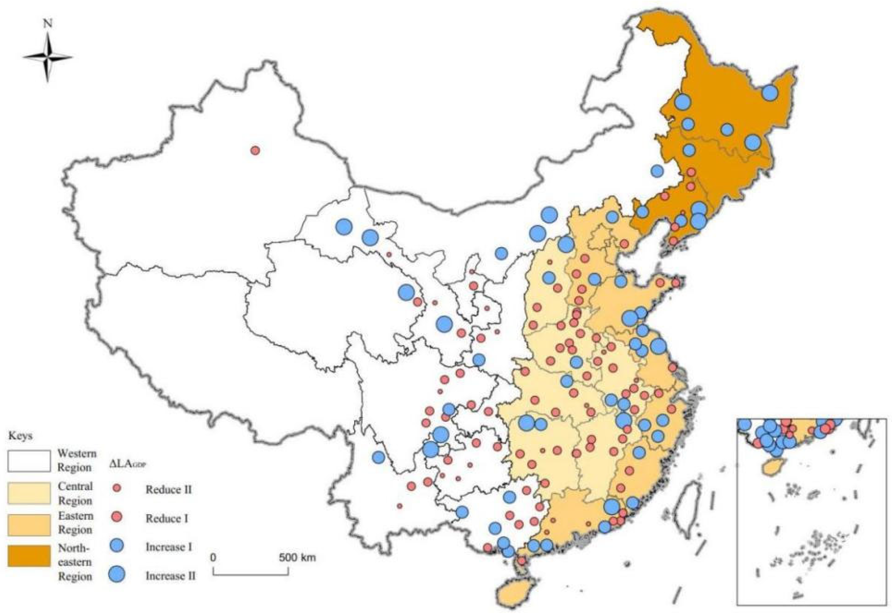
3.4.2. Intercity IDEs and Its Spatial Heterogeneity of HSR

(1)

Regional differentiation and influence mechanism analysis of IDEs of HSR

The analysis above demonstrates the national-level impact of HSR on urban industrial structure upgrading. Considering inter-regional heterogeneity, this section examines regional variations in HSR’s effect on industrial structure across the eastern, central, western, and northeastern regions. In

Table 5. Heterogeneous IDEs of HSR in different regions.

Dependent Variable: LAGDP	(1)	(2)	(3)	(4)	(5)	(6)	(7)	(8)
	Eastern Region	Central Region	Western Region	Northeastern Region	Eastern Region	Central Region	Western Region	Northeastern Region
DID	0.232	−1.586 ***	−1.932 **	3.672 **	0.321	−1.411 ***	−1.610 *	0.259
	(0.441)	(−3.552)	(−2.350)	(2.351)	(0.558)	(−2.841)	(−1.918)	(0.165)
ln(pop)					−16.38 ***	−1.965	1.709	−20.22 *
					(−3.414)	(−0.878)	(1.285)	(−1.740)
ln(ua)					0.0883	−0.515	−2.071 ***	−0.0144
					(0.356)	(−1.545)	(−3.770)	(−0.0239)
ln(inv)					−1.837 **	3.604 ***	0.391	−2.233 ***
					(−2.421)	(6.089)	(1.393)	(−2.918)
ln(govern)					2.211 **	−4.552 ***	−0.561 *	5.551 ***
					(2.236)	(−5.279)	(−1.739)	(2.816)
ln(edu)					−0.0511	−0.289	−0.208	0.0523
					(−0.368)	(−1.513)	(−1.045)	(0.179)
ln(fdi)					0.181	0.0529	−0.0641	−0.276 **
					(1.550)	(0.677)	(−0.629)	(−2.258)
ln(road)					−0.127	−0.168	0.175	0.0948
					(−1.397)	(−1.328)	(1.055)	(0.341)
Constant	YES	YES	YES	YES	YES	YES	YES	YES
City Fixed Effect	YES	YES	YES	YES	YES	YES	YES	YES
Time Fixed Effect	YES	YES	YES	YES	YES	YES	YES	YES
R2	0.001	0.022	0.009	0.023	0.044	0.096	0.047	0.173

Note: *, **, and *** represent significance at the 10%, 5%, and 1% levels, respectively.

(columns 1 to 4), the DID results are positive for the eastern and northeastern regions, and negative for the central and western regions. The significance levels are 1%, 5%, and 5% for the central, western, and northeastern regions, respectively. After controlling for additional variables, the signs of the HSR effects remain consistent, confirming the reliability of the results. The negative DID results in the central and western regions suggest that HSR has reduced the luminous intensity of economic activities and accelerated the outflow of tertiary industry activities. The decline in economic activities of the tertiary industries was more pronounced in the western region compared to the central region.

The covariate values for the regional regressions in the eastern and northeastern regions are shown in columns (5) and (8) of Table 5. Notably, the year-end population (pop) indicator is significantly negative. Previous studies have suggested a nonlinear relationship between population size and HSR effects [49]. Specifically, when the population exceeds a certain threshold, the HSR effects may become insignificant or even negative. Large cities with high populations tend to have larger industrial scales, often dominated by labor-intensive industries with low luminous efficiency, making industrial restructuring more challenging. The built-up area (ua) indicator is negative in both the central and western regions, but significant only in the western regions. This suggests that in less developed areas, cities with smaller urban scales are more likely to shift their economic development models and foster industrial upgrading. The fixed asset investment (inv) indicator is significantly negative in the eastern and northeastern regions, but significantly positive in the central region, with a notably higher coefficient. These results highlight the urban development potential in the central region, indicating that infrastructure improvements are needed to support industrial structure optimization. Lastly, the government public financial expenditures (govern) indicator is significantly positive in the eastern and northeastern regions but significantly negative in the central and western regions. This suggests that in the relatively underdeveloped central and western regions, an early focus on increasing expenditure for people’s livelihood may hinder the rapid industrial transformation and upgrading of cities in the short term.

The results in column (4) reveal positive industrial effects of HSR in the northeastern region, indicating that it has promoted the growth of tertiary industry employment. However, as shown in column (8), when additional variables are included, the regression result becomes insignificant, though it remains positive. Studies have shown that cities in the northeastern region are facing severe urban shrinkage, with issues such as population decline, economic recession, and urban decay, which hinder sustainable development [50]. To explore the role of HSR in the industrial development of these resource-depleted cities, this paper conducts a focused analysis. Using the number of employees in secondary and tertiary industries as the dependent variable, the regression results, presented in

Table 6. Regression results for the northeastern region.

	(1)	(2)
Dependent Variable	ind_pop	ser_pop
DID	−0.178 ***	−0.00455
	(−2.603)	(−0.185)
Other Constant Variables	YES	YES
City Fixed Effect	YES	YES
Time Fixed Effect	YES	YES
Observations	272	272
R2	0.491	0.090

Note: *** represent significance at the 1% levels, respectively.

, show that HSR operation inhibits the growth of the secondary industry in the northeastern region. A possible explanation is that HSR has accelerated the outflow of labor in these areas. However, the outflow effect on the tertiary industry is insignificant. Consequently, the intensity of economic activities in the secondary industry has declined in the northeastern region, resulting in a relative increase in the proportion of tertiary industry activities. Based on this, the northeastern region has not achieved a significant industrial structure upgrade.

(2)

The IDEs of HSR by city types and regions

In this study, the population of 290 cities at the end of 2019 is divided into four groups to analyze the intercity heterogeneity of HSR’s IDEs. Based on the Circular of the State Council on Adjusting the Standard for the Classification of City Scales ([2014] No. 51), Chinese cities are categorized into small and medium-sized cities, metropolises, megacities, and supercities, with populations of 1 million, 3 million, 5 million, and 10 million, respectively. Nationwide and regional regressions are conducted, and the results are presented in

Table 7. IDEs of HSR by city by region (coefficients of DID regression).

Dependent Variable: LAGDP	(1)	(2)	(3)	(4)
	Medium and Small Cities	Metropolis	Megacities	Supercities
Nationwide	−0.0239	−0.152 ***	0.0138 *	−0.102
	(−0.805)	(−3.121)	(0.404)	(−1.015)
Eastern	0.685	0.200	0.948 **	0.398 *
	(1.538)	(0.368)	(2.291)	(1.835)
Central	−0.196	−0.484	0.236	−1.252 *
	(−0.373)	(−0.950)	(0.412)	(−1.747)
Western	−0.936 **	−1.921 ***	−1.507 ***	−1.954 ***
	(−2.015)	(−3.417)	(−2.913)	(−3.054)
Northeastern	0.106	−1.121 *	0.839	0.629
	−0.154	(−1.669)	−1.591	−0.669
Other Control Variables	YES	YES	YES	YES
City Fixed Effect	YES	YES	YES	YES
Time Fixed Effect	NO	NO	NO	NO

Note: *, **, and *** represent significance at the 10%, 5%, and 1% levels, respectively.

(only the core DID variable is retained).

The nationwide regression results show a positive effect for the megacities group and an inhibiting effect for the metropolises group, significant at the 1% and 10% levels, respectively. As the population expands from metropolises (3~5 million) to megacities (5~10 million), the industrial structure upgrading effect of HSR shifts from negative to positive. However, when cities exceed 10 million in population, this effect becomes insignificant, similar to the HSR’s effect on land-use intensity [49]. This may be because supercities have a more solid industrial base, making structural changes difficult.

Full-sample regression results at the national level indicate that HSR has facilitated the flow of high luminous intensity economic activities from metropolises to megacities. The results from the four regions show that supercities and megacities in the eastern region are the primary destinations for the inflow of tertiary industry economic activities, while metropolises, megacities, and supercities in the central and western regions are the main sources of outflow. Comparing the megacities and supercities in the eastern region, the agglomeration of tertiary industries is most prominent in megacities (with a DID coefficient of 0.948, which is greater than that of the supercities). This suggests that the agglomeration effect of HSR on tertiary industries is stronger in megacities than in supercities, aligning with the population scale hypothesis. A key reason for this is that high land prices in megacities have increased the location costs for tertiary industries. The regression results in Table 5, which show weak agglomeration in the eastern region due to HSR, support the conclusion that tertiary industries are mainly flowing into megacities and supercities in the eastern region. However, the agglomeration effect in smaller cities in the eastern region is less pronounced. In the northeastern region, there is an outflow of tertiary industries from metropolises, but no significant inflow, indicating that tertiary industries from the northeastern region are also migrating to the eastern region. Overall, the operation of HSR promotes the agglomeration of tertiary industries in China, particularly in megacities and supercities in the eastern region, with a stronger effect in megacities.

3.4.3. The Sectoral Differences of the IDEs of HSR

Based on the analysis above, HSR promotes the agglomeration of tertiary industries in a few megacities, contributing to industrial structure upgrading. Given the diversity of economic activities in service industries, further analysis is required to determine which clusters are influenced by HSR. Therefore, the service industries are divided into producer, consumer, and public service sectors, with the number of employees in each sector as the dependent variable, to further analyze the differential IDEs across these sectors.

The results in

Table 8. Regression results by service industry sector.

	(1)	(2)	(3)
	Producer Service	Consumer Services	Public Services
DID	0.221 ***	−0.149	0.0554
	(7.982)	(−3.905)	(4.028)
ln(pop)	−0.0181	0.104 *	−0.0195
	(−0.153)	(1.853)	(−0.305)
ln(ua)	0.0248	−0.0170	0.00829
	(1.609)	(−1.342)	(0.861)
ln(inv)	0.0743 **	0.0875 ***	0.0129
	(2.416)	(3.586)	(0.784)
ln(govern)	0.0683	−0.0362 *	0.0248 *
	(1.568)	(−1.807)	(1.841)
Other Control Variables	YES	YES	YES
City Fixed Effect	YES	YES	YES
Time Fixed Effect	YES	YES	YES
Observations	2192	2192	2192
R2	0.171	0.042	0.057

Note: *, **, and *** represent significance at the 10%, 5%, and 1% levels, respectively.

show that only producer services are significantly promoted by HSR (at the 1% significance level), while consumption and public services are not. This finding is consistent with the studies of Yang et al. [14] and Shao et al. [37] Producer services depend on human resources, information, knowledge, and other inputs, and are characterized by high specialization and trade [51]. HSR, with its speed and comfort, meets the high demand for mobile elements in these industries, thus exerting a significant impact, causing them to concentrate in HSR cities.

Lowry [52] classifies urban industries into basic and retail sectors. Basic sectors refer to export industries or economic activities whose products or services are sold outside the city, bringing income to the urban economy. These sectors form the city’s economic foundation. In contrast, retail sectors include industries like catering and retail that support the city’s daily operations. Consumer and public service industries largely fall under retail sectors, serving local needs. Their development is primarily driven by local economic demand and is less sensitive to inter-regional transportation.

Table 9. Regression results by sub-sectors of the three major service industry.

Producer Services						Consumer Services
	Transportation, Warehousing, and Postal Service Industry	Information Transmission, Software, and Information Technology Service Industry	Financial Industry	Leasing and Business Service Industry	Science Research and Technology Service Industry	Real Estate Industry	Residential Services, Repairs, and Other Services
DID	0.523 ***	0.082	0.160 ***	0.375 ***	−0.010	0.252 ***	0.137
	(0.060)	(0.057)	(0.020)	(0.057)	(0.026)	(0.045)	(0.093)
Other Control Variables	YES	YES	YES	YES	YES	YES	YES
City Fixed Effect	YES	YES	YES	YES	YES	YES	YES
Time Fixed Effect	YES	YES	YES	YES	YES	YES	YES
Observations	2183	2184	2191	2191	2188	2189	2173
R2	0.157	0.008	0.106	0.123	0.052	0.107	0.048
Consumer Services				Public Services
	Accommodation and catering industry	Culture, sports, and entertainment industry	Wholesale and retail industry	Public administration, social security, and social organizations	Water conservancy, environmental and public facilities management	Health and social work	Education
DID	−0.810 ***	0.006	0.018	0.102 ***	−0.088	0.124 ***	0.018
	(0.072)	(0.030)	(0.045)	(0.013)	(0.035)	(0.018)	(0.016)
Other Control Variables	YES	YES	YES	YES	YES	YES	YES
City Fixed Effect	YES	YES	YES	YES	YES	YES	YES
Time Fixed Effect	YES	YES	YES	YES	YES	YES	YES
Observations	2189	2187	2184	2183	2188	2188	2188
R2	0.184	0.019	0.052	0.112	0.010	0.211	0.032

Note: *** represent significance at the 1% levels, respectively.

presents the regression results based on the DID model, using the number of employees in 14 service industry categories as dependent variables. Positive industrial effects are observed in the transportation, warehousing, postal service, financial, leasing, business services within producer services, and real estate within consumer services. The operation of HSR directly influences the expansion of local transportation and warehousing infrastructure, leading to an increase in employment in these sectors. Previous studies have shown that housing prices around HSR stations have risen [53], stimulating growth in the financial and leasing industries related to real estate. In the public service sectors, the DID coefficients for public administration, social security, social organizations, and health services are significantly positive, suggesting that HSR promotes urban public service improvements and enhances health and social security systems to a certain extent.

It is worth noting that a significant negative effect of HSR has been identified in the accommodation and catering industries. On the national level, HSR appears to reduce the average number of employees in these industries, contrary to the traditional view that HSR promotes tourism-related sectors [12]. Two possible reasons for this are as follows. First, producer service industries are often information- and knowledge-intensive, highly specialized, and trade-oriented, requiring frequent exchanges and interactions. Their high mobility generates joint demand for accommodation and catering services. As HSR has concentrated producer service industries in a few metropolises, it has simultaneously hindered the growth of accommodation and catering in other cities. Second, HSR has amplified the polarization of tourism across the country. Song et al. [8] note that cities such as Beijing, Shanghai, Guangzhou, and Wuhan have become super tourist hubs. As a result, accommodation and catering industries have declined in other cities, with a siphoning effect occurring in most HSR cities, leading to negative overall measurements. Thus, HSR has intensified the siphon effect rather than the spillover effect of tourism from a few supercities or megacities.

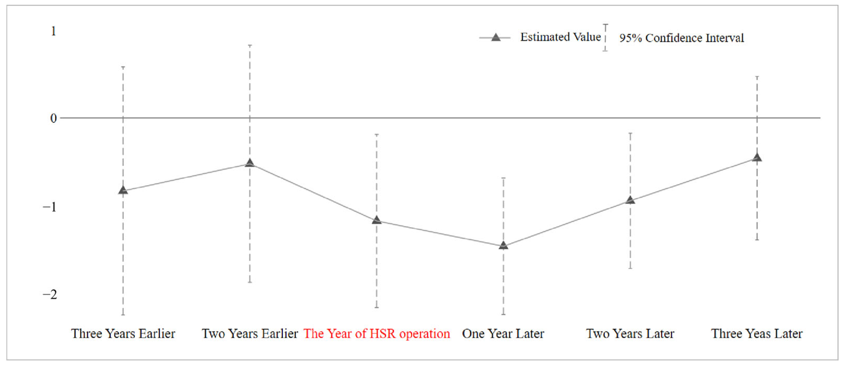
4. Parallel Trend Tests

The premise of the DID model is that there are no systematic differences between the treatment and comparison groups before the operation of HSR, meaning that the LA_GDP of both groups follows the same trend over time. To validate the parallel trend assumption of the model, a falsification test was conducted using event study methodology, following He et al. [54] and Qin [55]. This method examines the policy effect by setting multiple years of HSR operation. Assuming the actual operation year of HSR is T, considering data availability and statistical efficiency [6], this study defines the operation years as T-3 to T+3 for model testing (see Equation (4)):

$${LAGDP}_{it}=\alpha +\sum _{L-T\ne -1}\left({\alpha }_1\times DID\right)+\sum _{\mathrm{i}=1}^N{\mathsf{\gamma }}_{\mathrm{j}}{X}_{it}+{\mu }_i+{\lambda }_t+{\epsilon }_{it}.$$

(4)

The operation year of HSR is denoted as L, and the other variables (except α₁) remain the same as in the previous model. The value of parameter α₁, derived from the regression analysis of Equation (4), is presented in Figure 6, where the horizontal axis represents the relative time of HSR operation. The estimated values of α₁ for two and three years before HSR operation are close to zero (with “one year earlier” as the base time of the model [56]. Additionally, no values fall outside the 95% confidence interval, suggesting that the difference in HSR’s industrial effect does not reject the null hypothesis, thus confirming the validity of the parallel trend assumption.

5. Discussion

5.1. Rationality of the Results

To establish a consistent basis for a long time series of data, this study employs an index, LA_GDP, based on NTL to characterize changes in urban industrial structure. While Section 3.1 demonstrates that different industries exhibit varying NTL effects, a potential concern is the source of NTL, as it may originate from both residential and economic activities. However, industries differ in their capacity to absorb employment, leading to significant variations in the number of workers per unit of GDP. Consequently, the intensity of residential NTL per unit of GDP also varies across industries. Industry serves as the foundation of a city, shaping many of its characteristics and accounting for disparities between cities. We acknowledge that external factors, such as weather, may introduce unavoidable biases even after calibration. Therefore, the effects of HSR on the development of the urban tertiary industry may not be entirely precise. However, the observed trends are reasonable and provide valuable insights for the further planning and layout of HSR.

This paper concludes that the flow of producer services to a small number of megacities and supercities does not imply a decline in the economies of other cities. Our focus is on the agglomeration effect of HSR on industries, rather than its impact on overall urban economic development. Therefore, it does not contradict existing research, such as that by Niu and Xin [49], which shows that HSR stations have significantly increased economic activity intensity in surrounding areas. Different from this kind of existing research which focus on the overall effect of HSR on economic volume, this study aims to identify the impact of HSR on industrial structure of a city. The changes in industrial structure of a city, especially those small and medium-sized cities, due to the operation of HSR simply do not mean a general decline/growth in economic activity.

5.2. Reasons for HSR’s Effects on Industrial Distribution

This research concludes that HSR promotes the flow of urban tertiary industries, particularly producer service industries, to megacities and supercities. Previous studies provide possible explanations for this trend. Sassen (2001) argued that, in the process of urban space development, manufacturing initially concentrates in core cities. As industrial scale expands and land prices rise, businesses relocate factories to surrounding areas. Meanwhile, producer industries, which typically occupy smaller spaces (such as finance and law, where each staff member requires minimal office space), tend to agglomerate in core cities, and these industries benefit from proximity [57,58]. Chen [59] posits that high-speed rail (HSR) induces a time-space compression effect by reducing commuting times, thereby enhancing the capacity of megacities and supercities to attract economic resources from surrounding regions. Dong [12] further demonstrates that HSR is especially advantageous for industries reliant on human flow and market interactions—characteristics that define producer services, which depend on high-end markets and industrial agglomeration. This study corroborates these findings, highlighting that producer services are particularly responsive to the connectivity and agglomeration benefits provided by HSR. The operation of HSR enhances inter-city connectivity and strengthens urban integration, facilitating the flow of secondary industries to surrounding cities and the concentration of producer services in megacities and supercities.

5.3. Policy Implications

Based on impacts of HSR on industrial distribution, the following principles should be followed in addressing the effects of HSR on industries:

(1)

Transformation of the traditional mindset of blindly relying on the operation of HSR to pursuing economic development. In September 2019, China issued the “Outline for Building a Powerful Transportation Country”, aiming to further develop HSR technology and deploy trains capable of reaching speeds of 600 km per hour. Amid this wave of high-speed rail construction, many small cities have also built HSR stations. These small cities, lacking economic development momentum, view HSR construction as an opportunity for economic growth and develop new HSR city centered around HSR stations. However, the aforementioned results indicate that the impact of HSR on urban development differs depending on the city’s size and industrial structure. Cities should comprehensively consider their own industrial structure and the cities they are connected to through HSR, formulating development policies tailored to local conditions. For example, for small cities dominated by manufacturing, the opening of HSR connecting them to large cities will facilitate the transfer of secondary industries from large cities. On the other hand, for small cities primarily focused on the service industry, their connection to large cities via HSR may lead to the outflow of their service industries. This corroborates Faber’s [60] view that high-speed rail construction is not a game without losers. In particular, remote counties should remain calm and carefully assess the costs and benefits of high-speed rail construction when facing new rounds of railway planning [61].

(2)

Due to the varying impacts of high-speed rail on different cities, each HSR city needs to formulate distinct land use policies to address the impact of HSR on its industries. Compared to manufacturing, producer services require less space and can be highly concentrated within a single building (for instance, a lawyer can operate from just one office space). This enables producer services to adapt to high land prices. Additionally, spatial agglomeration further promotes the development of producer services. In contrast, manufacturing typically requires substantial land for factory construction. In order to avoid the high land costs in large cities, enterprises choose to relocate to surrounding smaller cities. Therefore, for large cities, they can develop high-rise office spaces and convention centers to facilitate the agglomeration of producer services and face-to-face exchanges. For smaller cities, in order to attract manufacturing transfers, they need to implement relatively lenient land policies to facilitate factory construction.

(3)

It is necessary to consider both the industrial situation of the city itself and that of the cities connected through high-speed rail when making policy decisions. The ultimate reason for the varying impacts of HSR on urban industries lies in the differences in industrial structure and scale among cities. HSR makes cities more closely connected and also leads to a clearer division of labor among them. Decision-makers need to take comprehensive consideration of the situation of the HSR city and the cities it is connected to. Small cities and those located in the central and western regions, the central government should accelerate the construction of the high-speed rail network to promote economic connections with developed cities and reduce regional (urban) disparities. At the same time, non-central cities should choose their development directions based on their distances from the nearest central cities [62]. Each city may face different scenarios: being connected to larger cities, smaller cities, both larger and smaller cities simultaneously, or cities of similar types. Previous discussions have addressed the potential flow directions of manufacturing and service industries. However, when an HSR city is connected to similar cities, decision-makers need to clarify its comparative advantages, make joint decisions, rationalize its division of labor, and pursue differentiated development. This involves coordinated intercity development and requires overall decision-making by a higher-level government to mitigate the negative impacts of high-speed rail, such as the decline in tertiary industries in medium-sized cities or the exacerbation of disparities between megacities and smaller urban areas.

5.4. Limitations and Future Directions

Several existing limitations in this study point to future wok. First, further research on the impact of HSR on individual cities is required. This paper analyzes the impact of HSR on intercity industrial distribution, with a focus on general trends rather than specific cities. While this study concludes that HSR promotes the flow of tertiary industries to the eastern region, it acknowledges that megacities or supercities in the western underdeveloped region may also attract such industries. Similarly, small and medium-sized cities in the eastern developed region may experience an outflow of economic activities. To fully understand the impact of HSR on specific cities, targeted research for individual cities is essential. Second, as nightlight data only reflect industrial change of each city, it does not reflect the industrial transfer routes, i.e., the origin and destination, future studies could be expanded by incorporating data on the migration of economic activities, such as population movement (with origin and destination), POI data, mobile signaling data, and the spatiotemporal distribution of businesses. Additionally, urban environmental factors, such as latitude, longitude, light, and temperature, may influence NTL intensity. Including relevant control variables to account for these effects is another important area for further exploration.

6. Conclusions

In this study, we proposed a novel approach to identify the intercity IDEs of HSR at different levels based on NTL data. The approach provides a new way to identify the effects of HSR on both secondary and tertiary industries on broad scales and for long periods of time. The case of China’s HSR shows that the approach performed well and has potential for widespread use elsewhere. The results show that, overall, HSR has promoted the development of the tertiary industry in HSR cities, but it has only facilitated agglomeration of tertiary industry towards a few megacities and supercities while dispersing secondary industries from those cities. This kind of industrial effects of HSR is more pronounced in the supercities in the eastern region. Consequently, in most medium and small cities, the proportion of the tertiary industry decreased, and that of the secondary industry increased. Furthermore, at the regional level, HSR has facilitated the flow of tertiary industries from the central, western, and northeastern economic regions to cities in the eastern economic region, while the central region has absorbed secondary industries relocated from the eastern and northeastern regions. In addition, the agglomeration effects of HSR are most significantly in the producer service industries. Positive effects are identified in transportation, warehousing, postal services, financial, leasing, and business services within producer services, as well as in real estate within consumer services. However, HSR exerts an inhibiting effect on tourism-related industries, specifically accommodation and catering, highlighting its role in enhancing the siphon effect of a few supercities and megacities on tourism from other cities.

References

- Zhang, W.; Ding, N.; Lv, G. Study on the influence of high-speed railway on the consumption space of Yangtze River Delta cities. Econ. Geogr. 2012, 32, 1–6. [Google Scholar]
- He, C.; Zhu, S. The principle of relatedness in China’s regional industrial development. Acta Geogr. Sin. 2020, 75, 2684–2698. [Google Scholar]
- Wang, Y.; Ni, P. Economic growth spillover and spatial optimization of high-speed railway. China Ind. Econ. 2016, 2, 21–36. [Google Scholar]
- Ravenstein, E. The laws of migration, part I. J. Stat. Soc. Lond. 1885, 48, 167–235. [Google Scholar] [CrossRef]
- Duranton, G.; Turner, M.A. Urban growth and transportation. Rev. Econ. Stud. 2012, 79, 1407–1440. [Google Scholar] [CrossRef]
- Lin, Y. Travel costs and urban specialization patterns: Evidence from China’s high speed railway system. J. Urban Econ. 2017, 98, 98–123. [Google Scholar] [CrossRef]
- Li, H.C.; Tjia, L.; Hu, S. Agglomeration and equalization effect of high-speed railway on cities in China. J. Quant. Tech. Econ. 2016, 11, 127–143. [Google Scholar]
- Song, W.; Zhu, X.; Zhu, Y.; Kong, C.; Shi, Y.; Gu, Y. The impacts of high-speed railways for different scale cities. Econ. Geogr. 2015, 35, 57–63. [Google Scholar]
- Swann, D. The Economics of the Common Market; Penguin Books: London, UK, 1992. [Google Scholar]
- Yu, H.; Jiao, J.; Houston, E.; Peng, Z.R. Evaluating the relationship between rail transit and industrial agglomeration: An observation from the Dallas-Fort Worth region, TX. J. Transp. Geogr. 2018, 67, 33–52. [Google Scholar] [CrossRef]
- Charnoz, P.; Lelarge, C.; Trevien, C. Communication costs and the internal organization of multi-plant businesses: Evidence from the impact of the French high-speed rail. Econ. J. 2018, 128, 949–994. [Google Scholar] [CrossRef]
- Dong, X. High-speed railway and urban sectoral employment in China. Transp. Res. Part A Policy Pract. 2018, 116, 603–621. [Google Scholar] [CrossRef]
- Tierney, S. High-speed rail, the knowledge economy and the next growth wave. J. Transp. Geogr. 2012, 22, 285–287. [Google Scholar] [CrossRef]
- Yang, L.; Hu, L.; Shang, P. Estimating the impacts of high-speed rail on service industry agglomeration in China: Advanced modeling with spatial difference-in-difference models and propensity score matching. J. Transp. Econ. Policy 2021, 55, 16–35. [Google Scholar]
- Monzón, A.; López, E.; Ortega, E. Has HSR improved territorial cohesion in Spain? An accessibility analysis of the first 25 years: 1990–2015. Eur. Plan. Stud. 2019, 27, 513–532. [Google Scholar] [CrossRef]
- Chang, Z.; Diao, M.; Jing, K.; Li, W. High-speed rail and industrial movement: Evidence from China’s greater bay area. Transp. Policy 2021, 112, 22–31. [Google Scholar] [CrossRef]
- Zhou, Z.; Zhang, A. High-speed rail and industrial developments: Evidence from house prices and city-level GDP in China. Transp. Res. Part A Policy Pract. 2021, 149, 98–113. [Google Scholar] [CrossRef]
- Yu, B.; Wang, C.; Gong, W.; Chen, Z.; Shi, K.; Wu, B.; Hong, Y.; Wu, J. Nighttime light remote sensing and urban studies: Data, methods, applications, and prospect. Natl. Remote Sens. Bull. 2021, 25, 342–364. [Google Scholar] [CrossRef]
- Tripathy, B.R.; Tiwari, V.; Pandey, V.; Elvidge, C.D.; Rawat, J.S.; Sharma, M.P.; Prawasi, R.; Kumar, P. Estimation of urban population dynamics using DMSP-OLS night-time lights time series sensors data. IEEE Sens. J. 2017, 17, 1013–1020. [Google Scholar] [CrossRef]
- Dai, Z.; Hu, Y.; Zhao, G. The suitability of different nighttime light data for GDP estimation at different spatial scales and regional levels. Sustainability 2017, 9, 305. [Google Scholar] [CrossRef]
- Wu, J.; Wang, Z.; Li, W.; Peng, J. Exploring factors affecting the relationship between light consumption and GDP based on DMSP/OLS nighttime satellite imagery. Remote Sens. Environ. 2013, 134, 111–119. [Google Scholar] [CrossRef]
- Li, X.; Xu, H.; Chen, X.; Li, C. Potential of NPP-VIIRS nighttime light imagery for modeling the regional economy of China. Remote Sens. 2013, 5, 3057–3081. [Google Scholar] [CrossRef]
- Shi, K.; Chen, Y.; Yu, B.; Xu, T.; Yang, C.; Li, L.; Huang, C.; Chen, Z.; Liu, R.; Wu, J. Detecting spatiotemporal dynamics of global electric power consumption using DMSP-OLS nighttime stable light data. Appl. Energy 2016, 184, 450–463. [Google Scholar] [CrossRef]
- Song, X.; Chen, Y.; Li, K. Analyzing spatiotemporal variation modes and industry-driving force research using VIIRS nighttime light in China. Remote Sens. 2020, 12, 2785. [Google Scholar] [CrossRef]
- Han, X.; Tana, G.; Qin, K.; Letu, H. Estimating industrial structure changes in China using DMSP-OLS night-time light data during 1999–2012. Int. Arch. Photogramm. Remote Sens. Spat. Inf. Sci. 2018, 42, 9–15. [Google Scholar] [CrossRef]
- Ghosh, T.; Anderson, S.; Powell, R.L.; Sutton, P.C.; Elvidge, C.D. Estimation of Mexico’s informal economy and remittances using nighttime imagery. Remote Sens. 2009, 1, 418–444. [Google Scholar] [CrossRef]
- Zhao, N.; Currit, N.; Samson, E. Net primary production and gross domestic product in China derived from satellite imagery. Ecol. Econ. 2011, 70, 921–928. [Google Scholar] [CrossRef]
- Li, X.; Zheng, X.; Yuan, T. Knowledge mapping of research results on DMSP/OLS nighttime light data. J. Geo-Inf. Sci. 2018, 20, 351–359. [Google Scholar]
- Elvidge, C.D.; Ziskin, D.; Baugh, K.E.; Tuttle, B.T.; Ghosh, T.; Pack, D.W.; Erwin, E.H.; Zhizhin, M. A fifteen years record of global natural gas flaring derived from satellite data. Energies 2009, 2, 595–622. [Google Scholar] [CrossRef]
- Gibson, J.; Olivia, S.; Boe-Gibson, G.; Li, C. Which night lights data should we use in economics, and where? J. Dev. Econ. 2021, 149, 102602. [Google Scholar] [CrossRef]
- Wu, Y.; Shi, K.; Yu, B.; Li, C. Analysis of the Impact of Urban Sprawl on Haze Pollution Based on the NPP-VIIRS Nighttime Light Remote Sensing Data. Geomat. Inf. Sci. Wuhan Univ. 2021, 46, 777–789. [Google Scholar]
- Pan, W.; Fu, H.; Zheng, P. Regional poverty and inequality in the Xiamen-Zhangzhou-Quanzhou city cluster in China based on NPP/VIIRS night-time light imagery. Sustainability 2020, 12, 2547. [Google Scholar] [CrossRef]
- Zhao, J.; Ji, G.; Yue, Y.; Lai, Z.; Chen, Y.; Yang, D.; Yang, X.; Wang, Z. Spatio-temporal dynamics of urban residential CO2 emissions and their driving forces in China using the integrated two nighttime light datasets. Appl. Energy 2019, 235, 612–624. [Google Scholar] [CrossRef]
- Jiao, J.; Wang, J.; Jin, F.; Wang, H. Impact of high-speed rail on inter-city network based on the passenger train network in China. Acta Geogr. Sin. 2016, 71, 265–280. [Google Scholar]
- Krugman, P. Increasing returns and economic geography. J. Political Econ. 1991, 99, 483–499. [Google Scholar] [CrossRef]
- Donaldson, D.; Hornbeck, R. Railroads and American economic growth: A “market access” approach. Q. J. Econ. 2016, 131, 799–858. [Google Scholar] [CrossRef]
- Shao, S.; Tian, Z.; Yang, L. High speed rail and urban service industry agglomeration: Evidence from China’s Yangtze River Delta region. J. Transp. Geogr. 2017, 64, 174–183. [Google Scholar] [CrossRef]
- Wang, L.; Acheampong, R.A.; He, S. High-speed rail network development effects on the growth and spatial dynamics of knowledge-intensive economy in major cities of China. Cities 2020, 105, 102772. [Google Scholar] [CrossRef]
- Chang, Z.; Zheng, L. High-speed rail and the spatial pattern of new firm births: Evidence from China. Transp. Res. Part A Policy Pract. 2022, 155, 373–386. [Google Scholar] [CrossRef]
- Lu, J. The performance of performance-based contracting in human services: A quasi-experiment. J. Public Adm. Res. Theory 2016, 26, 277–293. [Google Scholar]
- Rosenbaum, P.R.; Rubin, D.B. The central role of the propensity score in observational studies for causal effects. Biometrika 1983, 70, 41–55. [Google Scholar] [CrossRef]
- Heckman, J.J.; Ichimura, H.; Smith, J.A.; Todd, P. Characterizing Selection Bias Using Experimental Data; National Bureau of Economic Research: Cambridge, MA, USA, 1998. [Google Scholar]
- Chen, Q. Advanced Econometrics and Stata Applications; Higher Education Press: Beijing, China, 2014. [Google Scholar]
- Shi, D.; Ding, H.; Wei, P.; Liu, J. Can smart city construction reduce environmental pollution. China Ind. Econ. 2018, 6, 117–135. [Google Scholar]
- Wang, X.; Bu, B. International export trade and enterprise innovation—Research based on a quasi-natural experiment of CR express. China Ind. Econ. 2019, 10, 80–98. [Google Scholar]
- Xie, S.; Fan, P.; Wan, Y. Improvement and application of classical PSM-DID model. Stat. Res. 2021, 38, 146–160. [Google Scholar]
- GB/T4754-2017; National Economic Industry Classification. National Bureau of Statistics of China: Beijing, China, 2017.
- Li, P.; Fu, Y.; Zhang, Y. Can the productive service industry become new momentum for China’s economic growth. China Ind. Econ. 2017, 12, 5–21. [Google Scholar]
- Niu, F.; Xin, Z. Spillover effect of China’s railway stations and its spatial differentiation: An empirical study based on nighttime light datasets. Geogr. Res. 2021, 40, 2796–2807. [Google Scholar]
- Yang, Y.; Wu, J.; Wang, Y.; Huang, Q.; He, C. Quantifying spatiotemporal patterns of shrinking cities in urbanizing China: A novel approach based on time-series nighttime light data. Cities 2021, 118, 103346. [Google Scholar] [CrossRef]
- Zhao, M.; Liu, X.; Derudder, B.; Zhong, Y.; Shen, W. Mapping producer services networks in mainland Chinese cities. Urban Stud. 2015, 52, 3018–3034. [Google Scholar] [CrossRef]
- Lowry, I.S. A Model of Metropolis; RAND Corporation: Santa Monica, CA, USA, 1964. [Google Scholar]
- Diao, M. Does growth follow the rail? The potential impact of high-speed rail on the economic geography of China. Transp. Res. Part A Policy Pract. 2018, 113, 279–290. [Google Scholar] [CrossRef]
- He, G.; Pan, Y.; Tanaka, T. The short-term impacts of COVID-19 lockdown on urban air pollution in China. Nat. Sustain. 2020, 3, 1005–1011. [Google Scholar] [CrossRef]
- Qin, Y. ‘No county left behind?’ The distributional impact of high-speed rail upgrades in China. J. Econ. Geogr. 2017, 17, 489–520. [Google Scholar] [CrossRef]
- Beck, T.; Levine, R.; Levkov, A. Big bad banks? The winners and losers from bank deregulation in the United States. J. Financ. 2010, 65, 1637–1667. [Google Scholar] [CrossRef]
- Niu, F.; Yang, X.; Wang, F. Urban agglomeration formation and its spatiotemporal expansion process in China: From the perspective of industrial evolution. Chin. Geogr. Sci. 2020, 30, 532–543. [Google Scholar] [CrossRef]
- Sassen, S. The Global City: New York, London, Tokyo; Princeton University Press: Princeton, NJ, USA, 2001. [Google Scholar]
- Chen, C.-L. Reshaping Chinese space-economy through high-speed trains: Opportunities and challenges. J. Transp. Geogr. 2012, 22, 312–316. [Google Scholar] [CrossRef]
- Faber, B. Trade integration, market size, and industrialization: Evidence from China’s national trunk highway system. Rev. Econ. Stud. 2014, 81, 1046–1070. [Google Scholar] [CrossRef]
- Zhang, J. High-speed rail construction and county economic development: The research of satellite light data. China Econ. Q. 2017, 16, 1533–1562. [Google Scholar]
- Li, Z.; Wang, Q.; Cai, M.; Wong, W.-K. Impacts of high-speed rail on the industrial developments of non-central cities in China. Transp. Policy 2023, 134, 203–216. [Google Scholar] [CrossRef]