Modifying NISAR’s Cropland Area Algorithm to Map Cropland Extent Globally

 , , , , ,
  and
and
Abstract
1. Introduction
2. Materials and Methods
2.1. Data
2.1.1. Sentinel-1 Data and Processing
2.1.2. Reference Agricultural Data
2.2. Methodology
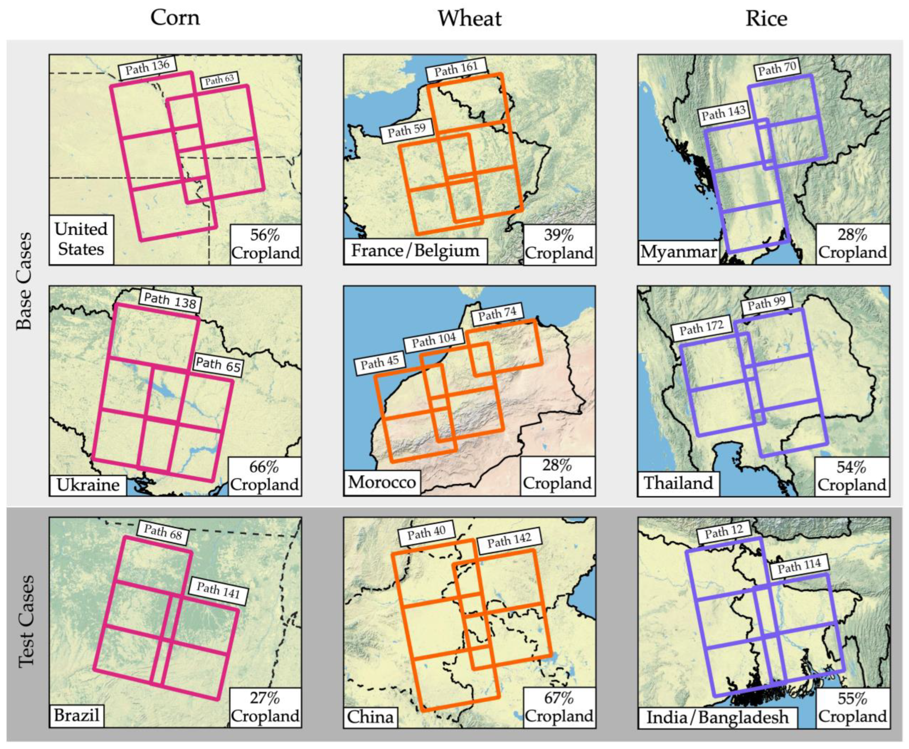
2.2.1. Areas of Interest
2.2.2. Data Preparation
2.2.3. Deriving Crop Type Thresholds
2.2.4. Performance Metrics
3. Results
4. Discussion
5. Conclusions
Author Contributions
Funding
Data Availability Statement
Acknowledgments
Conflicts of Interest
References
- Karthikeyan, L.; Chawla, I.; Mishra, A.K. A Review of Remote Sensing Applications in Agriculture for Food Security: Crop Growth and Yield, Irrigation, and Crop Losses. J. Hydrol. 2020, 586, 124905. [Google Scholar] [CrossRef]
- Economic Importance of Agriculture for Poverty Reduction; OECD Food, Agriculture and Fisheries Papers; OECD: Paris, France, 2010; Volume 23.
- Gillespie, S.; Van Den Bold, M. Agriculture, Food Systems, and Nutrition: Meeting the Challenge. Glob. Chall. 2017, 1, 1600002. [Google Scholar] [CrossRef] [PubMed]
- Robertson, G.P.; Swinton, S.M. Reconciling Agricultural Productivity and Environmental Integrity: A Grand Challenge for Agriculture. Front. Ecol. Environ. 2005, 3, 38–46. [Google Scholar] [CrossRef]
- Khanal, S.; Kc, K.; Fulton, J.P.; Shearer, S.; Ozkan, E. Remote Sensing in Agriculture—Accomplishments, Limitations, and Opportunities. Remote Sens. 2020, 12, 3783. [Google Scholar] [CrossRef]
- Benedict, T.D.; Brown, J.F.; Boyte, S.P.; Howard, D.M.; Fuchs, B.A.; Wardlow, B.D.; Tadesse, T.; Evenson, K.A. Exploring VIIRS Continuity with MODIS in an Expedited Capability for Monitoring Drought-Related Vegetation Conditions. Remote Sens. 2021, 13, 1210. [Google Scholar] [CrossRef]
- Ahmad, U.; Alvino, A.; Marino, S. A Review of Crop Water Stress Assessment Using Remote Sensing. Remote Sens. 2021, 13, 4155. [Google Scholar] [CrossRef]
- Hain, C.R.; Anderson, M.C. Estimating Morning Change in Land Surface Temperature from MODIS Day/Night Observations: Applications for Surface Energy Balance Modeling. Geophys. Res. Lett. 2017, 44, 9723–9733. [Google Scholar] [CrossRef]
- Abdullah, H.M.; Mohana, N.T.; Khan, B.M.; Ahmed, S.M.; Hossain, M.; Islam, K.S.; Redoy, M.H.; Ferdush, J.; Bhuiyan, M.A.H.B.; Hossain, M.M.; et al. Present and Future Scopes and Challenges of Plant Pest and Disease (P&D) Monitoring: Remote Sensing, Image Processing, and Artificial Intelligence Perspectives. Remote Sens. Appl. Soc. Environ. 2023, 32, 100996. [Google Scholar] [CrossRef]
- Debeurs, K.; Townsend, P. Estimating the Effect of Gypsy Moth Defoliation Using MODIS. Remote Sens. Environ. 2008, 112, 3983–3990. [Google Scholar] [CrossRef]
- Molthan, A.; Burks, J.; McGrath, K.; LaFontaine, F. Multi-Sensor Examination of Hail Damage Swaths for near Real-Time Applications and Assessment. J. Oper. Meteorol. 2013, 1, 144–156. [Google Scholar] [CrossRef]
- Bell, J.; Molthan, A. Evaluation of Approaches to Identifying Hail Damage to Crop Vegetation Using Satellite Imagery. J. Oper. Meteorol. 2016, 04, 142–159. [Google Scholar] [CrossRef]
- Flores-Anderson, A.; Herndon, K.; Cherrington, E.; Thapa, R. The SAR Handbook: Comprehensive Meth. for Forest Monitoring and Biomass Estimation; NASA: Washington, DC, USA, 2019; 307p. [Google Scholar]
- Prudente, V.H.R.; Martins, V.S.; Vieira, D.C.; Silva, N.R.D.F.E.; Adami, M.; Sanches, I.D. Limitations of Cloud Cover for Optical Remote Sensing of Agricultural Areas across South America. Remote Sens. Appl. Soc. Environ. 2020, 20, 100414. [Google Scholar] [CrossRef]
- McNairn, H.; Brisco, B. The Application of C-Band Polarimetric SAR for Agriculture: A Review. Can. J. Remote Sens. 2004, 30, 525–542. [Google Scholar] [CrossRef]
- Cable, J.; Kovacs, J.; Jiao, X.; Shang, J. Agricultural Monitoring in Northeastern Ontario, Canada, Using Multi-Temporal Polarimetric RADARSAT-2 Data. Remote Sens. 2014, 6, 2343–2371. [Google Scholar] [CrossRef]
- Forkuor, G.; Conrad, C.; Thiel, M.; Ullmann, T.; Zoungrana, E. Integration of Optical and Synthetic Aperture Radar Imagery for Improving Crop Mapping in Northwestern Benin, West Africa. Remote Sens. 2014, 6, 6472–6499. [Google Scholar] [CrossRef]
- Canisius, F.; Shang, J.; Liu, J.; Huang, X.; Ma, B.; Jiao, X.; Geng, X.; Kovacs, J.M.; Walters, D. Tracking Crop Phenological Development Using Multi-Temporal Polarimetric Radarsat-2 Data. Remote Sens. Environ. 2018, 210, 508–518. [Google Scholar] [CrossRef]
- Bell, J.R.; Gebremichael, E.; Molthan, A.L.; Schultz, L.A.; Meyer, F.J.; Hain, C.R.; Shrestha, S.; Payne, K.C. Complementing Optical Remote Sensing with Synthetic Aperture Radar Observations of Hail Damage Swaths to Agricultural Crops in the Central United States. J. Appl. Meteorol. Climatol. 2020, 59, 665–685. [Google Scholar] [CrossRef]
- Bell, J.R.; Bedka, K.M.; Schultz, C.J.; Molthan, A.L.; Bang, S.D.; Glisan, J.; Ford, T.; Lincoln, W.S.; Schultz, L.A.; Melancon, A.M.; et al. Satellite-Based Characterization of Convection and Impacts from the Catastrophic 10 August 2020 Midwest U.S. Derecho. Bull. Am. Meteorol. Soc. 2022, 103, E1172–E1196. [Google Scholar] [CrossRef]
- Khabbazan, S.; Vermunt, P.; Steele-Dunne, S.; Ratering Arntz, L.; Marinetti, C.; Van Der Valk, D.; Iannini, L.; Molijn, R.; Westerdijk, K.; Van Der Sande, C. Crop Monitoring Using Sentinel-1 Data: A Case Study from The Netherlands. Remote Sens. 2019, 11, 1887. [Google Scholar] [CrossRef]
- Nikaein, T.; Iannini, L.; Molijn, R.A.; Lopez-Dekker, P. On the Value of Sentinel-1 InSAR Coherence Time-Series for Vegetation Classification. Remote Sens. 2021, 13, 3300. [Google Scholar] [CrossRef]
- Nasirzadehdizaji, R.; Balik Sanli, F.; Abdikan, S.; Cakir, Z.; Sekertekin, A.; Ustuner, M. Sensitivity Analysis of Multi-Temporal Sentinel-1 SAR Parameters to Crop Height and Canopy Coverage. Appl. Sci. 2019, 9, 655. [Google Scholar] [CrossRef]
- Abdikan, S.; Sekertekin, A.; Ustunern, M.; Balik Sanli, F.; Nasirzadehdizaji, R. Backscatter Analysis Using Multi-Temporal Sentinel-1 Sar Data for Crop Growth of Maize in Konya Basin, Turkey. Int. Arch. Photogramm. Remote Sens. Spat. Inf. Sci. 2018, XLII–3, 9–13. [Google Scholar] [CrossRef]
- Dingle Robertson, L.; Davidson, A.M.; McNairn, H.; Hosseini, M.; Mitchell, S.; De Abelleyra, D.; Verón, S.; Le Maire, G.; Plannells, M.; Valero, S.; et al. C-Band Synthetic Aperture Radar (SAR) Imagery for the Classification of Diverse Cropping Systems. Int. J. Remote Sens. 2020, 41, 9628–9649. [Google Scholar] [CrossRef]
- Whelen, T.; Siqueira, P. Coefficient of Variation for Use in Crop Area Classification across Multiple Climates. Int. J. Appl. Earth Obs. Geoinf. 2018, 67, 114–122. [Google Scholar] [CrossRef]
- Kendall, M.G.; Stuart, A.; Ord, J.K. The Advanced Theory of Statistics. 1: Distribution Theory, 3rd ed.; Griffin: London, UK, 1969; ISBN 978-0-85264-141-5. [Google Scholar]
- Fawcett, T. An Introduction to ROC Analysis. Pattern Recognit. Lett. 2006, 27, 861–874. [Google Scholar] [CrossRef]
- Rose, S.; Kraatz, S.; Kellndorfer, J.; Cosh, M.H.; Torbick, N.; Huang, X.; Siqueira, P. Evaluating NISAR’s Cropland Mapping Algorithm over the Conterminous United States Using Sentinel-1 Data. Remote Sens. Environ. 2021, 260, 112472. [Google Scholar] [CrossRef]
- Youden, W.J. Index for Rating Diagnostic Tests. Cancer 1950, 3, 32–35. [Google Scholar] [CrossRef] [PubMed]
- Habibzadeh, F.; Habibzadeh, P.; Yadollahie, M. On Determining the Most Appropriate Test Cut-off Value: The Case of Tests with Continuous Results. Biochem. Med. 2016, 26, 297–307. [Google Scholar] [CrossRef]
- Kraatz, S.; Lamb, B.T.; Hively, W.D.; Jennewein, J.S.; Gao, F.; Cosh, M.H.; Siqueira, P. Comparing NISAR (Using Sentinel-1), USDA/NASS CDL, and Ground Truth Crop/Non-Crop Areas in an Urban Agricultural Region. Sensors 2023, 23, 8595. [Google Scholar] [CrossRef]
- Boryan, C.; Yang, Z.; Mueller, R.; Craig, M. Monitoring US Agriculture: The US Department of Agriculture, National Agricultural Statistics Service, Cropland Data Layer Program. Geocarto Int. 2011, 26, 341–358. [Google Scholar] [CrossRef]
- NASA-ISRO SAR (NISAR) Mission Science Users’ Handbook, NASA, 9 April 2018, Version 1. Available online: https://nisar.jpl.nasa.gov/system/documents/files/26_NISAR_FINAL_9-6-19.pdf (accessed on 31 July 2024).
- Kraatz, S.; Siqueira, P.; Kellndorfer, J.; Torbick, N.; Huang, X.; Cosh, M. Evaluating the Robustness of NISAR’s Cropland Product to Time of Observation, Observing Mode, and Dithering. Earth Space Sci. 2022, 9, e2022EA002366. [Google Scholar] [CrossRef]
- Small, D. Flattening Gamma: Radiometric Terrain Correction for SAR Imagery. IEEE Trans. Geosci. Remote Sens. 2011, 49, 3081–3093. [Google Scholar] [CrossRef]
- Hogenson, K.; Arko, S.A.; Buechler, B.; Hogenson, R.; Herrmann, J.; Geiger, A. Hybrid Pluggable Processing Pipeline (HyP3): A cloud-based infrastructure for generic processing of SAR data. In Proceedings of the Agu Fall Meeting Abstracts, San Francisco, CA, USA, 12–16 December 2016; Volume 2016, p. IN21B-1740. [Google Scholar]
- Meyer, F.J.; Schultz, L.A.; Osmanoglu, B.; Kennedy, J.H.; Jo, M.; Thapa, R.B.; Bell, J.R.; Pradhan, S.; Shrestha, M.; Smale, J.; et al. HydroSAR: A Cloud-Based Service for the Monitoring of Inundation Events in the Hindu Kush Himalaya. Remote Sens. 2024, 16, 3244. [Google Scholar] [CrossRef]
- Loew, A.; Mauser, W. Generation of Geometrically and Radiometrically Terrain Corrected SAR Image Products. Remote Sens. Environ. 2007, 106, 337–349. [Google Scholar] [CrossRef]
- Vreugdenhil, M.; Wagner, W.; Bauer-Marschallinger, B.; Pfeil, I.; Teubner, I.; Rüdiger, C.; Strauss, P. Sensitivity of Sentinel-1 Backscatter to Vegetation Dynamics: An Austrian Case Study. Remote Sens. 2018, 10, 1396. [Google Scholar] [CrossRef]
- Wang, J.; Dai, Q.; Shang, J.; Jin, X.; Sun, Q.; Zhou, G.; Dai, Q. Field-Scale Rice Yield Estimation Using Sentinel-1A Synthetic Aperture Radar (SAR) Data in Coastal Saline Region of Jiangsu Province, China. Remote Sens. 2019, 11, 2274. [Google Scholar] [CrossRef]
- Huang, X.; Reba, M.; Coffin, A.; Runkle, B.R.K.; Huang, Y.; Chapman, B.; Ziniti, B.; Skakun, S.; Kraatz, S.; Siqueira, P.; et al. Cropland Mapping with L-Band UAVSAR and Development of NISAR Products. Remote Sens. Environ. 2021, 253, 112180. [Google Scholar] [CrossRef]
- McNairn, H.; Shang, J.; Jiao, X.; Champagne, C. The Contribution of ALOS PALSAR Multipolarization and Polarimetric Data to Crop Classification. IEEE Trans. Geosci. Remote Sens. 2009, 47, 3981–3992. [Google Scholar] [CrossRef]
- Buchhorn, M.; Smets, B.; Bertels, L.; Roo, B.D.; Lesiv, M.; Tsendbazar, N.-E.; Herold, M.; Fritz, S. Copernicus Global Land Service: Land Cover 2018 (Raster 100 m), Global, Yearly–Version 3, Epoch 2018, European Union’s Copernicus Land Monitoring Service Information. Available online: https://land.copernicus.eu/en/products/global-dynamic-land-cover/copernicus-global-land-service-land-cover-100m-collection-3-epoch-2018-globe (accessed on 21 August 2024).
- Buchhorn, M.; Smets, B.; Bertels, L.; Roo, B.D.; Lesiv, M.; Tsendbazar, N.-E.; Herold, M.; Fritz, S. Copernicus Global Land Service: Land Cover 2019 (Raster 100 m), Global, Yearly–Version 3, Epoch 2019, European Union’s Copernicus Land Monitoring Service Information. Available online: https://land.copernicus.eu/en/products/global-dynamic-land-cover/copernicus-global-land-service-land-cover-100m-collection-3-epoch-2019-globe (accessed on 24 August 2024).
- Zanaga, D.; Van De Kerchove, R.; De Keersmaecker, W.; Souverijns, N.; Brockmann, C.; Quast, R.; Wevers, J.; Grosu, A.; Paccini, A.; Vergnaud, S.; et al. ESA WorldCover 10 m 2020 v100. 2021. Available online: https://zenodo.org/records/5571936 (accessed on 27 August 2024).
- Zanaga, D.; Van De Kerchove, R.; Daems, D.; De Keersmaecker, W.; Brockmann, C.; Kirches, G.; Wevers, J.; Cartus, O.; Santoro, M.; Fritz, S.; et al. ESA WorldCover 10 m 2021 v200. 2022. Available online: https://zenodo.org/records/7254221 (accessed on 30 August 2024).
- Food and Agriculture Organization of the United States (FAO). Agricultural Production Statistics 2020–2021. 2021. Available online: https://openknowledge.fao.org/server/api/core/bitstreams/58971ed8-c831-4ee6-ab0a-e47ea66a7e6a/content (accessed on 20 September 2024).
- Bullock, D.G. Crop Rotation. Crit. Rev. Plant Sci. 1992, 11, 309–326. [Google Scholar] [CrossRef]
- Sindelar, A.J.; Schmer, M.R.; Jin, V.L.; Wienhold, B.J.; Varvel, G.E. Long-Term Corn and Soybean Response to Crop Rotation and Tillage. Agron. J. 2015, 107, 2241–2252. [Google Scholar] [CrossRef]
- Rotundo, J.L.; Rech, R.; Cardoso, M.M.; Fang, Y.; Tang, T.; Olson, N.; Pyrik, B.; Conrad, G.; Borras, L.; Mihura, E.; et al. Development of a Decision-Making Application for Optimum Soybean and Maize Fertilization Strategies in Mato Grosso. Comput. Electron. Agric. 2022, 193, 106659. [Google Scholar] [CrossRef]
- Kussul, N.; Deininger, K.; Lavreniuk, M.; Ali, D.A.; Nivievskyi, O. Using Machine Learning to Assess Yield Impacts of Crop Rotation: Combining Satellite and Statistical Data for Ukraine; World Bank: Washington, DC, USA, 2020. [Google Scholar]
- USDA FAS Crop Production Maps, USDA. Available online: https://ipad.fas.usda.gov/ogamaps/cropproductionmaps.aspx (accessed on 31 July 2024).
- Meyer, F.J.; Rosen, P.A.; Flores, A.; Anderson, E.R.; Cherrington, E.A. Making Sar Accessible: Education & Training in Preparation for Nisar. In Proceedings of the 2021 IEEE International Geoscience and Remote Sensing Symposium IGARSS, Brussels, Belgium, 11 July 2021; pp. 6–9. [Google Scholar]
- Cigna, F.; Bateson, L.B.; Jordan, C.J.; Dashwood, C. Simulating SAR Geometric Distortions and Predicting Persistent Scatterer Densities for ERS-1/2 and ENVISAT C-Band SAR and InSAR Applications: Nationwide Feasibility Assessment to Monitor the Landmass of Great Britain with SAR Imagery. Remote Sens. Environ. 2014, 152, 441–466. [Google Scholar] [CrossRef]
- Tupin, F.; Houshmand, B.; Datcu, M. Road Detection in Dense Urban Areas Using SAR Imagery and the Usefulness of Multiple Views. IEEE Trans. Geosci. Remote Sens. 2002, 40, 2405–2414. [Google Scholar] [CrossRef]
- Reschke, J.; Bartsch, A.; Schlaffer, S.; Schepaschenko, D. Capability of C-Band SAR for Operational Wetland Monitoring at High Latitudes. Remote Sens. 2012, 4, 2923–2943. [Google Scholar] [CrossRef]
- Bartsch, A.; Trofaier, A.M.; Hayman, G.; Sabel, D.; Schlaffer, S.; Clark, D.B.; Blyth, E. Detection of Open Water Dynamics with ENVISAT ASAR in Support of Land Surface Modelling at High Latitudes. Biogeosciences 2012, 9, 703–714. [Google Scholar] [CrossRef]
- Lark, T.J.; Mueller, R.M.; Johnson, D.M.; Gibbs, H.K. Measuring Land-Use and Land-Cover Change Using the U.S. Department of Agriculture’s Cropland Data Layer: Cautions and Recommendations. Int. J. Appl. Earth Obs. Geoinf. 2017, 62, 224–235. [Google Scholar] [CrossRef]
- Wang, Y.; Hess, L.L.; Filoso, S.; Melack, J.M. Canopy Penetration Studies: Modeled Radar Backscatter from Amazon Floodplain Forests at C-, L-, and P-Band. In Proceedings of the IGARSS ’94—1994 IEEE International Geoscience and Remote Sensing Symposium, Pasadena, CA, USA, 8–12 August 1994; Volume 2, pp. 1060–1062. [Google Scholar] [CrossRef]
- McNairn, H.; Boisvert, J.B.; Major, D.J.; Gwyn, Q.H.J.; Brown, R.J.; Smith, A.M. Identification of Agricultural Tillage Practices from C-Band Radar Backscatter. Can. J. Remote Sens. 1996, 22, 154–162. [Google Scholar] [CrossRef]
- Zheng, B.; Campbell, J.B.; Serbin, G.; Galbraith, J.M. Remote Sensing of Crop Residue and Tillage Practices: Present Capabilities and Future Prospects. Soil Tillage Res. 2014, 138, 26–34. [Google Scholar] [CrossRef]
- Bazzi, H.; Baghdadi, N.; Charron, F.; Zribi, M. Comparative Analysis of the Sensitivity of SAR Data in C and L Bands for the Detection of Irrigation Events. Remote Sens. 2022, 14, 2312. [Google Scholar] [CrossRef]
- Ranjbar, S.; Akhoondzadeh, M.; Brisco, B.; Amani, M.; Hosseini, M. Soil Moisture Change Monitoring from C and L-Band SAR Interferometric Phase Observations. IEEE J. Sel. Top. Appl. Earth Obs. Remote Sens. 2021, 14, 7179–7197. [Google Scholar] [CrossRef]
- Ajadi, O.A.; Barr, J.; Liang, S.-Z.; Ferreira, R.; Kumpatla, S.P.; Patel, R.; Swatantran, A. Large-Scale Crop Type and Crop Area Mapping across Brazil Using Synthetic Aperture Radar and Optical Imagery. Int. J. Appl. Earth Obs. Geoinf. 2021, 97, 102294. [Google Scholar] [CrossRef]
- Wang, X.; Zhang, X. A Regional Comparative Study on the Mismatch between Population Urbanization and Land Urbanization in China. PLoS ONE 2023, 18, e0287366. [Google Scholar] [CrossRef] [PubMed]
- Shen, R.; Pan, B.; Peng, Q.; Dong, J.; Chen, X.; Zhang, X.; Ye, T.; Huang, J.; Yuan, W. High-Resolution Distribution Maps of Single-Season Rice in China from 2017 to 2022. Earth Syst. Sci. Data 2023, 15, 3203–3222. [Google Scholar] [CrossRef]
- Moumni, A.; Lahrouni, A. Machine Learning-Based Classification for Crop-Type Mapping Using the Fusion of High-Resolution Satellite Imagery in a Semiarid Area. Scientifica 2021, 2021, 1–20. [Google Scholar] [CrossRef]
- Tufail, R.; Ahmad, A.; Javed, M.A.; Ahmad, S.R. A Machine Learning Approach for Accurate Crop Type Mapping Using Combined SAR and Optical Time Series Data. Adv. Space Res. 2022, 69, 331–346. [Google Scholar] [CrossRef]
- Kraatz, S.; Rose, S.; Cosh, M.H.; Torbick, N.; Huang, X.; Siqueira, P. Performance Evaluation of UAVSAR and Simulated NISAR Data for Crop/Noncrop Classification Over Stoneville, MS. Earth Space Sci. 2021, 8, e2020EA001363. [Google Scholar] [CrossRef]
- El Hajj, M.; Baghdadi, N.; Bazzi, H.; Zribi, M. Penetration Analysis of SAR Signals in the C and L Bands for Wheat, Maize, and Grasslands. Remote Sens. 2018, 11, 31. [Google Scholar] [CrossRef]
- Rosenqvist, A.; Killough, B. A Layman’s Interpretation Guide to L-Band and C-Band Synthetic Aperture Radar Data; Committee on Earth Observation Satellites (CEOS): Washington, DC, USA, 2023. [Google Scholar]


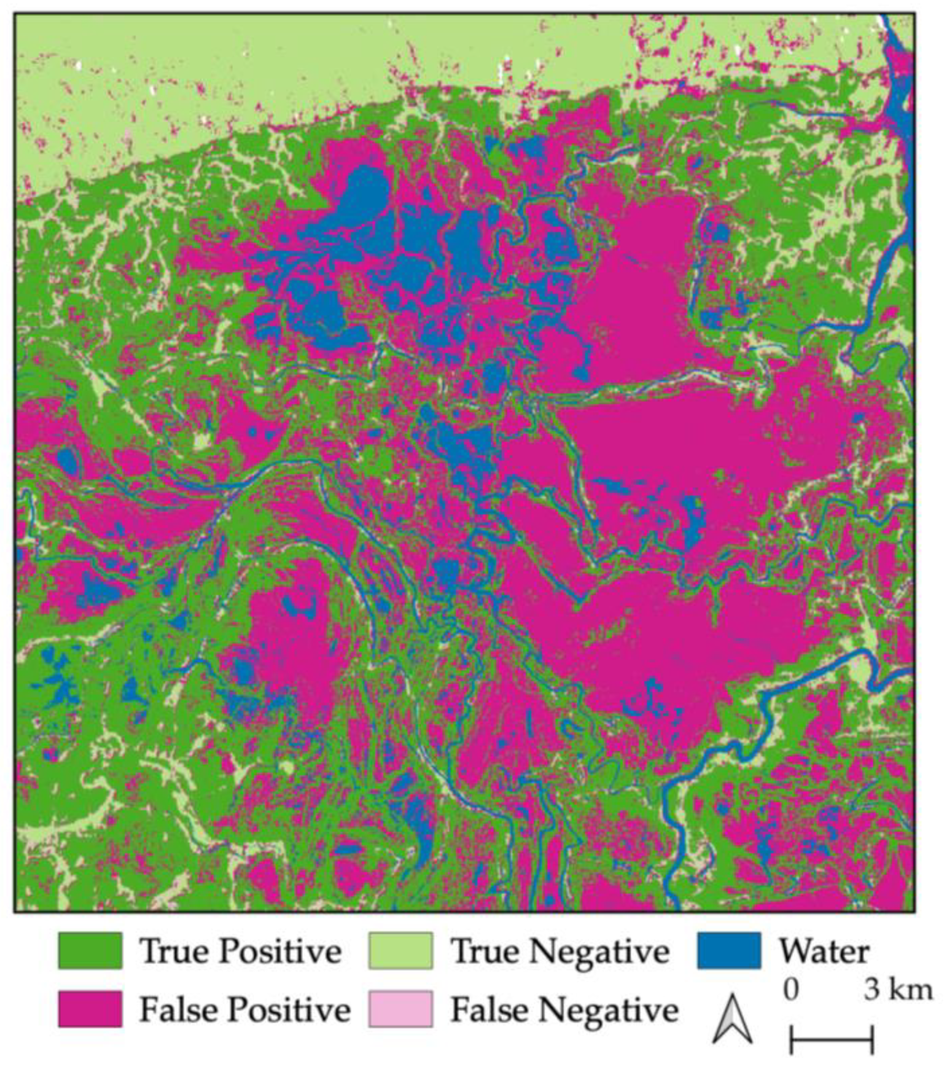
| Positive Classification | Negative Classification |
|---|---|
| √ True Positive: Pixel classified as “crop” by CV threshold, and it is cropland in the reference layer. | √ True Negative: Pixel classified as “non-crop” by CV threshold, and it is non-cropland in the reference layer. |
| × False Positive: Pixel classified as “crop” by CV threshold, but it is not cropland in the reference layer. | × False Negative: Pixel classified as “non-crop” by CV threshold, but it is not cropland in the reference layer. |
| AOI | Year | Optimal CV Threshold | Accuracy | Sensitivity | Specificity |
|---|---|---|---|---|---|
| Ukraine | 2018 | 0.56 | 80.49 | 78.71 | 85.88 |
| 2019 | 0.50 | 81.40 | 80.09 | 85.33 | |
| 2020 | 0.53 | 86.45 | 88.27 | 82.26 | |
| 2021 | 0.57 | 86.74 | 88.44 | 83.10 | |
| 2022 | 0.59 | 87.99 | 87.93 | 88.11 | |
| Midwest United States | 2018 | 0.50 | 76.39 | 76.75 | 75.63 |
| 2019 | 0.48 | 77.53 | 75.13 | 82.65 | |
| 2020 | 0.51 | 82.37 | 83.53 | 90.76 | |
| 2021 | 0.55 | 83.83 | 84.40 | 83.10 | |
| 2022 | 0.55 | 80.02 | 86.95 | 71.11 | |
| Morocco | 2018 | 0.33 | 76.71 | 66.50 | 83.13 |
| 2019 | 0.28 | 74.17 | 60.13 | 83.02 | |
| 2020 | 0.28 | 77.06 | 67.32 | 80.97 | |
| 2021 | 0.36 | 82.82 | 71.38 | 87.83 | |
| 2022 | 0.28 | 78.21 | 73.85 | 80.12 | |
| France/Belgium | 2018 | 0.33 | 82.16 | 78.58 | 85.71 |
| 2019 | 0.29 | 82.30 | 79.70 | 84.87 | |
| 2020 | 0.33 | 88.03 | 88.56 | 87.68 | |
| 2021 | 0.31 | 89.23 | 89.23 | 89.02 | |
| 2022 | 0.32 | 89.47 | 89.47 | 89.02 | |
| Thailand | 2018 | 0.21 | 81.74 | 80.91 | 83.52 |
| 2019 | 0.22 | 83.53 | 83.93 | 82.67 | |
| 2020 | 0.29 | 86.88 | 88.55 | 84.63 | |
| 2021 | 0.25 | 85.97 | 88.02 | 83.53 | |
| 2022 | 0.24 | 84.76 | 86.78 | 82.39 | |
| Myanmar | 2018 | 0.25 | 80.38 | 76.67 | 83.47 |
| 2019 | 0.26 | 80.69 | 78.47 | 82.54 | |
| 2020 | 0.30 | 82.50 | 85.74 | 80.83 | |
| 2021 | 0.29 | 83.87 | 87.62 | 81.91 | |
| 2022 | 0.27 | 84.23 | 85.02 | 83.82 |
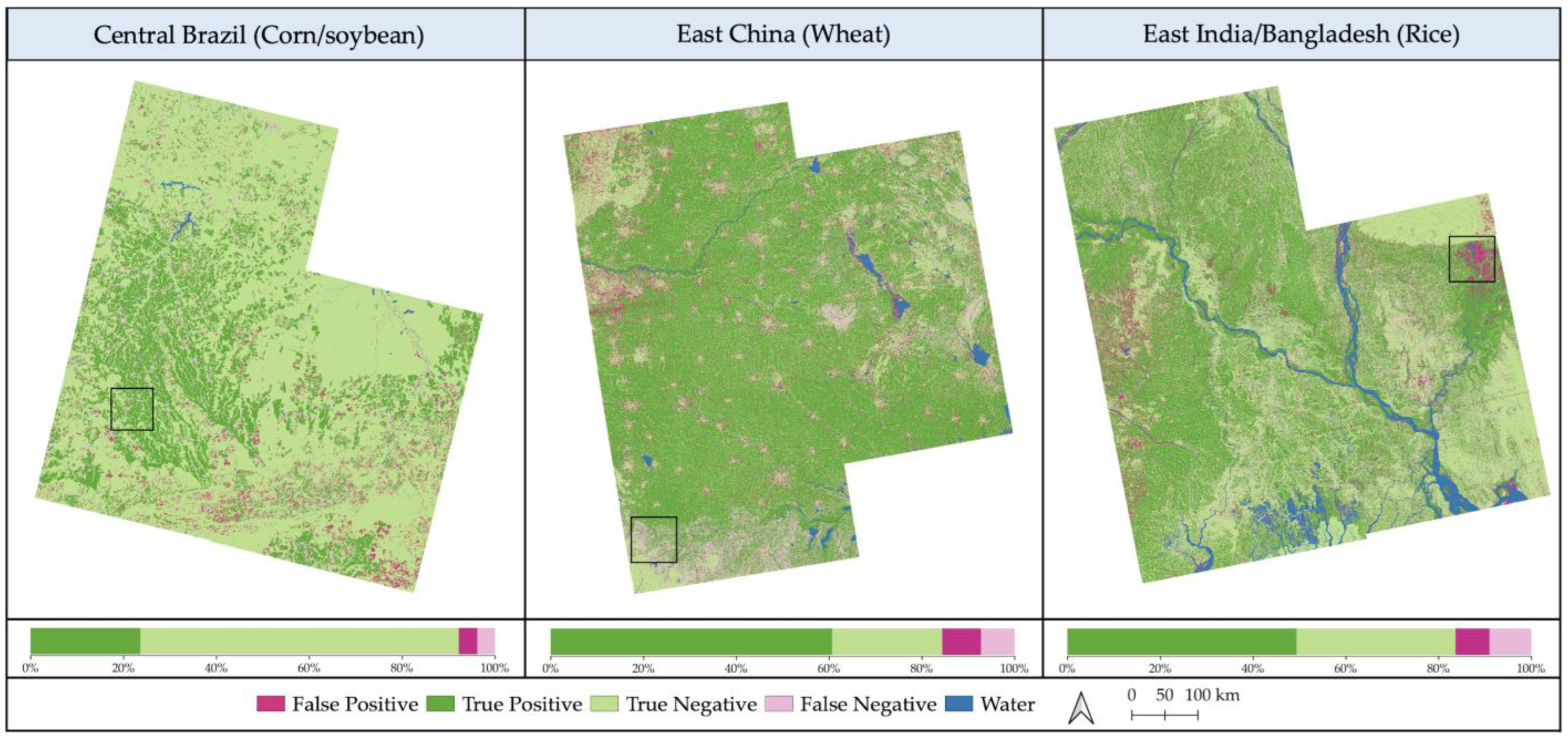
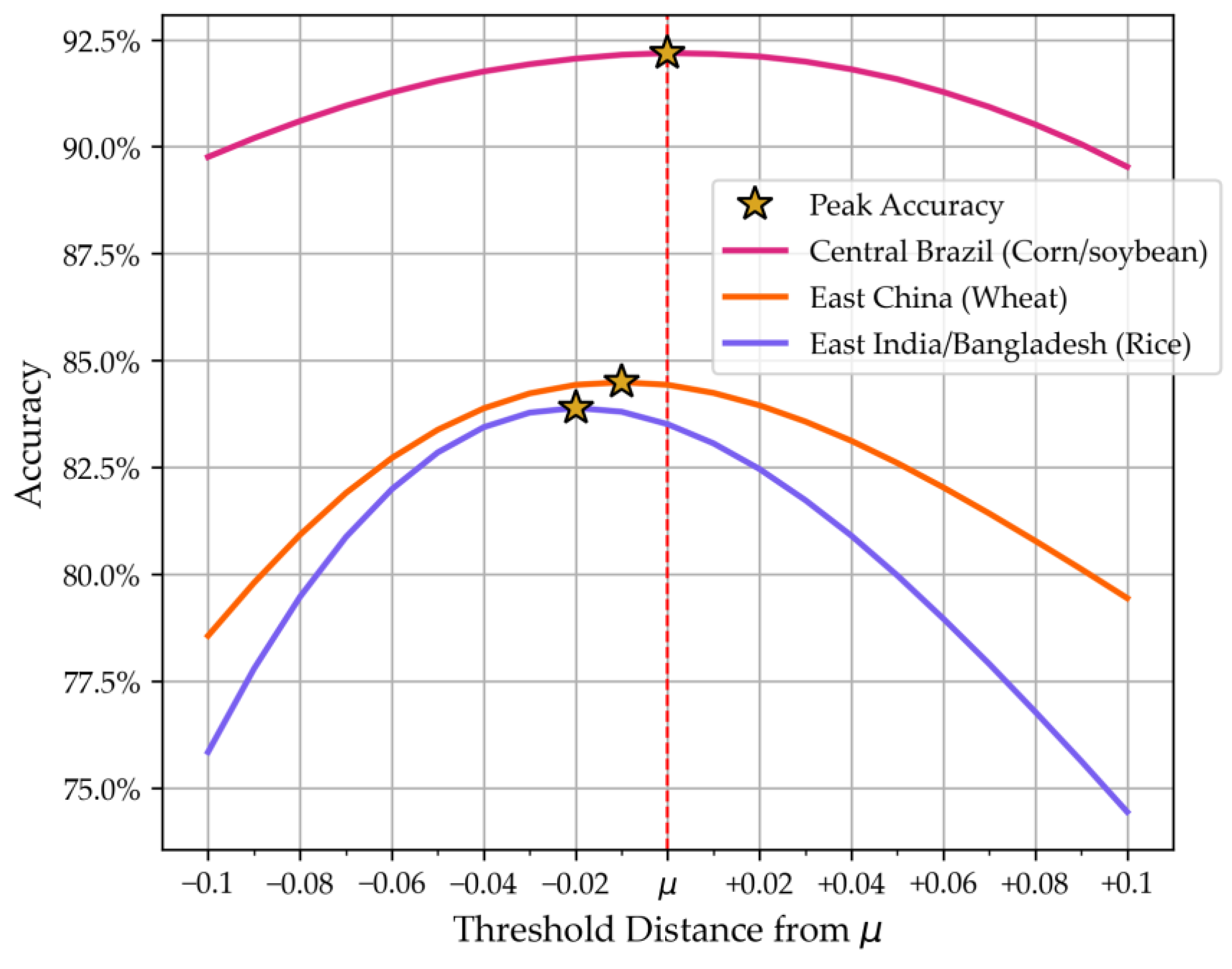
| Test Case AOI | Crop Type Threshold | Accuracy | Sensitivity | Specificity |
|---|---|---|---|---|
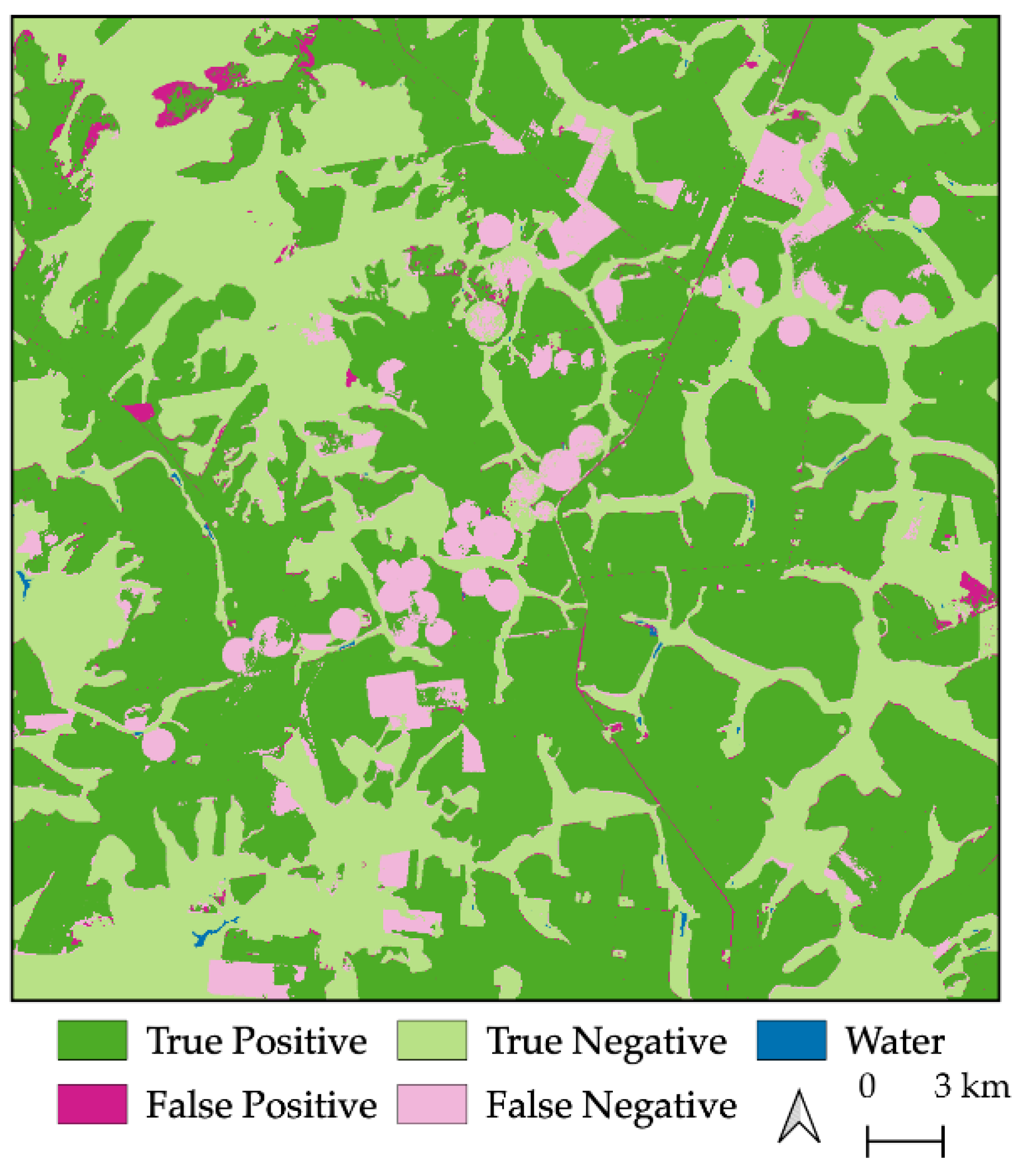
| Central Brazil (Corn/soybean) | 0.53 | 92.23 | 86.16 | 94.52 |
| East China (Wheat) | 0.31 | 84.43 | 89.36 | 73.99 |
| East India/Bangladesh (Rice) | 0.26 | 83.67 | 84.54 | 82.44 |
| Crop Type | Recommended Threshold |
|---|---|
| Corn/soybean | 0.53 ± 0.02 |
| Wheat | 0.31 ± 0.02 |
| Rice | 0.26 ± 0.02 |
Disclaimer/Publisher’s Note: The statements, opinions and data contained in all publications are solely those of the individual author(s) and contributor(s) and not of MDPI and/or the editor(s). MDPI and/or the editor(s) disclaim responsibility for any injury to people or property resulting from any ideas, methods, instructions or products referred to in the content. |
© 2025 by the authors. Licensee MDPI, Basel, Switzerland. This article is an open access article distributed under the terms and conditions of the Creative Commons Attribution (CC BY) license (https://creativecommons.org/licenses/by/4.0/).
Share and Cite
Sharp, K.G.; Bell, J.R.; Pankratz, H.G.; Schultz, L.A.; Lucey, R.; Meyer, F.J.; Molthan, A.L. Modifying NISAR’s Cropland Area Algorithm to Map Cropland Extent Globally. Remote Sens. 2025, 17, 1094. https://doi.org/10.3390/rs17061094
Sharp KG, Bell JR, Pankratz HG, Schultz LA, Lucey R, Meyer FJ, Molthan AL. Modifying NISAR’s Cropland Area Algorithm to Map Cropland Extent Globally. Remote Sensing. 2025; 17(6):1094. https://doi.org/10.3390/rs17061094
Chicago/Turabian StyleSharp, Kaylee G., Jordan R. Bell, Hannah G. Pankratz, Lori A. Schultz, Ronan Lucey, Franz J. Meyer, and Andrew L. Molthan. 2025. "Modifying NISAR’s Cropland Area Algorithm to Map Cropland Extent Globally" Remote Sensing 17, no. 6: 1094. https://doi.org/10.3390/rs17061094
APA StyleSharp, K. G., Bell, J. R., Pankratz, H. G., Schultz, L. A., Lucey, R., Meyer, F. J., & Molthan, A. L. (2025). Modifying NISAR’s Cropland Area Algorithm to Map Cropland Extent Globally. Remote Sensing, 17(6), 1094. https://doi.org/10.3390/rs17061094