

FTIR-SpectralGAN: A Spectral Data Augmentation Generative Adversarial Network for Aero-Engine Hot Jet FTIR Spectral Classification

Abstract
1. Introduction
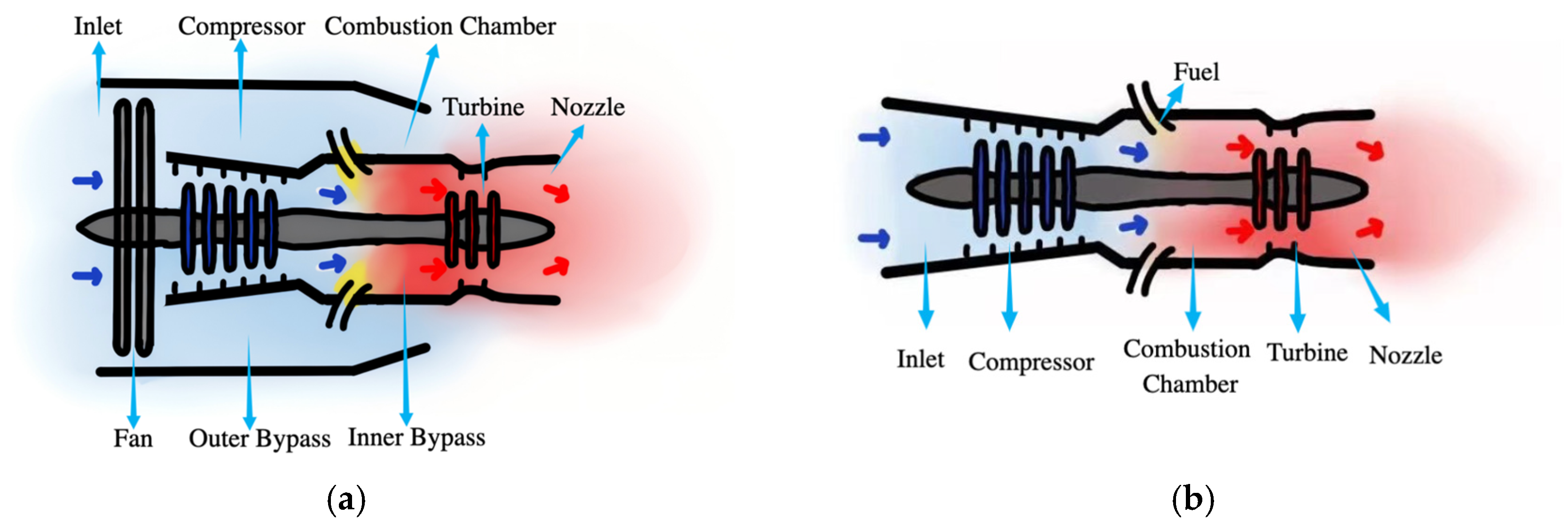
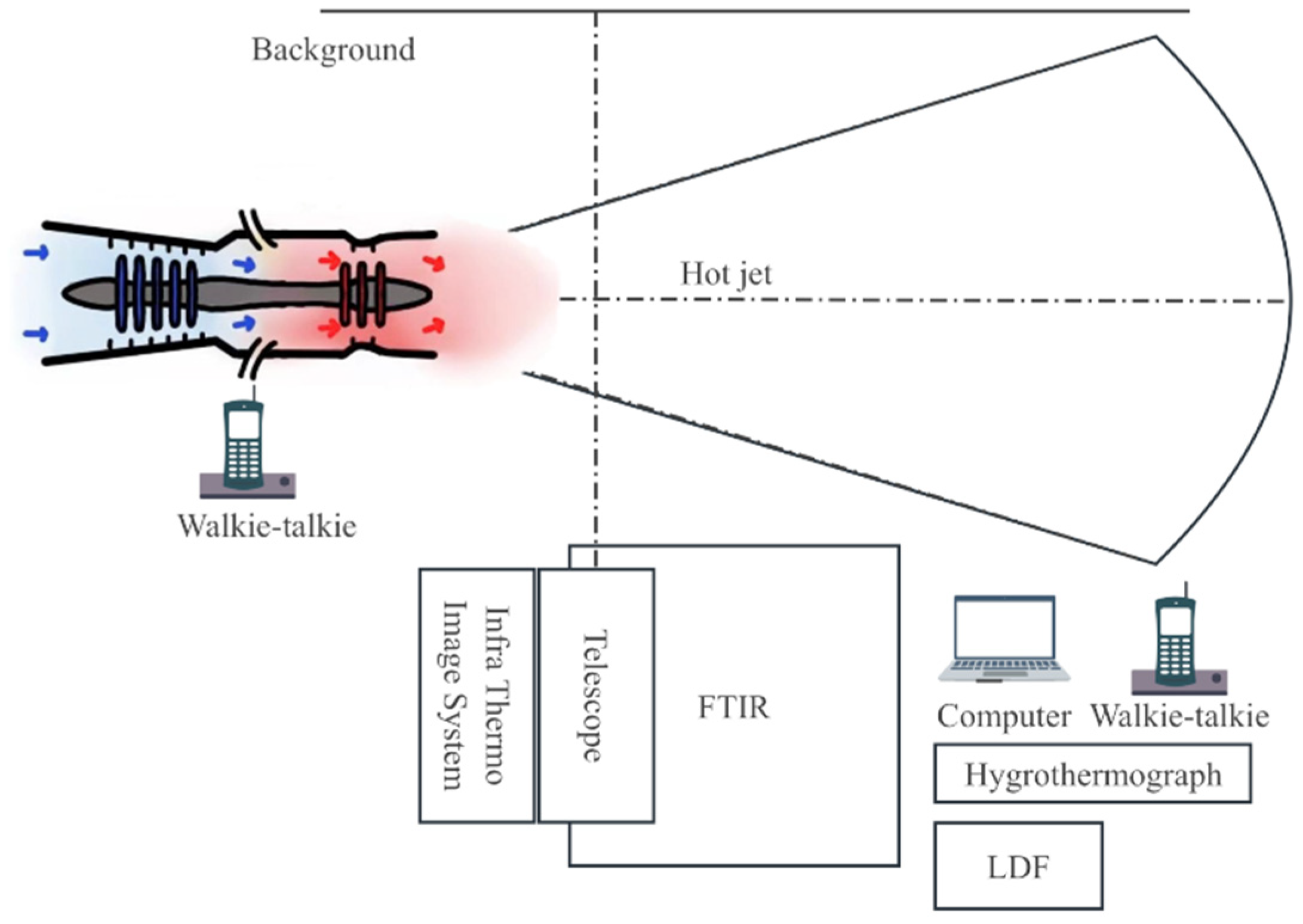
- The study employs outfield experiments to conduct infrared spectroscopy measurements on the hot jets of six types of aero-engines. Given that materials possess selective absorption capabilities for infrared radiation, utilizing the infrared spectra of hot jets as data support for the classification of aero-engines is scientifically sound and reliable.
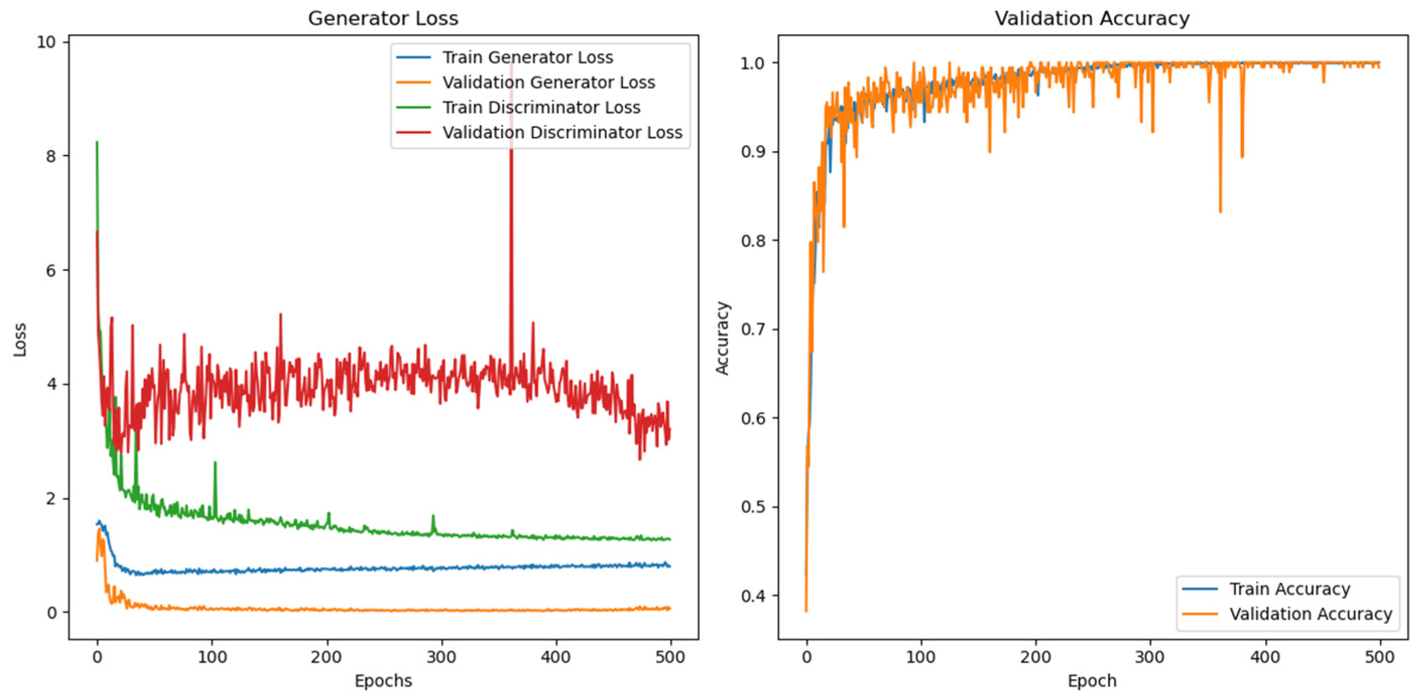
- This research utilizes an improved FTIR-SpectralGAN network based on DCGAN to address overfitting issues caused by limited sample sizes in infrared spectrum classification. Specifically, FTIR-SpectralGAN adopts 1D processing tailored to the data format of infrared spectra, diverging from traditional 2D operations. In terms of training strategy, an unbalanced approach is implemented where the generator undergoes initial training. Following each update of the discriminator, the generator parameters are optimized five times, effectively mitigating mode oscillation during adversarial training. Additionally, a weighted mixed loss strategy is employed with greater emphasis placed on classification loss to enhance the discriminator’s classification capability. Label smoothing regularization is also adopted, setting the label of real samples to 0.9 and combining it with a soft label strategy for generated samples set at 0.1.
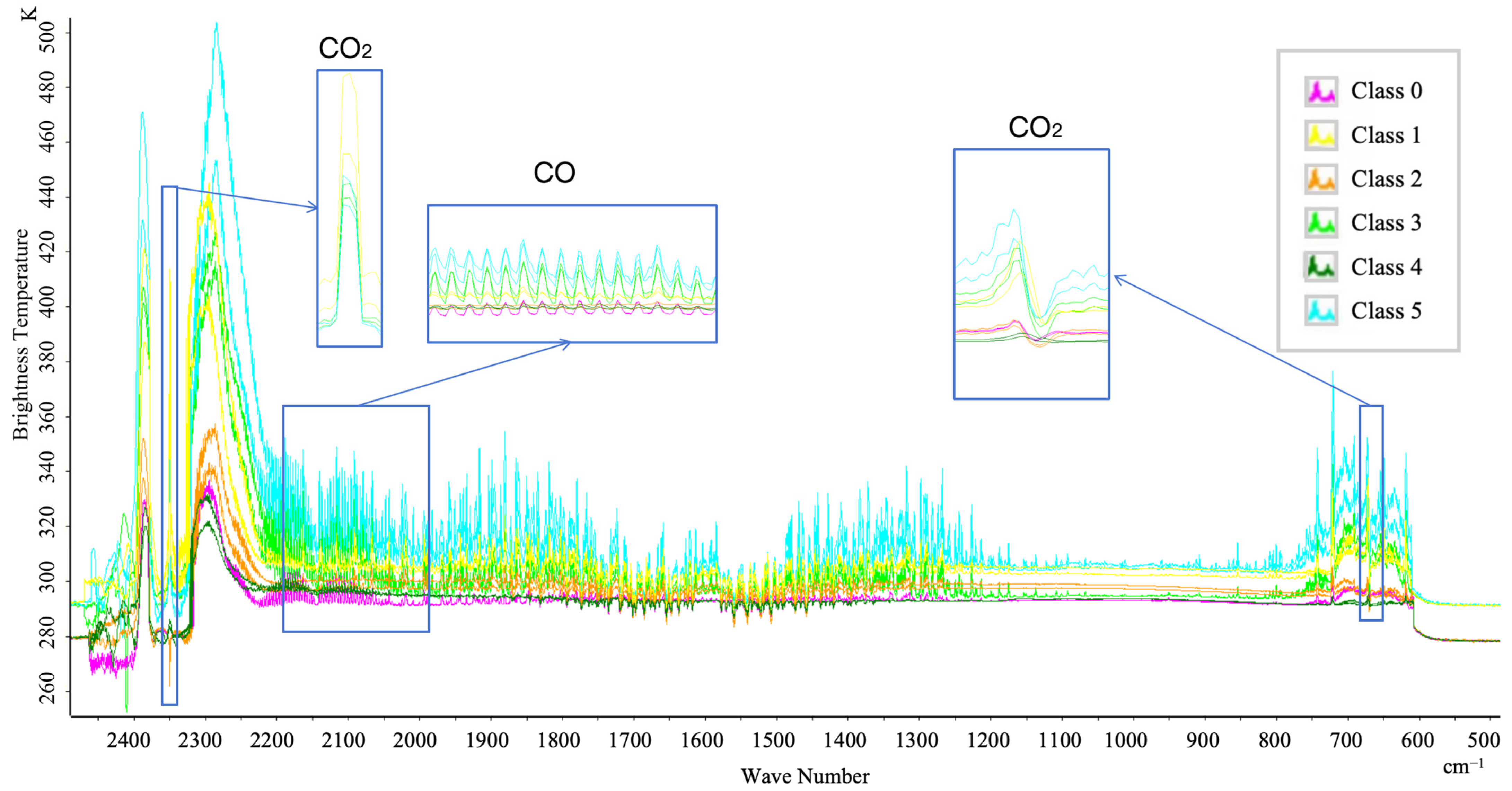
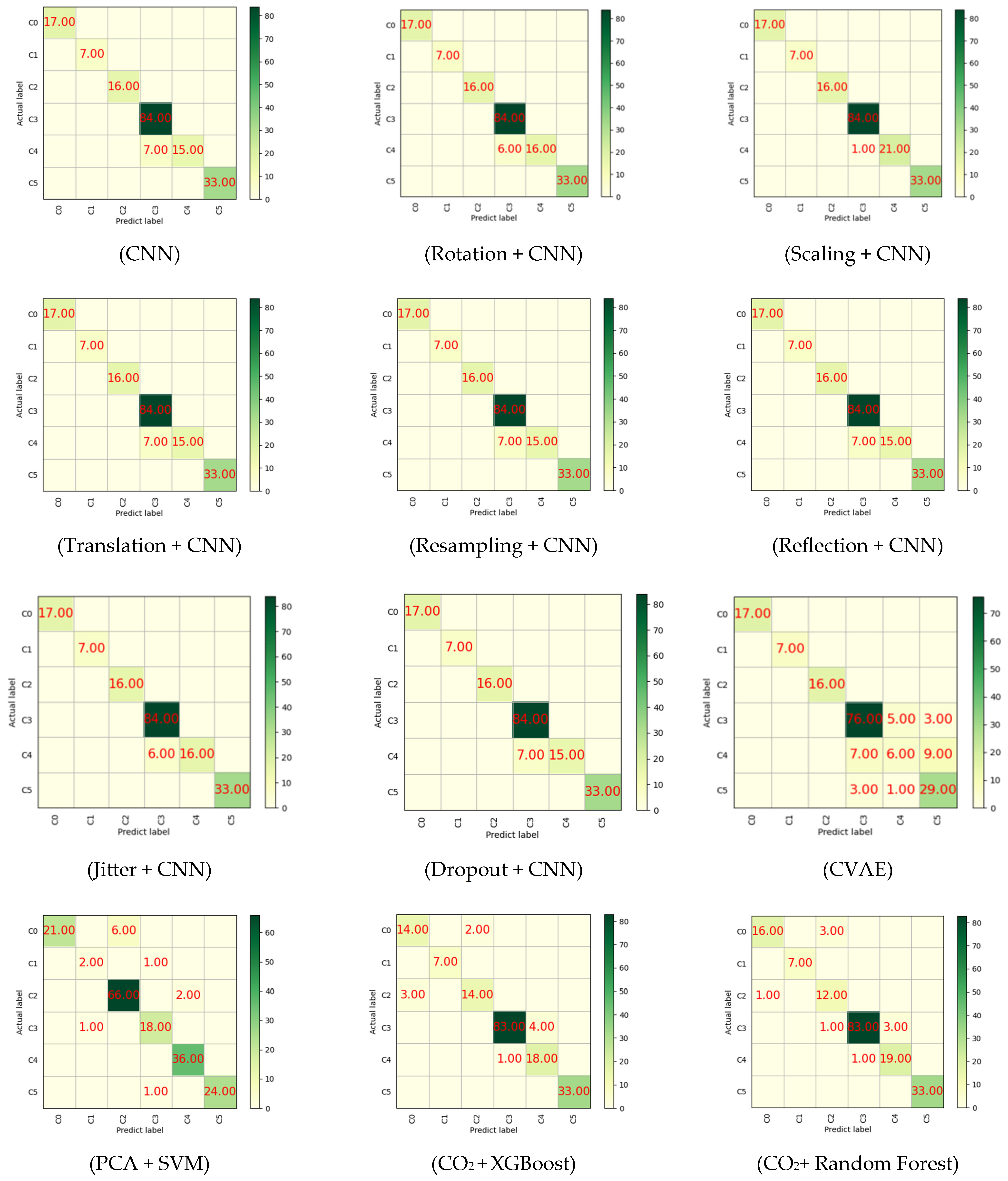
- The paper conducts experiments using both classic data augmentation methods (such as rotation, scaling, translation, resampling, mirroring, jittering, and discarding) and the deep learning-based data augmentation method CVAE, comparing their performance on spectral datasets. In addition, classical spectral feature extraction methods, including one-dimensional convolutional neural networks (1DCNNs), principal component analysis (PCA), and CO2 feature vectors, were incorporated into the comparison experiment alongside the classifier.
2. Material and Methods
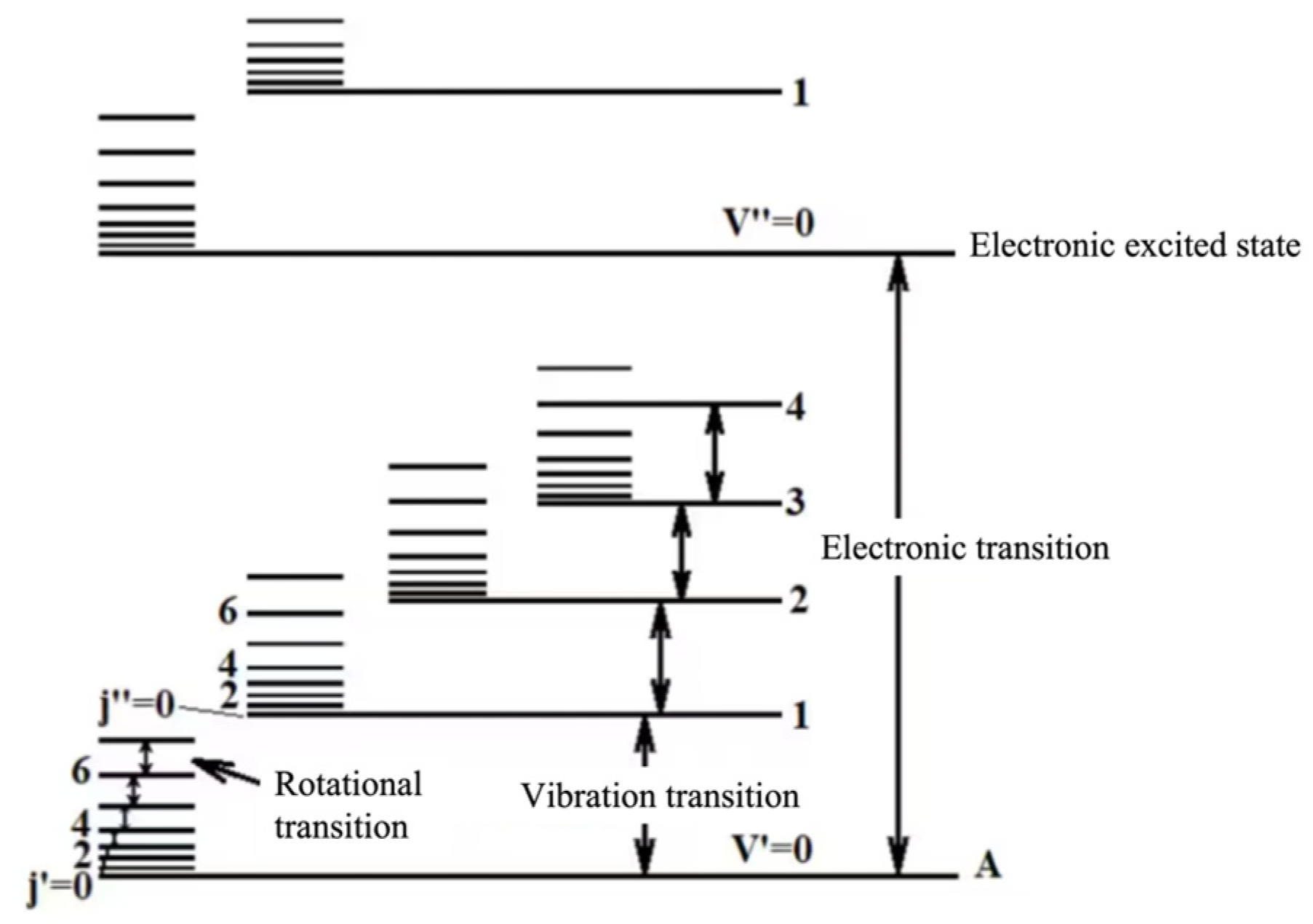
2.1. The Principle of Aero-Engine Hot Jet Spectral Classification
2.2. Spectral Dataset
2.2.1. Experimental Design for Aero-Engine Spectral Measurement
2.2.2. Spectral Dataset Production
2.3. The Spectral Classification Network Structure Design Method
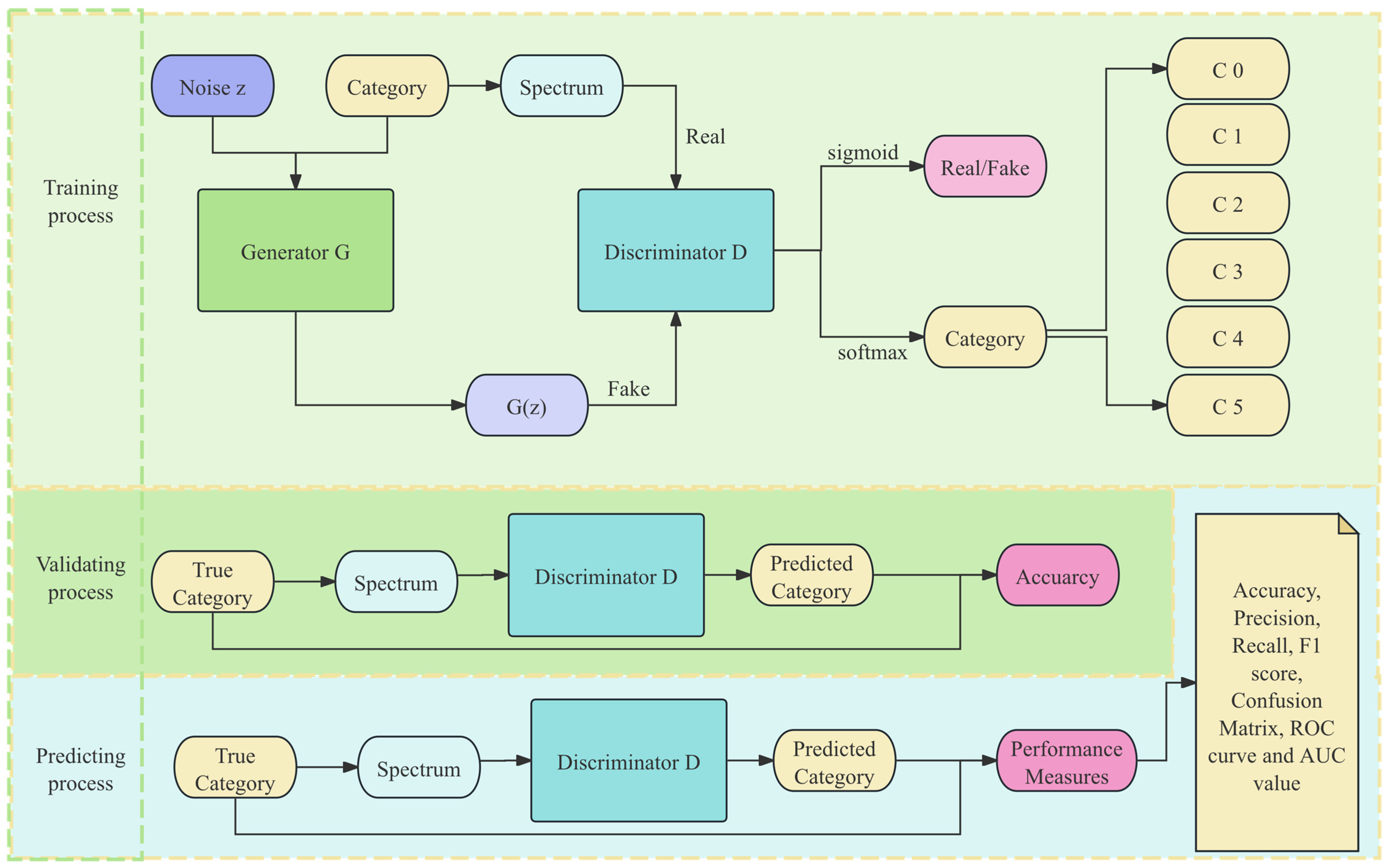
2.3.1. Overall Network Design
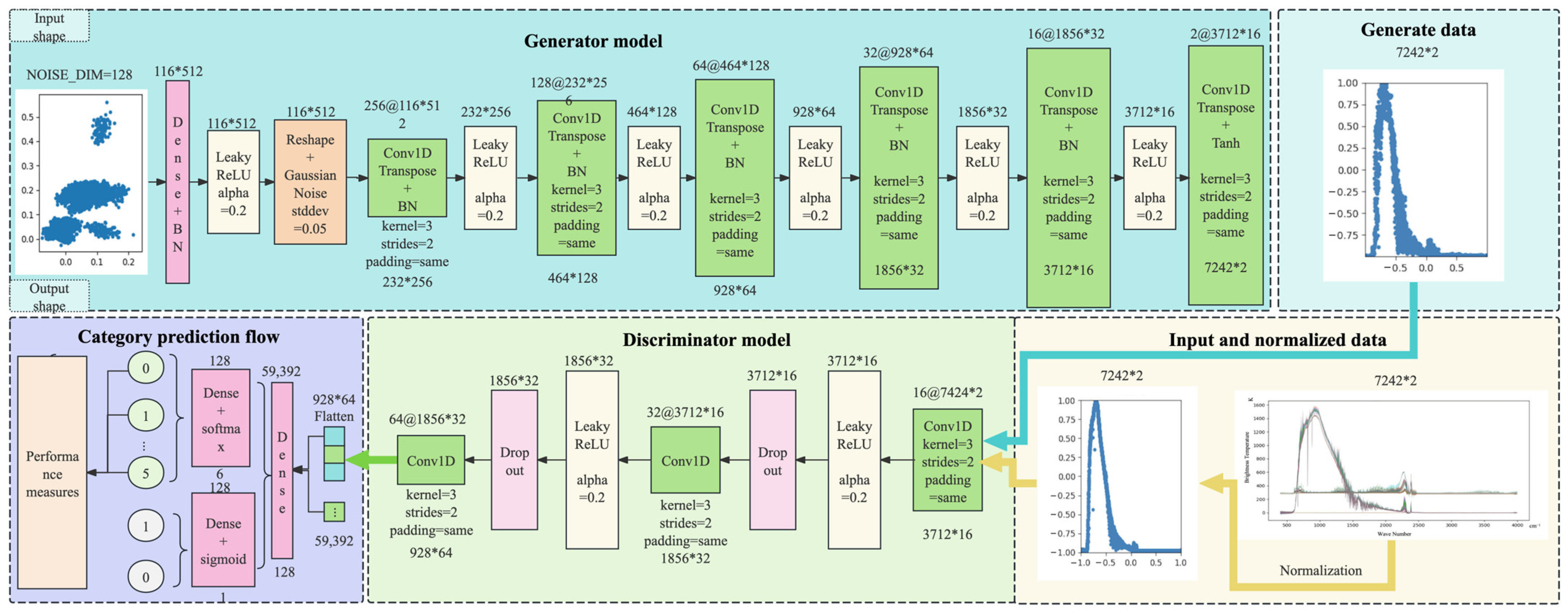
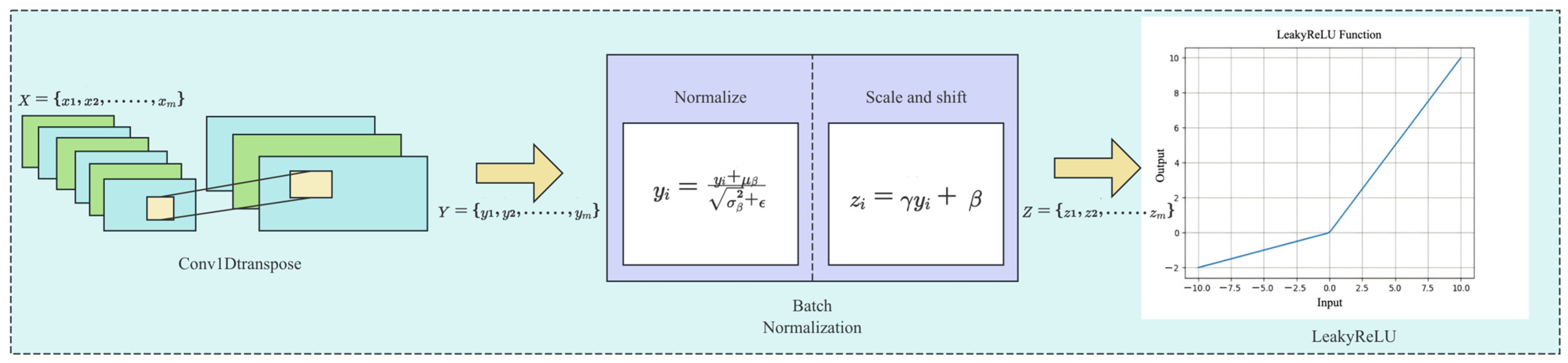
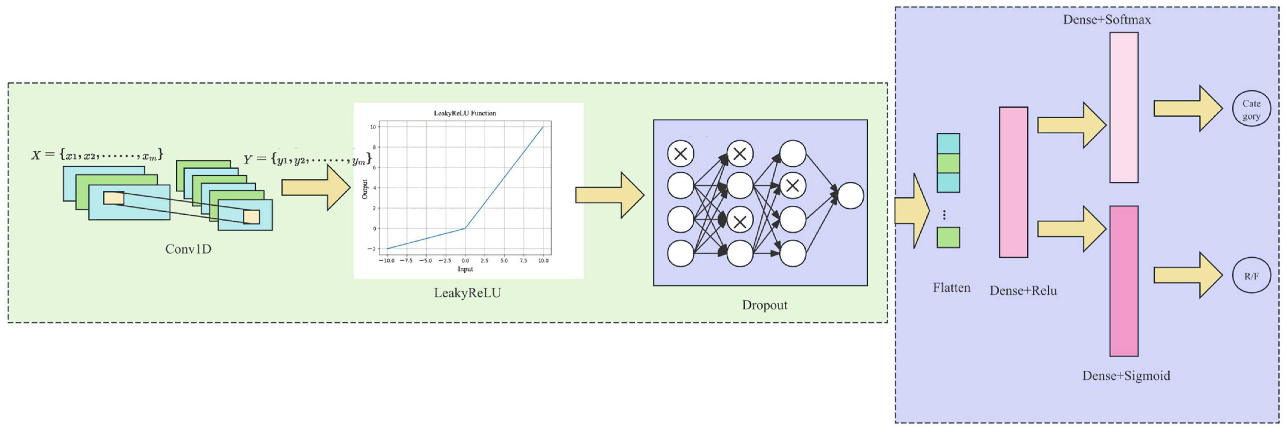
2.3.2. Network Composition Design
- 1.
- Generative Network
- 2.
- Discriminator Network
2.3.3. Network Training Methods
3. Experiment and Results
4. Discussion
4.1. Discussion on Comparative Experimental Results of Spectral Data Augmentation Methods
4.2. Discussion on the Ablation Experiment Results
5. Conclusions
Author Contributions
Funding
Data Availability Statement
Conflicts of Interest
References
- Li, S.; Song, W.; Fang, L.; Chen, Y.; Ghamisi, P.; Benediktsson, J.A. Deep Learning for Hyperspectral Image Classification: An Overview. IEEE Trans. Geosci. Remote Sens. 2019, 57, 6690–6709. [Google Scholar] [CrossRef]
- Shi, W.; Koo, D.E.S.; Kitano, M.; Chiang, H.J.; Trinh, L.A.; Turcatel, G.; Steventon, B.; Arnesano, C.; Warburton, D.; Fraser, S.E.; et al. Pre-processing visualization of hyperspectral fluorescent data with Spectrally Encoded Enhanced Representations. Nat. Commun. 2020, 11, 726. [Google Scholar] [CrossRef] [PubMed]
- Nalepa, J.; Myller, M.; Kawulok, M. Hyperspectral Data Augmentation. arXiv 2019, arXiv:1903.05580. [Google Scholar]
- Wang, K.; Gou, C.; Duan, Y.; Lin, Y.; Zheng, X.; Wang, F.-Y. Generative adversarial networks: Introduction and outlook. IEEE/CAA J. Autom. Sin. 2017, 4, 588–598. [Google Scholar] [CrossRef]
- Goodfellow, I.; Pouget-Abadie, J.; Mirza, M.; Xu, B.; Warde-Farley, D.; Ozair, S.; Courville, A.; Bengio, Y. GAN(Generative Adversarial Nets). J. Jpn. Soc. Fuzzy Theory Intell. Inform. 2017, 29, 177. [Google Scholar] [CrossRef]
- Mirza, M.; Osindero, S. Conditional Generative Adversarial Nets. arXiv 2014, arXiv:1411.1784. [Google Scholar]
- Radford, A.; Metz, L.; Chintala, S. Unsupervised Representation Learning with Deep Convolutional Generative Adversarial Networks. arXiv 2015, arXiv:1511.06434. [Google Scholar]
- Miyato, T.; Kataoka, T.; Koyama, M.; Yoshida, Y. Spectral Normalization for Generative Adversarial Networks. In Proceedings of the International Conference on Learning Representations, International Conference on Learning Representations, Vancouver, BC, Canada, 30 April–3 May 2018. [Google Scholar]
- Karras, T.; Laine, S.; Aila, T. A Style-Based Generator Architecture for Generative Adversarial Networks. In Proceedings of the 2019 IEEE/CVF Conference on Computer Vision and Pattern Recognition (CVPR), Long Beach, CA, USA, 15–20 June 2019. [Google Scholar] [CrossRef]
- He, Z.; Liu, H.; Wang, Y.; Hu, J. Generative Adversarial Networks-Based Semi-Supervised Learning for Hyperspectral Image Classification. Remote Sens. 2017, 9, 1042. [Google Scholar] [CrossRef]
- Zhan, Y.; Hu, D.; Wang, Y.; Yu, X. Semisupervised Hyperspectral Image Classification Based on Generative Adversarial Networks. IEEE Geosci. Remote Sens. Lett. 2018, 15, 212–216. [Google Scholar] [CrossRef]
- Zhu, L.; Chen, Y.; Ghamisi, P.; Benediktsson, J.A. Generative Adversarial Networks for Hyperspectral Image Classification. IEEE Trans. Geosci. Remote Sens. 2018, 56, 5046–5063. [Google Scholar] [CrossRef]
- Ding, F.; Guo, B.; Jia, X.; Chi, H.; Xu, W. Improving GAN-based feature extraction for hyperspectral images classification. J. Electron. Imaging 2021, 30, 063011. [Google Scholar] [CrossRef]
- Ranjan, P.; Girdhar, A.; Ankur, R.; Kumar, R. A novel spectral-spatial 3D auxiliary conditional GAN integrated convolutional LSTM for hyperspectral image classification. Earth Sci. Inform. 2024, 17, 5251–5271. [Google Scholar] [CrossRef]
- Wang, J.; Gao, F.; Dong, J.; Du, Q. Adaptive DropBlock-Enhanced Generative Adversarial Networks for Hyperspectral Image Classification. IEEE Trans. Geosci. Remote Sens. 2021, 59, 5040–5053. [Google Scholar] [CrossRef]
- Li, W.; Chen, C.; Zhang, M.; Li, H.; Du, Q. Data Augmentation for Hyperspectral Image Classification With Deep CNN. IEEE Geosci. Remote Sens. Lett. 2019, 16, 593–597. [Google Scholar] [CrossRef]
- Haut, J.M.; Paoletti, M.E.; Plaza, J.; Plaza, A.; Li, J. Hyperspectral Image Classification Using Random Occlusion Data Augmentation. IEEE Geosci. Remote Sens. Lett. 2019, 16, 1751–1755. [Google Scholar] [CrossRef]
- Wang, W.; Liu, X.; Mou, X. Data Augmentation and Spectral Structure Features for Limited Samples Hyperspectral Classification. Remote Sens. 2021, 13, 547. [Google Scholar] [CrossRef]
- Gao, H.; Zhang, J.; Cao, X.; Chen, Z.; Zhang, Y.; Li, C. Dynamic Data Augmentation Method for Hyperspectral Image Classification Based on Siamese Structure. IEEE J. Sel. Top. Appl. Earth Obs. Remote Sens. 2021, 14, 8063–8076. [Google Scholar] [CrossRef]
- Du, S.; Han, W.; Kang, Z.; Lu, X.; Liao, Y.; Li, Z. Continuous Wavelet Transform Peak-Seeking Attention Mechanism Conventional Neural Network: A Lightweight Feature Extraction Network with Attention Mechanism Based on the Continuous Wave Transform Peak-Seeking Method for Aero-Engine Hot Jet Fourier Transform Infrared Classification. Remote Sens. 2024, 16, 3097. [Google Scholar] [CrossRef]
- Elaraby, S.; Sabry, Y.M.; Abuelenin, S.M. Super-resolution infrared spectroscopy for gas analysis using convolutional neural networks. In Applications of Machine Learning 2020; SPIE: Bellingham, WA, USA, 2020. [Google Scholar] [CrossRef]
- Mao, M.; Cao, Y.; Ni, P.; Li, Z.; Zhang, X. Quantitative Analysis of Infrared Spectroscopy of Alkane Gas Based on Random Forest Algorithm. In Proceedings of the 2023 5th International Conference on Intelligent Control, Measurement and Signal Processing (ICMSP), Chengdu, China, 19–21 May 2023; pp. 1166–1170. [Google Scholar] [CrossRef]
- Wang, Y.-H.; Liu, J.-G.; Xu, L.; Cheng, X.-X.; Deng, Y.-S.; Shen, X.-C.; Sun, Y.-F.; Xu, H.-Y. Qualitative Analysis of the Gas Detection Limit of Fourier Infrared Spectroscopy. Acta Phys. Sin. 2022, 71, 093201. [Google Scholar] [CrossRef]
- Doubenskaia, M.; Pavlov, M.; Grigoriev, S.; Smurov, I. Definition of brightness temperature and restoration of true temperature in laser cladding using infrared camera. Surf. Coat. Technol. 2013, 220, 244–247. [Google Scholar] [CrossRef]
- Homan, D.C.; Cohen, M.H.; Hovatta, T.; Kellermann, K.I.; Kovalev, Y.Y.; Lister, M.L.; Popkov, A.V.; Pushkarev, A.B.; Ros, E.; Savolainen, T. MOJAVE. XIX. Brightness Temperatures and Intrinsic Properties of Blazar Jets. Astrophys. J. 2021, 923, 67. [Google Scholar] [CrossRef]
- Chu, P.M.; Guenther, F.R.; Rhoderick, G.C.; Lafferty, W.J. The NIST Quantitative Infrared Database. J. Res. Natl. Inst. Stand. Technol. 1999, 104, 59. [Google Scholar] [CrossRef]
- Dumoulin, V.; Visin, F. A guide to convolution arithmetic for deep learning. arXiv 2016, arXiv:1603.07285. [Google Scholar]
- Ioffe, S.; Szegedy, C. Batch Normalization: Accelerating Deep Network Training by Reducing Internal Covariate Shift. arXiv 2015, arXiv:1502.03167. [Google Scholar]
- Xu, J.; Li, Z.; Du, B.; Zhang, M.; Liu, J. Reluplex made more practical: Leaky ReLU. In Proceedings of the 2020 IEEE Symposium on Computers and Communications (ISCC), Rennes, France, 8–10 July 2020. [Google Scholar] [CrossRef]
- Srivastava, N.; Hinton, G.; Krizhevsky, A.; Sutskever, I.; Salakhutdinov, R. Dropout: A simple way to prevent neural networks from overfitting. J. Mach. Learn. Res. 2014, 15, 1929–1958. [Google Scholar]
- Glorot, X.; Bordes, A.; Bengio, Y. Deep Sparse Rectifier Neural Networks. J. Mach. Learn. Res. 2011, 15, 275. [Google Scholar]
- Qin, Y.; Mitra, N.; Wonka, P. How does Lipschitz Regularization Influence GAN Training? In Proceedings of the Computer Vision—ECCV 2020, Glasgow, UK, 23–28 August 2020; Lecture Notes in Computer Science. Springer: Berlin/Heidelberg, Germany, 2020; pp. 310–326. [Google Scholar] [CrossRef]
- Salimans, T.; Goodfellow, I.; Zaremba, W.; Cheung, V.; Radford, A.; Chen, X. Improved Techniques for Training GANs. arXiv 2016, arXiv:1606.03498. [Google Scholar]
- Brock, A.; Donahue, J.; Simonyan, K. Large Scale GAN Training for High Fidelity Natural Image Synthesis. In Proceedings of the International Conference on Learning Representations, International Conference on Learning Representations, Vancouver, BC, Canada, 30 April–3 May 2018. [Google Scholar]
- Kingma, D.P.; Ba, J. Adam: A Method for Stochastic Optimization. arXiv 2014, arXiv:1412.6980. [Google Scholar]
- Shorten, C.; Khoshgoftaar, T.M. A survey on Image Data Augmentation for Deep Learning. J. Big Data 2019, 6, 1–48. [Google Scholar] [CrossRef]
- Chen, X.; Sun, Y.; Zhang, M.; Peng, D. Evolving Deep Convolutional Variational Autoencoders for Image Classification. IEEE Trans. Evol. Comput. 2021, 25, 815–829. [Google Scholar] [CrossRef]

| Name | Measurement Pattern | Spectral Resolution (cm−1) | Spectral Measurement Range (µm) | Full Field of View Angle |
|---|---|---|---|---|
| EM27 | Active/Passive | Active: 0.5/1; Passive: 0.5/1/4 | 2.5~12 | 30 mrad (no telescope) (1.7°) |
| Telemetry Fourier Transform Infrared Spectrometer | Passive | 1 | 2.5~12 | 1.5° |
| Serial Number | Class | Type | Number of Data Pieces | Full Band Data Volume |
|---|---|---|---|---|
| 1 | C 0 | Aero-Engine 1 (Turbofan) | 256 | 16384 |
| 2 | C 1 | Aero-Engine 2 (Turbojet) | 48 | 16384 |
| 3 | C 2 | Aero-Engine 3 (Turbofan) | 712 | 16384 |
| 4 | C 3 | Aero-Engine 4 (Turbojet) | 199 | 16384 |
| 5 | C 4 | Aero-Engine 5 (Turbojet) | 380 | 16384 |
| 6 | C 5 | Aero-Engine 6 (Turbojet) | 193 | 16384 |
| Serial Number | Class | Environmental Temperature | Environmental Humidity | Detection Distance |
|---|---|---|---|---|
| 1 | C 0 | 19 °C | 58.5% Rh | 5 m |
| 2 | C 1 | 16 °C | 67% Rh | 5 m |
| 3 | C 2 | 14 °C | 40% Rh | 5 m |
| 4 | C 3 | 30 °C | 43.5% Rh | 11.8 m |
| 5 | C 4 | 20 °C | 71.5% Rh | 5 m |
| 6 | C 5 | 19 °C | 73.5% Rh | 10 m |
| DATA SET | Data Volume | Category Proportion % | Select Range Data Volume | |||||
|---|---|---|---|---|---|---|---|---|
| C 0 | C 1 | C 2 | C 3 | C 4 | C 5 | |||
| Training set | 1432 (80%) | 14.66 | 2.93 | 39.59 | 11.31 | 20.67 | 10.82 | 7424 |
| Validation set | 178 (10%) | 10.67 | 1.69 | 43.26 | 10.11 | 26.97 | 7.30 | 7424 |
| Prediction set | 178 (10%) | 15.17 | 1.69 | 38.2 | 10.67 | 20.22 | 14.04 | 7424 |
| Layers | Parameter Settings |
|---|---|
| Input | input_shape = (7424, 2),num_classes = 6 |
| Network parameter settings | EPOCHS = 500, BATCH_SIZE = 128, NOISE_DIM = 128, LEARNING_RATE_G = 0.0001, LEARNING_RATE_D = 0.0005, CHANNEL_1 = 16, CHANNEL_2 = 32, CHANNEL_3 = 64, CHANNEL_4 = 128, CHANNEL_5 = 256, CHANNEL_6 = 512 |
| Generator | Dense((data_shape_x // 64) * CHANNEL_6), BatchNormalization(), LeakyReLU(), Reshape((data_shape_x // 64, CHANNEL_6)) CHANNEL_5 to CHANNEL_1: Conv1DTranspose(CHANNEL, kernel_size = 3, strides = 2, padding = ‘same’),BatchNormalization(), LeakyReLU() Conv1DTranspose(2, kernel_size = 3, strides = 2, padding = ‘same’, activation = ‘tanh’) |
| Discriminator | CHANNEL_1 to CHANNEL_3: Conv1D(CHANNEL, kernel_size = 3, strides = 2, padding = ‘same’) LeakyReLU(), Dropout(0.3), Flatten()(x) Dense(128, activation = ‘relu’) Dense(num_classes, activation = ‘softmax’, name = ‘class_output’) Dense(1, activation = ‘sigmoid’, name = ‘validity_output’) |
| Evaluation Criterion | Accuracy | Precision | Recall | F1-Score | |
|---|---|---|---|---|---|
| Methods | |||||
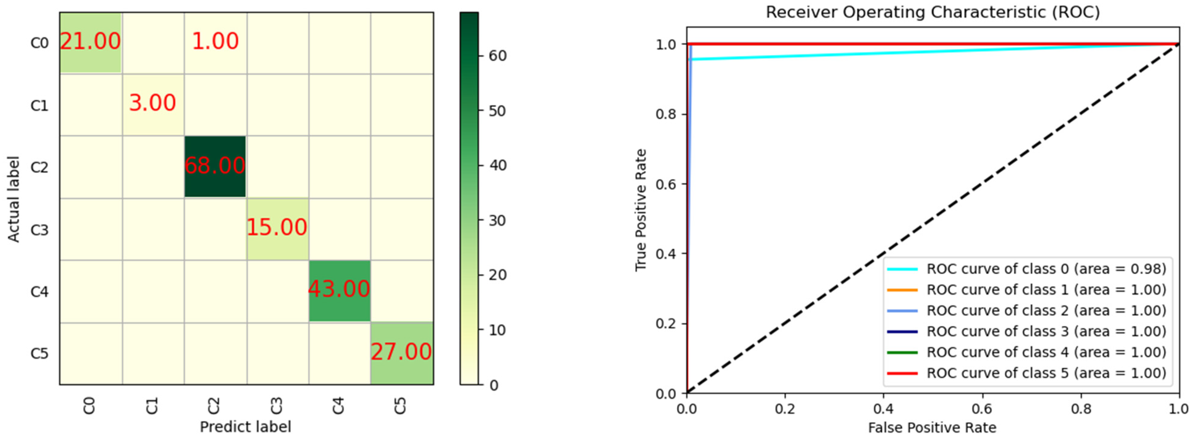
| FTIR-SpectralGAN | 99.44% | 99.76% | 99.24% | 99.49% | |
| Methods | Parameter Settings | Data Augmentation Methods | ||
|---|---|---|---|---|
| Data Augmentation | CNN | CHANNEL_1 to CHANNEL_3: Conv1D(CHANNEL, kernel_size = 3, strides = 2, padding = ‘same’) LeakyReLU(), Dropout(0.3) Flatten()(x) Dense(128, activation = ‘relu’) Dense(num_classes, activation = ‘softmax’) Dense(1, activation = ‘sigmoid’) | Methods | Parameter Settings |
| Rotation | Random rotation (0, 2 π) | |||
| Scaling | Random scale (0.8, 1.2) | |||
| Translation | Max translation = 0.1 | |||
| Resampling | Samples = 50 | |||
| Reflection | Random reflection | |||
| Jitter | Noise level = 0.05 Decimal places = 2 | |||
| Dropout | Dropout rate =0.1 | |||
| Data Synthetic | CVAE | CHANNEL_1 = 32, CHANNEL_2 = 16, CHANNEL_3 = 8, CHANNEL_OUTPUT = 1 Encoded: (CHANNEL_1 to CHANNEL_3) Conv1D (kernel_size = 3, activation = ‘Tanh’, padding = ‘same’, kernel_regularizer = l2(0.01)), MaxPooling1D (2, padding = ‘same’) Latent space:Dense (z_mean),Dense (z_log_var), Lambda (z = z_mean + tf.exp (0.5 × z_log_var) × epsilon) Decoded: (CHANNEL_3 to CHANNEL_1) Conv1DTranspose (kernel_size = 3, strides = 1, activation = ‘Tanh’, padding = ‘same’), UpSampling1D(2) Flatten = Flatten(),Dense (num_classes, activation = ‘softmax’) optimizer = tf.keras.optimizers.Adam (lr = 0.0001) loss = [‘mse’, ‘sparse_categorical_crossentropy’], loss_weights = [0.5, 0.5] epochs = 500, batch size = 64 | ||
| Spectral Feature | PCA +SVM | PCA(n_components = 0.95), Svm = SVC(kernel = ‘rbf’, C = 10, gamma = 0.01) | ||
| CO2 +XGBoost | objective = ‘multi:softmax’ estimators = 500 estimators = 500 | |||
| CO2+ Random Forest | estimators = 500 | |||
| Evaluation Criterion | Accuracy | Precision | Recall | F1-Score | |
|---|---|---|---|---|---|
| Method | |||||
| Data Augmentation | CNN | 96.09% | 98.72% | 94.70% | 96.18% |
| Rotation + CNN | 96.65% | 98.89% | 95.45% | 96.79% | |
| Scaling + CNN | 99.44% | 99.80% | 99.24% | 99.51% | |
| Translation + CNN | 96.09% | 98.72% | 94.70% | 96.18% | |
| Resampling + CNN | 96.09% | 98.72% | 94.70% | 96.18% | |
| Reflection + CNN | 96.09% | 98.72% | 94.70% | 96.18% | |
| Jitter + CNN | 96.65% | 98.89% | 95.45% | 96.79% | |
| Dropout + CNN | 96.09% | 98.72% | 94.70% | 96.18% | |
| Data Synthetic | FTIR-SpectralGAN | 99.44% | 99.76% | 99.24% | 99.49% |
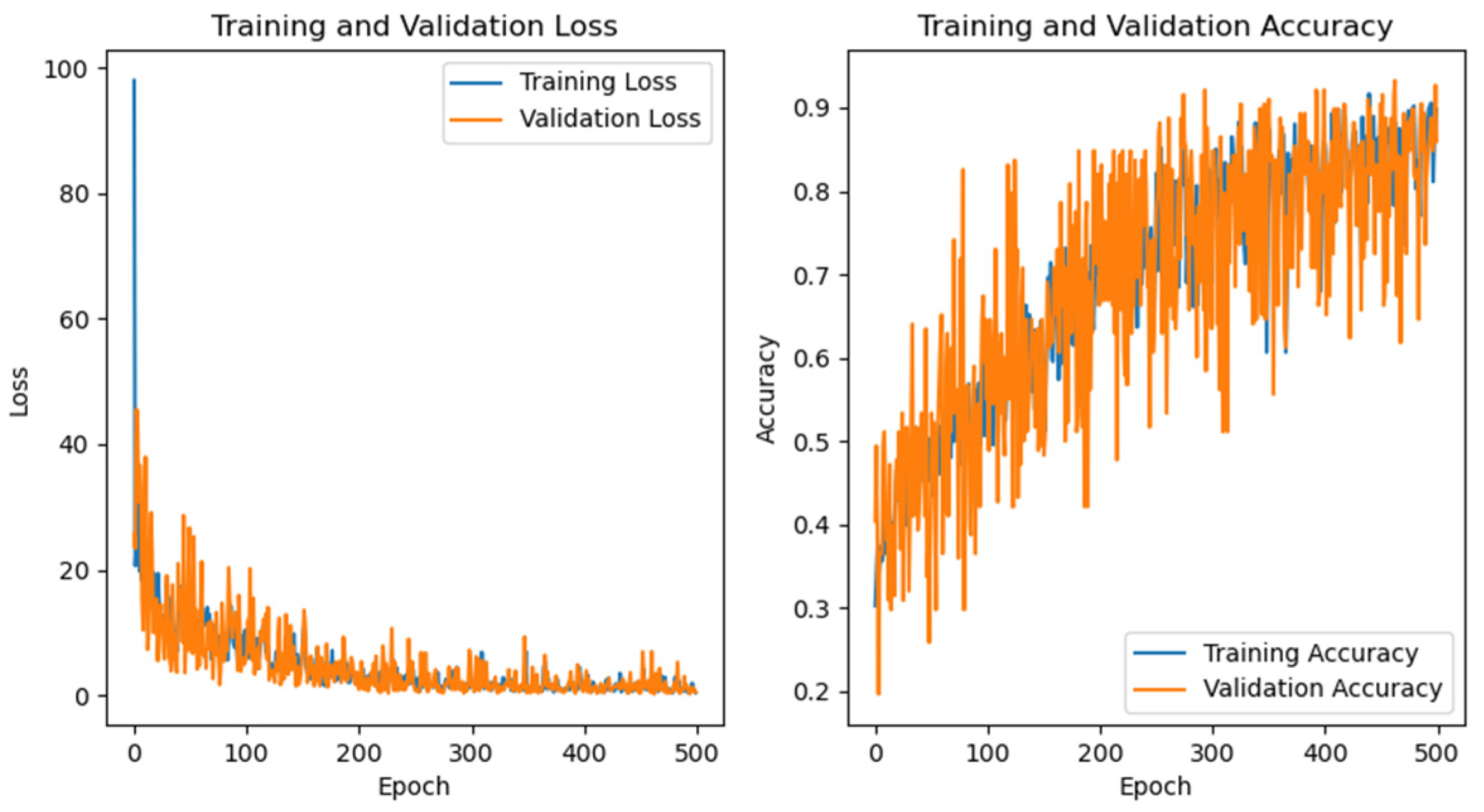
| CVAE | 84.35% | 84.85% | 84.27% | 83.85% | |
| Spectral Feature | PCA + SVM | 93.82% | 90.51% | 88.71% | 89.34% |
| CO2 + XGBoost | 94.41% | 91.75% | 93.33% | 92.43% | |
| CO2+ Random Forest | 94.97% | 92.38% | 94.49% | 93.2% |
| Methods | Train Time/s | Prediction Time/s |
|---|---|---|
| CNN | 959.04 | 0.23 |
| Rotation + CNN | 2197.84 | 0.20 |
| Scaling + CNN | 2151.22 | 0.19 |
| Translation + CNN | 2181.78 | 0.18 |
| Resampling + CNN | 2089.91 | 0.19 |
| Reflection + CNN | 2111.77 | 0.20 |
| Jitter + CNN | 2159.05 | 0.19 |
| Dropout + CNN | 2123.13 | 0.19 |
| FTIR-SpectralGAN | 4661.46 | 0.35 |
| CVAE | 1790.76 | 2.25 |
| PCA + SVM | 1.1060 | 0.0588 |
| CO2 + XGBoost | 1.3269 | 0.5523 |
| CO2+ Random Forest | 0.8447 | 0.4293 |
| Evaluation Criterion | Accuracy | Precision Score | Recall | F1-Score | |
|---|---|---|---|---|---|
| Method | |||||
| CNN | 89.94% | 97.06% | 86.36% | 86.85% | |
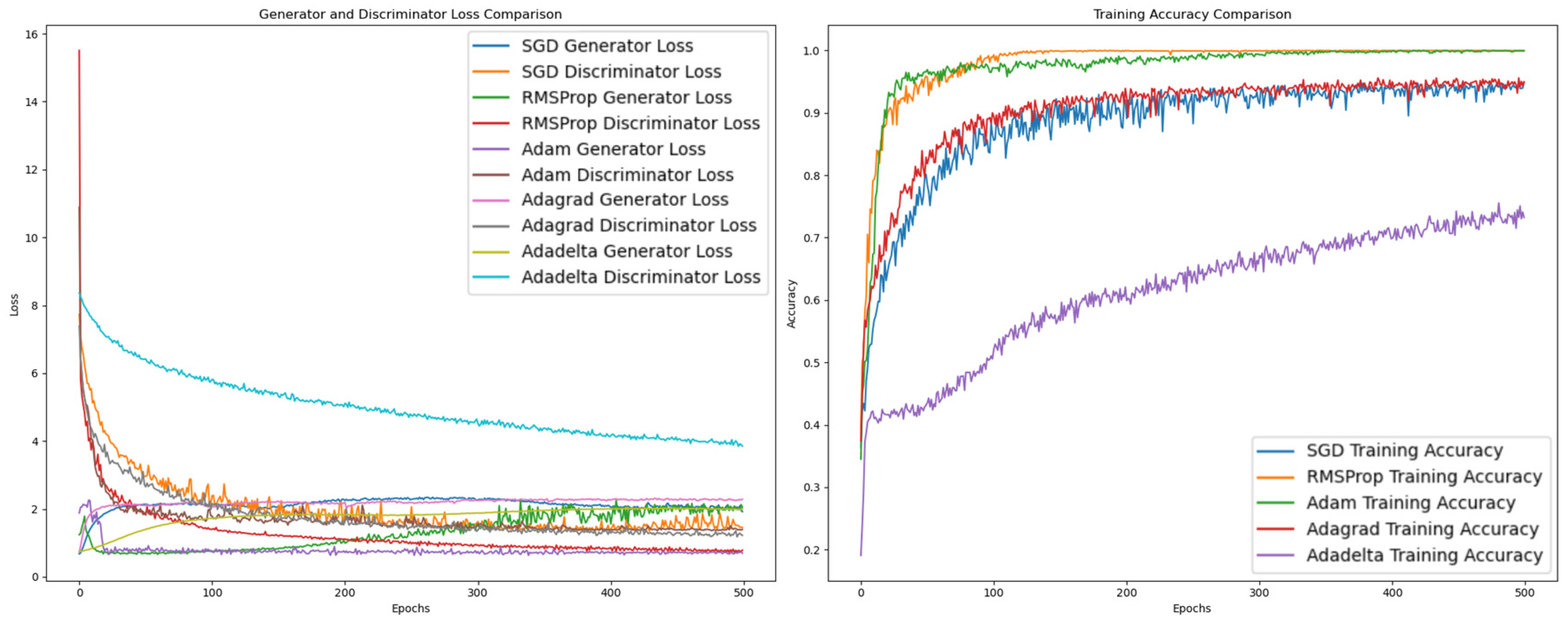
| Optimizers | Accuracy | Training Time/s | Prediction Time/s | Confusion Matrix | ROC |
|---|---|---|---|---|---|
| SGD | 94% | 4434.86 | 0.74 | 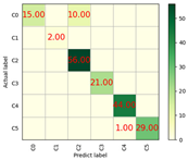 | 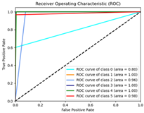 |
| RMSProp | 98% | 4774.95 | 1.59 | 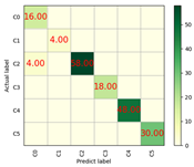 | 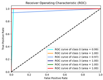 |
| Adam | 100% | 4515.55 | 0.70 | 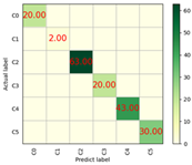 | 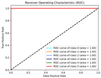 |
| Adagrad | 97% | 4565.57 | 0.73 | 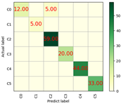 | 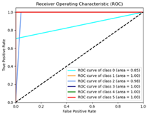 |
| Adadelta | 71% | 4599.13 | 0.64 | 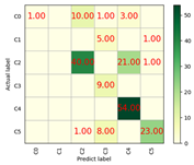 | 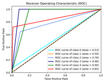 |
Disclaimer/Publisher’s Note: The statements, opinions and data contained in all publications are solely those of the individual author(s) and contributor(s) and not of MDPI and/or the editor(s). MDPI and/or the editor(s) disclaim responsibility for any injury to people or property resulting from any ideas, methods, instructions or products referred to in the content. |
© 2025 by the authors. Licensee MDPI, Basel, Switzerland. This article is an open access article distributed under the terms and conditions of the Creative Commons Attribution (CC BY) license (https://creativecommons.org/licenses/by/4.0/).
Share and Cite
Du, S.; Liao, Y.; Feng, R.; Luo, F.; Li, Z. FTIR-SpectralGAN: A Spectral Data Augmentation Generative Adversarial Network for Aero-Engine Hot Jet FTIR Spectral Classification. Remote Sens. 2025, 17, 1042. https://doi.org/10.3390/rs17061042
Du S, Liao Y, Feng R, Luo F, Li Z. FTIR-SpectralGAN: A Spectral Data Augmentation Generative Adversarial Network for Aero-Engine Hot Jet FTIR Spectral Classification. Remote Sensing. 2025; 17(6):1042. https://doi.org/10.3390/rs17061042
Chicago/Turabian StyleDu, Shuhan, Yurong Liao, Rui Feng, Fengkun Luo, and Zhaoming Li. 2025. "FTIR-SpectralGAN: A Spectral Data Augmentation Generative Adversarial Network for Aero-Engine Hot Jet FTIR Spectral Classification" Remote Sensing 17, no. 6: 1042. https://doi.org/10.3390/rs17061042
APA StyleDu, S., Liao, Y., Feng, R., Luo, F., & Li, Z. (2025). FTIR-SpectralGAN: A Spectral Data Augmentation Generative Adversarial Network for Aero-Engine Hot Jet FTIR Spectral Classification. Remote Sensing, 17(6), 1042. https://doi.org/10.3390/rs17061042