Abstract
The high-precision motion state analysis of space targets has important scientific value and application potential in the fields of geodynamics, geodesy, space collision warning and avoidance, and the capture, recovery, and removal of space debris. With the increasing repetition rate of satellite laser ranging systems, the inversion and analysis of space target motion state based on high-precision and high-repetition-rate satellite laser ranging data has become a hot spot in current research. How to filter out noise and retain valid information from the high-repetition-rate, high-precision laser ranging data has become a challenge. The traditional polynomial fitting method has problems with low data accuracy and erroneous deletion of valid data when processing laser ranging data with complex patterns. To address this problem, this paper innovatively designs a new type of spline function and accordingly proposes a laser ranging data preprocessing method that can automatically adapt to the trend of data variation. The method is validated using various characteristic observation data provided by Changchun station (7237), and the results show that the novel spline method is superior to the traditional method in maintaining the integrity of data patterns and significantly improves the data accuracy. After two iterations of denoising, the RMS of the novel spline method is reduced to one-fourth of that before denoising and as low as one-eighteenth of that of the traditional method, and the accuracy is further improved with the increase of the number of iterations. This study provides a practical and reliable novel solution for the preprocessing of laser ranging data with complex patterns.
1. Introduction
Satellite laser ranging (SLR) is the most precise space geodetic technique for single-point measurement, and dozens of stations around the world of the International Laser Ranging Service (ILRS) work together to conduct joint observation of space targets. And utilizing SLR data, we can obtain many scientific products [1,2,3,4], such as precise geocentric positions and motions of ground stations, components of the Earth’s gravity field and their temporal variations, Earth orientation parameters (EOPs), precision orbit of satellites, etc. With the advancement of laser ranging technology, especially the increasing frequency of laser ranging systems [5,6,7,8], and the research and experimentation of laser ranging systems with frequencies up to 100 kHz and above in recent years [9,10,11,12], SLR is not only able to provide accurate distance information but also has the data conditions necessary for high-precision inversion of the motion state of space targets [13]. Scholars, such as Tang Rufeng [14], Liu Tong [15], and Kucharski [16], have already conducted research on the motion state of the Ajisai satellite based on the high repetition rate satellite laser ranging data. In addition, space debris poses a serious threat to the safety of spacecraft in orbit, and frequent collision events necessitate the use of high-precision observational data for orbit determination and attitude analysis of space debris [17,18,19]. In recent years, SLR technology has been successfully applied to the high-precision detection of non-cooperative targets [20,21,22,23], and the motion state of non-cooperative targets has been analyzed and studied. For example, Kucharski et al. investigated the spin rate and spin axis orientation of non-cooperative targets such as Topex and Envisat using laser ranging data [24,25,26], while Liu Tong et al. estimated the rocket debris tumbling attitude based on laser ranging data [27]. These high-precision motion state analyses of cooperative and non-cooperative targets are not only of significant scientific value to the fields of geodynamics and geodesy [28,29], such as the estimation of SLR station coordinates and Earth’s elastic parameters, but also provide critical support for the improvement of orbital perturbation modeling of space targets and for the applications of tracking and monitoring, collision warning and avoidance, capture recovery, and removal of space debris [30,31,32,33,34,35].
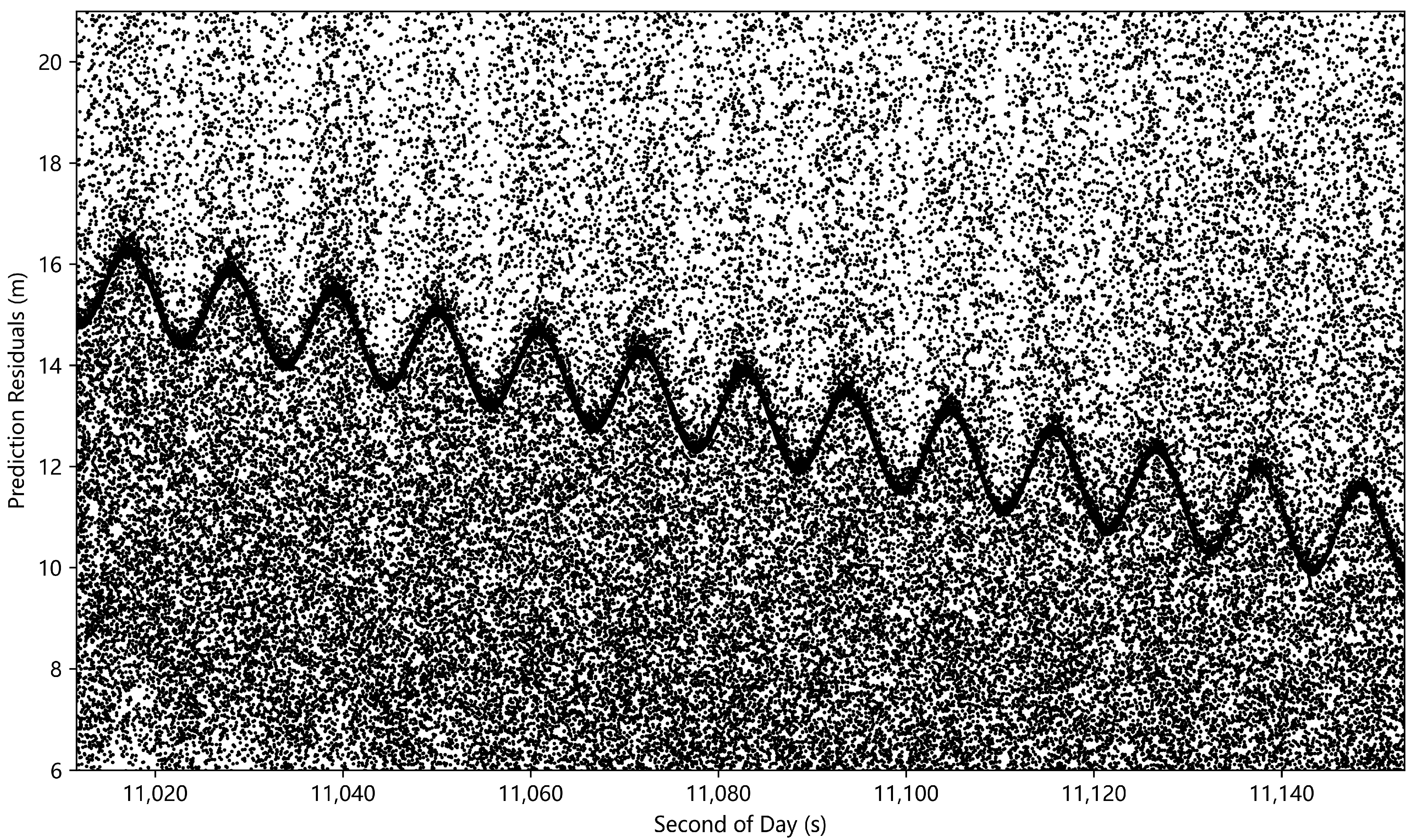
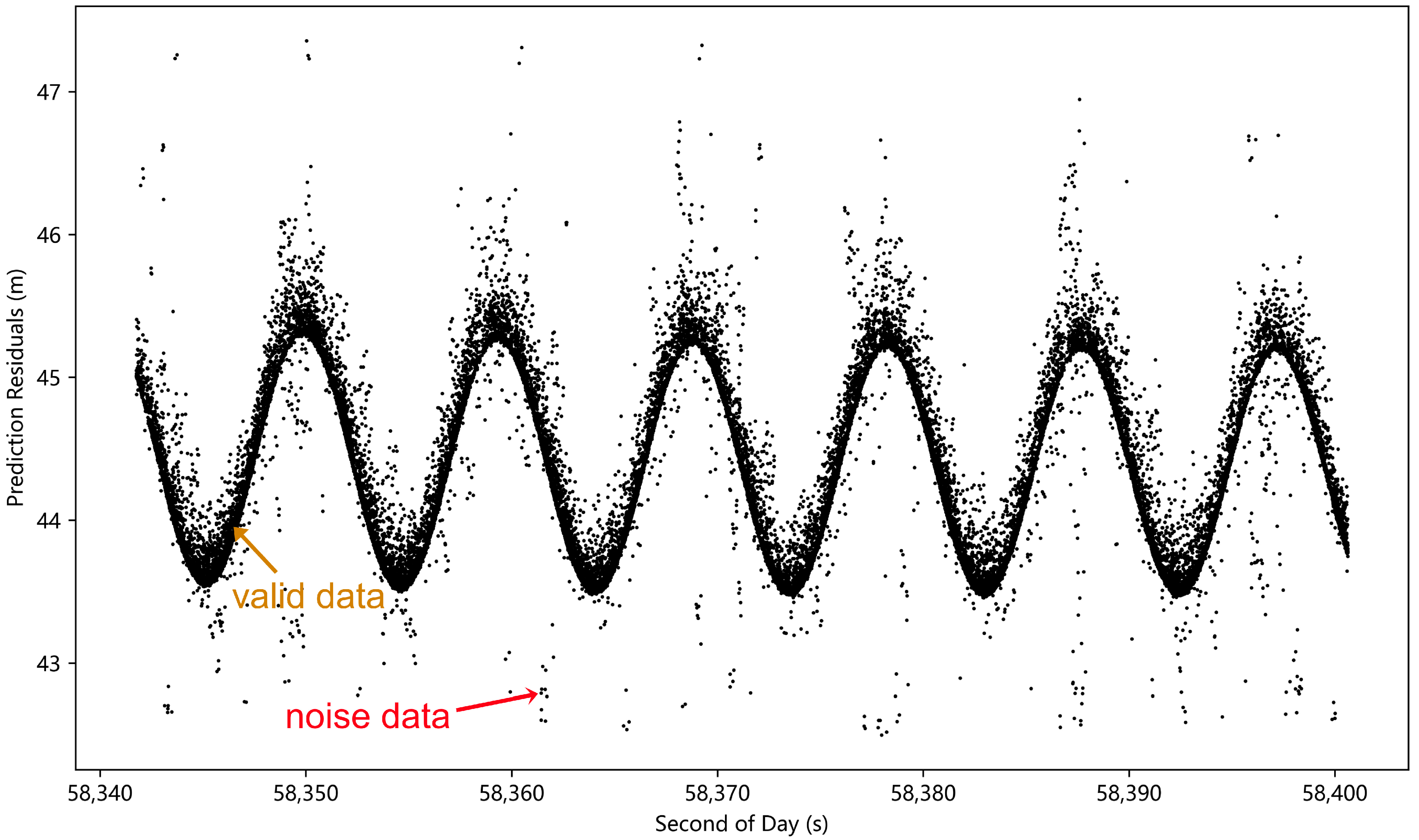
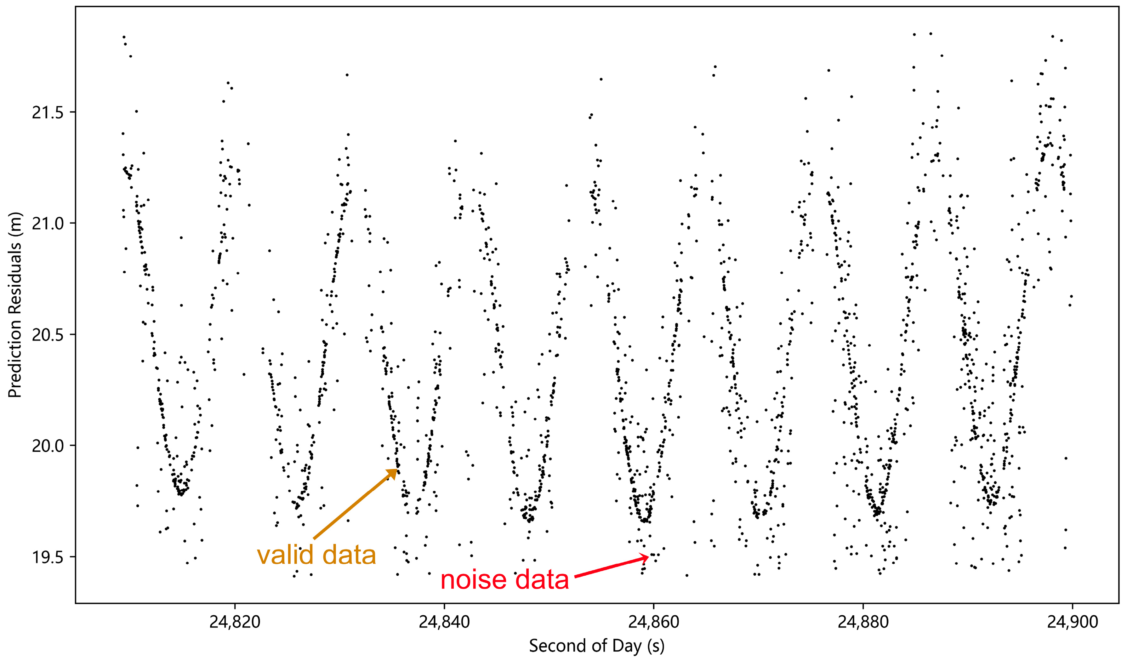
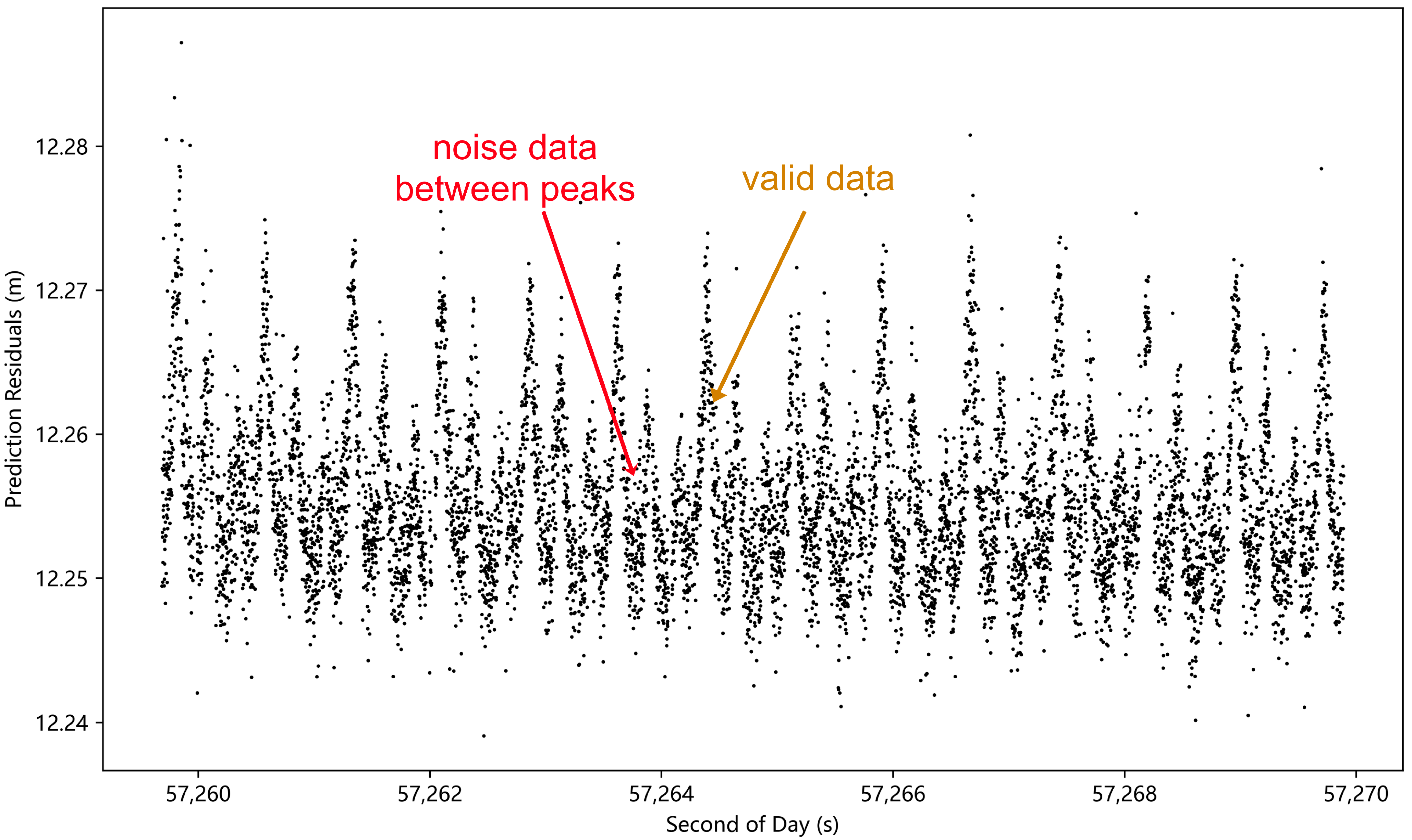
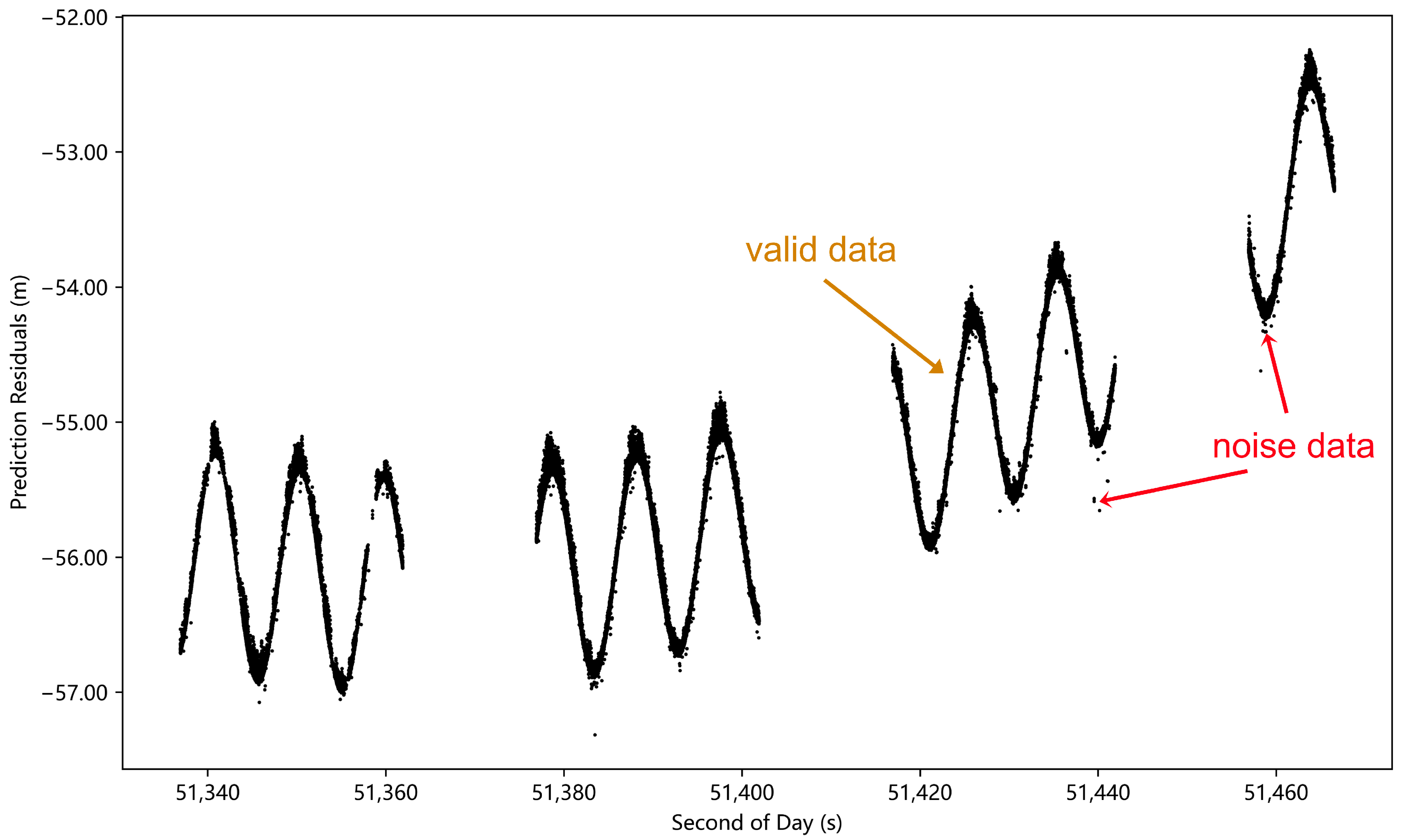
In terms of data processing, the raw SLR observation data represent the distance between the station and the target. Due to the large variation range of this distance value during the observation process, it is inconvenient to analyze this data directly. Therefore, before data preprocessing, the observed data (Observed) are usually subtracted from the theoretical prediction data (Computed) to obtain the prediction residual data (denoted by PR), i.e., O-C data, which are then preprocessed [36]. Under the dual influence of the complex space environment and the target’s own structural characteristics, some of the measured space targets show complex motion patterns, and their prediction residual data are characterized by intricate and variable oscillation patterns. In addition, due to the interference of factors such as the sky background and the detector’s own performance, the observation data contain a large amount of noise, as shown in Figure 1, especially in the case of low signal-to-noise ratios, and these noisy data can significantly affect the calculation accuracy of the target’s spin phase, spin rate, and other key motion parameters [37]. In view of this, it is necessary to conduct meticulous data preprocessing before in-depth analysis and application of laser ranging data to effectively remove noise and improve the accuracy of the data. In this process, it is also essential to ensure that the original patterns of the data are maintained and not distorted by the preprocessing. Therefore, the selection of appropriate data preprocessing methods is crucial.
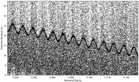
Figure 1.
High-repetition-rate laser ranging data prediction residuals.
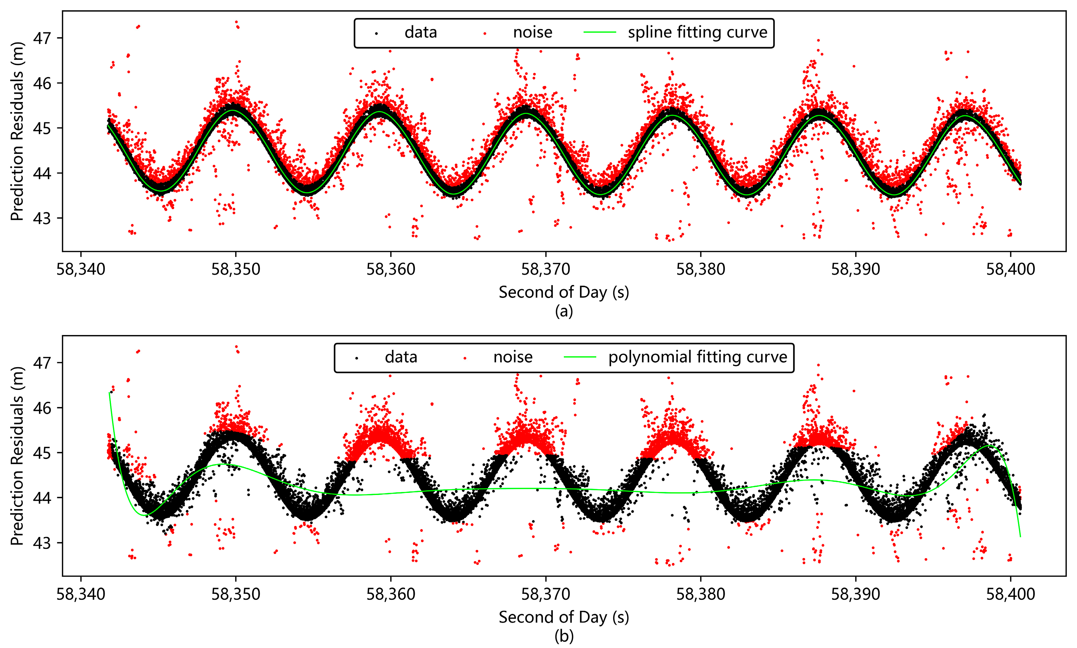
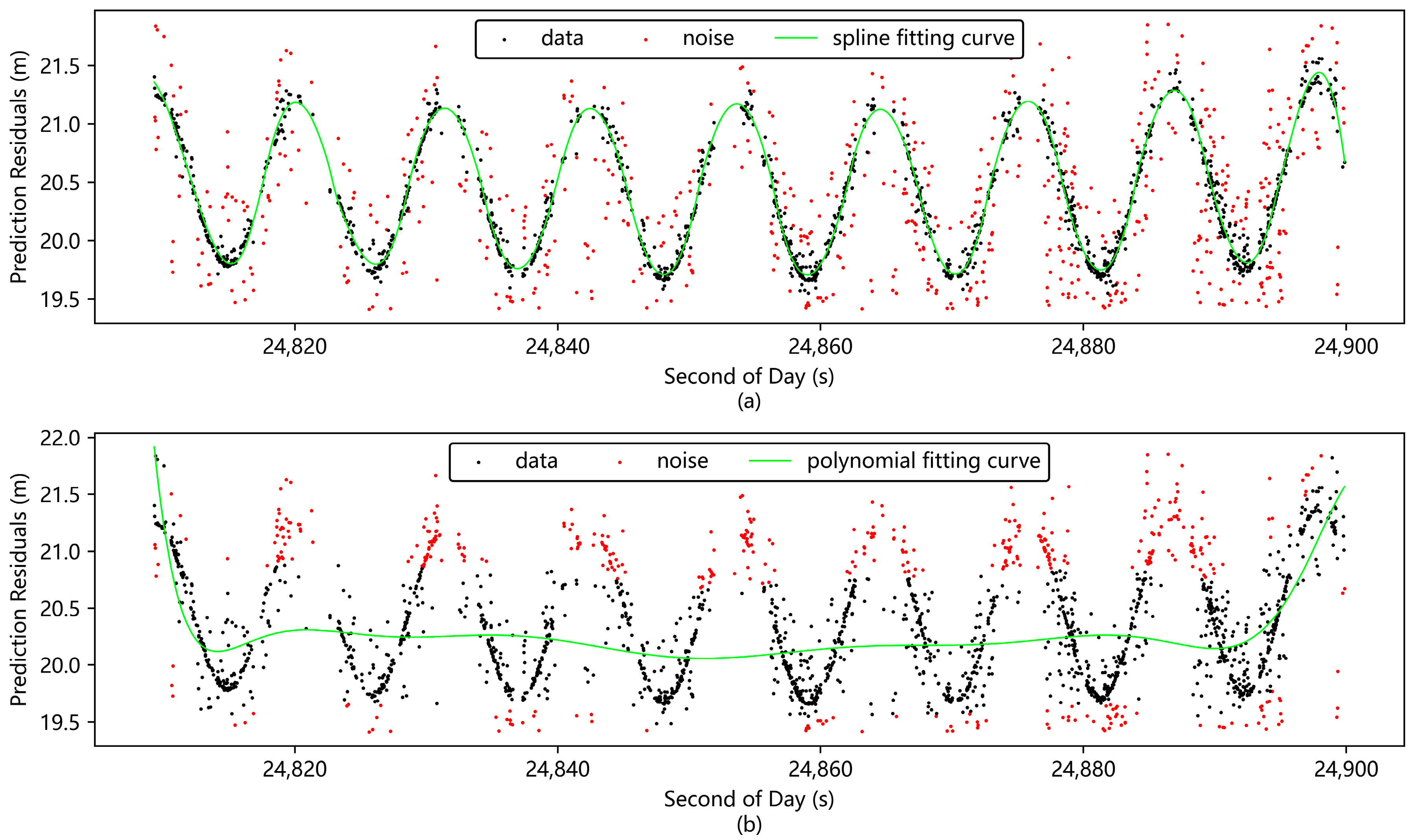
For the data preprocessing of conventional space targets, it is common to use manual noise rejection or automatic data identification techniques (e.g., Graz station’s fast identification algorithm, Poisson filtering, etc.) to realize the initial coarse filtering of data [38,39,40,41], and this coarse filtering means can effectively remove the noise away from the effective data band, but as shown in Figure 2, there still exists the residual noise near the effective data band. In this case, the traditional practice is to use polynomial fitting filtering for the fine rejection of noise [41,42,43]; this method is effective in dealing with laser ranging data for space targets with simpler motion states, less data volume, or less stringent requirements on data details. However, with the increase of the repetition rate of the laser ranging system and the increase of the information carried in the observation data, the researchers pay more attention to the subtle change patterns of the data in order to excavate the latent information in the data and use this information to carry out more in-depth scientific research. The ability of the polynomial fitting method to extract the patterns of data variation depends on its number; theoretically, the higher the number, the stronger the ability, but too high of a number will lead to data overfitting, so the number of polynomials will not be too high. In this case, when confronted with complex oscillatory patterns in prediction residuals, its limitations become evident as it cannot fully express the data’s variation patterns and is prone to mistakenly removing valid data during the noise reduction process, thus damaging the original data patterns. For such data, more targeted processing methods are needed.
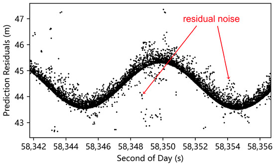
Figure 2.
Data after coarse filtering and residual noise.
A spline curve, due to its characteristics of no specific mathematical model, can flexibly adapt to data variations, approximate complex functional relationships, and eliminate the dependence of the data on the choice of model [44]. This ensures consistency between the curve and the data, meeting the demand for accurately describing the complex variation patterns of prediction residuals in space target observation data. However, the traditional spline function applies to a set of data with a specific pattern and constructs the spline curve by taking all the given data as spline nodes [45]. The prediction residual of laser ranging data is a banded dataset with a certain width and containing a large amount of noise [46], and although the data as a whole show a certain regular trend, any two adjacent data points in the dataset are independent of each other and do not have a specific mathematical relationship. The traditional spline curve construction method takes all prediction residual data, including noise, as nodes, resulting in the curve that do not fit as expected. Furthermore, the solution process for traditional spline functions requires preset boundary conditions, which are unknown for prediction residual data. To address the limitations of traditional spline functions, this paper designs a novel spline function without spline nodes and boundary conditions and develops a laser ranging data preprocessing method based on this function that adapts to the trend of data variation. This method can automatically identify the peaks, troughs, and discontinuity points in the prediction residual data and segment the global data according to these key feature points, with simple data patterns in each sub-segment, which realizes the simplicity of complex patterns and overcomes the limitations of the traditional polynomial fitting method. Then, the segmented data with simple patterns are processed by best fitting to obtain segmented fitting functions, and a bridging function is used to smoothly connect these segmented functions, forming a spline function that automatically adapts to the trend of data variation. Finally, data filtering is carried out based on this spline function so as to realize effective noise removal.
2. Method
2.1. Novel Spline Fitting Filtering Method
2.1.1. Adaptive Segmentation of Data
With complex pattern discrete data with oscillatory characteristics, the features of peaks and troughs are usually more obvious and easier to identify. Utilizing peaks and troughs as recognition features can improve the success rate of identification, and since they are the key points of local feature changes, it is not appropriate to split the data constituting these features into two different intervals for processing. Based on this, we use the peaks and troughs in the prediction residual data as identification features and determine the middle position between adjacent peaks and troughs as the segmentation point of the data. Additionally, due to the influence of weather or special observation requirements, a complete observation may be discontinuous, and there may be significant differences in data characteristics before and after the breakpoint. Therefore, the dataset is segmented at the location of data breaks to ensure the continuity of data features within a single dataset. Through adaptive segmentation, we not only simplify the overall complex data into data units with simple regularities but also maintain the integrity of the data of key local features, such as peaks and troughs.
The automatic identification of data peak and trough points (denoted as PT) is divided into the following two steps:
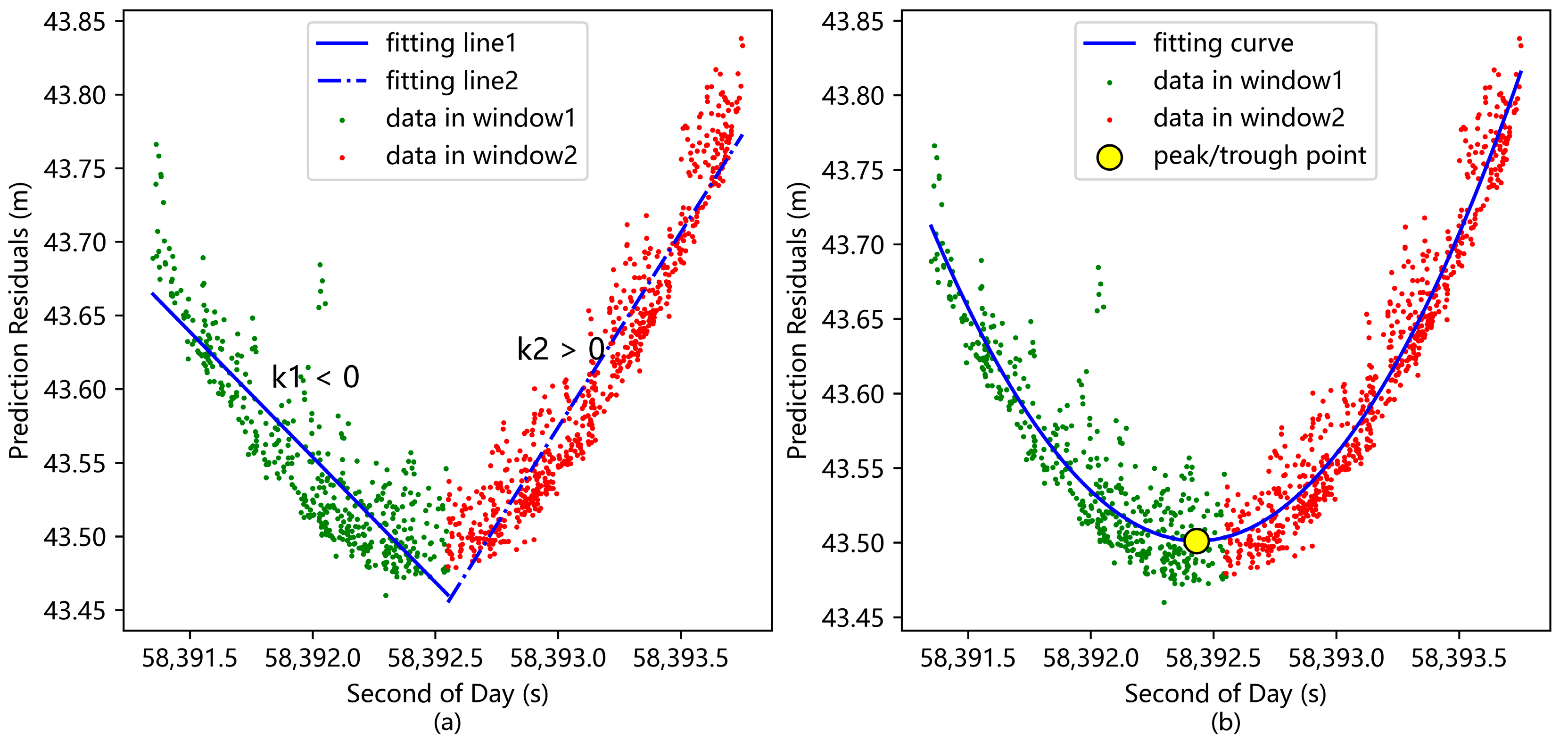
(1) Roughly determine the region of the data peak or trough point. Apply a sliding window technique to the time axis of the prediction residual data, perform a linear fit on the data within the window, and calculate the slope. If the slopes k1 and k2 obtained by fitting the data in two adjacent windows have opposite signs, i.e., the slopes change from positive to negative or from negative to positive, then it is considered that there is a peak or trough point within the two windows, as shown in Figure 3a.
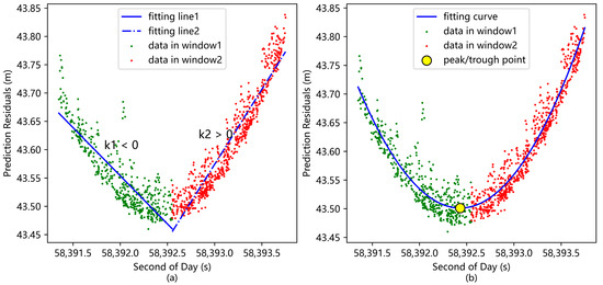
Figure 3.
Identification of peak or trough point in the prediction residual data. (a) Rough determination of the region of the data peak or trough point; (b) Precise estimation of the position of the data peak or trough point.
The detailed steps for solving k1 and k2 are as follows: Let the linear fitting function be , then the sum of the squares of the errors is . is at a minimum when is satisfied, i.e., . Solving this system of equations yields k and b0, and performing the above computational procedure for the data in the adjacent windows yields k1 and k2, respectively.
(2) Precisely estimate the position of the data peak or trough point. Perform parabolic fitting on the data of the two windows determined in step (1). Calculate the vertex position of the parabola through the fitting parameters, and this vertex is identified as the peak or trough point of the prediction residual data, as shown in Figure 3b.
The detailed procedure for solving the position of the vertex of the parabola is as follows: Let the parabolic fit function be , then the sum of the squares of the errors is . is at a minimum when is satisfied, i.e., . Solving this system of equations yields b2, b1, and b0, and the location of the parabola vertex is .
Since the pattern of prediction residual data keeps changing with time, we segment the prediction residuals on the time axis. The time coordinates of the data-segmented points are calculated from the identified peaks and troughs as in Equation (1):
where m represents the total number of datasets segmented by the prediction residual data, i denotes the index of the current dataset, n is the total number of peaks and troughs in a single dataset, j is the index of the segmentation point in a single dataset, is the time coordinate of the j-th segmentation point in dataset i, and is the time coordinate of the j-th peak or trough point in dataset i.
2.1.2. Determination of the Optimal Trend Function for Each Subinterval
The core of the noise rejection method proposed in this paper is to find a trend function that can accurately describe the variation pattern of the prediction residual data, and the data far from the curve of this function are regarded as noise and filtered out. Root mean squared error (RMSE) quantifies the agreement between the fitted function and the actual data, and the smaller the RMSE value is, the more accurate the fitted trend function is.
where represents the actual value, is the predicted value, and N is the total number of data points. From Equation (2), when the number of data points is fixed, the smaller the sum of squares of the difference between the actual value and the predicted value, the smaller the RMSE. Since the goal of the least squares method is to find the best function match for the data by minimizing the sum of squares of the differences between the actual and predicted values, it aligns with the current need to find the optimal trend function. Therefore, in this paper, the least squares polynomial fitting method is used to obtain the optimal trend function for each subinterval data in order to achieve the fit of the best trend function over the global data range. The sum of squares of the difference between the actual and predicted values is given by the following:
When Equation (3) satisfies the system of equations in Equation (4), reaches its minimum value.
The matrix form of Equation (4) can be expressed as follows:
In Equation (5), the matrix with respect to is a k + 1 dimensional square matrix, thus we can obtain Equation (6), and solve for the coefficients of the fitting polynomial.
2.1.3. Smooth Transition of Trend Functions Between Adjacent Subintervals
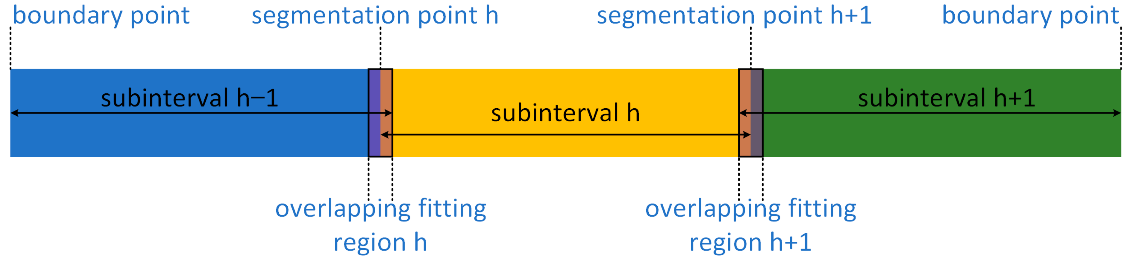
In this paper, the trend function of each subinterval is fitted independently, and no constraint is established between the trend functions of adjacent subintervals. Consequently, the transition at the junction of subintervals is discontinuous, and there exists a small numerical deviation. To address this issue, the paper proposes a scheme for smoothly transitioning the trend functions between adjacent subintervals. This scheme introduces an overlapping fitting region near the junction of two adjacent subintervals, as shown in Figure 4, and the steps to implement this scheme are as follows:
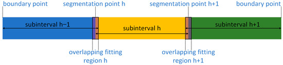
Figure 4.
Schematic of overlapping fitting regions.
- (1)
- Divide the data into multiple subintervals with overlapping parts.
- (2)
- Fit the data within each subinterval independently.
- (3)
- Combine the fitting results of adjacent subintervals within the overlapping region by means of a weight function.
In mathematics, assuming that the fitting functions for subintervals h and h + 1 are and , respectively. And the fitting result in the overlapping fitting region h + 1 can be expressed as follows:
where w1 and w2 are the weight functions of and , respectively.
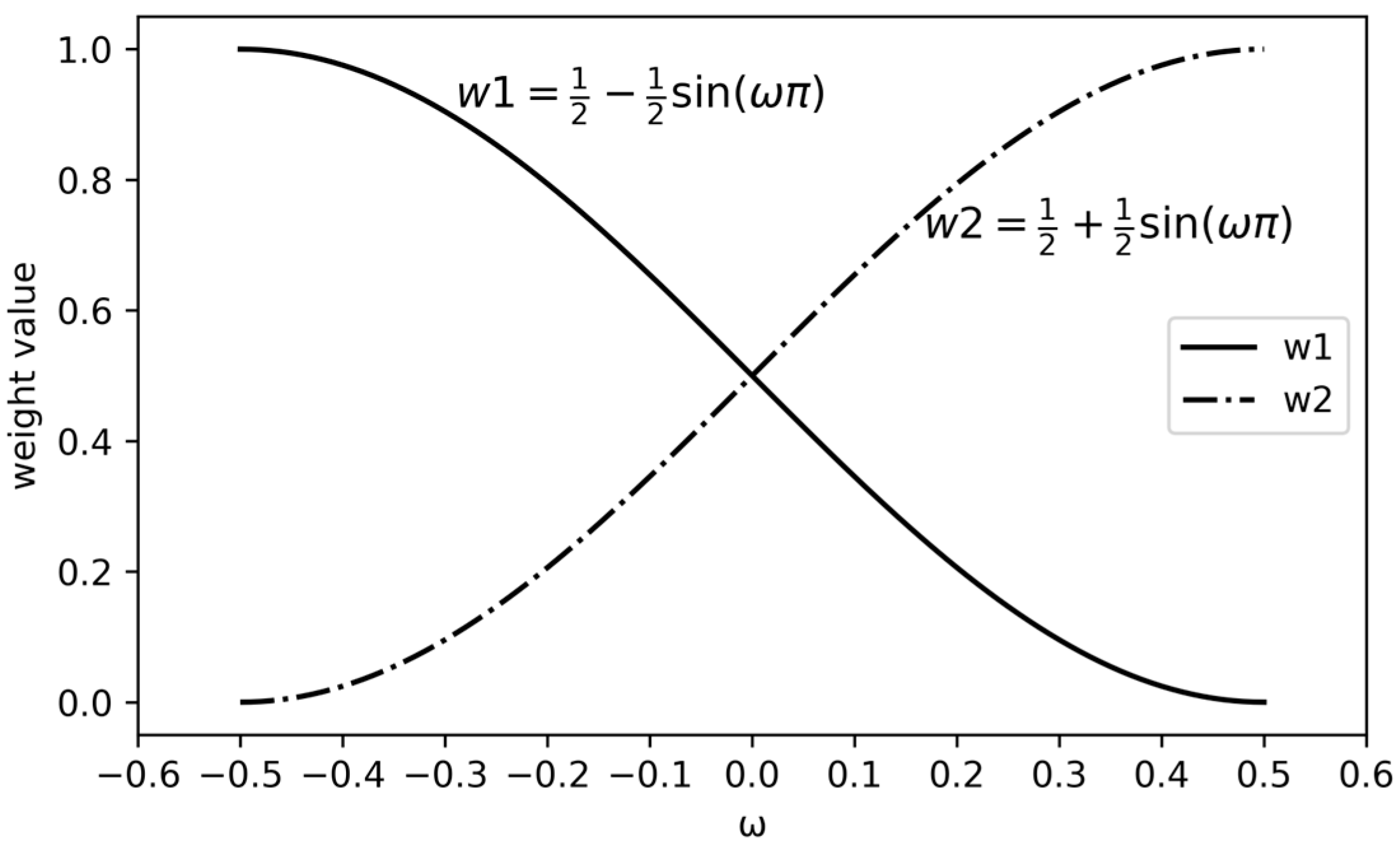
The weight functions w1 and w2 constructed in this paper for the overlapping region based on the characteristics of prediction residual data are shown in Equation (8), and the function curves are shown in Figure 5.
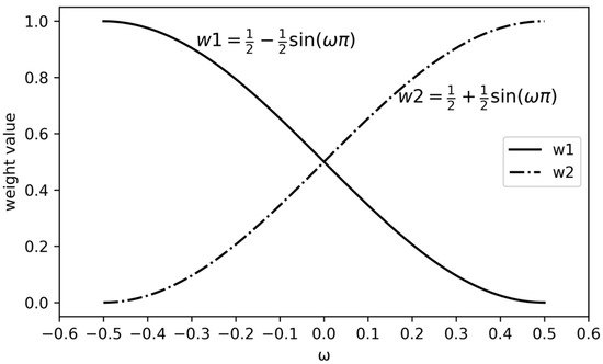
Figure 5.
Function curve of weights w1 and w2.
The weighting functions showed in Figure 5 have the following main properties:
- a.
- Smoothness: Both functions are constructed based on sinusoidal function, ensuring good continuity and derivability.
- b.
- Symmetry: The two functions are symmetric about w = 1/2.
- c.
- Complementarity: Both functions have a value range of [0, 1] and their sum is constant at 1.
- d.
- Normalization: The two functions complement each other; when one function decreases from 1 to 0, the other increases from 0 to 1.
This weight functions allow w1 to decrease from 1 to 0 and w2 to increase from 0 to 1, with w1 + w2 ≡ 1, thus realizing a smooth transition of the trend function from to in adjacent subintervals.
2.1.4. Filtering of Noise Data
The prediction residual of effective laser ranging data is a data band with a concentrated distribution, and the further away from the center of the data band, the lower the density of the data and the higher the noise probability. The prediction residual trend function curve obtained through the above process can be regarded as a theoretical curve aligned with the center of the prediction residual data band. The further away the prediction residual data is from the trend function curve, the greater the probability that it is noise. The difference between the prediction residual data and the trend function is referred to as the fit residual (denoted as FR), and the magnitude of the fit residual reflects the degree to which the data are off-center, and noise is identified and rejected by analyzing the fit residuals.
Root mean square (RMS) is a comprehensive index that measures the deviation between the data points and the zero value, especially when the data contain positive and negative values. The RMS can effectively synthesize the magnitude of these values to avoid positive and negative cancellation. In this study, the RMS value reflects the degree of dispersion of the data distribution and can further indicate the consistency between the fitting trend function and the data variation pattern. A smaller RMS value suggests that the distribution of the remaining data after noise removal is more concentrated, which also proves that the fitting trend function has a higher consistency with the data variation pattern. Conversely, it indicates that the fitting trend function has poorer consistency with the data variation pattern or is even completely different from the data variation pattern.
As in Equation (9), the RMS of the fit residuals is calculated, and when the absolute value of a fit residual value exceeds a certain threshold, the data corresponding to the fit residual is judged to be noise data and is eliminated.
where β is the scaling factor, which usually takes the value of 2.5 for single-photon detector [42], but not uniquely. By this method, we can effectively remove the noise from the laser ranging data and improve the accuracy and reliability of the data.
2.2. Laser Ranging Data Preprocessing Flow Based on Novel Spline Fitting
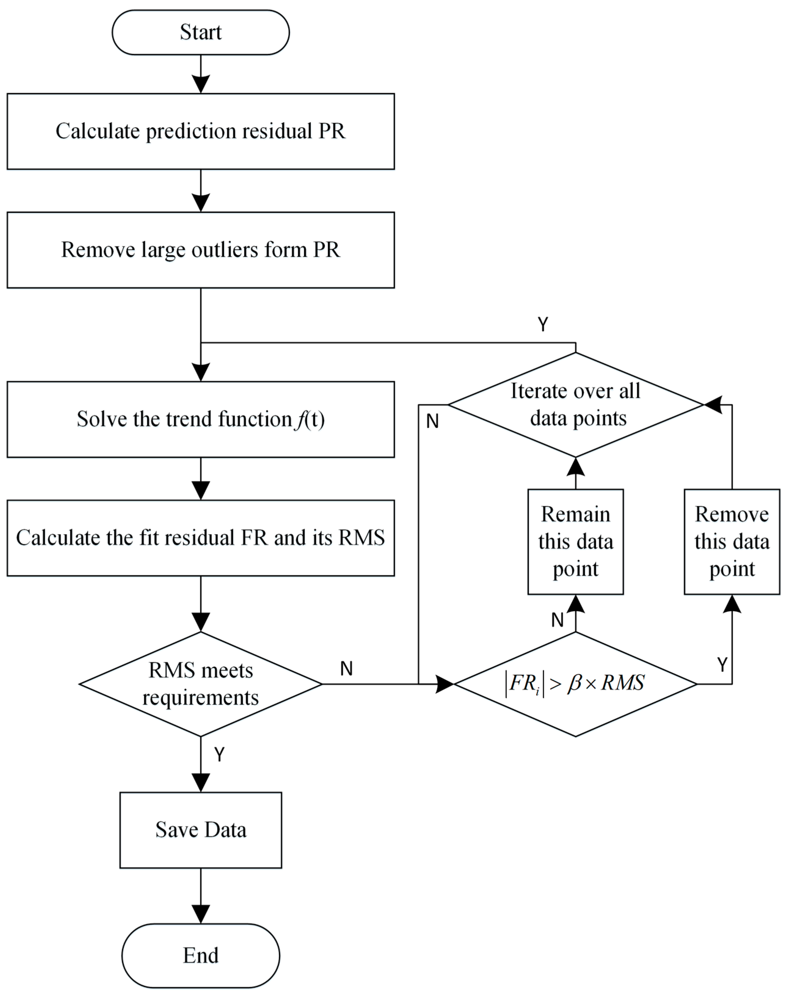
As shown in Figure 6, the laser ranging data preprocessing flow [47,48] based on novel spline fitting includes the following steps:
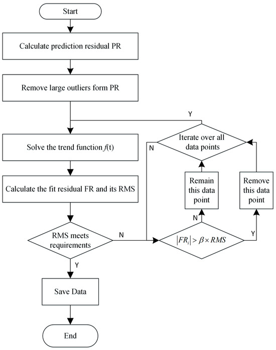
Figure 6.
Laser ranging data preprocessing flow based on novel spline fitting.
- (1)
- Calculate the prediction residual PR, i.e., the difference between the observed value O and the computed value C (Observed-Computed), using high-precision prediction and measured data;
- (2)
- Remove outliers from the prediction residual PR by manual or automatic data identification techniques;
- (3)
- Solve the trend function f(t) of the prediction residuals using a novel spline fitting method;
- (4)
- Calculate the fit residual FR, i.e., the difference between PR and f(t), and solve the RMS of the fit residual;
- (5)
- Identify the noise by setting the threshold window β × RMS, remove the noise data outside the threshold window, and use the remaining data for the next iteration;
- (6)
- Repeat steps (3) to (5) until the RMS meets the preset requirements and save the preprocessed data.
3. Results
In order to test the effectiveness and applicability of the laser ranging data preprocessing method proposed in this paper, we selected the corresponding data samples based on different data characteristics such as signal-to-noise ratio, fluctuation amplitude, frequency, and continuity. Then, the traditional preprocessing method based on polynomial fitting and the preprocessing method based on novel spline fitting were applied to preprocess these data, respectively. In order to comprehensively assess the effectiveness of the methods, validation experiments calculated the RMS values of the fit residuals of each preprocessing method before and after noise rejection and compared the results before and after preprocessing, as well as the comparison between the two different methods. The laser ranging data used in this paper are all actual measured data from the Changchun Station (7237).
3.1. Preprocessing of Data with Good Characteristics
To simplify case comparisons, we selected a sample that performs well in all aspects of data characterization, as shown in Figure 7, where we selected the Topex (22076) measured data acquired on 25 June 2024 at 16:00 UTC. As can be seen from the figure, the selected data have a high signal-to-noise ratio, small amplitude variation, moderate frequency, and good continuity.
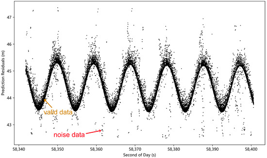
Figure 7.
Prediction residuals of Topex measured data with residual noise.
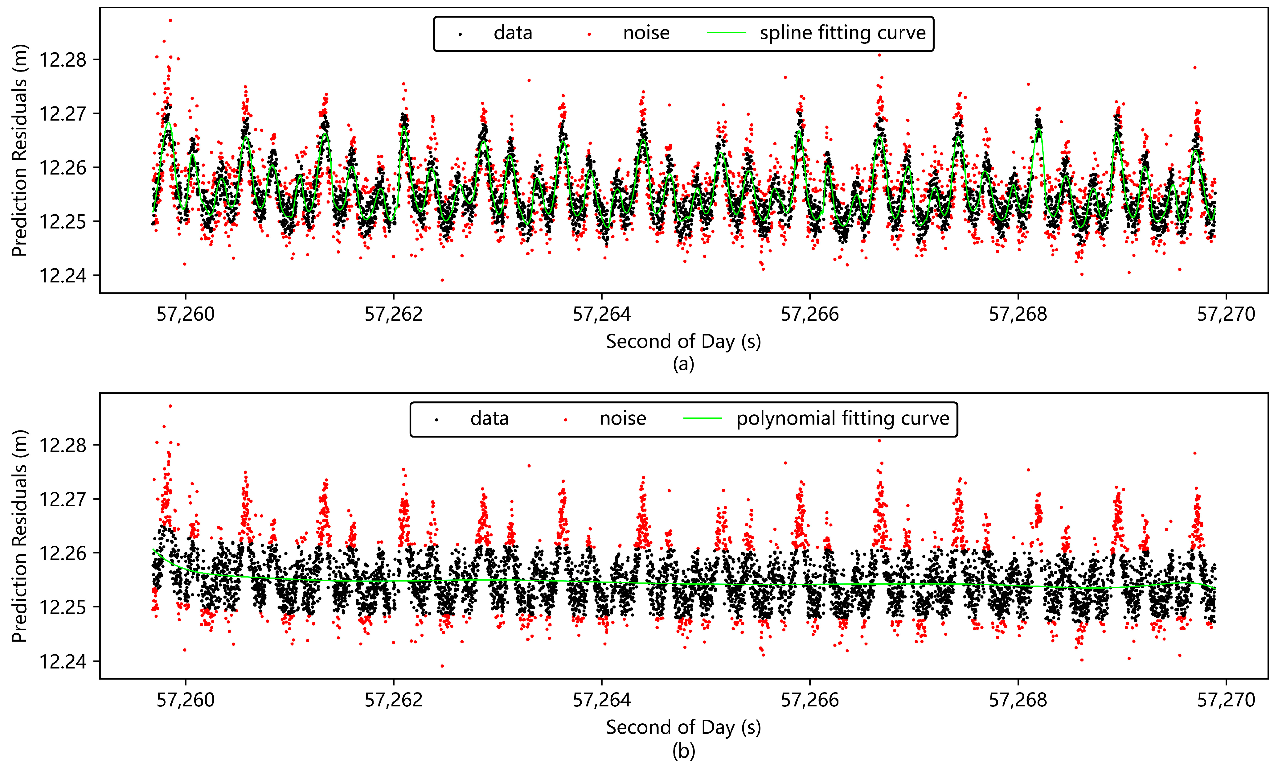
Figure 8 demonstrates the preprocessing results of the prediction residuals for the same set of laser ranging data using two different preprocessing methods. From the figure, it can be observed that the trend function obtained by the novel spline fitting method coincides with the variation trend of the data, successfully filtering out the residual noise away from the data band while retaining the original pattern of the data. In contrast, the trend function calculated by the polynomial fitting method does not match the variation trend of the data, and there is still a large amount of residual noise after the preprocessing, and some of the valid data with peaks and troughs are mistakenly deleted. The data in Table 1 also show that the RMS value of the novel spline fitting method after noise removal is one-fourth of that before noise removal and only one-seventh of that after noise removal of the polynomial fitting method, and the data accuracy is significantly improved. Through the above analysis and comparison, the preprocessing effect of the novel spline fitting method is significantly better than that of the polynomial fitting method when dealing with data with good characteristics.
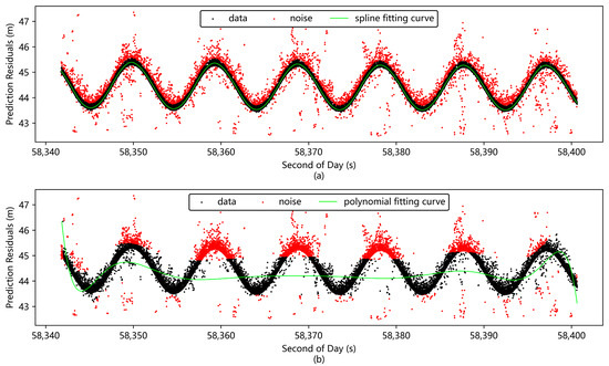
Figure 8.
Preprocessing results for data with good characteristics. (a) Preprocessing results of the novel spline fitting method; (b) Preprocessing result of the polynomial fitting method.

Table 1.
Preprocessing results for data with good characteristics.
3.2. Preprocessing of Low Signal-to-Noise Ratio Data
To investigate the effect of data preprocessing in the case of a low signal-to-noise (S/N) ratio, we selected the Topex (22076) measured data on 28 April 2016 at 6:00 UTC as the experimental sample. As shown in Figure 9, the prediction residuals of these data exhibit the characteristics of a low S/N ratio, with the valid data vaguely discernible and strongly disturbed by noise.
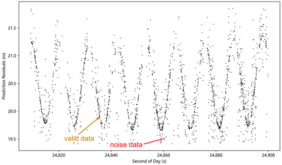
Figure 9.
Prediction residuals of Topex measured data characterized by low S/N ratio.
From Figure 10 and Table 2, it can be found that the preprocessing results of the two methods for low S/N ratio data are similar to those for good characteristic data discussed in Section 3.1. However, the data with low S/N ratio are usually generated under poor observational conditions, and the use of the new spline fitting method to filter out noise from such data and extract high-precision information is crucial for increasing the sample size of valid data under poor observational conditions. The comparison results highlight the significant advantages of the novel spline method in processing low S/N ratio data.
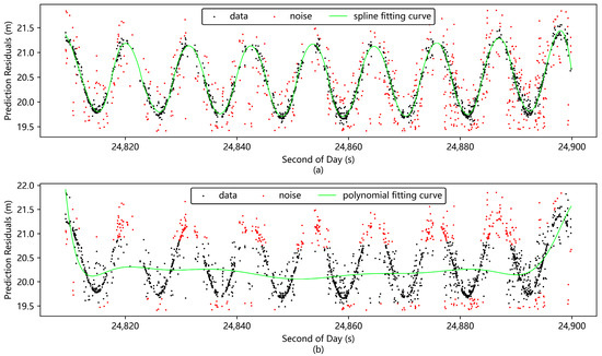
Figure 10.
Preprocessing results for data with low S/N ratio. (a) Preprocessing results of the novel spline fitting method; (b) Preprocessing result of the polynomial fitting method.
Table 2.
Preprocessing results for data with low S/N ratio.
3.3. Preprocessing of High-Frequency Fluctuation Data
In this experiment, we selected the Ajisai (16908) measured data at 15:00 UTC on 13 July 2015 as a representative sample of high-frequency fluctuation data. As shown in Figure 11, the prediction residuals of the Ajisai data exhibit the characteristics of high frequency and small amplitude, and the noise interspersed within the data makes it difficult to distinguish the peak and trough characteristics.
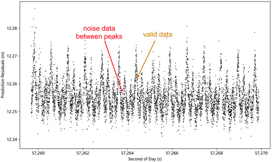
Figure 11.
Prediction residuals data of Ajisai characterized by high-frequency fluctuations.
Figure 12 shows the preprocessing results of two different methods for high-frequency fluctuation data. The novel spline fitting method can effectively filter out the noise data between the peaks and troughs, which not only improves the accuracy of the data, but also enhances the clarity of the peaks and troughs features of the data, and provides an accuracy guarantee for analyzing the target motion state with high precision. In contrast, the polynomial fitting method obviously deletes the valid data with peak and trough characteristics by mistake in the process, which not only reduces the recognizability of the data features but also destroys the original pattern of the data. Despite the small amplitude and high concentration of prediction residual data, and the RMS values after preprocessing of both methods are not large, the RMS value of the novel spline fitting method is still only about one-half of the RMS of the polynomial fitting method after preprocessing, as shown in Table 3. These results indicate that the novel spline fitting method is more effective in dealing with high-frequency fluctuation data.
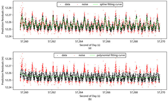
Figure 12.
Preprocessing results for data with high-frequency fluctuation. (a) Preprocessing results of the novel spline fitting method; (b) Preprocessing result of the polynomial fitting method.
Table 3.
Preprocessing results for data with high-frequency fluctuation.
3.4. Preprocessing of Data with Amplitude Variation Characteristics
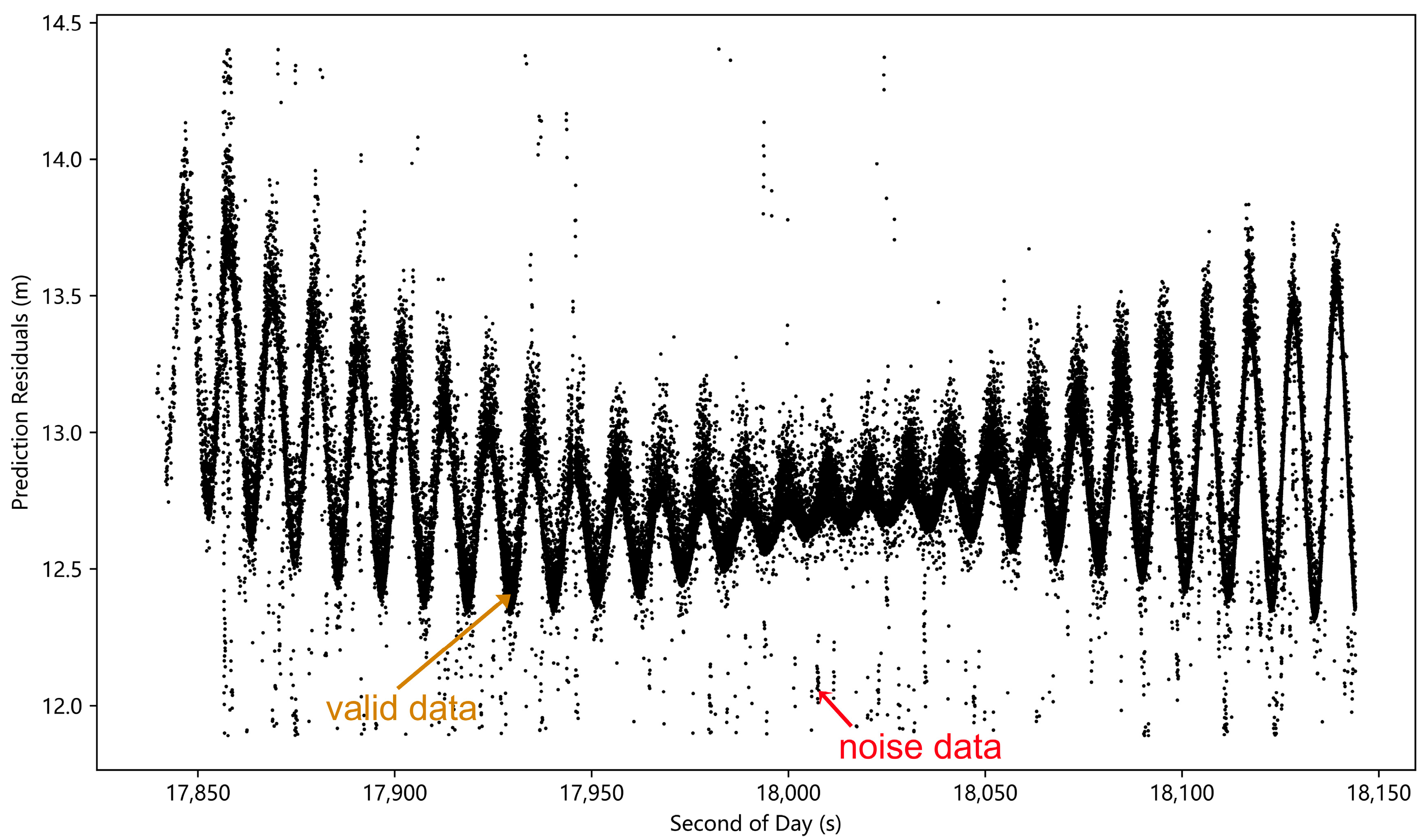
In this experiment, we selected the Topex (22076) measured data at 4:00 UTC on 28 April 2016 as a sample, which has obvious characteristics of amplitude variation. As shown in Figure 13, the prediction residuals still contain a large amount of residual noise after the automatic identification of valid data, and the amplitude shows a fluctuation characteristic of first decreasing and then increasing.

Figure 13.
Prediction residuals from Topex measured data characterized by amplitude variation.
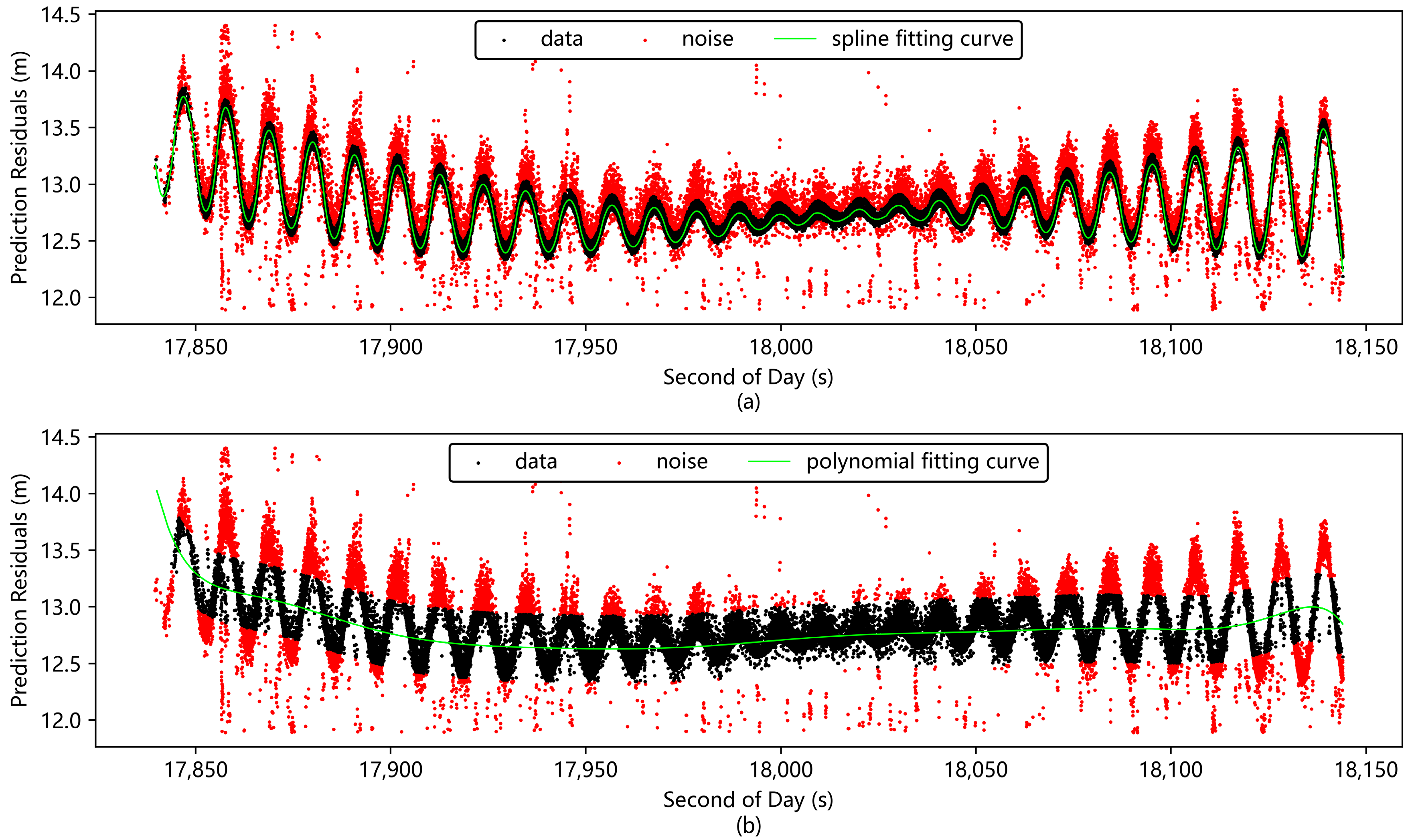
From the data preprocessing results in Figure 14, the trend function calculated by the novel spline fitting method changes adaptively with the fluctuation of data amplitude, effectively filtering out the residual noise while retaining the original variation pattern of the data. However, after the preprocessing of the polynomial fitting method, there is still a significant amount of noise near the data band, and several effective data constituting the peaks and troughs are mistakenly deleted, which destroys the original pattern of the data. As shown in Table 4, the RMS value after preprocessing of the novel spline fitting method is about one-fifth of the polynomial fitting method, and the data accuracy is higher. These results demonstrate the excellent ability of the novel spline fitting method in processing data with amplitude variation.
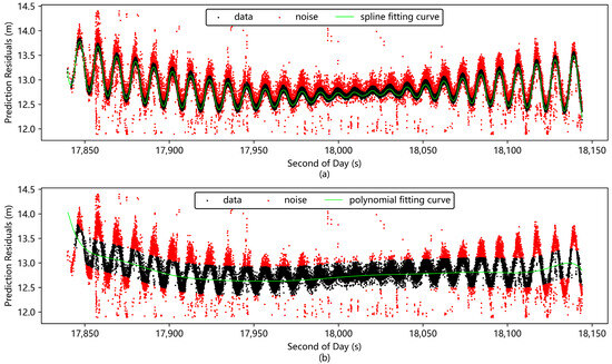
Figure 14.
Preprocessing results for data with amplitude variation. (a) Preprocessing results of the novel spline fitting method; (b) Preprocessing result of the polynomial fitting method.
Table 4.
Preprocessing results for data with amplitude variation.
3.5. Preprocessing of Discontinuous Data
The measured data of Topex (22076) at 14:00 UTC on 25 June 2024 is selected as a sample for this experiment, which consists of several discontinuous arc segments with residual noise mixed in each arc segment, as shown in Figure 15.
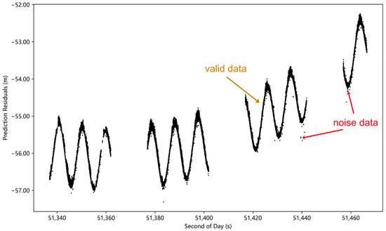
Figure 15.
Prediction residuals of Topex measured data with discontinuous feature.
The preprocessing results of the novel spline fitting method and polynomial fitting method are shown in Figure 16. From Figure 16a, it can be seen that the novel spline fitting method can automatically identify the break points of continuous data and accordingly divide the sub-datasets. Independent spline fitting is performed on each sub-dataset, resulting in a trend function that is highly consistent with the data’s variation trend. This method effectively filters out residual noise while retaining the complete information of the data. While the traditional polynomial fitting method deals with the data in the global scope, its calculated trend function is less consistent with the variation pattern of the data, residual noise still exists after preprocessing, and some effective data are deleted by mistake. As shown in Table 5, the RMS value of the novel spline fitting method after noise removal is only one-eighteenth of the polynomial fitting method, and the preprocessing effect is greatly better than that of the polynomial fitting method. The comparison results show that the novel spline fitting method has great advantages in processing discontinuous data and can improve the data quality significantly.
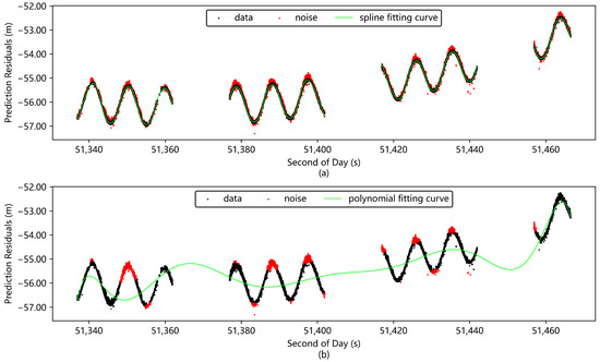
Figure 16.
Preprocessing results for discontinuous data. (a) Preprocessing results of the novel spline fitting method; (b) Preprocessing result of the polynomial fitting method.
Table 5.
Preprocessing results for discontinuous data.
4. Discussion
To verify the proposed method’s effectiveness and wide applicability, this study carefully selects data samples for experimentation based on the characteristics of frequency, amplitude, signal-to-noise ratio, and continuity. To facilitate comparison and analysis, we summarize the results of each validation experiment in Table 6.
Table 6.
Summary of results of method validation experiments.
By comparing and analyzing the resultant data before and after preprocessing, it can be seen that both methods successfully reduced the RMS values of the fit residuals. It is particularly noteworthy that the RMS value after preprocessing of the novel spline fitting method is much smaller than that of the polynomial fitting method, indicating that the preprocessed data of this method is more centralized and more accurate. According to the item “Mistaken Deletion of Valid Data”, the polynomial fitting method has mistakenly deleted valid data in all the validation experiments, which destroys the integrity of the true motion patterns carried by the data and negatively affects the subsequent data analysis and application instead of benefiting them. On the contrary, the novel spline fitting method successfully maintains the integrity of the original data patterns during the data preprocessing process while eliminating noise and improving the data accuracy, further confirming the effectiveness of the method. The novel spline fitting method has achieved excellent results in data preprocessing for all types of features, fully demonstrating the robustness and general applicability of the method. During the research process, we found that in the preprocessing process of laser ranging data, solving the trend function matching the data pattern is crucial, which directly determines the availability and accuracy of the preprocessed data, which in turn has an impact on the further analysis and application of the data. With the application of a higher frequency laser ranging system, the amount of mineable information carried in the laser ranging data will continue to increase, and at the same time, the various interferences contained in the data will also be more complex. How to effectively filter out the various interferences and retain the effective data will continue to be a hot topic of research in the future.
In terms of execution efficiency, theoretically, the novel spline fitting method shares the common problem of all algorithms, i.e., computational efficiency is affected by data volume, while in the process of practical application, its execution efficiency is comparable to that of the polynomial fitting method, which can fully meet the demand of engineering applications, and it has been applied to the daily data processing work of Changchun station.
In addition, a discussion on the applicability of the novel spline method in real-time space debris monitoring is presented here. Space debris is affected by various factors, such as Earth’s gravity and solar pressure, which lead to real-time changes in its state of motion, so real-time monitoring of space debris is of great significance. In the research process, it was found that the novel spline method is potentially applicable to the real-time monitoring of space debris. The method can automatically identify the peaks and troughs of the data and carry out segmented processing and segmented data fitting. The processing of segmented data reduces the computational complexity. And the latest segmented fitting function obtained in real time can be connected with the existing fitting function during the monitoring process, resulting in a real-time growing function curve, so as to realize the application of the novel spline method in space debris monitoring. The variation pattern of the fitting function can be analyzed in the monitoring process to quickly determine the motion state of the measured target, providing data reference for tasks such as space debris collision warning and avoidance. At the same time, there are some limitations. The novel spline method is to solve the trend function that coincides with the data variation, and if there are no valid data or the valid data are very weak in the process of space debris monitoring, the trend function obtained by the novel spline method will have a large error. Therefore, more in-depth analyses and research are needed in this area.
5. Conclusions
Addressing the challenges of the traditional polynomial fitting method in processing space target laser ranging data with complex characteristics, such as low data preprocessing accuracy, the ease of mistakenly deleting valid data, and damage to the target’s motion state information, as well as the current situation in which the traditional spline function fails to satisfy the preprocessing needs of laser ranging data, a novel spline function is constructed innovatively in this paper, and a laser ranging data preprocessing method is proposed based on this function. The method is able to adapt to data variation, automatically identify the peaks, troughs, and data breaks in the prediction residual data, reasonably segment the data based on these key feature points, and optimally fit the data in each segment to obtain the segment fitting function. Finally, by using a concatenation function, each segmented function is smoothly connected to form a spline function that adapts to the trend of data variation. And then the spline function is used for data filtering to effectively eliminate noise.
The preprocessing capability of the traditional method and the novel spline fitting method is validated using the observation data with different characteristics provided by Changchun station (7237). The results clearly show that the proposed method in this paper effectively removes the noise and significantly improves the data accuracy while successfully retaining the original pattern of the data. The RMS of the novel spline fitting method is about one-fourth of the RMS before noise removal, and the minimum is only one-eighteenth of the RMS of the traditional method. Moreover, as the number of noise removal iterations increases, the RMS value further decreases, and the data accuracy will be further improved. In contrast, the traditional method still leaves a large amount of noise after noise removal and is prone to mistakenly deleting key feature data, which destroys the target information contained in the data. This study provides a novel, efficient, and reliable preprocessing scheme for processing complex laser ranging data and verifying its effectiveness and general applicability. This method is an important supplement to the existing SLR data preprocessing methods, which is not only of great significance and value for the motion state analysis and high-precision orbiting of space targets but can also be extended to other potential applications, such as orbital analysis, space debris monitoring and collision warning, and lunar laser ranging data processing.
Author Contributions
Conceptualization, Y.Z., X.D., X.H. and Z.L.; methodology, Y.Z., X.D., X.H. and Z.L.; software, Y.Z. and Z.L.; validation, Y.Z., X.D. and Z.L.; formal analysis, Y.Z., X.D., X.H. and Z.L.; investigation, J.G. and Y.L.; resources, X.H. and X.D.; data curation, Q.S.; writing—original draft preparation, Y.Z.; writing—review and editing, Y.Z., X.D., H.D. and X.H.; visualization, Y.Z.; supervision, X.D. and X.H.; funding acquisition, H.D. and J.G. All authors have read and agreed to the published version of the manuscript.
Funding
This research was funded by Natural Science Foundation of Jilin Province (grant number 20220101125JC), and the National Natural Science Foundation of China (grant number 12273079).
Data Availability Statement
The data presented in this study are available upon request from the corresponding author. The data are not publicly available due to privacy.
Acknowledgments
The laser ranging data are provided by Changchun Observatory, National Astronomical Observatories, Chinese Academy of Sciences.
Conflicts of Interest
The authors declare no conflicts of interest.
Abbreviations
The following abbreviations are used in this manuscript:
| SLR | Satellite laser ranging |
| ILRS | International Laser Ranging Service |
| EOP | Earth orientation parameters |
| RMSE | Root mean squared error |
References
- Pearlman, M.; Arnold, D.; Davis, M.; Barlier, F.; Biancale, R.; Vasiliev, V.; Ciufolini, I.; Paolozzi, A.; Pavlis, E.C.; Sośnica, K.; et al. Laser Geodetic Satellites: A High-Accuracy Scientific Tool. J. Geod. 2019, 93, 2181–2194. [Google Scholar] [CrossRef]
- Sośnica, K.; Bury, G.; Zajdel, R. Contribution of Multi-GNSS Constellation to SLR-Derived Terrestrial Reference Frame. Geophys. Res. Lett. 2018, 45, 2339–2348. [Google Scholar] [CrossRef]
- Maier, A.; Krauss, S.; Hausleitner, W.; Baur, O. Contribution of Satellite Laser Ranging to Combined Gravity Field Models. Adv. Space Res. 2012, 49, 556–565. [Google Scholar] [CrossRef]
- Lemoine, F.G. The Contribuons of Satellite Laser Ranging to Satellite Altimetry. In Proceedings of the 20th International Workshop on Laser Ranging, Potsdam, Germany, 9–14 October 2016; p. 40. [Google Scholar]
- Kirchner, G.; Koidl, F. Graz kHz SLR System: Design, Experiences and Results. Available online: https://ilrs.cddis.eosdis.nasa.gov/lw14/docs/papers/adv4_gkm.pdf (accessed on 12 January 2025).
- Wu, Z.; Zhang, H.; Zhang, Z.; Yang, F.; Chen, J.; Li, P. kHz repetition Satellite Laser Ranging system with high precision and measuring results. Chin. Sci. Bull. 2011, 56, 1177–1183. [Google Scholar] [CrossRef]
- Gibbs, P.; Potter, C.; Sherwood, R.; Wilkinson, M.; Benham, D.; Smith, V.; Appleby, G. Some Early Results of Kilohertz Laser Ranging at Herstmonceux. Available online: https://ilrs.gsfc.nasa.gov/lw15/docs/papers/Some%20Early%20Results%20of%20Kilohertz%20Laser%20Ranging%20at%20Herstmonceux.pdf (accessed on 6 January 2025).
- Fan, Z.; Liu, X.; Zhang, Z.; Meng, W.; Long, M.; Bai, Z. 10 kHz Repetition Rate Picosecond Green Laser for High-Accuracy Satellite Ranging. Front. Phys. 2023, 10, 1115330. [Google Scholar] [CrossRef]
- Cheng, S.; Long, M.; Zhang, H.; Wu, Z.; Qin, S.; Zhang, Z. Research on satellite laser ranging at pulse repetition frequency of 100 kHz. Infrared Laser Eng. 2022, 51, 20220121. [Google Scholar] [CrossRef]
- Hampf, D.; Wagner, P.; Schafer, E.; Riede, W. Concept for a New Minimal SLR System. Available online: https://ilrs.gsfc.nasa.gov/lw21/docs/2018/papers/Session8_Hampf_Paper.pdf (accessed on 21 January 2025).
- Courde, C.; Mariey, H.; Chabé, J.; Phung, D.-H.; Torre, J.-M.; Aimar, M.; Maurice, N.; Samain, E.; Tosi, A.; Buttafava, M. High Repetition Rate SLR at GRSM. Available online: https://ilrs.gsfc.nasa.gov/2019_Technical_Workshop/docs/2019/abstracts/session4_Courde_abstract.pdf (accessed on 19 January 2025).
- Wang, P.; Steindorfer, M.A.; Koidl, F.; Kirchner, G.; Leitgeb, E. Megahertz Repetition Rate Satellite Laser Ranging Demonstration at Graz Observatory. Opt. Lett. 2021, 46, 937–940. [Google Scholar] [CrossRef] [PubMed]
- Wilkinson, M.; Schreiber, U.; Procházka, I.; Moore, C.; Degnan, J.; Kirchner, G.; Zhongping, Z.; Dunn, P.; Shargorodskiy, V.; Sadovnikov, M.; et al. The next Generation of Satellite Laser Ranging Systems. J. Geod. 2019, 93, 2227–2247. [Google Scholar] [CrossRef]
- Tang, R.; Li, Y.; Li, X.; Li, R.; Huang, K. Spin Rate Determination of AJISAI Based on High Frequency Satellite Laser Ranging. Chin. J. Lasers 2015, 42, 287–292. [Google Scholar]
- Liu, T.; Chen, H.; Shen, M.; Gao, P.; Zhao, Y. Spinning Satellite Laser Ranging Data Analysis and Processing. Chin. J. Lasers 2017, 44, 0504001. [Google Scholar] [CrossRef]
- Kucharski, D.; Kirchner, G.; Otsubo, T.; Lim, H.-C.; Bennett, J.; Koidl, F.; Kim, Y.-R.; Hwang, J.-Y. Confirmation of Gravitationally Induced Attitude Drift of Spinning Satellite Ajisai with Graz High Repetition Rate SLR Data. Adv. Space Res. 2016, 57, 983–990. [Google Scholar] [CrossRef]
- Kessler, D.J.; Cour-Palais, B.G. Collision Frequency of Artificial Satellites: The Creation of a Debris Belt. J. Geophys. Res. Space Phys. 1978, 83, 2637–2646. [Google Scholar] [CrossRef]
- Liou, J.-C.; Johnson, N.L. Risks in Space from Orbiting Debris. Science 2006, 311, 340–341. [Google Scholar] [CrossRef]
- Krag, H.; Serrano, M.; Braun, V.; Kuchynka, P.; Catania, M.; Siminski, J.; Schimmerohn, M.; Marc, X.; Kuijper, D.; Shurmer, I.; et al. A 1 Cm Space Debris Impact onto the Sentinel-1A Solar Array. Acta Astronaut. 2017, 137, 434–443. [Google Scholar] [CrossRef]
- Kirchner, G.; Koidl, F.; Friederich, F.; Buske, I.; Völker, U.; Riede, W. Laser Measurements to Space Debris from Graz SLR Station. Adv. Space Res. 2013, 51, 21–24. [Google Scholar] [CrossRef]
- Liang, Z.; Dong, X.; Ibrahim, M.; Song, Q.; Han, X.; Liu, C.; Zhang, H.; Zhao, G. Tracking the Space Debris from the Changchun Observatory. Astrophys. Space Sci. 2019, 364, 201. [Google Scholar] [CrossRef]
- Steindorfer, M.A.; Kirchner, G.; Koidl, F.; Wang, P.; Jilete, B.; Flohrer, T. Daylight Space Debris Laser Ranging. Nat. Commun. 2020, 11, 3735. [Google Scholar] [CrossRef]
- Smagło, A.; Lejba, P.; Schillak, S.; Suchodolski, T.; Michałek, P.; Zapaśnik, S.; Bartoszak, J. Measurements to Space Debris in 2016–2020 by Laser Sensor at Borowiec Poland. Artif. Satell. 2021, 56, 119–134. [Google Scholar] [CrossRef]
- Kucharski, D.; Kirchner, G.; Koidl, F.; Fan, C.; Carman, R.; Moore, C.; Dmytrotsa, A.; Ploner, M.; Bianco, G.; Medvedskij, M.; et al. Attitude and Spin Period of Space Debris Envisat Measured by Satellite Laser Ranging. IEEE Trans. Geosci. Remote Sens. 2014, 52, 7651–7657. [Google Scholar] [CrossRef]
- Kirchner, G.; Kucharski, D.; Cristea, E. Gravity Probe-B: New Methods to Determine Spin Parameters from kHz SLR Data. IEEE Trans. Geosci. Remote Sens. 2009, 47, 370–375. [Google Scholar] [CrossRef]
- Kucharski, D.; Kirchner, G.; Bennett, J.C.; Lachut, M.; Sośnica, K.; Koshkin, N.; Shakun, L.; Koidl, F.; Steindorfer, M.; Wang, P.; et al. Photon Pressure Force on Space Debris TOPEX/Poseidon Measured by Satellite Laser Ranging. Earth Space Sci. 2017, 4, 661–668. [Google Scholar] [CrossRef]
- Liu, T.; Shen, M.; Gao, P.; Zhao, Y. Tumbling Motion Estimation of Rocket Body Based on Diffuse Reflection Laser Ranging. Chin. J. Lasers 2019, 46, 0104007. [Google Scholar] [CrossRef]
- Guo, J.; Wang, Y.; Shen, Y.; Liu, X.; Sun, Y.; Kong, Q. Estimation of SLR Station Coordinates by Means of SLR Measurements to Kinematic Orbit of LEO Satellites. Earth Planets Space 2018, 70, 201. [Google Scholar] [CrossRef]
- Rutkowska, M.; Jagoda, M. SLR Technique Used for Description of The Earth Elasticity. Artif. Satell. 2015, 50, 127–141. [Google Scholar] [CrossRef]
- Tang, R.; Zhai, D.; Zhang, H.; Pi, X.; Li, C.; Fu, H.; Li, R.; Li, Z.; Li, Y. Research Progress in Space Debris Laser Ranging. Space Debris Res. 2020, 20, 21–30. [Google Scholar]
- Greene, B. Laser Tracking of Space Debris. Available online: https://ilrs.cddis.eosdis.nasa.gov/lw13/docs/papers/adv_greene_1m.pdf (accessed on 26 January 2025).
- Kucharski, D.; Kirchner, G.; Jah, M.K.; Bennett, J.C.; Koidl, F.; Steindorfer, M.A.; Wang, P. Full Attitude State Reconstruction of Tumbling Space Debris TOPEX/Poseidon via Light-Curve Inversion with Quanta Photogrammetry. Acta Astronaut. 2021, 187, 115–122. [Google Scholar] [CrossRef]
- Cordelli, E.; Mira, A.D.; Flohrer, T.; Setty, S.; Zayer, I.; Scharring, S.; Dreyer, H.; Wagner, G.; Kästel, J.; Schafer, E.; et al. Ground-Based Laser Momentum Transfer Concept for Debris Collision Avoidance. J. Space Saf. Eng. 2022, 9, 612–624. [Google Scholar] [CrossRef]
- Hall, A.; Steele, P.; Moulin, J.; Ferreira, E. Airbus Active Debris Removal Service. Adv. Astronaut. Sci. Technol. 2021, 4, 1–10. [Google Scholar] [CrossRef]
- Phipps, C.R.; Baker, K.L.; Libby, S.B.; Liedahl, D.A.; Olivier, S.S.; Pleasance, L.D.; Rubenchik, A.; Trebes, J.E.; Victor George, E.; Marcovici, B.; et al. Removing Orbital Debris with Lasers. Adv. Space Res. 2012, 49, 1283–1300. [Google Scholar] [CrossRef]
- Ibrahim, M.; Hanna, Y.S.; Samwel, S.W. Statistical and Comparative Studies for the Observations of Helwan-SLR Station. Int. J. Nonlinear Sci. Numer. Simul. 2004, 5, 135–148. [Google Scholar] [CrossRef]
- Kucharski, D.; Otsubo, T.; Kirchner, G.; Lim, H.-C. Spectral Filter for Signal Identification in the kHz SLR Measurements of the Fast Spinning Satellite Ajisai. Adv. Space Res. 2013, 52, 930–935. [Google Scholar] [CrossRef]
- Ma, T.; Zhao, C.; He, Z.; Zhang, H. Realtime recognition method of weak signal in space debris laser ranging. Acta Geod. Cartogr. Sin. 2022, 51, 87–94. [Google Scholar]
- Moore, C. Development of Automated SLR Data Processing at Mt Stromlo SLR Station. In Proceedings of the 21st International Workshop on Laser Ranging, Canberra, Australia, 5–9 November 2018; p. 22. [Google Scholar]
- Hiener, M.; Schreiber, U.; Brandl, N. Recursive Filter Algorithm for Noise Reduction in SLR. In Proceedings of the 15th International Workshop on Laser Ranging, Canberra, Australia, 15–20 October 2006; p. 6. [Google Scholar]
- Fang, Q.; Zhao, Y. The research progress in data processing algorithm of satellite laser ranging. Laser Technol. 2008, 32, 417–419. [Google Scholar]
- Li, Y.; Fu, H.; Li, R.; Tang, R.; Li, Z.; Zhai, D.; Zhang, H.; Pi, X.; Ye, X.; Xiong, Y. Research and Experiment of Lunar Laser Ranging in Yunnan Observatories. Chin. J. Lasers 2019, 46, 0104004. [Google Scholar] [CrossRef]
- Kucharski, D.; Kirchner, G.; Otsubo, T.; Koidl, F. A Method to Calculate Zero-Signature Satellite Laser Ranging Normal Points for Millimeter Geodesy—A Case Study with Ajisai. Earth Planets Space 2015, 67, 34. [Google Scholar] [CrossRef]
- Liu, J.; Zhang, G.; Feng, X.; Zhang, Z.; Li, S.; Hu, B. High Precision Centroid Location Algorithm Based on Cubic Spline Fitting and Interpolation. Acta Opt. Sin. 2021, 41, 1212004. [Google Scholar] [CrossRef]
- Tao, T. Stability Analysis and Application of Cubic Spline Interpolation Function; Chengdu University of Technology: Chengdu, China, 2023. [Google Scholar]
- Hu, J. Research of Dual-Wavelength Satellite Laser Ranging, Shanghai Astronomical Observatory; Chinese Academy of Sciences: Shanghai, China, 2003. [Google Scholar]
- Sinclair, A.T. Re-Statement of Herstmonceux Normal Point Recommendation. Available online: https://ilrs.gsfc.nasa.gov/data_and_products/data/npt/npt_algorithm.html (accessed on 24 December 2024).
- Torrence, M.H.; Klosko, S.M. The Construction and Testing of Normal Points at Goddard Space Flight Center; NASA: Washington, DC, USA, 1984; pp. 506–516. [Google Scholar]


Disclaimer/Publisher’s Note: The statements, opinions and data contained in all publications are solely those of the individual author(s) and contributor(s) and not of MDPI and/or the editor(s). MDPI and/or the editor(s) disclaim responsibility for any injury to people or property resulting from any ideas, methods, instructions or products referred to in the content. |
© 2025 by the authors. Licensee MDPI, Basel, Switzerland. This article is an open access article distributed under the terms and conditions of the Creative Commons Attribution (CC BY) license (https://creativecommons.org/licenses/by/4.0/).