
Adversarial Positive-Unlabeled Learning-Based Invasive Plant Detection in Alpine Wetland Using Jilin-1 and Sentinel-2 Imageries


Abstract
1. Introduction
- An APUL framework is designed for high-accuracy IP detection by utilizing only a limited number of labeled samples of the target species.
- An improved adversarial structure is proposed that utilizes a dual-branch discriminator to constrain the class prior-free classifier through the adversarial process.
- The proposed APUL approach was employed to map the detailed distribution of Pedicularis kansuensis in Bayinbuluk Grassland, and the experimental results demonstrate that it outperforms mainstream and state-of-the-art techniques.
2. Materials
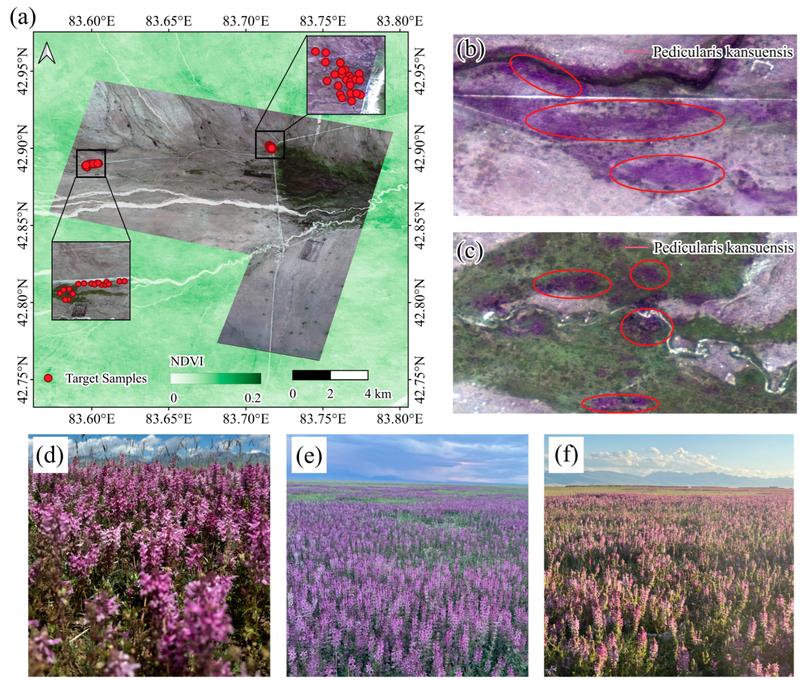
2.1. Study Area
2.2. Data
2.2.1. Satellite Imagery
2.2.2. Field Surveying Samples
3. Methods
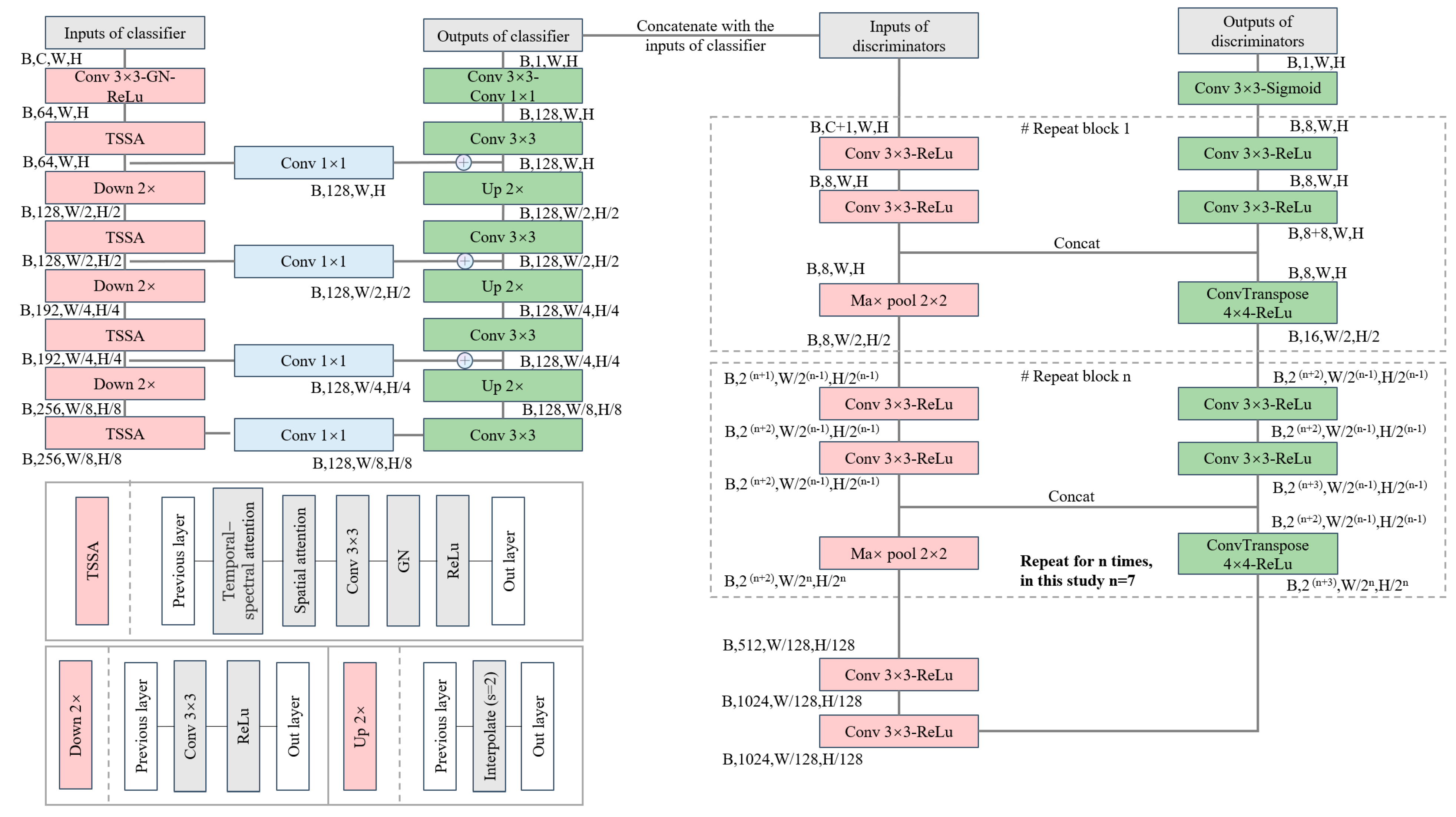
3.1. Architecture
3.2. The Class Prior-Free Classifier and Dual-Branch Discriminators
3.2.1. Class Prior-Free Classifier
3.2.2. Dual-Branch Discriminators
3.3. Loss Function
4. Experiments and Analysis
4.1. Experimental Preparation
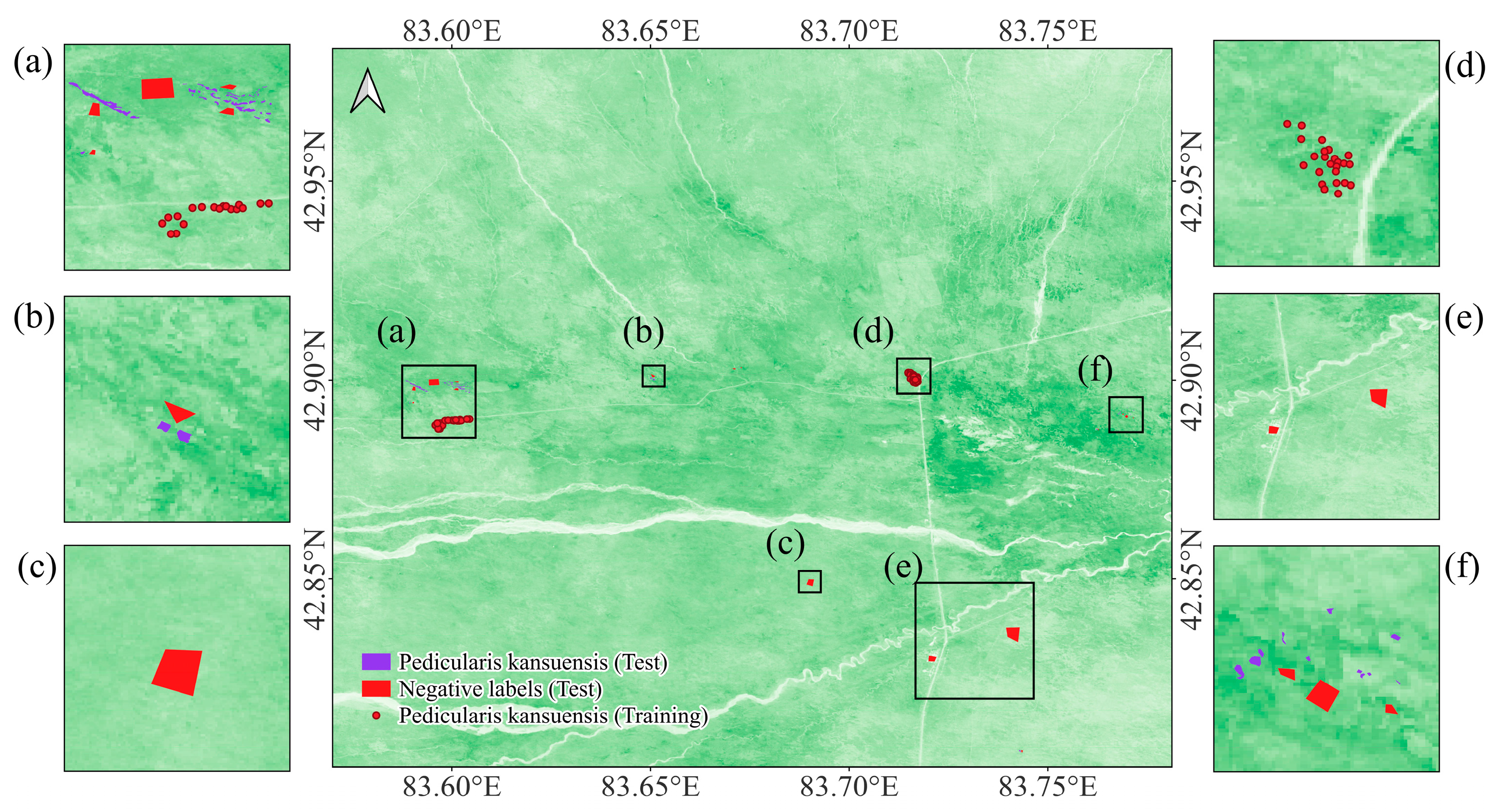
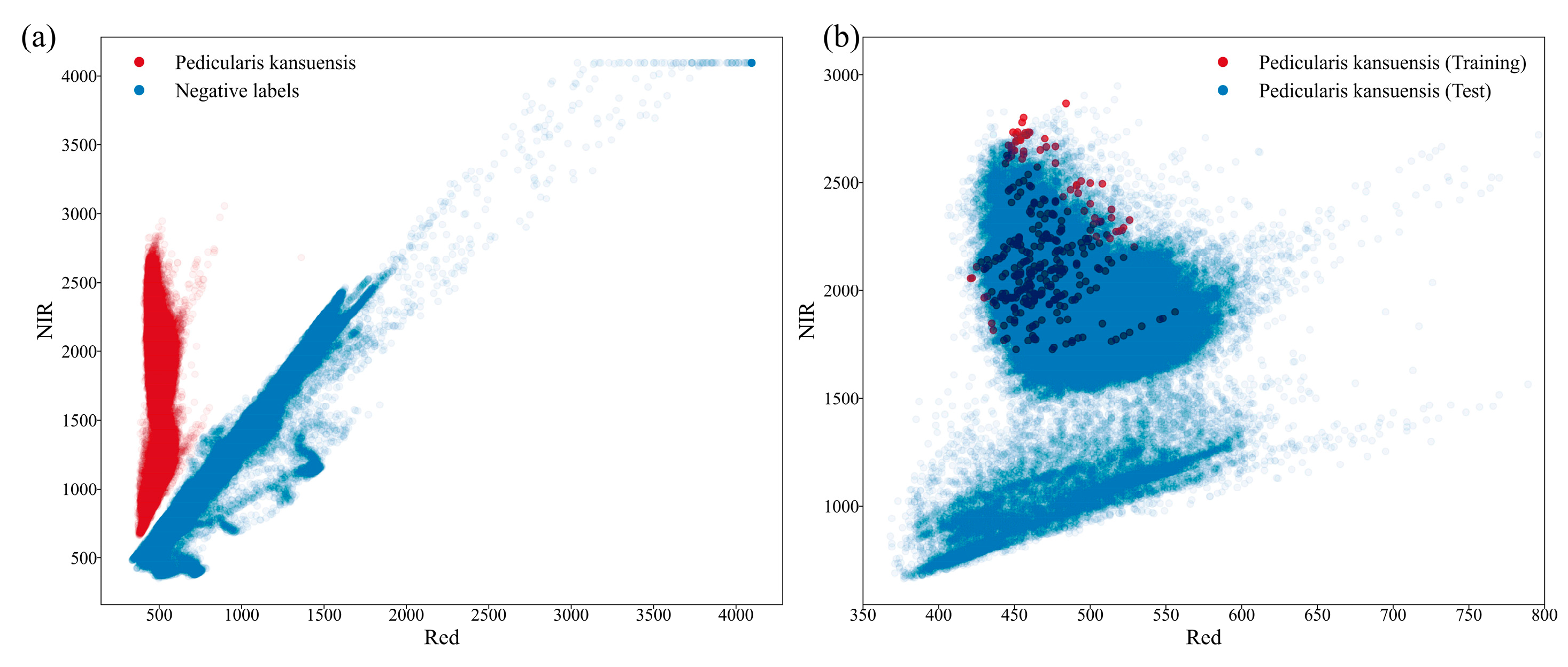
4.1.1. Datasets Preparation
4.1.2. Experimental Setting
4.1.3. Evaluation Methods and Metrics
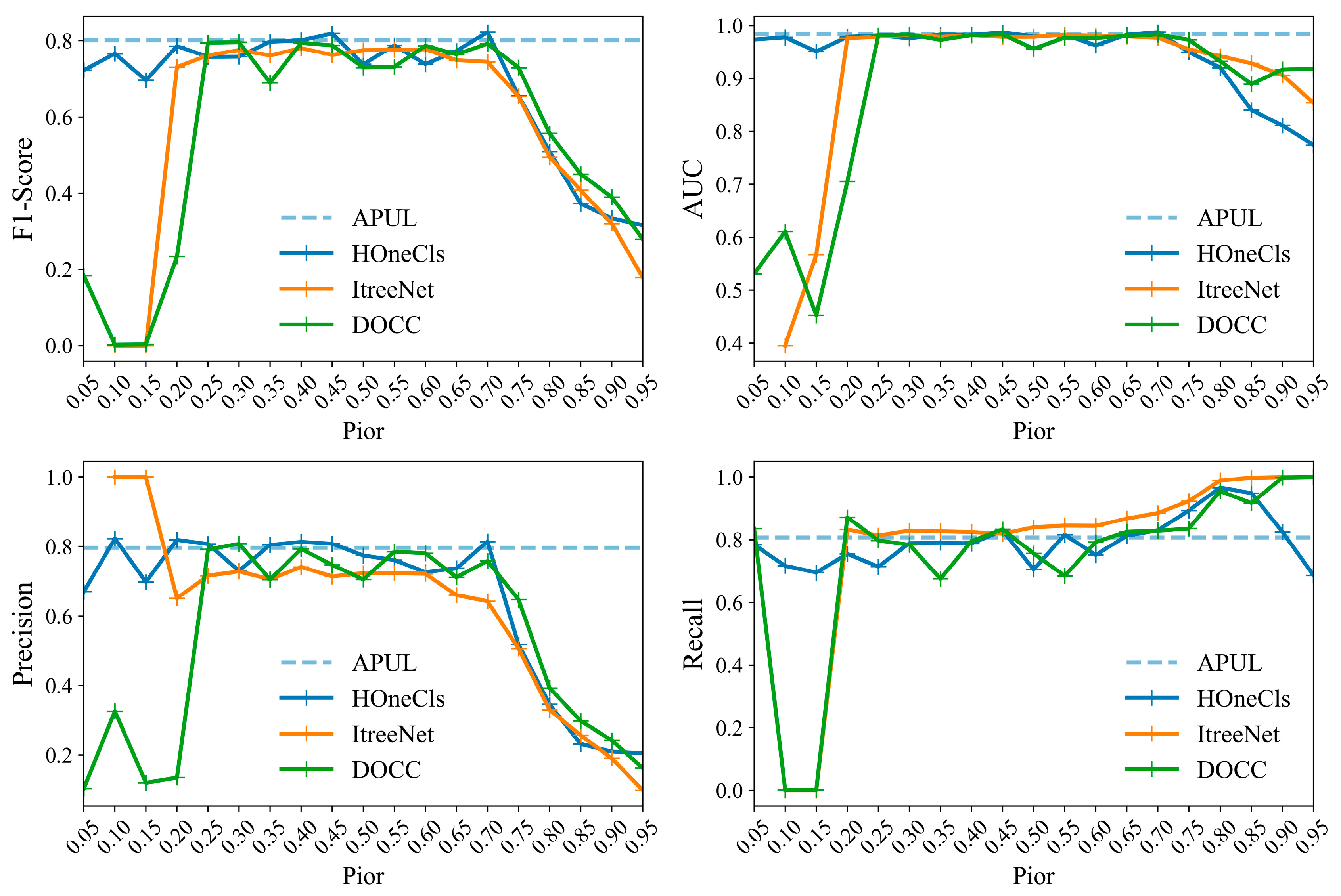
4.2. Experimental Results and Analysis
4.3. Ablation Experiment
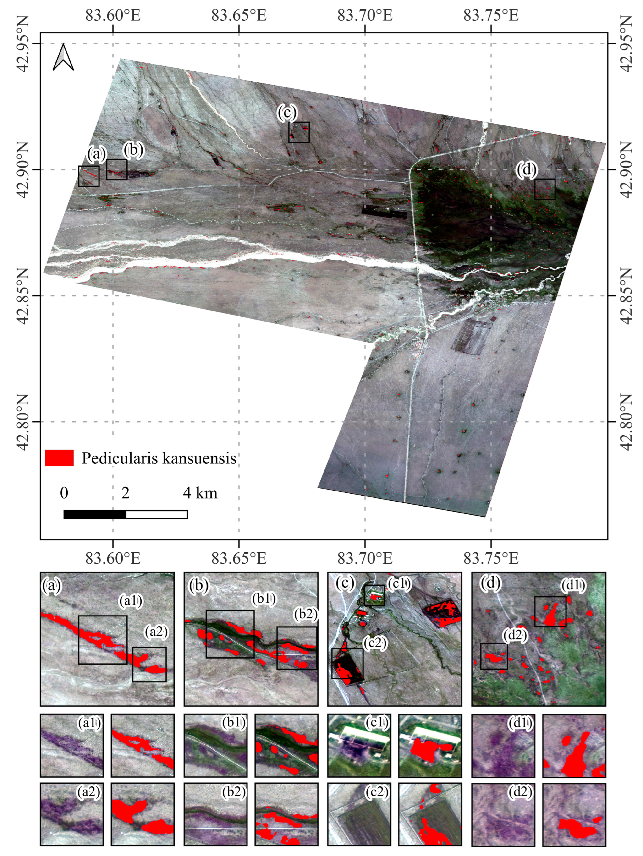
4.4. Pedicularis kansuensis in the Bayinbuluke Grassland
5. Discussion
6. Conclusions
- The APUL framework demonstrates superior performance in the task of extracting invasive Pedicularis kansuensis in the Bayinbuluke Grassland, Xinjiang. It achieves an F1-score of 0.8013 using only 42 positive samples, outperforming existing PUL methods.
- The dual-branch discriminators can enhance the performance of the classifier through a continuous adversarial process. Furthermore, the class prior-free classifier utilizing Taylor’s variational loss function can achieve a better performance comparable to other methods with the class prior probabilities.
- The proposed APUL framework identifies 178.27 hm2 of invasive Pedicularis kansuensis within the Bayinbuluke Grassland study area, accounting for 4.43% of the total vegetation area in the region. This proportion indicates that the invasion of Pedicularis kansuensis has significantly impacted the survival space of local pasture grasses.
Supplementary Materials
Author Contributions
Funding
Data Availability Statement
Acknowledgments
Conflicts of Interest
References
- Bonan, G.B. Forests and climate change: Forcings, feedbacks, and the climate benefits of forests. Science 2008, 320, 1444–1449. [Google Scholar] [CrossRef] [PubMed]
- Pan, Y.; Birdsey, R.A.; Fang, J.; Houghton, R.; Kauppi, P.E.; Kurz, W.A.; Phillips, O.L.; Shvidenko, A.; Lewis, S.L.; Canadell, J.G. A large and persistent carbon sink in the world’s forests. Science 2011, 333, 988–993. [Google Scholar] [CrossRef]
- Cardinale, B.J.; Duffy, J.E.; Gonzalez, A.; Hooper, D.U.; Perrings, C.; Venail, P.; Narwani, A.; Mace, G.M.; Tilman, D.; Wardle, D.A. Biodiversity loss and its impact on humanity. Nature 2012, 486, 59–67. [Google Scholar] [CrossRef] [PubMed]
- Pimentel, D.; Harvey, C.; Resosudarmo, P.; Sinclair, K.; Kurz, D.; McNair, M.; Crist, S.; Shpritz, L.; Fitton, L.; Saffouri, R. Environmental and economic costs of soil erosion and conservation benefits. Science 1995, 267, 1117–1123. [Google Scholar] [CrossRef] [PubMed]
- Vilà, M.; Espinar, J.L.; Hejda, M.; Hulme, P.E.; Jarošík, V.; Maron, J.L.; Pergl, J.; Schaffner, U.; Sun, Y.; Pyšek, P. Ecological impacts of invasive alien plants: A meta-analysis of their effects on species, communities and ecosystems. Ecol. Lett. 2011, 14, 702–708. [Google Scholar] [CrossRef]
- Ehrenfeld, J.G. Ecosystem consequences of biological invasions. Annu. Rev. Ecol. Evol. Syst. 2010, 41, 59–80. [Google Scholar] [CrossRef]
- Pimentel, D.; Zuniga, R.; Morrison, D. Update on the environmental and economic costs associated with alien-invasive species in the United States. Ecol. Econ. 2005, 52, 273–288. [Google Scholar] [CrossRef]
- Meyerson, L.A.; Mooney, H.A. Invasive alien species in an era of globalization. Front. Ecol. Environ. 2007, 5, 199–208. [Google Scholar] [CrossRef]
- Seebens, H.; Bacher, S.; Blackburn, T.M.; Capinha, C.; Dawson, W.; Dullinger, S.; Genovesi, P.; Hulme, P.E.; Van Kleunen, M.; Kühn, I. Projecting the continental accumulation of alien species through to 2050. Glob. Change Biol. 2021, 27, 970–982. [Google Scholar] [CrossRef]
- Hameed, A.; Zafar, M.; Ahmad, M.; Sultana, S.; Bahadur, S.; Anjum, F.; Shuaib, M.; Taj, S.; Irm, M.; Altaf, M.A. Chemo-taxonomic and biological potential of highly therapeutic plant Pedicularis groenlandica Retz. using multiple microscopic techniques. Microsc. Res. Tech. 2021, 84, 2890–2905. [Google Scholar] [CrossRef]
- Wang, X.; Zhang, Z.; Yu, Z.; Shen, G.; Cheng, H.; Tao, S. Composition and diversity of soil microbial communities in the alpine wetland and alpine forest ecosystems on the Tibetan Plateau. Sci. Total Environ. 2020, 747, 141358. [Google Scholar] [CrossRef]
- Callaway, R.M.; Aschehoug, E.T. Invasive plants versus their new and old neighbors: A mechanism for exotic invasion. Science 2000, 290, 521–523. [Google Scholar] [CrossRef] [PubMed]
- Williamson, M. Biological Invasions; Springer Science & Business Media: Berlin/Heidelberg, Germany, 1996. [Google Scholar]
- Diagne, C.; Leroy, B.; Vaissière, A.-C.; Gozlan, R.E.; Roiz, D.; Jarić, I.; Salles, J.-M.; Bradshaw, C.J.; Courchamp, F. High and rising economic costs of biological invasions worldwide. Nature 2021, 592, 571–576. [Google Scholar] [CrossRef]
- Rango, A.; Laliberte, A.; Herrick, J.E.; Winters, C.; Havstad, K.; Steele, C.; Browning, D. Unmanned aerial vehicle-based remote sensing for rangeland assessment, monitoring, and management. J. Appl. Remote Sens. 2009, 3, 033542. [Google Scholar]
- Getzin, S.; Wiegand, K.; Schöning, I. Assessing biodiversity in forests using very high-resolution images and unmanned aerial vehicles. Methods Ecol. Evol. 2012, 3, 397–404. [Google Scholar] [CrossRef]
- Xie, Y.; Sha, Z.; Yu, M. Remote sensing imagery in vegetation mapping: A review. J. Plant Ecol. 2008, 1, 9–23. [Google Scholar] [CrossRef]
- Adam, E.; Mutanga, O.; Rugege, D. Multispectral and hyperspectral remote sensing for identification and mapping of wetland vegetation: A review. Wetl. Ecol. Manag. 2010, 18, 281–296. [Google Scholar] [CrossRef]
- Gould, W. Remote sensing of vegetation, plant species richness, and regional biodiversity hotspots. Ecol. Appl. 2000, 10, 1861–1870. [Google Scholar] [CrossRef]
- Kerr, J.T.; Ostrovsky, M. From space to species: Ecological applications for remote sensing. Trends Ecol. Evol. 2003, 18, 299–305. [Google Scholar] [CrossRef]
- Bradley, B.A. Remote detection of invasive plants: A review of spectral, textural and phenological approaches. Biol. Invasions 2014, 16, 1411–1425. [Google Scholar] [CrossRef]
- Hudson, H.L.; Sesnie, S.E.; Hiebert, R.D.; Dickson, B.G.; Thomas, L.P. Crossjurisdictional monitoring for nonnative plant invasions using NDVI change detection indices in walnut canyon national monument, Arizona, USA. In The Colorado Plateau VI: Science and Management at the Landscape Scale; The University of Aeizona Press: Tucson, AZ, USA, 2015; pp. 23–40. [Google Scholar]
- Blumenthal, D.M.; Norton, A.P.; Cox, S.E.; Hardy, E.M.; Liston, G.E.; Kennaway, L.; Booth, D.T.; Derner, J.D. Linaria dalmatica invades south-facing slopes and less grazed areas in grazing-tolerant mixed-grass prairie. Biol. Invasions 2012, 14, 395–404. [Google Scholar] [CrossRef]
- Peerbhay, K.; Mutanga, O.; Lottering, R.; Ismail, R. Mapping Solanum mauritianum plant invasions using WorldView-2 imagery and unsupervised random forests. Remote Sens. Environ. 2016, 182, 39–48. [Google Scholar] [CrossRef]
- Cho, M.A.; Mathieu, R.; Asner, G.P.; Naidoo, L.; Van Aardt, J.; Ramoelo, A.; Debba, P.; Wessels, K.; Main, R.; Smit, I.P. Mapping tree species composition in South African savannas using an integrated airborne spectral and LiDAR system. Remote Sens. Environ. 2012, 125, 214–226. [Google Scholar] [CrossRef]
- Wäldchen, J.; Mäder, P. Machine learning for image based species identification. Methods Ecol. Evol. 2018, 9, 2216–2225. [Google Scholar] [CrossRef]
- Zhang, H.; He, G.; Peng, J.; Kuang, Z.; Fan, J. Deep learning of path-based tree classifiers for large-scale plant species identification. In Proceedings of the 2018 IEEE Conference on Multimedia Information Processing and Retrieval (MIPR), Miami, FL, USA, 10–12 April 2018; pp. 25–30. [Google Scholar]
- Pu, R. Mapping tree species using advanced remote sensing technologies: A state-of-the-art review and perspective. J. Remote Sens. 2021, 2021, 9812624. [Google Scholar] [CrossRef]
- Lake, T.A.; Briscoe Runquist, R.D.; Moeller, D.A. Deep learning detects invasive plant species across complex landscapes using Worldview-2 and Planetscope satellite imagery. Remote Sens. Ecol. Conserv. 2022, 8, 875–889. [Google Scholar] [CrossRef]
- James, K.; Bradshaw, K. Detecting plant species in the field with deep learning and drone technology. Methods Ecol. Evol. 2020, 11, 1509–1519. [Google Scholar] [CrossRef]
- Wang, Q.; Cheng, M.; Xiao, X.; Yuan, H.; Zhu, J.; Fan, C.; Zhang, J. An image segmentation method based on deep learning for damage assessment of the invasive weed Solanum rostratum Dunal. Comput. Electron. Agric. 2021, 188, 106320. [Google Scholar] [CrossRef]
- Thompson, N.C.; Greenewald, K.; Lee, K.; Manso, G.F. The computational limits of deep learning. arXiv 2020, arXiv:2007.05558. [Google Scholar]
- Zhu, X.X.; Tuia, D.; Mou, L.; Xia, G.-S.; Zhang, L.; Xu, F.; Fraundorfer, F. Deep learning in remote sensing: A comprehensive review and list of resources. IEEE Geosci. Remote Sens. Mag. 2017, 5, 8–36. [Google Scholar] [CrossRef]
- Sun, X.; Wang, B.; Wang, Z.; Li, H.; Li, H.; Fu, K. Research progress on few-shot learning for remote sensing image interpretation. IEEE J. Sel. Top. Appl. Earth Obs. Remote Sens. 2021, 14, 2387–2402. [Google Scholar] [CrossRef]
- Kiryo, R.; Niu, G.; Du Plessis, M.C.; Sugiyama, M. Positive-unlabeled learning with non-negative risk estimator. In Proceedings of the Advances in Neural Information Processing Systems (NIPS 2017), Long Beach, CA, USA, 4–9 December 2017; Volume 30. [Google Scholar]
- Jaskie, K.; Spanias, A. Positive Unlabeled Learning; Morgan & Claypool Publishers: San Rafael, CA, USA, 2022. [Google Scholar]
- Li, W.; Guo, Q.; Elkan, C. A positive and unlabeled learning algorithm for one-class classification of remote-sensing data. IEEE Trans. Geosci. Remote Sens. 2010, 49, 717–725. [Google Scholar] [CrossRef]
- Hu, W.; Le, R.; Liu, B.; Ji, F.; Ma, J.; Zhao, D.; Yan, R. Predictive adversarial learning from positive and unlabeled data. In Proceedings of the AAAI conference on artificial intelligence, Virtual Event, 2–9 February 2021; pp. 7806–7814. [Google Scholar]
- Bao, A.; Cao, X.; Chen, X.; Xia, Y. Study on models for monitoring of above ground biomass about Bayinbuluke grassland assisted by remote sensing. In Proceedings of the Remote Sensing and Modeling of Ecosystems for Sustainability V, San Diego, CA, USA, 10–14 August 2008; pp. 155–163. [Google Scholar]
- Liu, Q.; Yang, Z.; Han, F.; Shi, H.; Wang, Z.; Chen, X. Ecological environment assessment in world natural heritage site based on remote-sensing data. A case study from the Bayinbuluke. Sustainability 2019, 11, 6385. [Google Scholar] [CrossRef]
- Chen, X.; Yang, Z.; Wang, T.; Han, F. Landscape Ecological Risk and Ecological Security Pattern Construction in World Natural Heritage Sites: A Case Study of Bayinbuluke, Xinjiang, China. ISPRS Int. J. Geo-Inf. 2022, 11, 328. [Google Scholar] [CrossRef]
- Yanyan, L.; Yukun, H.; Jianmei, Y.; Kaihui, L.; Guogang, G.; Xin, W. Study on harmfulness of Pedicularis myriophylla and its control measures. Arid Zone Res 2008, 25, 778–782. [Google Scholar]
- Sui, X.; Li, A.; Guan, K. Impacts of climatic changes as well as seed germination characteristics on the population expansion of Pedicularis verticillata. Ecol. Environ. Sci 2013, 22, 1099–1104. [Google Scholar]
- Wang, W.; Tang, J.; Zhang, N.; Wang, Y.; Xu, X.; Zhang, A. Spatiotemporal Pattern of Invasive Pedicularis in the Bayinbuluke Land, China, during 2019–2021: An Analysis Based on PlanetScope and Sentinel-2 Data. Remote Sens. 2023, 15, 4383. [Google Scholar] [CrossRef]
- He, Z.; He, D.; Mei, X.; Hu, S. Wetland classification based on a new efficient generative adversarial network and Jilin-1 satellite image. Remote Sens. 2019, 11, 2455. [Google Scholar] [CrossRef]
- Gorelick, N.; Hancher, M.; Dixon, M.; Ilyushchenko, S.; Thau, D.; Moore, R. Google Earth Engine: Planetary-scale geospatial analysis for everyone. Remote Sens. Environ. 2017, 202, 18–27. [Google Scholar] [CrossRef]
- Pettorelli, N.; Vik, J.O.; Mysterud, A.; Gaillard, J.-M.; Tucker, C.J.; Stenseth, N.C. Using the satellite-derived NDVI to assess ecological responses to environmental change. Trends Ecol. Evol. 2005, 20, 503–510. [Google Scholar] [CrossRef]
- Gao, B.-C. NDWI—A normalized difference water index for remote sensing of vegetation liquid water from space. Remote Sens. Environ. 1996, 58, 257–266. [Google Scholar] [CrossRef]
- Zheng, Z.; Zhong, Y.; Ma, A.; Zhang, L. FPGA: Fast patch-free global learning framework for fully end-to-end hyperspectral image classification. IEEE Trans. Geosci. Remote Sens. 2020, 58, 5612–5626. [Google Scholar] [CrossRef]
- Woo, S.; Park, J.; Lee, J.-Y.; Kweon, I.S. Cbam: Convolutional block attention module. In Proceedings of the European Conference on Computer Vision (ECCV), Munich, Germany, 8–14 September 2018; pp. 3–19. [Google Scholar]
- Ronneberger, O.; Fischer, P.; Brox, T. U-net: Convolutional networks for biomedical image segmentation. In Proceedings of the Medical Image Computing and Computer-Assisted Intervention–MICCAI 2015: 18th International Conference, Munich, Germany, 5–9 October 2015; pp. 234–241. [Google Scholar]
- Chen, H.; Li, Z.; Wu, J.; Xiong, W.; Du, C. SemiRoadExNet: A semi-supervised network for road extraction from remote sensing imagery via adversarial learning. ISPRS J. Photogramm. Remote Sens. 2023, 198, 169–183. [Google Scholar] [CrossRef]
- Bekker, J.; Davis, J. Learning from positive and unlabeled data: A survey. Mach. Learn. 2020, 109, 719–760. [Google Scholar] [CrossRef]
- Li, W.; Guo, Q.; Elkan, C. One-class remote sensing classification from positive and unlabeled background data. IEEE J. Sel. Top. Appl. Earth Obs. Remote Sens. 2020, 14, 730–746. [Google Scholar] [CrossRef]
- Zhao, H.; Zhong, Y.; Wang, X.; Hu, X.; Luo, C.; Boitt, M.; Piiroinen, R.; Zhang, L.; Heiskanen, J.; Pellikka, P. Mapping the distribution of invasive tree species using deep one-class classification in the tropical montane landscape of Kenya. ISPRS J. Photogramm. Remote Sens. 2022, 187, 328–344. [Google Scholar] [CrossRef]
- Chen, H.; Liu, F.; Wang, Y.; Zhao, L.; Wu, H. A variational approach for learning from positive and unlabeled data. Adv. Neural Inf. Process. Syst. 2020, 33, 14844–14854. [Google Scholar]
- Zhao, H.; Wang, X.; Li, J.; Zhong, Y. Class prior-free positive-unlabeled learning with Taylor variational loss for hyperspectral remote sensing imagery. In Proceedings of the IEEE/CVF International Conference on Computer Vision, Paris, France, 1–6 October 2023; pp. 16827–16836. [Google Scholar]
- Pan, Z.; Yu, W.; Wang, B.; Xie, H.; Sheng, V.S.; Lei, J.; Kwong, S. Loss functions of generative adversarial networks (GANs): Opportunities and challenges. IEEE Trans. Emerg. Top. Comput. Intell. 2020, 4, 500–522. [Google Scholar] [CrossRef]
- Schölkopf, B.; Williamson, R.C.; Smola, A.; Shawe-Taylor, J.; Platt, J. Support vector method for novelty detection. In Proceedings of the Advances in Neural Information Processing Systems (NIPS 1999), Denver, CO, USA, 29 November–4 December 1999; Volume 12. [Google Scholar]
- Liu, B.; Dai, Y.; Li, X.; Lee, W.S.; Yu, P.S. Building text classifiers using positive and unlabeled examples. In Proceedings of the Third IEEE international conference on data mining, Melbourne, FL, USA, 22 November 2003; pp. 179–186. [Google Scholar]
- Lei, L.; Wang, X.; Zhong, Y.; Zhao, H.; Hu, X.; Luo, C. DOCC: Deep one-class crop classification via positive and unlabeled learning for multi-modal satellite imagery. Int. J. Appl. Earth Obs. Geoinf. 2021, 105, 102598. [Google Scholar] [CrossRef]
- Zhao, H.; Zhong, Y.; Wang, X.; Shu, H. One-class risk estimation for one-class hyperspectral image classification. IEEE Trans. Geosci. Remote Sens. 2023, 61, 1–17. [Google Scholar] [CrossRef]
- Schölkopf, B.; Platt, J.C.; Shawe-Taylor, J.; Smola, A.J.; Williamson, R.C. Estimating the support of a high-dimensional distribution. Neural Comput. 2001, 13, 1443–1471. [Google Scholar] [CrossRef] [PubMed]
- Cabezas, M.; Kentsch, S.; Tomhave, L.; Gross, J.; Caceres, M.L.L.; Diez, Y. Detection of invasive species in wetlands: Practical DL with heavily imbalanced data. Remote Sens. 2020, 12, 3431. [Google Scholar] [CrossRef]
- Royimani, L.; Mutanga, O.; Odindi, J.; Dube, T.; Matongera, T.N. Advancements in satellite remote sensing for mapping and monitoring of alien invasive plant species (AIPs). Phys. Chem. Earth Parts A/B/C 2019, 112, 237–245. [Google Scholar] [CrossRef]
- Weisberg, P.J.; Dilts, T.E.; Greenberg, J.A.; Johnson, K.N.; Pai, H.; Sladek, C.; Kratt, C.; Tyler, S.W.; Ready, A. Phenology-based classification of invasive annual grasses to the species level. Remote Sens. Environ. 2021, 263, 112568. [Google Scholar] [CrossRef]
- Madonsela, S.; Cho, M.A.; Mathieu, R.; Mutanga, O.; Ramoelo, A.; Kaszta, Ż.; Van De Kerchove, R.; Wolff, E. Multi-phenology WorldView-2 imagery improves remote sensing of savannah tree species. Int. J. Appl. Earth Obs. Geoinf. 2017, 58, 65–73. [Google Scholar] [CrossRef]
- Kattenborn, T.; Leitloff, J.; Schiefer, F.; Hinz, S. Review on Convolutional Neural Networks (CNN) in vegetation remote sensing. ISPRS J. Photogramm. Remote Sens. 2021, 173, 24–49. [Google Scholar] [CrossRef]


| Satellites | Jilin-1 | Sentinel-2 | ||||
|---|---|---|---|---|---|---|
| Band | Spatial resolution | Wavelength (nm) | Band | Spatial resolution | Wavelength (nm) | |
| Spectral bands | B1 | 0.75 m | 450–700 | B1 | 60 m | 433–453 |
| B2 | 3 m | 430–520 | B2 | 10 m | 458–523 | |
| B3 | 3 m | 520–610 | B3 | 10 m | 543–578 | |
| B4 | 3 m | 610–690 | B4 | 10 m | 650–680 | |
| B5 | 3 m | 770–895 | B5 | 20 m | 698–713 | |
| B6 | 20 m | 733–748 | ||||
| B7 | 20 m | 773–793 | ||||
| B8 | 10 m | 785–900 | ||||
| B8A | 20 m | 855–875 | ||||
| B9 | 60 m | 935–955 | ||||
| B10 | 60 m | 1360–1390 | ||||
| B11 | 20 m | 1565–1655 | ||||
| B12 | 20 m | 2100–2280 | ||||
| Band number | 4 spectral bands and 2 index bands (Without B1) | 13 spectral bands and 2 index bands | ||||
| Revisiting Period (Days) | 3.3 | 5 | ||||
| Date | 10 August 2023 | July, August, September 2023 | ||||
| Classifier (FCN) | Discriminators (UNet) | |
|---|---|---|
| Encoder |
Conv 3
×
3, stride 1, 64 TSSA#1: Conv 3 × 3, stride 1, 64 Down 2 × #1: Conv 3 × 3, stride 2128 TSSA#2: Conv 3 × 3, stride 1, 128 Down 2 × #2: Conv 3 × 3, stride 2192 TSSA#3: Conv 3 × 3, stride 1, 192 Down 2 × #3: Conv 3 × 3, stride 2256 TSSA#4: Conv 3 × 3, stride 1, 256 |
Conv 3
×
3, stride 1, 8 Conv 3 × 3, stride 1, 8 Conv 3 × 3, stride 1, 16 Conv 3 × 3, stride 1, 16 Conv 3 × 3, stride 1, 32 Conv 3 × 3, stride 1, 32 Conv 3 × 3, stride 1, 64 Conv 3 × 3, stride 1, 64 Conv 3 × 3, stride 1, 128 Conv 3 × 3, stride 1, 128 Conv 3 × 3, stride 1, 256 Conv 3 × 3, stride 1, 256 Conv 3 × 3, stride 1, 512 Conv 3 × 3, stride 1, 512 Conv 3 × 3, stride 1, 1024 Conv 3 × 3, stride 1, 1024 |
| Lateral | Conv1 × 1, stride 1, 128 | None |
| Decoder |
Conv3
×
3, stride 1, 128 Conv3 × 3, stride 1, 128 Conv3 × 3, stride 1, 128 Conv3 × 3, stride 1, 128 Conv3 × 3, stride 1, 128 Conv 3 × 3, stride 1, 64 Conv 1 × 1, stride 1, 1 |
ConvTranspose 4
×
4, stride 2512 Conv 3 × 3, stride 1, 512 Conv 3 × 3, stride 1, 512 ConvTranspose 4 × 4, stride 2256 Conv 3 × 3, stride 1, 256 Conv 3 × 3, stride 1, 256 ConvTranspose 4 × 4, stride 2127 Conv 3 × 3, stride 1, 128 Conv 3 × 3, stride 1, 128 ConvTranspose 4 × 4, stride 2, 64 Conv 3 × 3, stride 1, 64 Conv 3 × 3, stride 1, 64 ConvTranspose 4 × 4, stride 2, 32 Conv 3 × 3, stride 1, 32 Conv 3 × 3, stride 1, 32 ConvTranspose 4 × 4, stride 2, 16 Conv 3 × 3, stride 1, 16 Conv 3 × 3, stride 1, 16 ConvTranspose 4 × 4, stride 2, 8 Conv 3 × 3, stride 1, 8 Conv 3 × 3, stride 1, 8 Conv 3 × 3, stride 1, 1 |
| Characteristics | Size (Pixels) | Labeling Methods | |
|---|---|---|---|
| Training set | 51 bands | Positive: 304 Unlabeled: 1,048,272 | Field sampling |
| Test set | 51 bands | Positive: 55,525 Negative: 125,195 | Visual interpretation |
| Type | Model | AUC | Precision | Recall | F1-Score |
|---|---|---|---|---|---|
| One-class machine learning | OCSVM | 0.6291 | 0.1727 | 0.5275 | 0.2601 |
| BSVM | 0.6438 | 0.3677 | 0.6050 | 0.4431 | |
| Deep PUL with class prior probabilities | ItreeNet | 0.9805 | 0.7370 | 0.8307 | 0.7802 |
| DOCC | 0.9775 | 0.7529 | 0.7935 | 0.7707 | |
| HOneCls | 0.9818 | 0.7920 | 0.7842 | 0.7868 | |
| Class prior-free Deep PUL | T-HOneCls | 0.9679 | 0.6782 | 0.8315 | 0.7464 |
| APUL | 0.9842 | 0.7963 | 0.8072 | 0.8013 |
| Backbone | Structure | Loss | Dataset | Precision | Recall | F1- Score |
|---|---|---|---|---|---|---|
| FCN | None | BCE | Jilin-1 | 0.4049 | 0.9684 | 0.5639 |
| Jilin-1 & Sentinel2 | 0.4367 | 0.987 | 0.6055 | |||
| Taylor | Jilin-1 | 0.7555 | 0.7426 | 0.7485 | ||
| Jilin-1 & Sentinel2 | 0.7402 | 0.7733 | 0.7534 | |||
| Adversarial | BCE | Jilin-1 | 0.3395 | 0.9991 | 0.5059 | |
| Jilin-1 & Sentinel2 | 0.4032 | 0.9883 | 0.5703 | |||
| Taylor | Jilin-1 | 0.7757 | 0.7909 | 0.7817 | ||
| Jilin-1 & Sentinel2 | 0.7963 | 0.8072 | 0.8013 |
Disclaimer/Publisher’s Note: The statements, opinions and data contained in all publications are solely those of the individual author(s) and contributor(s) and not of MDPI and/or the editor(s). MDPI and/or the editor(s) disclaim responsibility for any injury to people or property resulting from any ideas, methods, instructions or products referred to in the content. |
© 2025 by the authors. Licensee MDPI, Basel, Switzerland. This article is an open access article distributed under the terms and conditions of the Creative Commons Attribution (CC BY) license (https://creativecommons.org/licenses/by/4.0/).
Share and Cite
Zhu, E.; Samat, A.; Li, E.; Xu, R.; Li, W.; Li, W. Adversarial Positive-Unlabeled Learning-Based Invasive Plant Detection in Alpine Wetland Using Jilin-1 and Sentinel-2 Imageries. Remote Sens. 2025, 17, 1041. https://doi.org/10.3390/rs17061041
Zhu E, Samat A, Li E, Xu R, Li W, Li W. Adversarial Positive-Unlabeled Learning-Based Invasive Plant Detection in Alpine Wetland Using Jilin-1 and Sentinel-2 Imageries. Remote Sensing. 2025; 17(6):1041. https://doi.org/10.3390/rs17061041
Chicago/Turabian StyleZhu, Enzhao, Alim Samat, Erzhu Li, Ren Xu, Wei Li, and Wenbo Li. 2025. "Adversarial Positive-Unlabeled Learning-Based Invasive Plant Detection in Alpine Wetland Using Jilin-1 and Sentinel-2 Imageries" Remote Sensing 17, no. 6: 1041. https://doi.org/10.3390/rs17061041
APA StyleZhu, E., Samat, A., Li, E., Xu, R., Li, W., & Li, W. (2025). Adversarial Positive-Unlabeled Learning-Based Invasive Plant Detection in Alpine Wetland Using Jilin-1 and Sentinel-2 Imageries. Remote Sensing, 17(6), 1041. https://doi.org/10.3390/rs17061041