Abstract
Recently, hyperspectral image (HSI) mixed denoising methods based on nonlocal subspace representation (NSR) have achieved significant success. However, most of these methods focus on optimizing the denoiser for representation coefficient images (RCIs) without considering how to construct RCIs that better inherit the spatial structure of the clean HSI, thereby affecting subsequent denoising performance. Although existing works have constructed RCIs from the perspective of sparse principal component analysis (SPCA), the refinement of RCIs in mixed noise conditions still leaves much to be desired. To address the aforementioned challenges, in this paper, we reconstructed robust RCIs based on SPCA in mixed noise circumstances to better preserve the spatial structure of the clean HSI. Furthermore, we propose to utilize the robust RCIs as prior information and perform iterative denoising in the denoiser that incorporates low-rank approximation. Extensive experiments conducted on both simulated and real HSI datasets demonstrate that the proposed robust RCIs guidance and low-rank approximation method, denoted as RRGNLA, exhibits competitive performance in terms of mixed denoising accuracy and computational efficiency. For instance, on the Washington DC Mall (WDC) dataset in Case 3, the denoising quantitative metrics of the mean peak signal-to-noise ratio (MPSNR), mean structural similarity index (MSSIM), and spectral angle mean (SAM) are 36.06 dB, 0.963, and 3.449, respectively, with a running time of 35.24 s. On the Pavia University (PaU) dataset in Case 4, the denoising quantitative metrics of MPSNR, MSSIM, and SAM are 34.34 dB, 0.924, and 5.505, respectively, with a running time of 32.79 s.
1. Introduction
Hyperspectral images (HSIs) represent a type of three-dimensional data, acquired by sensors across hundreds of contiguous narrow spectral bands within the visible to infrared light range [1,2]. Due to the rich spatial information and high spectral resolution inherent in HSIs, they have been widely applied in various fields such as environmental monitoring [3], mineral exploration [4], and military security [5]. However, during the actual acquisition and transmission processes, HSIs are inevitably influenced by various types of mixed noise, including Gaussian noise and impulse noise, as well as interference factors such as deadlines and stripes. This contamination leads to a deterioration in imaging quality, which subsequently hinders the performance of HSIs in subsequent tasks such as detection [6] and recognition [7,8]. In order to improve the performance of subsequent tasks, HSI denoising has become an essential preprocessing step.
Currently, extensive research has been conducted on this issue, and various methods have been proposed to restore HSI. In the early stages of research, each band of HSI is treated as an independent grayscale image to facilitate the direct application of traditional denoising methods [9,10,11,12]. Although these methods are straightforward and easily implementable, they only consider the spatial characteristics of HSI while neglecting the correlation between spectra bands. In subsequent research, various denoising methods that take into account the spatial–spectral structure of HSI have been proposed consecutively [13,14,15,16,17,18]. In these methods, due to the inherently low-rank structure of HSIs [1], approaches based on low-rank matrix/tensor decomposition model have demonstrated superior performance. Furthermore, researchers have incorporated various prior information into this model, such as nonlocal self-similarity, to further enhance denoising performance [19,20,21,22,23]. Nonlocal self-similarity is an inherent characteristic of HSIs. The essence of utilizing this property for denoising is to reconstruct the current image patch by matching similar patches through a search window. However, due to the large spectral dimension of HSI, the block matching stage is generally time-consuming, which may not meet the rapid processing requirements of real-world HSI denoising tasks.
To address the aforementioned issues, HSI denoising methods based on nonlocal subspace representation (NSR) have garnered significant attention. These methods map HSI to a low-dimensional subspace, thereby enhancing denoising efficiency while also ensuring denoising performance [24,25,26,27,28,29,30,31]. Specifically, for a noisy HIS , we perform a low-rank decomposition to obtain an orthogonal matrix and a three-dimensional tensor . The face slices along the third mode of are called representation coefficient images (RCIs). Each RCI inherits the spatial structure of the clean HSI, which is the main reason why NSR-based methods can guarantee denoising performance. However, most of the NRS-based denoising methods focus on how to design a more effective RCIs denoiser while neglecting the optimization of RCIs itself, which also indicates that the denoising performance of HSI has the potential to be further improved.
In order to optimize RCIs, it is necessary to analyze why RCIs can inherit the spatial structure of the clean HSI. Recently, study [32] reanalyzed the subspace representation process of HSI from the perspective of principal component analysis (PCA) and explained that each RCI is actually a combination of the bands of the clean HSI. However, PCA is affected by the noise-corrupted bands when estimating RCIs, which results in RCIs not being able to inherit the spatial structure of clean HSI well. To alleviate this problem, ref. [32] developed an elastic net model based on sparse principal component analysis (SPCA) to estimate RCIs and proposed a novel HSI denoising method. However, the method proposed in [32] does not demonstrate satisfactory performance in the task of HSI mixed denoising. This is because, on the one hand, the method constructs RCIs by only considering Gaussian noise conditions, without adequately accounting for the effects of other types of noise and interference. On the other hand, the method lacks an iterative strategy for removing mixed noise.
Inspired by the aforementioned discussion, in this paper, we first propose a novel elastic network model based on SPCA to reconstruct robust RCIs under mixed noise conditions. This novel construction method mitigates the impact of mixed noise, enabling the RCIs to better inherit the spatial structure of the clean HSI. Furthermore, to further enhance denoising performance, we utilize the obtained RCIs as prior information, along with the other prior information (low-rank approximation of nonlocal similar RCI patches, see the subsequent description for details) to perform iterative denoising in the NSR-based denoiser. Different from other methods that optimize RCIs denoiser, our method gives more consideration to the construction of RCIs. We denote this novel HSI mixed denoising method via robust RCIs and nonlocal low-rank approximation as RRGNLA.
In summary, this paper presents the following three contributions:
- To adapt to the noise condition in real HSIs, we introduce the norm into the elastic net model based on SPCA to constrain sparse noise including impulse noise, deadlines, and stripes, thereby enabling the construction of robust RCIs.
- A mixed denoising model based on NSR is established, which utilizes the robust RCIs as prior information and takes into account nonlocal low-rank approximation. Moreover, we adopt the alternating direction method of multipliers (ADMMs) to solve the proposed RRGNLA model.
- The experimental results indicate that the proposed RRGNLA method demonstrates competitive performance in both denoising effect and computational efficiency compared with other state-of-the-art methods. In the majority of experimental results, RRGNLA consistently achieves optimal denoising performance with high computational efficiency.
Notations: In this paper, lowercase x, uppercase X, bold uppercase X, and uppercase cursive denote scalar, vector, matrix, and tensor, respectively. For a p-order tensor , its unfolding is denoted as . The mode-j product of a tensor and a matrix is denoted as , which is equivalent to , where . The Frobenius norm and norm of X are defined as and , respectively, where is the inner product of X and itself, and denotes the element in the i-th row and j-th column of X.
The rest of this paper is organized as follows: Section 2 briefly introduces related work. In Section 3, we first discuss the elastic network model for estimating RCIs in mixed noise circumstances and provide the corresponding solution algorithm. Subsequently, we elaborate on the proposed RRGNLA model and its corresponding optimization algorithm. Section 4 presents and discusses the experimental results under both simulated and real HSI datasets. Finally, Section 5 concludes this paper.
2. Related Work
As mentioned above, in early studies, some classic visible light image denoising methods were applied to HSI denoising. For example, Rasti et al. [9] applied wavelet transform for sparse low-rank regression. Zhao et al. [10] first analyzed the low-rank characteristic of HSI, then utilized the theory of the KSVD algorithm to perform low-rank constraint and sparse approximation on HSI. Although these methods do not consider the spectral correlation of HSI, they have inspired subsequent research. Zhang et al. [13] sorted HSI by dictionary order to explore its low-rank property and removed noise using a low-rank matrix recovery method. Lu et al. [14] achieved noise-free estimation by grouping the spectral bands of HSI. Xue et al. [15] proposed a low-rank regularization method based on the spatial–spectral structure to characterize the spatial structure of HSI and perform denoising. To better preserve the spatial structure of HSI, Fan et al. [16] proposed a new tensor low-rank decomposition method to address the noise sensitivity problem during decomposition. Moreover, Huang et al. [17] also achieved notable HSI denoising performance by embedding group sparsity into low-rank tensor decomposition.
At the same time, total variation (TV) is widely utilized in tasks that involve removing heavy Gaussian noise. Fan et al. [19] proposed an HSI denoising method based on total variation (TV) regularization, which simultaneously considers the local spatial structure and the correlation among adjacent bands. Peng et al. [20] proposed an enhanced 3DTV regularization method to improve the denoising performance of HSI. In addition to TV, nonlocal self-similarity has also been widely utilized as prior information, demonstrating effective denoising performance. Sarkar et al. [21] employed the super-patch method to consider the redundancy between spatial and spectral aspects and then utilized the nuclear norm for the restoration of HSI. Xie et al. [22] designed a high-order sparsity metric and applied it to different HSI recovery tasks. Xue et al. [23] proposed a novel denoising method that leverages the spectral inter-correlation and nonlocal similarity inherent in HSI. Although utilizing nonlocal self-similarity has brought performance improvement to HSI denoising, it has, however, reduced the denoising efficiency.
Recently, NSR-based denoising methods have attracted increasing attention due to their superiority in denoising efficiency. The NSR-based denoising method usually converts the original denoising problem into the RCIs denoising problem first and then utilizes nonlocal self-similarity and different regularizations to optimize the design of the RCIs denoiser, thereby improving the computational efficiency while also ensuring the denoising performance. For instance, Zhuang et al. [24] directly utilized BM3D as the denoiser for RCIs, proposing a fast HSI denoising method. Furthermore, Zhuang et al. [25] proposed an RCIs denoiser based on successive singular value decomposition (SVD) to improve the performance. Lin et al. [26] introduced low tube rank into the RCIs denoiser to enhance HSI denoising performance.
To better adapt to the noise in real-world HSI, a lot of research progress has been made in NSR-based mixed denoising methods [33,34,35,36,37,38,39,40,41]. Sun et al. [33] applied superpixel HSI denoising, enhancing the overall denoising performance by imposing low-rank constraints on each superpixel block. Cao et al. [34] proposed a new denoising method based on nonlocal low-rank and sparse factorization. This method utilizes the norm to constrain the sparse noise component, further improving the denoising performance under mixed noise. Taking into account the common features and continuity among different bands, Zheng et al. [35] proposed a mixed denoising method based on dual-factor regularization. In addition, He et al. [36] proposed and applied high-dimensional (dimension greater than three) tensor SVD to better represent the structural correlation of HSI. This denoising method can compete with other state-of-the-art methods in terms of both denoising performance and computational efficiency.
These NSR-based mixed denoising methods demonstrate excellent performance by utilizing different regularization constraints within the denoiser. However, obtaining RCIs as a crucial step in NSR-based denoising methods has not been adequately considered for better construction. Although study [32] analyzed RCIs from the perspective of PCA and constructed new RCIs through an elastic network model based on SPCA, this elastic network model only considered the scenario of Gaussian noise, which deviates seriously from the real-world situation. In our proposed RRGNLA method, we reconstruct robust RCIs in mixed noise circumstances, which better preserve the spatial structures of the clean HSI. Unlike these NSR-based denoising methods that optimize RCIs denoisers, the proposed RRGNLA method simply incorporates a denoiser with WNNM low-rank regularization to ensure denoising efficiency. In the subsequent sections, ablation studies demonstrate the effectiveness of our constructed robust RCIs and iterative strategy in improving denoising performance. A more detailed discussion will be provided later.
3. Proposed Method
3.1. Problem Formulation
Here, let denote the three-dimensional noisy HSI data, where m and n denote the height and width of the HSI in the spatial domain, respectively, and b denotes the number of bands of the HSI in the spectra domain. , and denote three-dimensional data of the underlying clean HSI, Gaussian noise, and sparse noise (e.g., impulse noise, deadlines, and stripes), respectively. The degradation model of HSI under mixed noise can be expressed as:
According to the degradation Model (1), the denoising problem is transformed into how to better recover from . In general, the regularization model for removing mixed noise from HSI can be articulated as follows:
The first term is the data fidelity term, which can indirectly suppress Gaussian noise. The second term is a regularization term for the clean HSI. There are many different regularizers that optimize to obtain superior denoising performance. In this paper, due to the excellent performance of the weighted nuclear norm minimization (WNNM) low-rank regularizer [12] in various signal processing, we adopt it as the regularization term of , which will be explained in more detail in the following subsections. The third term is a regularization term for suppressing sparse noise. Parameters and , respectively, denote the weights of and , which are utilized to balance the importance of the two terms and can be dynamically adjusted. While the adjustment of parameters does influence the denoising performance of HSI, the selection of regularizers for different components plays a more crucial role.
3.2. Proposed Subspace Representation Model
Owing to the considerable correlation between spectral channels, HSIs inherently exhibit a low-rank structure [1]. Therefore, the clean HSI can be denoted by a subspace , where . Specifically, the latent clean HSI can be decomposed into:
where denotes model-3 tensor product, denotes the basis of subspace , E is orthogonal, i.e., with denoting the k-th order identity matrix. refers to the RCIs mentioned above. The E can be initialized using PCA (SVD) or other variants such as HySime [42]. The tensor can be obtained by projecting the noisy HSI onto the subspace, i.e., . Therefore, the NSR-based HSI denoising model can be written as:
In this paper, we assess the superiority of RCIs from the following two aspects. The first aspect is the ability to characterize the spatial structure of clean HSI, which directly impacts the performance of subsequent denoising processes. The second aspect is the capability to suppress mixed noise. If the construction of the RCIs involves a significant number of bands affected by mixed noise, the denoising performance will be notably compromised. Study [32] confirmed that SPCA demonstrates a strong capability in characterizing the spatial structure of clean HSI while also effectively suppressing Gaussian noise. Therefore, we employ a model based on SPCA to construct the RCIs. We introduce a norm constrained regularization term into the model to suppress sparse noise, proposing a novel elastic network model based on SPCA to construct RCIs in mixed noise circumstances:
where denotes the sparse coefficient matrix. The first term is the data fidelity term. The second and third terms are regularization terms, constrained by the norm and Frobenius norm, respectively. These terms are designed to enhance the sparsity of S and control its robustness. The fourth term is the regularization term for the sparse noise , which employs the norm constraint to regulate its sparsity. Parameters and are applied to S and , respectively. The larger the values of these parameters, the greater the sparsity of S and respectively. At the same time, regulates the robustness of . The three variables in Model (5) can be optimized separately through the ADMM algorithm, which is equivalent to solving three subproblems:
- 1.
- Update , the subproblem of optimizing is:where is the soft threshold operator [43].
- 2.
- Update E, the subproblem of optimizing E is:
The Frobenius norm in Equation (7) will be expanded and solved as follows:
Given the variables S and , the first two terms of Equation (8) are fixed values. Consequently, the problem of minimizing Equation (7) can be reformulated as maximizing the third term in Equation (8). The optimization problem can be rewritten as follows:
The orthogonality of E allows the following closed form [44,45]:
where denotes the singular value decomposition, and U and V denote the left and right singular vectors of the SVD decomposition, respectively.
- 3.
- Update S, the subproblem of optimizing S is:where the parameter is the scaling step size, and denotes the scaled soft threshold operator [45]:
By separately solving the three subproblems, we can obtain the robust RCIs that meet our requirements. The more detailed derivation and overall solution process are summarized in Appendix A and Algorithm 1, respectively. Based on the previous description, we can derive the expression for RCIs:
| Algorithm 1: Obtaining Robust RCIs via SPCA Operator |
| /* This algorithm obtains robust RCIs through iterative computation. This algorithm initializes variables using input noisy HSI . It continues until the relative error is below a specified threshold or the maximum number of iterations is reached. */ Input: the noisy HSI , the dimension of subspace k, and the parameters and 1: Initialization: , are estimated by SVD; Set t = 0, maximum iteration T, and 2: while not converged do 3: update via (6)//Iterative computation of the sparse noise. |
| 4: update via (10)//Iterative computation of the subspace basis. 5: update via (12)//Iterative computation of the sparse coefficient matrix. 6: check the convergence: or the error 7: update iteration: 8: end while 9: Compute via (13)//Obtain robust RCIs. Output: the robust RCIs and the orthogonal matrix |
3.3. Proposed RRGNLA Method
In previous studies, it has been demonstrated that various feature images in RCIs exhibit nonlocal self-similarity [34]. In order to achieve improved denoising performance, we utilize nonlocal self-similarity to construct similar 3D blocks from and then perform low-rank approximation on these similar 3D blocks.
Here, we introduce the construction process of self-similar 3D blocks. In order to facilitate subsequent descriptions, we articulate the construction process from a mathematical perspective. Set a search window of size , is the i-th 3D patch selected by the search window from , and is the spatial size of the 3D patch. First, we transform into a two-dimensional matrix of size . Next, using nonlocal self-similarity, we match the top s similar patches of (block matching), where s is the predetermined number of matches. Finally, the obtained similar patches are stacked into a similar block of size (stacking). We denote the above operation as , and the process of obtaining can be represented as . In order to facilitate comprehension, we also provide the flowchart of the process, as illustrated in Figure 1.
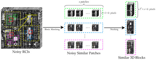
Figure 1.
Flowchart of constructing similar 3D blocks in this paper, where the yellow dashed square is the search window, the red square is the 3D patch, and the other color squares are similar patches.
Next, due to the superior performance of the WNNM low-rank regularizer [12], in this paper, we apply it for the low-rank approximation of :
where is the result of the low-rank approximation of the i-th 3D patch in . denotes the noise variance in , which can be derived from the noise variance in the noisy HSI . For the real HSI, can be estimated using Algorithm 1, presented in [42]. It is worth mentioning that, in this paper, since we performed whitening [25] on the noisy HSI before obtaining RCIs, the value of is 1. In the subsequent discussion, we will set directly.
Based on the above-mentioned analysis, we present the specific formulation of the proposed RRGLRA model as follows:
where in Model (15) is obtained through Algorithm 1, presented in this paper, serving as prior information to guide the subsequent denoising process. Simultaneously, as another prior information, aids the RRGLRA model in achieving enhanced denoising performance, which is manifested by the WNNM low-rank regularizer embedded in Model (15). Model (15) can be decoupled into the following two subproblems:
The solution to the subproblem in Equation (16) has already been explained in the previous section. Here, we focus on solving the subproblem in Equation (17). We also employ the model algorithm to optimize the three variables in the Equation (17) separately.
- 1.
- Update :where is the soft threshold operator, which is the same as in Equation (6).
- 2.
- Update :
This is a quadratic optimization problem, which can be solved by finding where the gradient of equals zero [34]. The closed-form of Equation (19) can be guaranteed as follows by the orthogonality of E:
From Equation (20), it is evident that the process of updating includes the inverse transformation of with as prior information.
- 3.
- Update E:
According to the analysis presented in [33], the solution form of Equation (21) is as follows:
where and are the left and right singular vectors obtained by performing SVD on .
In summary, the algorithmic procedure and flowchart of the proposed RRGNLA method can be referred to in Figure 2 and Algorithm 2, respectively.
| Algorithm 2: RRGNLA Method for HSI Mixed Denoising |
| /* This algorithm restores noisy HSI through iterative computation. It utilizes the robust RCIs from Algorithm 1 as prior information and embeds the WNNM low-rank regularizer into the iterative denoising process. */ Input: the noisy HSI , the dimension of subspace k, and the parameters and 1: Initialization: Set t = 0, maximum iteration T 2: Obtain and via Algorithm 1 //Utilize robust RCIs guidance for denoising. 3: Construct using l and s //Block matching and stacking similar patches. 4: Approximate Low-rank via (16) //Denoise using WNNM low-rank regularizer. 5: while not converged do 6: update via (18) //Iterative computation of the sparse noise. |
| 7: update via (20) //Iterative computation of the Robust RCIs. 8: update via (22) //Iterative computation of the orthogonal matrix. 9: check the convergence: 10: update iteration: 11: end while 12: Compute denoised HSI according to Output: the denoised HSI |
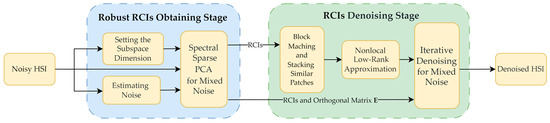
Figure 2.
Flowchart of the proposed RRGNLA method for HSI mixed denoising.
4. Experiments
In this section, we performed experiments on both simulated and real HSI datasets. Through both visual quality comparison and quantitative evaluation, we demonstrated the effectiveness of the proposed RRGNLA method for HSI mixed denoising. Nine methods that represent the most advanced techniques for HSI denoising were selected for comparison, i.e., BM4D [46], LRMR [13], NGMeet [27], FastHyDe [24], GLF [25], SNLRSF [34], NS3R [32], HyWTNN [36], and DTSVD [47]. The parameters involved in these methods were set based on the references and then fine-tuned to achieve optimal denoising performance for the datasets. We normalized each band of HSIs before denoising. All experiments were conducted in MATLAB R2023a with Intel® Xeon® CPU E3-1230 and 16 GB memory (Lenovo, Xi’an, China).
4.1. Simulated Data Experiments
4.1.1. Simulated Datasets
In the simulated experiments, we selected two commonly used datasets with ground truth. The first dataset utilized is the Washington DC Mall (WDC, http://engineering.purdue.edu/biehl/MultiSpec/hyperspectral.html, accessed on 28 October 2022), which consists of 1208 × 307 pixels and encompasses 210 spectral bands. In this paper, we select sub-images of size 256 × 256 × 191 for our experiments. The second dataset utilized is the Pavia University (PaU, http://www.ehu.es/ccwintco/index.php, accessed on 6 November 2022) dataset, which comprises images with a resolution of 1400 × 512 pixels and contains 102 spectral bands. In this paper, we select sub-images of size 300 × 300 × 102 for our experiments. To simulate noisy HSI data, Gaussian noise, impulse noise, deadlines, and stripes are added to two HSI datasets in four cases:
- Case 1: Zero-mean Gaussian noise with different standard deviations is added to each band, and the standard deviation of each band is randomly selected in the range of [0.1–0.2].
- Case 2: The Gaussian noise is added to each band with the same as in Case 1. In addition, impulse noise with a density of 20% is added into 20 randomly selected bands.
- Case 3: The Gaussian noise and impulse noise are added with the same as in Case 2. In addition, deadlines with widths ranging from 1 to 3 are added into the 20 bands. Among these, 10 bands will be selected from those affected by impulse noise, while the remaining 10 bands will be randomly chosen from the other bands.
- Case 4: The Gaussian noise, impulse noise, and deadlines are added with the same as in Case 3. In addition, we selected 20 consecutive bands to add random stripes, ensuring that 10% of the columns in each band were contaminated.
4.1.2. Visual Quality Comparison
Here, we select representative denoising results to demonstrate the effectiveness of the proposed RRGNLA method. For the WDC dataset, Figure 3 and Figure 4 illustrate the denoised images of band 9 (in Case 3) and band 82 (in Case 4) by different denoising methods. At the same time, in order to facilitate a more effective visual quality comparison, we have highlighted the same subregion with red boxes in Figure 3 and Figure 4. Similarly, for the PaU dataset, Figure 5 and Figure 6 present the denoised images of band 17 (in Case 3) and band 88 (in Case 4) using different denoising methods.
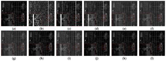
Figure 3.
Denoised images by different methods on the band 9 of the WDC dataset in Case 3. (a) Original, (b) noisy, (c) BM4D, (d) LRMR, (e) NGMeet, (f) FastHyDe, (g) GLF, (h) SNLRSF, (i) NS3R, (j) HyWTNN, (k) DTSVD, (l) RRGNLA.
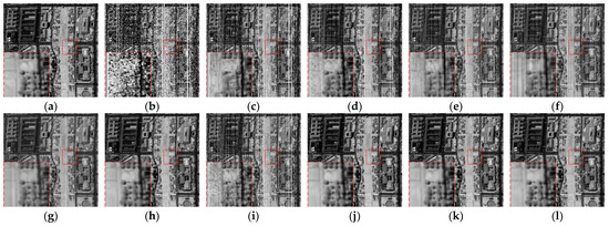
Figure 4.
Denoised images using different methods on the band 82 of the WDC dataset in Case 4. (a) Original, (b) noisy, (c) BM4D, (d) LRMR, (e) NGMeet, (f) FastHyDe, (g) GLF, (h) SNLRSF, (i) NS3R, (j) HyWTNN, (k) DTSVD, (l) RRGNLA.
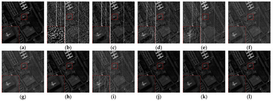
Figure 5.
Denoised images using different methods on the band 17 of the PaU dataset in Case 3. (a) Original, (b) noisy, (c) BM4D, (d) LRMR, (e) NGMeet, (f) FastHyDe, (g) GLF, (h) SNLRSF, (i) NS3R, (j) HyWTNN, (k) DTSVD, (l) RRGNLA.
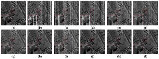
Figure 6.
Denoised images using different methods on the band 88 of the PaU dataset in Case 4. (a) Original, (b) noisy, (c) BM4D, (d) LRMR, (e) NGMeet, (f) FastHyDe, (g) GLF, (h) SNLRSF, (i) NS3R, (j) HyWTNN, (k) DTSVD, (l) RRGNLA.
From Figure 3, Figure 4, Figure 5 and Figure 6, it can be observed that our proposed RRGNLA method demonstrates effective denoising performance on both the WDC dataset and the PaU dataset. At the same time, we also observed that classic denoising methods, namely, BM4D and LRMR, show less efficacy in removing mixed noise. Although denoising methods based on NSR, such as GLF and SNLRSF, demonstrate good denoising results, our proposed RRGNLA method is able to recover the details of the hyperspectral images more effectively. This can be observed in the magnified sub-images in Figure 3, Figure 4, Figure 5 and Figure 6. Due to the lack of construction for RCIs in mixed noise circumstances, the denoising results of NS3R in our experiments were unsatisfactory. This also indicates that the robust RCIs we constructed played a role in removing mixed noise.
4.1.3. Quantitative Comparison
Five commonly used quantitative metrics are employed to evaluate the performance of various denoising methods. These include the mean peak signal-to-noise ratio (MPSNR), the mean structural similarity index (MSSIM) [48], and the mean feature similarity index (MFSIM) [49], all of which indicate better denoising results with higher values. Conversely, two metrics, namely, the erreur relative globale adimensionnelle de synthese (ERGAS) [50] and spectral angle mean (SAM) [51], signify improved denoising results with lower values. Meanwhile, in order to compare the denoising efficiency of different methods, we also present the computation time (in seconds). Table 1 and Table 2, respectively, summarize the quantitative evaluation results of different denoising methods in Cases 1–4 for the WDC dataset and the PaU dataset. Best and second results are highlighted in bold and underline, respectively.

Table 1.
Quantitative comparison results using different methods with the simulated Cases 1–4 on the WDC datasets.
Table 2.
Quantitative comparison results using different methods with the simulated Cases 1–4 on the PaU datasets.
From Table 1 and Table 2, it can be observed that the proposed RRGNLA method demonstrates optimal performance across most metrics, further underscoring the advanced capability of RRGNLA in effectively removing mixed noise. The proposed RRGNLA method also demonstrates competitive performance in terms of denoising efficiency. In the experiments conducted on two simulated datasets, its computation time consistently ranks second. In all simulated experiments, FastHyDe has the shortest computation time; however, its denoising performance is only average. For example, in Case 4 of the WDC dataset, while FastHyDe is more efficient in terms of computation time than RRGNLA, its MPSNR value is nearly 4 dB lower than that of RRGNLA. The NS3R employs refinement in the denoising process, causing a slightly longer computation time than RRGNLA. The SNLRSF outperforms RRGNLA in several metrics on the PaU dataset. However, SNLRSF exhibits poor performance in terms of denoising efficiency. For example, in Case 4 of the PaU dataset, the computation time of RRGNLA is nearly 40 times faster than that of SNLRSF. Although the HyWTNN and the DTSVD demonstrate competitive denoising performance on the PaC dataset compared to the proposed RRGNLA method, their performance on the WDC dataset is only average. This further demonstrates the strong adaptability of the proposed RRGNLA method across different datasets. To more intuitively compare the denoising results of different methods, we have also plotted the PSNR and SSIM values for the WDC dataset in Case 3 and the PaU dataset in Case 4, as shown in Figure 7.
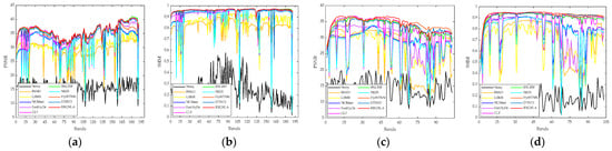
Figure 7.
PSNR and SSIM values of each band for the WDC and the PaU datasets. (a,b) The WDC dataset in Case 3. (c,d) The PaU dataset in Case 4.
4.2. Real Data Experiments
4.2.1. Real HSI Datasets
Denoising real HSI datasets presents a greater challenge due to the complexity of the noise circumstance. Here, we have selected two commonly used real HSI datasets, including the Indian Pines dataset (India, http://www.ehu.eus/ccwintco/index.php, accessed on 1 May 2023) and the Urban dataset (Urban, http://www.erdc.usace.army.mil/Media/Fact-Sheets/Fact-Sheet-Article-View/Article/610433/hypercube/, accessed on 17 July 2023). The Indian Pines dataset consists of 145 × 145 pixels and encompasses 220 spectral bands. The Urban dataset comprises 307 × 307 pixels and includes 210 spectral bands. During the experiments, we used the HySime algorithm [42] to estimate the variance in the real HSI datasets and set an appropriate subspace dimension based on this noise variance.
4.2.2. Results Comparison
Here, we present the denoising results of the Indian and Urban datasets under different methods, as shown in Figure 8 and Figure 9 respectively. To better visualize the denoising results of the Indian dataset, we present a false color image composed of three band combinations (R:108, B:140, G:220) in Figure 8a. From Figure 8 and Figure 9, it can be readily observed that our proposed method not only demonstrates superior visual quality, but also retains more details compared to the other methods under comparison.
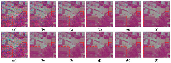
Figure 8.
Denoising results for Indian Pines dataset: (a) original false color image, (b) BM4D, (c) LRMR, (d) NGMeet, (e) FastHyDe, (f) GLF, (g) original false color image, (h) SNLRSF, (i) NS3R, (j) HyWTNN, (k) DTSVD, (l) RRGNLA.
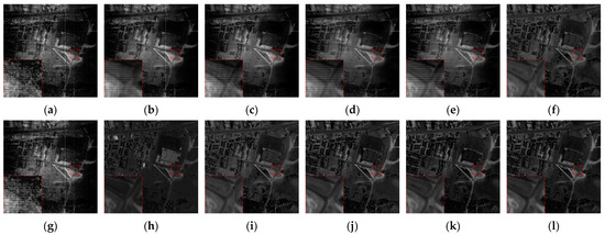
Figure 9.
Denoising results for Urban dataset: (a) original, (b) BM4D, (c) LRMR, (d) NGMeet, (e) FastHyDe, (f) GLF, (g) original, (h) SNLRSF, (i) NS3R, (j) HyWTNN, (k) DTSVD, (l) RRGNLA.
In addition, we have plotted the spectral signature curves of specific pixels under different denoising methods to compare their denoising performance, as illustrated in Figure 10 and Figure 11. It is not difficult to observe from Figure 10 and Figure 11 that the RRGNLA method we proposed is capable of effectively estimating the spectral signature values under both real HSI datasets. Finally, we present the computation times of different denoising methods on two real HSI datasets in Table 3. In two real HSI datasets, the RRGNLA method we proposed continues to demonstrate competitive denoising efficiency.
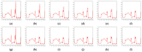
Figure 10.
Spectral signature curves on pixel point (10, 90) of the Indian dataset: (a) original, (b) BM4D, (c) LRMR, (d) NGMeet, (e) FastHyDe, (f) GLF, (g) original, (h) SNLRSF, (i) NS3R, (j) HyWTNN, (k) DTSVD, (l) RRGNLA.
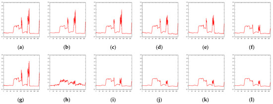
Figure 11.
Spectral signature curves on pixel point (10, 90) of the Urban dataset: (a) original, (b) BM4D, (c) LRMR, (d) NGMeet, (e) FastHyDe, (f) GLF, (g) original, (h) SNLRSF, (i) NS3R, (j) HyWTNN, (k) DTSVD, (l) RRGNLA.
Table 3.
Computation times of different denoising methods on two real HSI datasets.
4.3. Discussion
4.3.1. Parameters Setting
In this section, we analyze the parameter values required for conducting experiments with both simulated and real HSI datasets. In all experiments conducted to obtain robust RCIs, we set parameters and to 1 × 10⁻⁶ and 0.1, respectively, while the value of parameter was selected from the set {1 × 10⁻⁵, 2 × 10⁻⁵, 3 × 10⁻⁵, 4 × 10⁻⁵, 5 × 10⁻⁵}. In the low-rank approximation process, to enhance the computational efficiency of our proposed RRGNLA method, we select smaller 3D patch sizes and fewer similar patches. In all experiments, the values for l and s were set to 4 and 150, respectively. During the iterative denoising stage, we select and from the sets {0.05, 0.1, 0.2, 0.4, 0.6, 0.8} and {0.05, 0.1, 0.15, 0.2, 0.25, 0.3, 0.35, 0.4}, respectively, to adapt to different datasets and achieve better denoising results. The selection of the subspace dimension k is crucial to the denoising results. In simulated HSI dataset experiments, we select k from the set {3, 4, 5, 6, 7, 8, 9, 10}. The heavier the noise, the smaller the k we choose. In real HSI dataset experiments, we estimate the k using the HySime algorithm and subsequently fine-tune it.
4.3.2. Ablation Study
(1) Parameter sensitivity analysis: Here, we analyze the adjustable parameters in the proposed model involved in the RRGNLA, including the regularization parameter and subspace dimension k during the stage in which robust RCIs are obtained, as well as the regularization parameters and in the RCI denoising stage. We conducted tests on the PaU dataset and plotted the changes in the MPSNR values under different parameters, as shown in Figure 12. For the regularization parameter , the MPSNR values show little variation across all four cases for different values, indicating that the proposed RRGNLA method is not sensitive to this parameter. The optimal subspace dimension k (where the MPSNR value is maximized) decreases as the noise level increases. As shown in Figure 12b, in Case 1, the optimal subspace dimension is 4, whereas in Case 4, it is 3. For parameters and , we plot the 2D surface in Case 4, as shown in Figure 12c. The grid search over the two parameters intuitively reveals their impact on denoising performance.
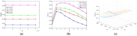
Figure 12.
Sensitivity analysis of different parameters on the PaU dataset: (a) MPSNR versus regularization parameter , (b) MPSNR versus number of subspace k, (c) MPSNR versus regularization parameters and in Case 4.
(2) Comparison of Different Methods for Obtaining RCIs: We compare three different methods for obtaining RCIs, that is, PCA (or SVD), SPCA in [32], and our method. Specifically, we denoise the RCIs obtained from the three methods using the WNNM low-rank regularizer. To ensure a fair comparison in our experiments, the subspace dimension k for all three methods was set to 5. Table 4 presents the quantitative evaluation results for the WDC and PaU datasets in Case 4. From Table 4, it can be observed that the RCIs constructed using our method exhibit strong robustness to mixed noise. Due to the lack of consideration for sparse noise, the RCIs obtained through the SPCA in [32] demonstrate average performance in mixed denoising. For instance, in the PaU dataset, its denoising performance even underperforms the RCIs constructed using PCA, as indicated by the MSISM and SAM metrics.
Table 4.
Comparison of denoising performance of RCIs constructed using different methods.
(3) Effectiveness of Robust RCIs and iterative denoising strategy: In this section, we compare the proposed RRGNLA method with three other methods: (1) without the robust RCIs guidance, denoted as NLA; (2) without iterative denoising strategy, denoted as RRG; (3) without norm constraints for sparse noise during the RCIs denoising stage, denoted as RRGN. Table 5 presents the comparison results of three different metrics on the WDC and PaU datasets. We can observe that the proposed RRGNLA method achieves the best quantitative results, indicating the effectiveness of robust RCIs guidance and iterative denoising strategy in enhancing denoising performance.
Table 5.
Quantitative comparison results of different methods on two simulated datasets.
4.3.3. Comparison with Deep Learning Methods
Recently, deep learning-based HSI denoising methods have garnered increased attention. Here, we additionally compare the proposed RRGNLA method with three state-of-the-art deep learning-based methods, including SDeCNN [52], FastHyMix [53], and MAC-Net [54]. The quantitative comparison results are shown in Table 6. From Table 6, it can be observed that the proposed RRGNLA method is competitive with deep learning-based methods. As the noise level increases, the proposed RRGNLA method exhibits greater robustness in denoising performance.
Table 6.
Quantitative comparison results of the proposed RRGNLA method and three deep learning-based methods on the WDC dataset.
4.3.4. Complexity and Convergence Analysis
In this section, we briefly analyze the computational complexity and convergence of the proposed RRGNLA method. Let m, n, and b represent the three dimensions of an HSI, and let k denote the subspace dimension. To simplify the description, we directly utilize the two-dimensional matrix form of the HSI data to analyze computational complexity. During the robust RCIs obtaining stage (see Algorithm 1), the computational complexity of solving Model (5) is determined using Equation (6). In Equation (6), the computational complexity of the three-dimensional tensor is , while the computational complexity of the soft-thresholding operator is . Since k is much smaller than b, the overall computational complexity of the robust RCI obtaining stage is .
During the RCIs denoising stage (see Algorithm 2), the computational complexity is mainly concentrated in the WNNM low-rank regularizer (determined using block matching and low-rank approximation) and the solution of Model (17).
- 1.
- Block Matching: Let denote the search window size; denotes the spatial size of the 3D patch. Calculating the similarity patch within a search window requires .
- 2.
- Low-Rank Approximation: The computational complexity of the low-rank approximation is determined using the SVD step. For a low-rank matrix of size , where s is the number of similar patches, the computational complexity of the SVD step is .
- 3.
- Solving Model (17): The computational complexity of solving Model (17) is determined using Equation (18). In Equation (18), the computational complexity for matrix operations is , and performing the soft-thresholding operation requires . We disregard the impact of k; therefore, the overall complexity of the iterative denoising process is .
In summary, for an HSI of size , the overall computational complexity of the RCI denoising stage is .
Additionally, to validate the convergence of the proposed RRGNLA method, we provide the convergence curves for different metrics on the WDC and PaU datasets in Case 3 and Case 4, as illustrated in Figure 13 and Figure 14, respectively. As the number of iterations increases, the changes in the values of MPSNR, MSSIM, and SAM tend to approach zero. This clearly demonstrates the convergence of the proposed RRGNLA method.
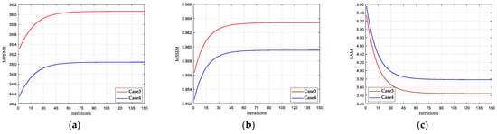
Figure 13.
Convergence analysis of three metrics on the WDC dataset: (a) MPSNR, (b) MSSIM, (c) SAM.
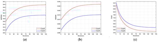
Figure 14.
Convergence analysis of three metrics on the PaU dataset: (a) MPSNR, (b) MSSIM, (c) SAM.
5. Conclusions
In this paper, we present a novel method based on NSR for the removal of mixed noise in HSI. The advanced denoising performance of this method is due to two main factors: (1) By utilizing an SPCA-based elastic net model to construct RCIs, the obtained RCIs better inherit the spatial structure of clean HSI. (2) The robust RCIs obtained are utilized as prior information for iterative denoising. Extensive comparative experiments and ablation studies demonstrate the effectiveness of constructing robust RCIs and employing them as prior information in an iterative denoiser for removing mixed noise from HSI. In the future, we will explore how to incorporate smooth prior information into the construction of robust RCIs to further enhance denoising performance.
Author Contributions
Conceptualization and methodology, J.S.; software, C.W.; validation, J.S.; formal analysis and investigation, F.H. and C.L.; resources, C.W.; data curation, Z.Y.; writing—original draft preparation, J.S.; writing—review and editing, J.S.; visualization, F.H.; supervision, B.G.; project administration and funding acquisition, B.G. All authors have read and agreed to the published version of the manuscript.
Funding
This research is supported financially by National Natural Science Foundation of China (Grant No. 62171341).
Data Availability Statement
The original contributions presented in the study are included in the article, further inquiries can be directed to the corresponding author.
Acknowledgments
We thank the editor and anonymous reviewers for their suggestions and comments, which have helped us to improve the quality of our work.
Conflicts of Interest
The authors declare no conflicts of interest.
Appendix A
In Appendix A, we provide a more detailed description of the optimization of the three subproblems in Model (5). For Equation (6), according to the study [43], we can solve it using the following lemma.
Lemma A1.
For and , the following optimization problem is presented:
can be solved using the soft-thresholding operator , which is defined as follows:
where denotes the sign function. Due to the similarity structure of Equations (6) and (A1), the solution to Equation (6) can be expressed as .
For Equation (7), we rewrite the Frobenius norm expansion as follows:
Given the variables S and , the minimization problem in Equation (A3) can be transformed into the following maximization problem:
where . We perform a singular value decomposition on A:
where denotes the diagonal matrix, U and V denote the left and right singular vectors of the SVD decomposition, respectively. The maximization problem in Equation (A4) is equivalent to the following maximization problem:
According to Appendix B in study [45], the orthogonality of E allows Equation (A6) to reach its maximum value when . Therefore, the closed-form solution of Equation (7) is .
For Equation (11), the proximal gradient method [32,45] is employed to optimize the variable S subject to elastic net regularization. Since Equation (11) shares the same structure as Equation (4.9) in study [45], we use as the proximal gradient for S. According to the discussion on unstructured sparsity in Appendix A of study [45], the problem in Equation (11) can be optimized using the scaled soft-thresholding operator, which corresponds to Equation (12). For a more detailed description of the scaled soft-thresholding operator, refer to Table 1 in Appendix A of study [45].
References
- Ghamisi, P.; Yokoya, N.; Li, J.; Liao, W.; Liu, S.; Plaza, J.; Rasti, B.; Plaza, A. Advances in hyperspectral image and signal processing: A comprehensive overview of the state of the art. IEEE Geosci. Remote Sens. Mag. 2017, 5, 37–78. [Google Scholar] [CrossRef]
- Peng, J.; Sun, W.; Li, H.-C.; Li, W.; Meng, X.; Ge, C.; Du, Q. Low-rank and sparse representation for hyperspectral image processing: A review. IEEE Geosci. Remote Sens. Mag. 2021, 10, 10–43. [Google Scholar] [CrossRef]
- Stuart, M.B.; McGonigle, A.J.; Willmott, J.R. Hyperspectral imaging in environmental monitoring: A review of recent developments and technological advances in compact field deployable systems. Sensors 2019, 19, 3071. [Google Scholar] [CrossRef] [PubMed]
- Goetz, A.F. Three decades of hyperspectral remote sensing of the Earth: A personal view. Remote Sens. Environ. 2009, 113, S5–S16. [Google Scholar] [CrossRef]
- Shimoni, M.; Haelterman, R.; Perneel, C. Hyperspectral imaging for military and security applications: Combining myriad processing and sensing techniques. IEEE Geosci. Remote Sens. Mag. 2019, 7, 101–117. [Google Scholar] [CrossRef]
- Zhang, Y.; Du, B.; Zhang, L.; Liu, T. Joint sparse representation and multitask learning for hyperspectral target detection. IEEE Trans. Geosci. Remote Sens. 2016, 55, 894–906. [Google Scholar] [CrossRef]
- Zeng, S.; Wang, Z.; Gao, C.; Kang, Z.; Feng, D. Hyperspectral image classification with global–local discriminant analysis and spatial–spectral context. IEEE J. Sel. Top. Appl. Earth Obs. Remote Sens. 2018, 11, 5005–5018. [Google Scholar] [CrossRef]
- Cao, X.; Yao, J.; Xu, Z.; Meng, D. Hyperspectral image classification with convolutional neural network and active learning. IEEE Trans. Geosci. Remote Sens. 2020, 58, 4604–4616. [Google Scholar] [CrossRef]
- Rasti, B.; Sveinsson, J.R.; Ulfarsson, M.O. Wavelet-based sparse reduced-rank regression for hyperspectral image restoration. IEEE Trans. Geosci. Remote Sens. 2014, 52, 6688–6698. [Google Scholar] [CrossRef]
- Zhao, Y.-Q.; Yang, J. Hyperspectral image denoising via sparse representation and low-rank constraint. IEEE Trans. Geosci. Remote Sens. 2014, 53, 296–308. [Google Scholar] [CrossRef]
- Dabov, K.; Foi, A.; Katkovnik, V.; Egiazarian, K. Image denoising by sparse 3-D transform-domain collaborative filtering. IEEE Trans. Image Process. 2007, 16, 2080–2095. [Google Scholar] [CrossRef] [PubMed]
- Gu, S.; Zhang, L.; Zuo, W.; Feng, X. Weighted Nuclear Norm Minimization with Application to Image Denoising. In Proceedings of the IEEE/CVF Conference on Computer Vision and Pattern Recognition (CVPR), Columbus, OH, USA, 24–27 June 2014; pp. 2862–2869. [Google Scholar]
- Zhang, H.; He, W.; Zhang, L.; Shen, H.; Yuan, Q. Hyperspectral image restoration using low-rank matrix recovery. IEEE Trans. Geosci. Remote Sens. 2013, 52, 4729–4743. [Google Scholar] [CrossRef]
- Lu, T.; Li, S.; Fang, L.; Ma, Y.; Benediktsson, J.A. Spectral–spatial adaptive sparse representation for hyperspectral image denoising. IEEE Trans. Geosci. Remote Sens. 2015, 54, 373–385. [Google Scholar] [CrossRef]
- Xue, J.; Zhao, Y.; Liao, W.; Kong, S.G. Joint spatial and spectral low-rank regularization for hyperspectral image denoising. IEEE Trans. Geosci. Remote Sens. 2017, 56, 1940–1958. [Google Scholar] [CrossRef]
- Fan, H.; Chen, Y.; Guo, Y.; Zhang, H.; Kuang, G. Hyperspectral image restoration using low-rank tensor recovery. IEEE J. Sel. Top. Appl. Earth Obs. Remote Sens. 2017, 10, 4589–4604. [Google Scholar] [CrossRef]
- Huang, Z.; Li, S.; Fang, L.; Li, H.; Benediktsson, J.A. Hyperspectral image denoising with group sparse and low-rank tensor decomposition. IEEE Access 2017, 6, 1380–1390. [Google Scholar] [CrossRef]
- Xue, J.; Zhao, Y.; Huang, S.; Liao, W.; Chan, J.C.-W.; Kong, S.G. Multilayer sparsity-based tensor decomposition for low-rank tensor completion. IEEE Trans. Neural Netw. Learn. Syst. 2021, 33, 6916–6930. [Google Scholar] [CrossRef]
- Fan, H.; Li, C.; Guo, Y.; Kuang, G.; Ma, J. Spatial–spectral total variation regularized low-rank tensor decomposition for hyperspectral image denoising. IEEE Trans. Geosci. Remote Sens. 2018, 56, 6196–6213. [Google Scholar] [CrossRef]
- Peng, J.; Xie, Q.; Zhao, Q.; Wang, Y.; Yee, L.; Meng, D. Enhanced 3DTV regularization and its applications on HSI denoising and compressed sensing. IEEE Trans. Image Process. 2020, 29, 7889–7903. [Google Scholar] [CrossRef]
- Sarkar, S.; Sahay, R.R. A non-local superpatch-based algorithm exploiting low rank prior for restoration of hyperspectral images. IEEE Trans. Geosci. Remote Sens. 2021, 30, 6335–6348. [Google Scholar] [CrossRef]
- Xie, Q.; Zhao, Q.; Meng, D.; Xu, Z. Kronecker-basis-representation based tensor sparsity and its applications to tensor recovery. IEEE Trans. Pattern Anal. Mach. Intell. 2017, 40, 1888–1902. [Google Scholar] [CrossRef] [PubMed]
- Xue, J.; Zhao, Y.; Liao, W.; Chan, J.C.-W. Nonlocal low-rank regularized tensor decomposition for hyperspectral image denoising. IEEE Trans. Geosci. Remote Sens. 2019, 57, 5174–5189. [Google Scholar] [CrossRef]
- Zhuang, L.; Bioucas-Dias, J.M. Fast hyperspectral image denoising and inpainting based on low-rank and sparse representations. IEEE J. Sel. Top. Appl. Earth Obs. Remote Sens. 2018, 11, 730–742. [Google Scholar] [CrossRef]
- Zhuang, L.; Fu, X.; Ng, M.K.; Bioucas-Dias, J.M. Hyperspectral image denoising based on global and nonlocal low-rank factorizations. IEEE Trans. Geosci. Remote Sens. 2021, 59, 10438–10454. [Google Scholar] [CrossRef]
- Lin, J.; Huang, T.-Z.; Zhao, X.-L.; Jiang, T.-X.; Zhuang, L. A tensor subspace representation-based method for hyperspectral image denoising. IEEE Trans. Geosci. Remote Sens. 2020, 59, 7739–7757. [Google Scholar] [CrossRef]
- He, W.; Yao, Q.; Li, C.; Yokoya, N.; Zhao, Q.; Zhang, H.; Zhang, L. Non-local meets global: An iterative paradigm for hyperspectral image restoration. IEEE Trans. Pattern Anal. Mach. Intell. 2020, 44, 2089–2107. [Google Scholar] [CrossRef]
- Xu, S.; Cao, X.; Peng, J.; Ke, Q.; Ma, C.; Meng, D. Hyperspectral image denoising by asymmetric noise modeling. IEEE Trans. Geosci. Remote Sens. 2022, 60, 5545214. [Google Scholar] [CrossRef]
- Su, X.; Zhang, Z.; Yang, F. Fast hyperspectral image denoising and destriping method based on graph Laplacian regularization. IEEE Trans. Geosci. Remote Sens. 2023, 61, 5511214. [Google Scholar] [CrossRef]
- Chen, Y.; Zeng, J.; He, W.; Zhao, X.-L.; Jiang, T.-X.; Huang, Q. Fast Large-Scale Hyperspectral Image Denoising via Non-Iterative Low-Rank Subspace Representation. IEEE Trans. Geosci. Remote Sens. 2024, 33, 1211–1226. [Google Scholar]
- Ashraf, M.; Chen, L.; Zhou, X.; Rakha, M.A. A Joint Architecture of Mixed-Attention Transformer and Octave Module for Hyperspectral Image Denoising. IEEE J. Sel. Top. Appl. Earth Obs. Remote Sens. 2024, 17, 4331–4349. [Google Scholar] [CrossRef]
- Wang, H.; Peng, J.; Cao, X.; Wang, J.; Zhao, Q.; Meng, D. Hyperspectral image denoising via nonlocal spectral sparse subspace representation. IEEE J. Sel. Top. Appl. Earth Obs. Remote Sens. 2023, 16, 5189–5203. [Google Scholar] [CrossRef]
- Sun, L.; Jeon, B.; Soomro, B.N.; Zheng, Y.; Wu, Z.; Xiao, L. Fast superpixel based subspace low rank learning method for hyperspectral denoising. IEEE Access 2018, 6, 12031–12043. [Google Scholar] [CrossRef]
- Cao, C.; Yu, J.; Zhou, C.; Hu, K.; Xiao, F.; Gao, X. Hyperspectral image denoising via subspace-based nonlocal low-rank and sparse factorization. IEEE J. Sel. Top. Appl. Earth Obs. Remote Sens. 2019, 12, 973–988. [Google Scholar] [CrossRef]
- Zheng, Y.-B.; Huang, T.-Z.; Zhao, X.-L.; Chen, Y.; He, W. Double-factor-regularized low-rank tensor factorization for mixed noise removal in hyperspectral image. IEEE Trans. Geosci. Remote Sens. 2020, 58, 8450–8464. [Google Scholar] [CrossRef]
- He, C.; Cao, Q.; Xu, Y.; Sun, L.; Wu, Z.; Wei, Z. Weighted order-p tensor nuclear norm minimization and its application to hyperspectral image mixed denoising. IEEE Geosci. Remote Sens. Lett. 2023, 20, 5510505. [Google Scholar] [CrossRef]
- Fu, X.; Guo, Y.; Xu, M.; Jia, S. Hyperspectral image denoising via robust subspace estimation and group sparsity constraint. IEEE Trans. Geosci. Remote Sens. 2023, 61, 5512716. [Google Scholar] [CrossRef]
- Li, M.; Liu, J.; Fu, Y.; Zhang, Y.; Dou, D. Spectral Enhanced Rectangle Transformer for Hyperspectral Image Denoising. In Proceedings of the IEEE/CVF Conference on Computer Vision and Pattern Recognition (CVPR), Los Angeles, CA, USA, 24–27 June 2023; pp. 5805–5814. [Google Scholar]
- He, C.; Sun, L.; Huang, W.; Zhang, J.; Zheng, Y.; Jeon, B. TSLRLN: Tensor subspace low-rank learning with non-local prior for hyperspectral image mixed denoising. Signal Process. 2021, 184, 108060. [Google Scholar] [CrossRef]
- Zhang, Q.; Zheng, Y.; Yuan, Q.; Song, M.; Yu, H.; Xiao, Y. Hyperspectral image denoising: From model-driven, data-driven, to model-data-driven. IEEE Trans. Neural Netw. Learn. Syst. 2023, 35, 13143–13163. [Google Scholar] [CrossRef]
- Yi, L.; Zhao, Q.; Xu, Z. Hyperspectral Image Denoising by Pixel-Wise Noise Modeling and TV-Oriented Deep Image Prior. Remote Sens. 2024, 16, 2694. [Google Scholar] [CrossRef]
- Bioucas-Dias, J.M.; Nascimento, J.M. Hyperspectral subspace identification. IEEE Trans. Geosci. Remote Sens. 2008, 46, 2435–2445. [Google Scholar] [CrossRef]
- Donoho, D.L. De-noising by soft-thresholding. IEEE Trans. Inf. Theory 1995, 41, 613–627. [Google Scholar] [CrossRef]
- Gower, J.C.; Dijksterhuis, G.B. Procrustes Problems; OUP: Oxford, UK, 2004; Volume 30. [Google Scholar]
- Erichson, N.B.; Zheng, P.; Manohar, K.; Brunton, S.L.; Kutz, J.N.; Aravkin, A.Y. Sparse principal component analysis via variable projection. SIAM J. Appl. Math. 2020, 80, 977–1002. [Google Scholar] [CrossRef]
- Maggioni, M.; Katkovnik, V.; Egiazarian, K.; Foi, A. Nonlocal transform-domain filter for volumetric data denoising and reconstruction. IEEE Trans. Image Process. 2012, 22, 119–133. [Google Scholar] [CrossRef]
- He, C.; Xu, Y.; Wu, Z.; Zheng, S.; Wei, Z. Multi-Dimensional Visual Data Restoration: Uncovering the Global Discrepancy in Transformed High-Order Tensor Singular Values. IEEE Trans. Image Process. 2024, 33, 6409–6424. [Google Scholar] [CrossRef]
- Wang, Z.; Bovik, A.C.; Sheikh, H.R.; Simoncelli, E.P. Image quality assessment: From error visibility to structural similarity. IEEE Trans. Image Process. 2004, 13, 600–612. [Google Scholar] [CrossRef]
- Zhang, L.; Zhang, L.; Mou, X.; Zhang, D. FSIM: A feature similarity index for image quality assessment. IEEE Trans. Image Process. 2011, 20, 2378–2386. [Google Scholar] [CrossRef]
- Wald, L. Data Fusion: Definitions and Architectures: Fusion of Images of Different Spatial Resolutions; Presses des Mines: Paris, France, 2002. [Google Scholar]
- He, W.; Zhang, H.; Zhang, L.; Shen, H. Total-variation-regularized low-rank matrix factorization for hyperspectral image restoration. IEEE Trans. Geosci. Remote Sens. 2015, 54, 178–188. [Google Scholar] [CrossRef]
- Maffei, A.; Haut, J.M.; Paoletti, M.E.; Plaza, J.; Bruzzone, L.; Plaza, A. A single model CNN for hyperspectral image denoising. IEEE Trans. Geosci. Remote Sens. 2019, 58, 2516–2529. [Google Scholar] [CrossRef]
- Zhuang, L.; Ng, M.K. FastHyMix: Fast and parameter-free hyperspectral image mixed noise removal. IEEE Trans. Neural Netw. Learn. Syst. 2021, 34, 4702–4716. [Google Scholar] [CrossRef]
- Xiong, F.; Zhou, J.; Zhao, Q.; Lu, J.; Qian, Y. MAC-Net: Model-aided nonlocal neural network for hyperspectral image denoising. IEEE Trans. Geosci. Remote Sens. 2021, 60, 5519414. [Google Scholar] [CrossRef]
Disclaimer/Publisher’s Note: The statements, opinions and data contained in all publications are solely those of the individual author(s) and contributor(s) and not of MDPI and/or the editor(s). MDPI and/or the editor(s) disclaim responsibility for any injury to people or property resulting from any ideas, methods, instructions or products referred to in the content. |
© 2025 by the authors. Licensee MDPI, Basel, Switzerland. This article is an open access article distributed under the terms and conditions of the Creative Commons Attribution (CC BY) license (https://creativecommons.org/licenses/by/4.0/).