The Improved MNSPI Method for MODIS Surface Reflectance Data Small-Area Restoration

Abstract

Low-resolution satellites, due to their wide coverage and fast data acquisition, are commonly used in large-scale studies. However, these optical remote sensing data are often limited by weather conditions and sensor system issues during acquisition, which leads to missing information. For example, MODIS data, as a typical representative of low-resolution satellites, often encounter issues of small-region data loss, which corresponds to a large area on the surface of the earth due to the relatively large spatial scale of the pixels, thereby limiting the high-quality application of the data, especially in building datasets for deep learning. Currently, most missing data restoration methods are designed for medium-resolution data. However, low-resolution satellite data pose greater challenges due to the severe mixed-pixel problem and loss of texture features, leading to suboptimal restoration results. Even MNSPI, a typical method for restoring missing data based on similar pixels, is not exempt from these limitations. Therefore, this study integrates four-temporal phase characteristic information into the existing MNSPI algorithm. By comprehensively utilizing temporal–spatial–spectral information, we propose an algorithm for restoring small missing regions. Experiments were conducted under two scenarios: areas with complex surface types and areas with homogeneous surface types. Both simulated and real missing data cases were tested. The results demonstrate that the proposed algorithm outperforms the comparison methods across all evaluation metrics. Notably, we statistically analyzed the optimal restoration range of the algorithm in cases where similar pixels were identified. Specifically, the algorithm performs optimally when restoring regions with connected pixel areas smaller than 1936 pixels, corresponding to approximately 484 km² of missing surface area. Additionally, we applied the proposed algorithm to global surface reflectance data restoration, further validating its practicality and feasibility for large-scale application studies.

1. Introduction

Optical remote sensing data, as a primary source for surface observations, offer extensive coverage and rich spectral information [1,2,3,4]. Low-resolution satellites feature wide swath widths and fast data acquisition speeds, making them suitable for large-scale studies. In particular, the Moderate Resolution Imaging Spectroradiometer (MODIS), a representative of medium to low spatial resolution satellites, provides global scale surface observation data at spatial resolutions of 250 m, 500 m, and 1000 m, demonstrating significant advantages in global-scale Earth science research [5]. However, the application of MODIS surface reflectance products is often constrained by data quality issues, especially data loss caused by clouds, cloud shadows, and invalid pixels, which severely limit the accuracy and continuity of data analysis [6,7,8,9,10], thereby impacting downstream research tasks [11]. Additionally, due to the relatively large spatial scale of individual pixels in low-resolution satellites, missing regions composed of single or a few pixels are common. Drawing from the definition of small objects in object detection [12], we preliminarily define missing regions with fewer than 1024 pixels as small missing regions. When constructing deep learning datasets, assuming the use of standard 256 × 256 pixel remote sensing image patches, even such small-sized images correspond to a ground area of approximately 16,384 km², roughly the size of Beijing, where obtaining entirely cloud-free image patches remains challenging [13,14,15,16]. As shown in Figure 1a,c,d, the missing regions within 256 × 256-sized areas across different global regions exhibit a small region missing problem of approximately 10%. Furthermore, a statistical analysis of missing regions in the Tibetan Plateau reveals that over 70,000 missing regions contain fewer than 500 pixels, as indicated by the results in Figure 1b, highlighting the widespread nature of small regions missing. Such missing data pose challenges in constructing datasets for tasks like image segmentation [17] and image fusion [18], reducing model training effectiveness and generalization capability. Moreover, directly applying large-region restoration methods, while feasible, demands substantial computational resources and processing time. Therefore, to ensure data accuracy and the reliability of analytical results, developing specialized data reconstruction methods for missing small regions is particularly crucial.

Surface reflectance data, as a fundamental optical remote sensing product, have been widely applied in various fields such as urban development, disaster assessment, vegetation monitoring, and environmental change detection [19,20,21,22]. Over the past decades, researchers have proposed numerous methods to restore missing regions in MODIS data products. With the continuous advancement of deep learning in remote sensing, many studies have leveraged complex neural networks to automatically learn image features to restore missing regions [23,24,25,26,27,28,29]. However, the small region missing problem unique to MODIS data presents challenges in constructing diverse-scale deep learning datasets, which limits the ability of models to capture contextual information and subtle spatio-temporal variation patterns. To address this issue, many studies have considered first restoring small missing regions to increase the number of samples [30,31]. Therefore, this study adopts traditional image restoration methods and categorizes them into three types: spatial information-based methods, temporal information-based methods, and spatio-temporal information-based methods.

Reconstruction methods based on spatial information do not require additional auxiliary information; they fully utilize the effective global or local information within the target image to restore missing regions [32]. The most commonly used traditional methods include interpolation techniques, such as kriging interpolation [33,34,35], spline function interpolation [36], and inverse distance weighting interpolation [37]. These methods can achieve good restoration results in cases of small missing regions or areas with regular textures, but the reconstruction accuracy cannot be guaranteed for large missing areas or boundaries between different surfaces.

Reconstruction methods based on temporal information leverage images captured at the same location over different times as auxiliary data to restore missing areas. By utilizing the characteristic that land cover types remain unchanged over short periods, some approaches directly fill missing regions using adjacent temporal images [38]. However, methods relying on single auxiliary images often provide insufficient information, resulting in suboptimal restoration outcomes. To address these limitations, many researchers have adopted time-series data for restoration purposes [39,40]. While time-series data offer richer temporal information for improved restoration accuracy, their application in reconstructing large-scale missing regions requires substantial amounts of data, which in turn demands higher computational performance.

Reconstruction methods based on spatio-temporal information utilize the spatial, spectral, and temporal information of remote sensing images to restore missing regions. Based on the source of the data used, these methods can be categorized into heterogeneous-source and homogeneous-source approaches. Reconstruction methods based on heterogeneous-source data achieve restoration by integrating data from multiple sensors. A common approach is the fusion of Landsat and MODIS images to generate cloud-free images [41,42]. However, these methods require preprocessing steps such as image registration and image fusion, increasing algorithmic complexity. Reconstruction methods based on homogeneous-source data use the same sensor’s data for restoration. One approach employs spatio-temporal joint interpolation using time-series data [43,44]. However, due to the large data volume and high computational demands, this method is not suitable for large-scale applications. Another approach employs neighborhood similarity for restoration, characterized by low data requirements and effective results. The most notable example is the Modified Neighborhood Similar Pixel Interpolator (MNSPI) algorithm [45], an improvement upon the Neighborhood Similar Pixel Interpolator (NSPI) method [46]. Widely used in optical remote sensing image restoration, MNSPI identifies the most similar neighboring pixels within a specified range to restore missing data, dynamically adjusting the search window size to enhance restoration efficiency and quality. Due to its simplicity, ease of use, and strong performance, the MNSPI algorithm has been extensively applied, particularly in medium-resolution satellite data such as Landsat. However, when applied to MODIS data restoration, despite MNSPI achieving good results for small missing regions, the lower spatial resolution of MODIS leads to a loss of image details and texture features. Moreover, the mixed pixel problem becomes more severe [47], and using only a single auxiliary temporal phase is insufficient to accurately predict missing pixel values, ultimately reducing the effectiveness of the restoration.

The more severe issue of mixed pixels in MODIS data exacerbates the poor performance of the MNSPI algorithm in the application of MODIS data restoration [25]. In this paper, we leverage the characteristic of rapid data acquisition in MODIS, combining it with the restoration method for medium spatial resolution images and MODIS multi-temporal phase features, to propose a small area restoration algorithm. This algorithm, based on four-temporal phase features, utilizes the similarity between the target image and auxiliary images to repair missing areas. The main contributions of our work are summarized as follows:

• To address the limitations of the MNSPI algorithm in MODIS data, this study improves the MNSPI algorithm by leveraging the stability and invariance of land cover over short periods. The auxiliary information includes adjacent temporal phases before and after the missing phase, as well as data from the same period in the previous and following years. Based on the spectral similarity characteristics of the temporal information, different weights are assigned to the auxiliary temporal phases, and a comprehensive use of spatial–temporal–spectral information is made to achieve the reconstruction of missing MODIS data.
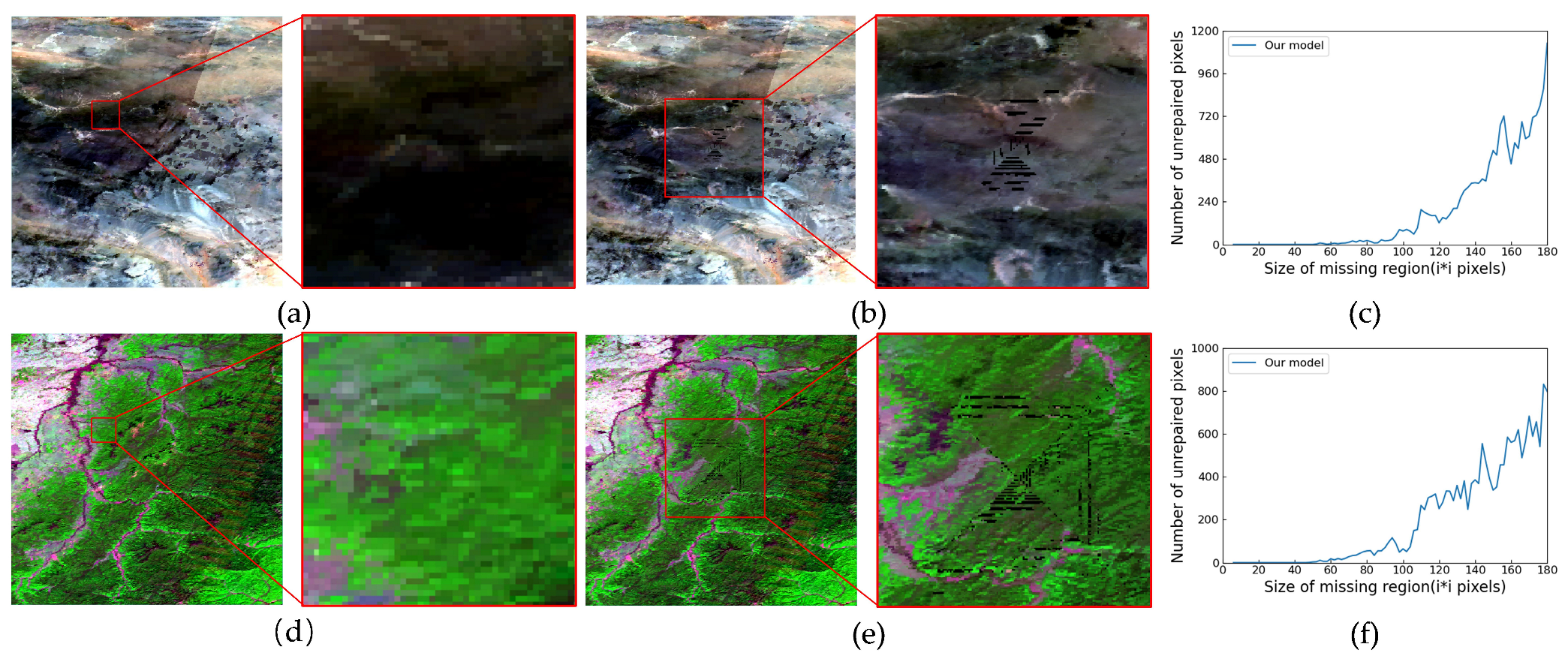
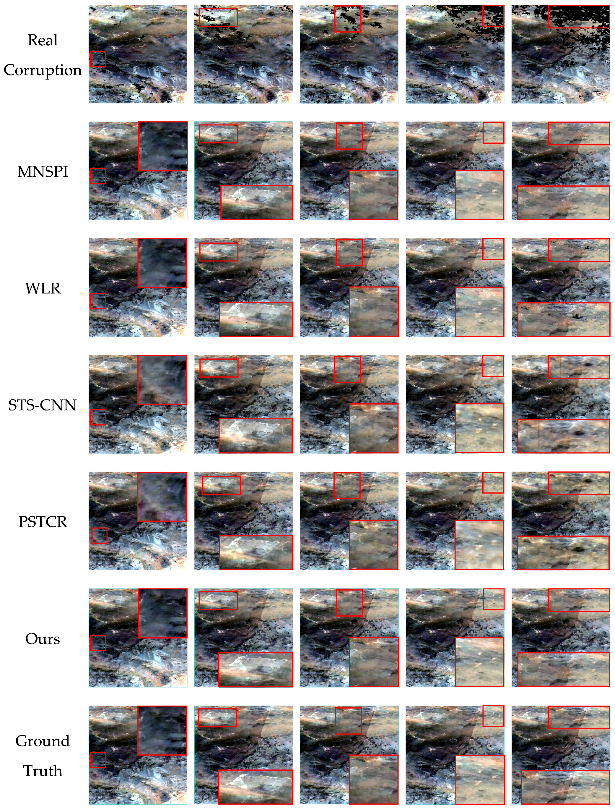
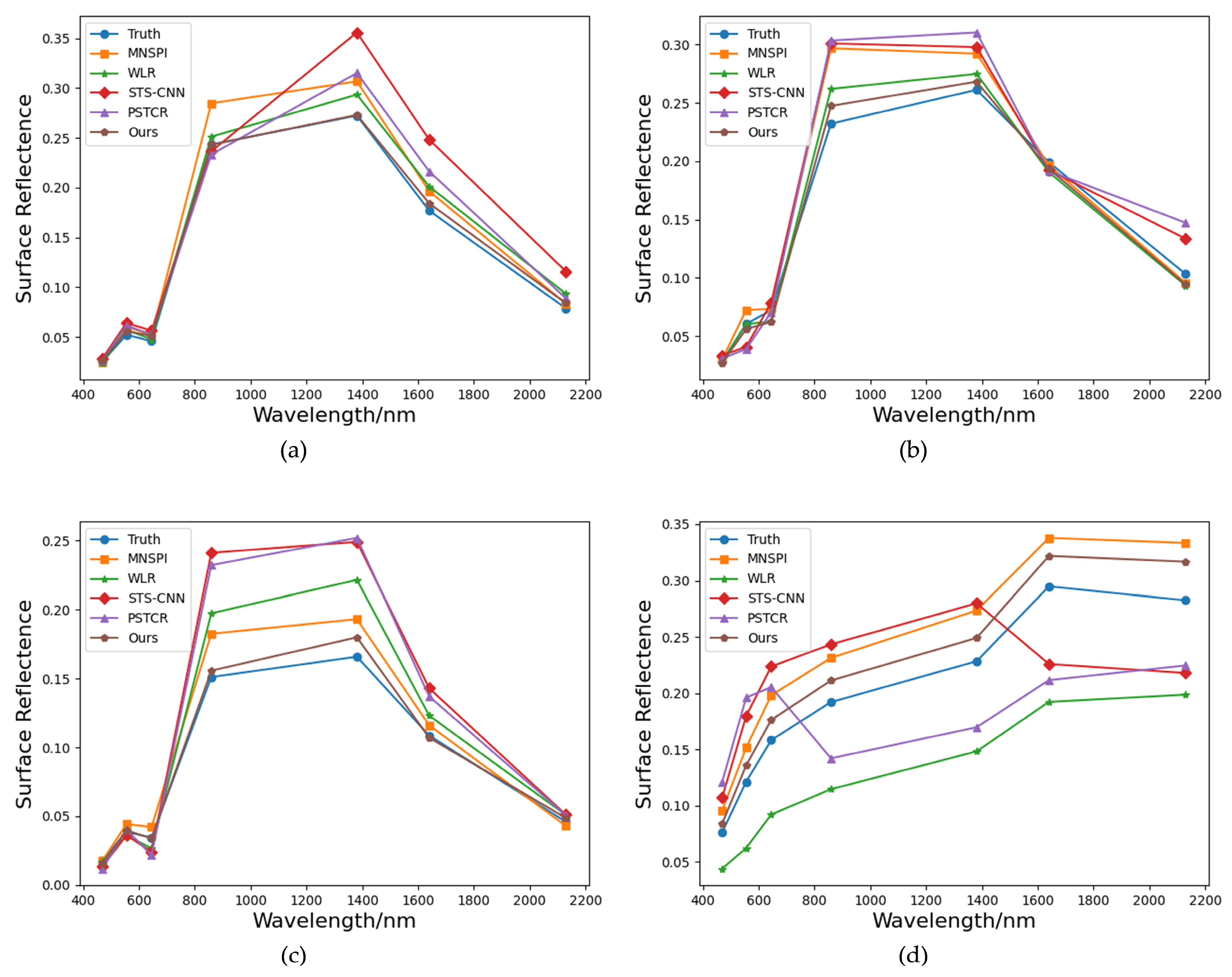
• To ensure the algorithm’s broad adaptability and reliability in handling diverse missing scenarios in practical applications, this study designs experiments with rectangular missing regions of different sizes. Simulated missing and real missing experiments are conducted in two scenarios with varying surface complexities. The experimental results show that the proposed method demonstrates strong robustness across different surface complexities, effectively restoring missing image regions. Additionally, this method outperforms the comparison algorithms in both qualitative and quantitative results. Moreover, to address the issue in existing algorithms where restoration effectiveness declines as the missing region expands, this study explicitly defines the optimal restoration range of the proposed method, specifically for small missing regions. This provides clear guidance for the practical application of the algorithm, ensuring more accurate reconstruction results across various missing scenarios.
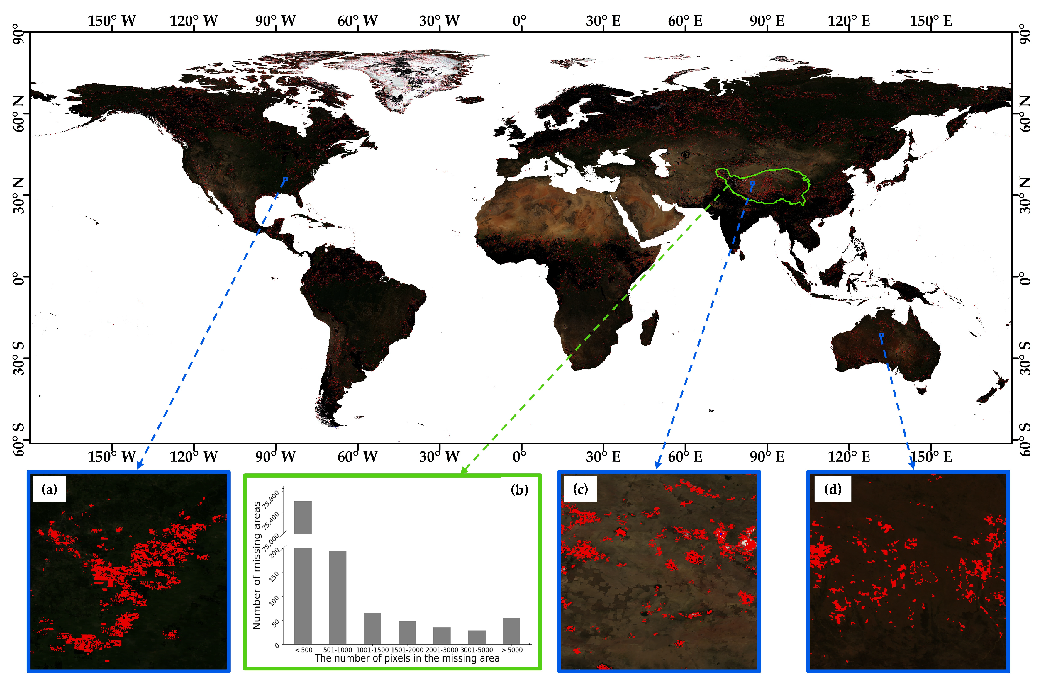
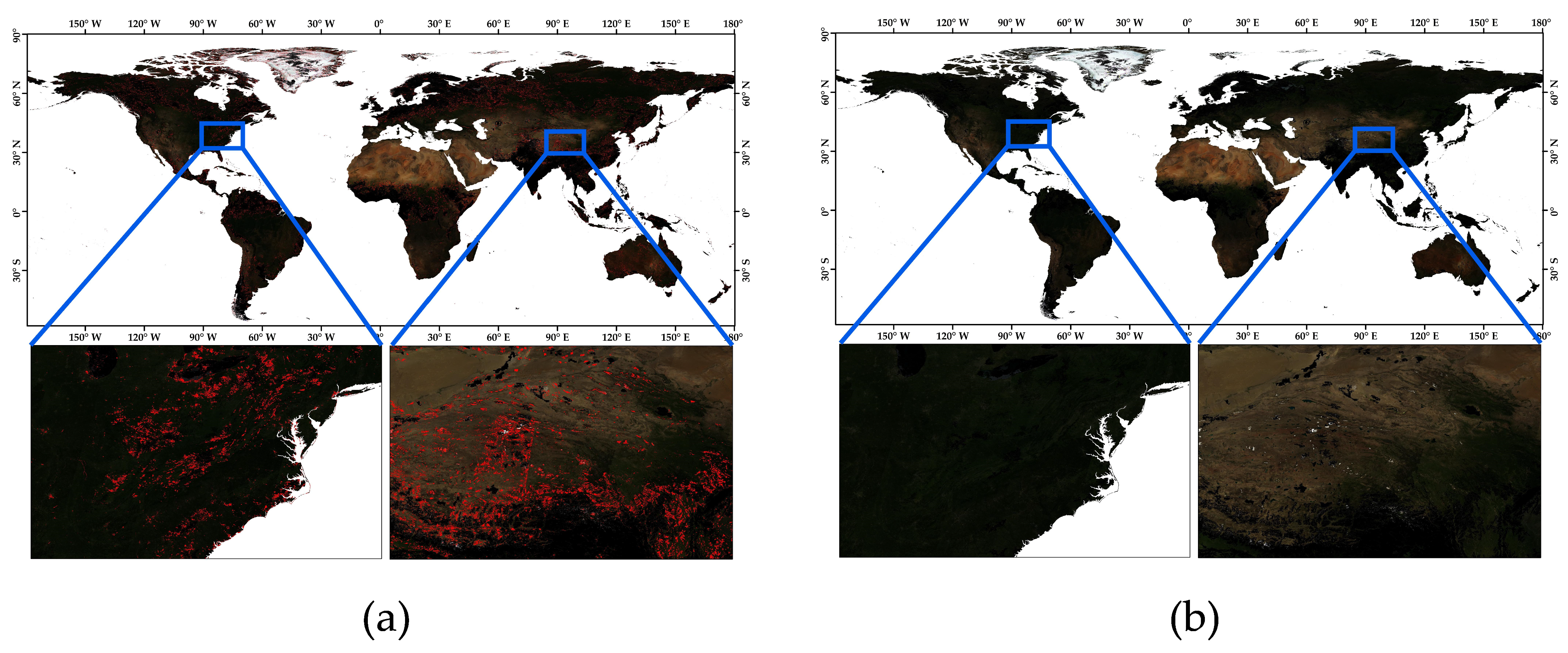
• To validate the algorithm’s reliability across different geographic regions, climate conditions, and land cover types, we apply the proposed algorithm to the global MODIS data restoration. The experimental results show that the method effectively restores small missing region data and maintains high reconstruction accuracy under diverse environmental conditions.

The structure of this paper is as follows: Section 2 introduces our proposed algorithm, including our improved algorithm framework and algorithm details. Section 3 describes the data used in this paper and the preprocessing work. Section 4 presents simulated data experiments and real data experiments to demonstrate the superiority of the improved method, along with the global application of the proposed algorithm. Finally, Section 5 summarizes the conclusions of this paper.

2. Methods

2.1. Overal Framework

Using the spectral similarity between pixels, the IMNSPI algorithm restores missing regions, but its performance is limited by the precision of low-resolution satellite data. To address this, this study utilizes the characteristics of short-term land surface stability and invariance, incorporating adjacent temporal phases before and after the target phase, as well as data from the same period in the preceding and following years, as auxiliary information. By integrating four-temporal phase information and adaptively assigning weights based on the spectral similarity between auxiliary phases and the target image, the proposed method achieves higher reconstruction accuracy. The overall structure of the proposed algorithm is shown in Figure 2, consisting of three main components: the input image, the reconstruction of missing regions, and the output reconstructed image. In the reconstruction phase, the first step is to calculate the spectral similarity between the auxiliary data and the image to be restored. If the similarity meets the required threshold, the temporal phase contributes to the subsequent restoration; otherwise, it does not. Next, neighboring pixels with similar spectral properties are searched around the missing pixels as similar pixels. Then, weights are assigned to similar pixels in each temporal phase based on their spectral values and spatial distances, and the spectral–spatial prediction values are calculated for each temporal phase. The average of these prediction values is taken to obtain a more accurate spectral–spatial prediction value. Additionally, based on the maximum spectral similarity of each temporal phase, different weights are assigned to each temporal phase. Using these weights, the spectral–temporal prediction values are calculated. Finally, by integrating the spectral–spatial prediction values and the spectral–temporal prediction values, the spatial–temporal–spectral prediction value is obtained, leading to more accurate reconstruction results.

2.2. MNSPI

The MNSPI method leverages the property that similar land cover types exhibit similar spectral characteristics to predict the spectral value of the target pixel from adjacent similar pixels, thereby achieving the restoration of missing areas in the image. It further accounts for the varying degrees of influence that different similar pixels exert on the target pixel, evaluating these influences through weighted assessments from both spatial and spectral dimensions [45]. Equations (1) and (2) represent the initial predictions based on the spectral–spatial distance and spectral–temporal distance, respectively:

$$L_{1,t}\left(x,y,b\right)=\sum _{i=1}^N{W}_i\times L_t\left(x_i,y_i,b\right)$$

(1)

$$L_{2,t}\left(x,y,b\right)=L_{t_n}\left(x,y,b\right)+\sum _{i=1}^N{W}_i\times (L_t\left(x_i,y_i,b\right)-L_{t_n}\left(x_i,y_i,b\right)$$

(2)

where $i$ denotes the $i$-th similar pixel; $t$ represents the target temporal image to be restored; $t_n$ refers to the $n$-th temporal auxiliary image; $\left(x_i,y_i\right)$ is the coordinate location of the $i$-th similar pixel in the image; $b$ represents the spectral band; $L_t\left(x_i,y_i,b\right)$ denotes the value of the $i$-th similar pixel at location $\left(x_i,y_i\right)$ for band $b$ at time $t$; $L_{t_n}\left(x_i,y_i,b\right)$ represents the value of the $i$-th similar pixel at location $\left(x_i,y_i\right)$ for band $b$ at time $t_n$; $L_{1,t}\left(x,y,b\right)$ represents the prediction value for the missing pixel at location $\left(x,y\right)$ in band $b$ at time $t$, based on the spectral–spatial distance; $L_{2,t}\left(x,y,b\right)$ denotes the prediction value based on the spectral–temporal distance; $N$ represents the total number of similar pixels; $W_i$ is the spatial information weight of the $i$-th similar pixel, derived from the normalized spatial distance $D_i^{*}$ and spectral distance ${RMSD}_i^{*}$, as defined in Equation (3).

$$W_i={\displaystyle \frac{\raisebox{1ex}{$1$}\!\left/ \!\raisebox{-1ex}{$\left(D_i^{*} \times {RMSD}_i^{*}\right)$}\right.}{{\sum }_{i=1}^N\left(\raisebox{1ex}{$1$}\!\left/ \!\raisebox{-1ex}{$\left(D_i^{*} \times {RMSD}_i^{*}\right)$}\right.\right)}}$$

(3)

where the spatial distance $D_i$ and spectral distance ${RMSD}_i$ are calculated using Equations (4) and (6), respectively. Due to the potentially large variations in spatial distance between an anomalous pixel and its similar pixels compared to the relatively small spectral distance, the scales of spatial and spectral distances may not be directly comparable. To resolve this, the normalized spatial distance $D_i^{*}$ and normalized spectral distance ${RMSD}_i^{*}$ are derived using Equations (5) and (7), respectively.

$$D_i=\sqrt{{\left(x_i-x\right)}^2+{\left(y_i-y\right)}^2}$$

(4)

$$D_i^{*}={\displaystyle \frac{D_i-D_{min}}{D_{max}-D_{min}}}+\epsilon$$

(5)

$${RMSD}_i=\sqrt{{\displaystyle \frac{\sum _{b=1}^K{\left(L_{t_n}\left(x_i,y_i,b\right)-L_{t_n}\left(x,y,b\right)\right)}^2}{K}}}$$

(6)

$${RMSD}_i^{*}={\displaystyle \frac{{RMSD}_i-{RMSD}_{min}}{{RMSD}_{max}-{RMSD}_{min}}}+\epsilon$$

(7)

where $D_i$ represents the spatial distance between the $i$-th similar pixel and the target pixel to be restored; ${RMSD}_i$ represents the spectral difference between the $i$-th similar pixel and the target pixel; $K$ is the number of spectral bands; $L_{t_n}\left(x_i,y_i,b\right)$ denotes the spectral value of the $i$-th similar pixel at location $\left(x_i,y_i\right)$ in band $b$ for the auxiliary temporal image at $t_n$; $L_{t_n}\left(x,y,b\right)$ denotes the spectral value of the target pixel at location $\left(x,y\right)$ in band $b$ for the auxiliary temporal image at $t_n$; $D_i^{*}$ and ${RMSD}_i^{*}$ are the normalized spatial distance and spectral difference, respectively; $D_{min}$ and $D_{max}$ are the minimum and maximum spatial distances among all similar pixels, respectively; ${RMSD}_{min}$ and v are the minimum and maximum spectral differences among all similar pixels, respectively; and $\epsilon$ is the correction factor, set to 1 in this study.

Finally, the missing area is restored by combining the two initial prediction values with the weight information, as shown in Equation (8):

$$L_t={\displaystyle \frac{L_{1,t}\left(x,y,b\right)/r_1+L_{2,t}\left(x,y,b\right)/r_2}{1/r_1+1/r_2}}$$

(8)

where $L_t\left(x,y,b\right)$ represents the final predicted value for the missing pixel at location $\left(x,y\right)$ in band $b$; and $r_1$ and $r_2$ are the average spatial distance between the target pixel and its similar pixels, and the spatial distance between the target pixel and the center of the missing area, respectively. When the target pixel is near the boundary of the missing area, the prediction $L_{1,t}\left(x,y,b\right)$, based on the spectral–spatial distance, is more reliable due to its ability to preserve spatial continuity, and thus is assigned a greater weight. Conversely, if the pixel is near the center of the missing area, the prediction $L_{2,t}\left(x,y,b\right)$, based on the spectral–temporal distance, becomes more reliable. The prediction weights are dynamically adjusted based on the target pixel’s relative distance from the center or boundary of the missing area.

2.3. Improved MNSPI

The MNSPI algorithm, when used to restore missing areas in remote sensing images, suffers from reduced accuracy due to the limited auxiliary data it employs. Additionally, when no similar pixels are found, it fills the gaps by averaging the missing values from the same location in auxiliary time phases, which affects restoration quality. To ensure restoration quality, this paper improves the MNSPI algorithm by introducing four-phase images as auxiliary data and focusing on restoration when similar pixels can be found, as well as enhancing restoration accuracy. By fully utilizing temporal information, the accuracy of restoration is improved.

For pixels belonging to the same land cover type, their surface reflectance values exhibit similarity. Assuming that the land cover type remains unchanged over short periods, the improved algorithm utilizes four temporal images—adjacent temporal images and images from the same period in the preceding and following years—to compute the spectral–spatial distance-based predicted values using similar pixels from the auxiliary images. The calculation formula is shown in Equation (9) [45].

$$L_{1,t}\left(x,y,b\right)=\sum _{i=1}^N{W}_i\times L_{t_n}\left(x_i,y_i,b\right)$$

(9)

where $L_{t_n}\left(x_i,y_i,b\right)$ represents the value of the $i$-th similar pixel at location $\left(x_i,y_i\right)$ for band $b$ in the auxiliary image at time $t_n$; and $L_{1,t_n}\left(x,y,b\right)$ denotes the spectral–spatial distance-based predicted value for the target pixel at location $\left(x,y\right)$ in band $b$ for the auxiliary image at time $t_n$.

Before this, we introduce the Spectral Angle Mapper (SAM) to calculate the spectral similarity between the target temporal phase and the auxiliary temporal phases, thereby constraining the auxiliary data. Specifically, if 10% of the pixels in the whole image have a SAM value greater than 0.175 radians, then the temporal phase data will not contribute to the subsequent prediction process, as shown in Equation (10). After screening the auxiliary temporal phase data, calculations are performed, and the resulting values are averaged to obtain a more robust and comprehensive spectral–spatial distance prediction value, as shown in Equation (11).

$$SAM={cos}^{-1}\left({\displaystyle \frac{{\sum }_{i=1}^n{L}_i\widehat{L_i}}{\sqrt{{\sum }_{i=1}^n{L}_i^2}\sqrt{{{\sum }_{i=1}^n\widehat{L}}_i^2}}}\right)$$

(10)

$$\widehat{L_{1,t}}\left(x,y,b\right)={\displaystyle \frac{1}{T}}\left(\sum _{n=0}^T{L}_{1,t_n}\left(x,y,b\right)\right)$$

(11)

where $n$ represents the number of pixels in the missing region to be restored, $L_i$ is the true image, and $\widehat{L_i}$ is the restored image. The range of SAM values is [0, π], with smaller SAM values indicating higher spectral similarity between the two images. Generally, when the SAM value is less than or equal to 0.175 radians, it indicates a high spectral similarity between the two images; $\widehat{L_{1,t}}\left(x,y,b\right)$ represents the average of the spectral–spatial distance-based predicted values from all auxiliary temporal images; and $T$ represents the number of temporal phases involved in the prediction.

When calculating the predicted values based on the spectral–temporal distance, the weight information is still derived from both the spectral and spatial distance. To enhance the spatio-temporal consistency of the algorithm’s restoration results, we introduce a temporal information weight in the weight calculation. The weight $W_{t_n}$ for each temporal image in the spectral–temporal distance prediction term is determined using the minimum spectral difference calculated for each temporal image. The specific calculation method is shown in Equation (12).

$$W_{t_n}={\displaystyle \frac{\raisebox{1ex}{$1$}\!\left/ \!\raisebox{-1ex}{$\left(1+{RMSD}_{min,t_n}\right)$}\right.}{{\sum }_{n=1}^T\raisebox{1ex}{$1$}\!\left/ \!\raisebox{-1ex}{$\left(1+{RMSD}_{min,t_n}\right)$}\right.}}$$

(12)

where ${RMSD}_{min,t_n}$ represents the minimum spectral distance in the auxiliary image at time $t_n$, and $W_{t_n}$ denotes the temporal information weight for the auxiliary image at time $t_n$.

Subsequently, the updated spectral–temporal distance-based predicted value $L_{2,t}^{\prime }\left(x,y,b\right)$ is obtained by incorporating the temporal information weight $W_{t_n}$ and the spatial information weight $W_i$ from the original MNSPI method. The calculation formula is shown in Equation (13).

$$L_{2,t}^{\prime }\left(x,y,b\right)=L_{t_n}\left(x,y,b\right)+\sum _{n=1}^4\sum _{i=1}^N{W}_i{W}_{t_n} \times (L_t\left(x_i,y_i,b\right)-L_{t_n}\left(x_i,y_i,b\right))$$

(13)

where $L_{2,t}^{\prime }\left(x,y,b\right)$ represents the spectral–temporal distance-based predicted value, calculated by integrating the temporal information weight $W_{t_n}$ and the spatial information weight $W_i$.

Finally, the spectral–spatial–temporal information-based predicted value $L_t^{\prime }\left(x,y,b\right)$ is computed based on the spectral–spatial distance prediction $\widehat{L_{1,t}}\left(x,y,b\right)$ obtained from the four temporal images and the updated spectral–temporal distance prediction $L_{2,t}^{\prime }\left(x,y,b\right)$. The calculation formula is shown in Equation (14).

$$L_t^{\prime }\left(x,y,b\right)={\displaystyle \frac{\widehat{L_{1,t}}\left(x,y,b\right)/r_1+L_{2,t}^{\prime }\left(x,y,b\right)/r_2}{1/r_1+1/r_2}}$$

(14)

where $L_t^{\prime }\left(x,y,b\right)$ represents the final spectral–spatial–temporal information-based predicted value, calculated by combining the spectral–spatial distance prediction $\widehat{L_{1,t}}\left(x,y,b\right)$ based on the four temporal images and the updated spectral–temporal distance prediction $L_{2,t}^{\prime }\left(x,y,b\right)$.

3. Experimental Data and Design

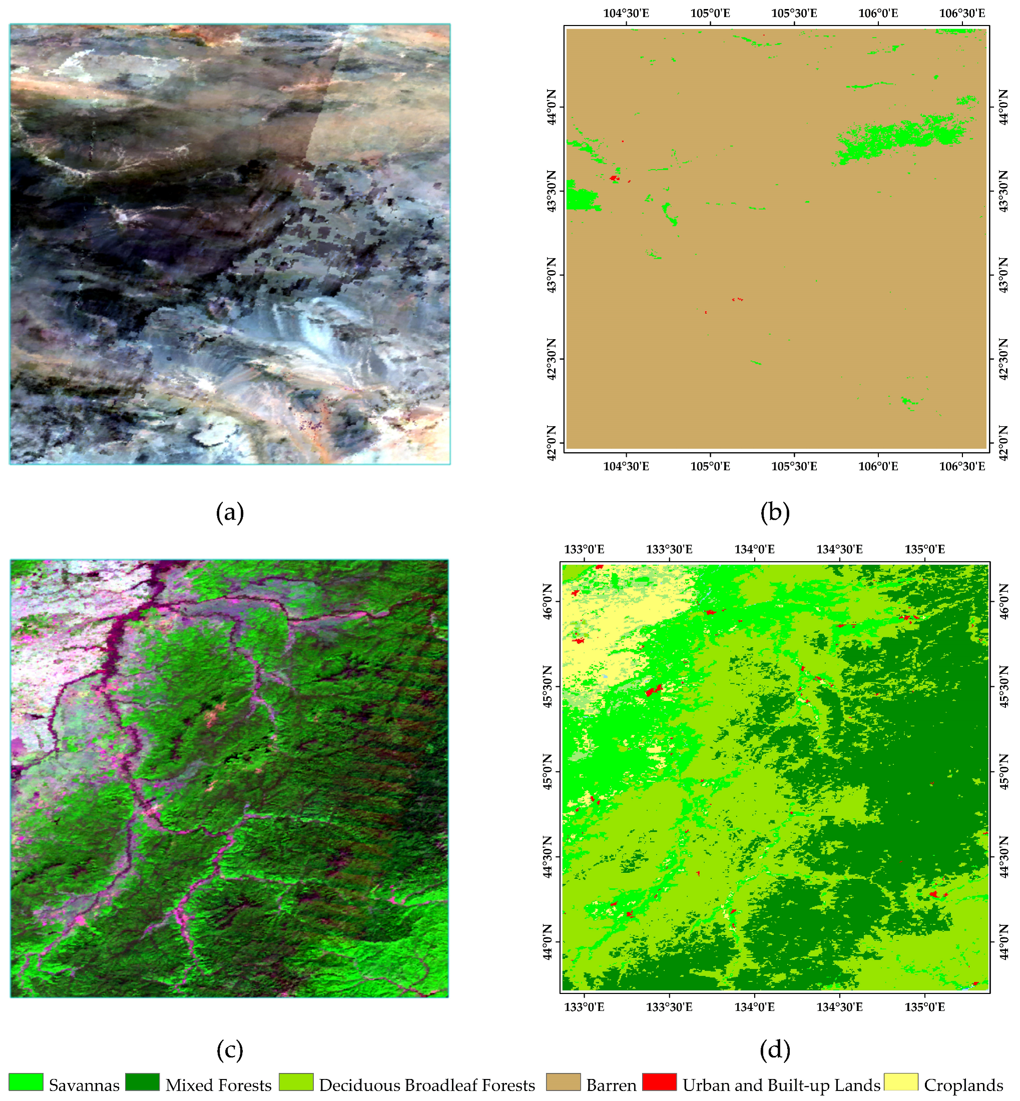
3.1. Experimental Data

This paper aims to evaluate the performance of an improved algorithm by utilizing the MOD09A1 product from the MODIS dataset, which is an eight-day composite of surface reflectance data. The basic characteristics of the MOD09A1 data are shown in

Table 1. Basic information of the MOD09A1 data product.

Data Product	Data Layer	Wavelength Range	Spatial Resolution	Temporal Resolution	Projected Coordinate System
MOD09A1	Surf_refl_b01	0.620–0.670 μm	500 m	8 days	Sinusoidal Projection
	Surf_refl_b02	0.841–0.876 μm
	Surf_refl_b03	0.459–0.479 μm
	Surf_refl_b04	0.545–0.565 μm
	Surf_refl_b05	1.230–1.250 μm
	Surf_refl_b06	1.628–1.652 μm
	Surf_refl_b07	2.105–2.155 μm

. To comprehensively verify the accuracy and applicability of the algorithm, we selected two scenes with different surface complexities for experimental analysis. Figure 3 shows two sets of experimental data, each with a size of 250 km × 250 km (500 × 500 pixels), representing scenes with single and complex surface types, respectively. Figure 3a shows data obtained on 26 June 2022 from a region in the central-western part of the Inner Mongolia Autonomous Region, with a latitude and longitude range of approximately 41°57′54″N to 44°27′54″N and 104°8′37″E to 106°38′37″E. Figure 3c shows data obtained on 14 September 2022 from the Russian Far East region, with a latitude and longitude range of approximately 43°42′54″N to 46°12′54″N and 132°52′18″E to 136°22′18″E. To ensure that the experimental areas accurately reflect the complexity of the surface coverage, Figure 3 shows the corresponding land cover classification based on the MCD12Q1 data and the IGBP classification standard for the areas shown in Figure 3b,d on the same dates.

It is important to note that data acquired from the same sensor at the same location may exhibit spectral differences across images captured at different times. These differences are caused by variations in observation conditions or land surface changes. Changes due to varying observation conditions typically have a smaller impact on image results and can be more easily corrected [48]. In general, to minimize the impact of these differences, the most temporally adjacent auxiliary images are selected. Therefore, we use images from both the immediate preceding and succeeding periods, as well as from the same periods in the preceding and succeeding years, to enhance the accuracy of the restoration process. The specific data used are shown in

Table 2. The acquisition date of the dataset and auxiliary data.

Dataset	Target Image Acquisition Date	Date of Auxiliary Data Acquisition
		8 Days Ago	8 Days After	Same Day the Year Before	Same Day the Year Later
Dataset1 (Single Surface)	2022.06.26	2022.06.18	2022.07.04	2021.06.26	2023.06.26
Dataset2 (Complex Surface)	2022.09.14	2022.09.06	2022.09.22	2021.09.14	2023.09.14

.

To reduce the impact of land surface changes, we introduced the Spectral Angle Mapper (SAM) in the algorithm to constrain multi-temporal data. Using the SAM values calculated by Equation (10), we analyzed the spectral similarity between each auxiliary temporal image and the target image to be restored, as shown in Figure 4. Figure 4a,c displays the SAM value distribution between the auxiliary temporal images and the target image in two scenarios, while Figure 4b,d presents the frequency distribution histograms of SAM values. It can be observed that the SAM values between all auxiliary images and the target image are almost all below 0.25. Further statistical analysis of the entire image reveals that over 96% of the pixels have SAM values less than 0.175 radians. This suggests that less than 4% of the area experiences land cover change, while over 96% of the area maintains high spectral consistency. The impact of land cover changes is minimal, thus making it reasonable to use the temporal data of the target image and its corresponding data from both the preceding and following periods, as well as the same periods from two years ago, for the restoration process.

3.2. Data Processing

3.2.1. Anomalous Pixel Identification

The MOD09A1 surface reflectance product inevitably suffers from imaging noise due to detector issues, as well as cloud, aerosol, and faulty detector elements, leading to anomalous pixel values for surface reflectance. The presence of these anomalous pixels compromises the authenticity and integrity of the data. The MOD09 user manual and the embedded quality control layer (surf_refl_qc_500m) and state layer (surf_refl_state_500m) describe the inversion quality of each pixel, as well as cloud and aerosol conditions. Based on this information, we identify and mark anomalous pixels, with specific rules for marking anomalous pixels, as shown in

Table 3. Rules for processing anomalous pixels.

Date Layer Name	Parameter Name	Bit Comb.	Pixel Processing Rules
Surf_refl_qc_500m	MODLAND QA bits	00	Retain
		Others	−28,672
Surf_refl_state_500m	Cloud state	00	Retain
		Others	−28,672
	Cloud shadow	0	Retain
		1	−28,672
	Aerosol quantity: level of uncertainty in aerosol correction	00	Retain
		01	Retain
		Others	−28,672
	Cirrus detected	00	Retain
		Others	−28,672
	Internal cloud algorithm flag	0	Retain
		1	−28,672
	Pixel is adjacent to cloud	0	Retain
		1	−28,672

. According to the valid data value range specified in the MOD09 user manual, all identified anomalous pixels are assigned the value −28,672, serving as a marker for pixels to be repaired subsequently.

3.2.2. Efficient Data Layer Extraction

The MOD09A1 data product not only includes the seven surface reflectance bands mentioned in Table 1, but also involves multi-dimensional data layers such as data quality indicators and observation geometry parameters (e.g., viewing angles, overpass times). Therefore, it is necessary to extract bands B1-B7 from the MOD09A1 dataset. Additionally, the MODIS data products are projected using sinusoidal projection, which results in significant image distortion. To facilitate analysis and application, these images are converted to the commonly used WGS84 geographic coordinate system projection. Based on this, 500 × 500 blocks are extracted from regions without anomalous pixels, representing high and low surface-type complexity scenarios (Figure 3), to conduct experiments simulating both artificial and real missing data. This experimental design aims to comprehensively validate and demonstrate the algorithm’s effectiveness and applicability in repairing different surface conditions, ensuring the feasibility and versatility of the algorithm.

3.3. Experimental Design

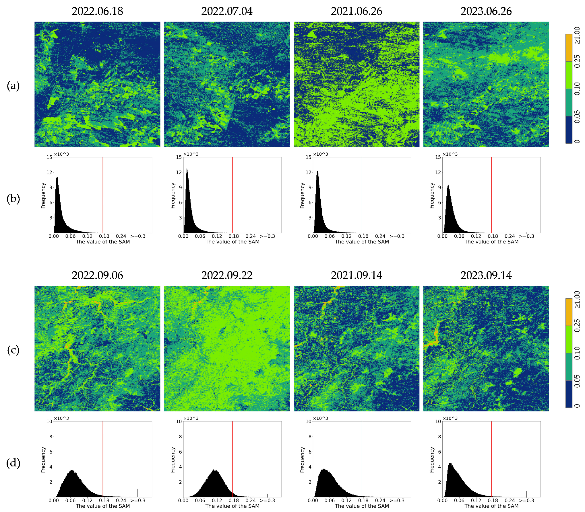
3.3.1. Simulated Experiment Design

In simulated experiments for remote sensing image inpainting, various types of masks can be used, including rectangular, linear, circular/elliptical, random pixel, and complex-shape masks. However, when the missing region is linear or stripe-shaped, more adjacent information can be obtained, making it easier to effectively repair the missing region, but this is not typical and oversimplifies real-world missing scenarios. Circular or elliptical masks and complex-shape masks can simulate some actual missing situations, but their irregular boundaries may introduce additional boundary effects. Random pixel masks can lead to overly scattered repair regions, making it difficult to evaluate the overall performance of the repair algorithm. In contrast, rectangular masks, with their clear boundaries and fewer adjacent pixels around the missing center pixels, create a more challenging repair environment, helping to assess the performance of repair algorithms under extreme conditions. This is useful for evaluating the capability of repair algorithms when there are fewer center missing pixels. Therefore, we chose rectangular masks for our simulation experiments to ensure that the experimental results better reflect the performance of the algorithm in practical applications.

During the simulated missing experiment phase of this study, we designed rectangular missing masks of different sizes to investigate the impact of the size of the missing region on image repair. Using rectangular masks ranging in size from 6 × 6 to 180 × 180, with each step increasing by 2, we simulated missing scenarios at different scales to observe and analyze the effect of increasing the area of the missing region on image repair.

3.3.2. Real Experiment Design

Real missing data are more complex and diverse than simulated missing data. To better reflect practical application scenarios, we selected real MOD09A1 data from 26 June 2022, acquired in North China, and used the missing data mask (as shown in Figure 5a). By overlaying the real missing data mask onto the target MODIS image for restoration (as shown in Figure 5b,c), we obtained five sets of real missing data with missing percentages of 2.44%, 4.66%, 5.22%, 11.51%, and 19.06%. This not only enhances the authenticity of the experiment but also ensures that the algorithm is tested in an environment that closely resembles the complexity of the natural environment and missing data. This approach validates the improved algorithm’s ability to achieve high-precision restoration in the face of dynamic and complex real-world conditions, thereby strengthening the algorithm’s reliability and effectiveness in practical applications.

3.3.3. Comparative Studies

To validate the effectiveness of the proposed algorithm, we selected three representative methods for comparison. These methods include two mathematical models, MNSPI [45] and WLR [48], and two deep learning models, STS-CNN [49] and PSTCR [50]. The deep learning models were used only in real data experiments. The MNSPI method restores missing regions by applying weighted spectral similarity. The WLR method reconstructs missing pixels by leveraging the relationships between missing and neighboring pixels through a regularization model. STS-CNN restores missing regions in remote sensing images by utilizing spatial–temporal–spectral information. PSTCR learns fundamental patterns and relationships within image patches through a stepwise spatio-temporal patch group approach. All methods were tested on the same dataset. For deep learning models, due to the limited availability of high-quality data caused by the small region missing problem, the models were primarily trained on small sample datasets.

3.3.4. Quantitative Evaluation

To evaluate the restoration performance of each model, we used three representative metrics: root mean square error (RMSE), peak signal-to-noise ratio (PSNR), and structural similarity index (SSIM). RMSE measures the error between the reconstructed and real images, PSNR assesses the accuracy of image restoration, and SSIM evaluates the structural and textural similarities between the reconstructed and real images. These metrics can be calculated as follows:

$$RMSE=\sqrt{{\displaystyle \frac{1}{n}}{\sum }_{i=1}^n{\left(L_i-\widehat{L_i}\right)}^2}$$

(15)

$$PSNR=10·{\log }_{10}\left({\displaystyle \frac{1}{RMSE}}\right)$$

(16)

$$SSIM={\displaystyle \frac{\left(2{{\mu }_L\mu }_{\widehat{L}}+{\theta }_1\right)\left(2{\sigma }_{L\widehat{L}}+{\theta }_2\right)}{\left({\mu }_L+{\mu }_{\widehat{L}}+{\theta }_1\right)\left({\sigma }_L+{\sigma }_{\widehat{L}}+{\theta }_2\right)}}$$

(17)

where $n$ is the number of pixels in the missing region to be restored; $L_i$ is the true image; and $\widehat{L_i}$ is the restored image; images $L$ and $\widehat{L}$ are evaluated via means ${\mu }_L$ and ${\mu }_{\widehat{L}}$, standard deviations ${\sigma }_L$ and ${\sigma }_{\widehat{L}}$, covariance σxy, and constants ${\theta }_1$ and ${\theta }_2$.

4. Experiment

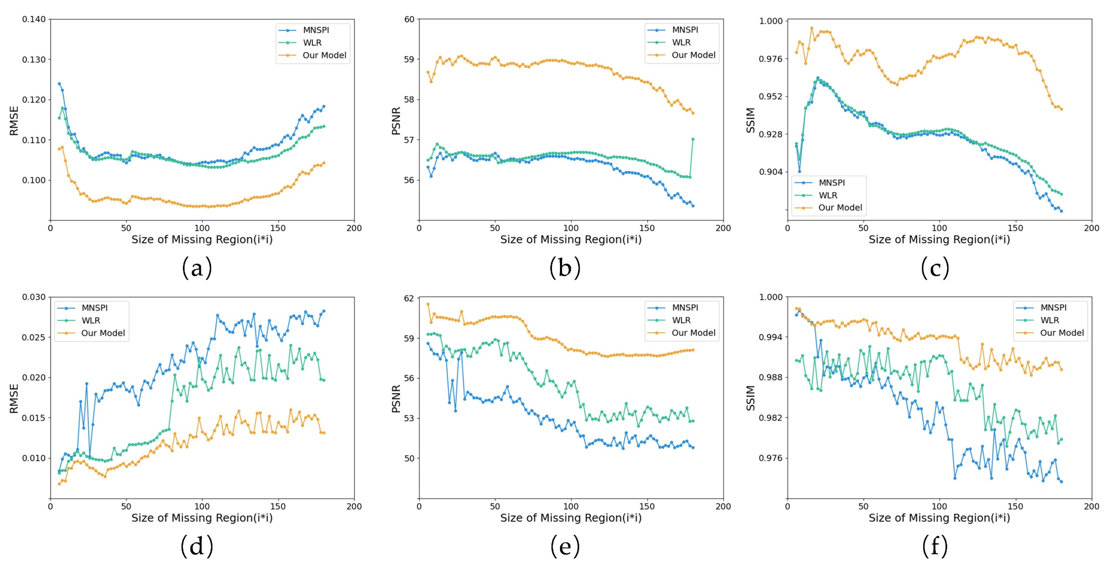
4.1. Simulated Experiment

In this study, we validated the proposed restoration algorithm through more than 90 simulated missing data experiments, assessing its performance under different land surface complexities and missing conditions. The experimental results are shown in Figure 6 and Figure 7, which, respectively, present the restoration results of the MNSPI algorithm, the WLR algorithm, and our algorithm. Additionally, Figure 8 provides a quantitative evaluation of the different missing levels. The results indicate that as the size of the missing area increases, all algorithms exhibit a decline in visual quality. The quantitative results in Figure 7 also show that although some fluctuations in accuracy may occur, the overall trend is a decrease in precision as the missing area expands. This suggests that the size of the missing region directly affects the performance of restoration algorithms, with larger missing areas posing greater challenges for accurate reconstruction.

Despite the impact of missing regions on algorithm performance, our method maintains superior restoration quality. As shown in Figure 6c and Figure 7c, when the missing region is 180 × 180 pixels, the MNSPI algorithm introduces noticeable restoration artifacts. In particular, the scene with a homogeneous surface in Figure 6c exhibits an outward diffusion pattern, while the complex surface scene in Figure 7c introduces some noise, affecting overall visual quality. The WLR algorithm results in severe structural feature loss, especially in homogeneous surface scenarios where the visual similarity between the restored and reference images is low. In contrast, our method consistently achieves better performance in both homogeneous and complex surface scenarios, demonstrating higher spectral continuity, clearer textures, and a visual appearance closer to the original image, thereby validating the effectiveness of our algorithm.

From a quantitative analysis perspective, our method also outperforms other methods, maintaining high accuracy even with larger missing regions. Notably, under a single surface type, the PSNR is approximately 2 dB higher and the SSIM is about 0.028 higher compared to other methods. Meanwhile, we observe that surface complexity influences restoration performance. As the missing region size increases, restoration results in complex surface scenarios are visually superior to those in homogeneous surface scenarios. The quantitative results in Figure 6 also show that in larger missing regions, the performance metrics for complex surface scenarios are consistently better than for homogeneous surfaces, aligning with findings from Chen [45]. This is because in complex surface scenarios, greater spectral variability and surface diversity provide more similar pixels for reference, enabling more accurate restoration, particularly in large missing areas.

Based on the evaluation of algorithm accuracy, we further explored the restoration capability of the proposed algorithm for missing regions of different sizes, focusing on situations where only similar pixels can be found. This allowed us to determine the optimal missing region size for the algorithm’s effective restoration. The statistics of unrestored pixels for missing regions of different sizes, shown in Figure 9c,f, indicate that in scenarios with relatively simple surface types, our algorithm can achieve the maximum restoration threshold for missing regions of 50 × 50 pixels. However, in scenarios with more complex surface types, this threshold is reduced to 44 × 44 pixels for the missing regions. Additionally, from the visual results in Figure 9b,e, when the missing region size is 180 × 180 pixels, we observed a significant number of unrestored pixels. Based on these results, we infer that for our algorithm, a missing region size of 44 × 44 pixels is the optimal size for effective image restoration. Therefore, we have updated the previous definition, where a region of 1024 pixels was considered a small missing area, and in this study, we define missing regions smaller than 1936 pixels as small missing regions.

4.2. Real Experiment

Compared to idealized simulated missing data, real-world data loss exhibits irregular and variable patterns. In this section, to further verify the effectiveness of the algorithm in restoring real missing data, five restoration experiments were conducted, with missing rates of 2.44%, 4.66%, 5.22%, 11.51%, and 19.06%. Similar to the simulated experiments, tests were performed on two scenarios with complex and simple land surface characteristics. The results are shown in Figure 10 and Figure 11, which present the restoration outcomes of the MNSPI algorithm, the WLR algorithm, the STS-CNN algorithm, the PSTCR algorithm, and our proposed algorithm. Additionally,

Table 4. Quantitative evaluation of the results of the real data experiment.

Method	Single Surface			Complex Surface
	RMSE	PSNR	SSIM	RMSE	PSNR	SSIM
MNSPI	0.229	49.735	0.989	0.130	56.748	0.994
	0.051	52.760	0.997	0.142	55.314	0.993
	0.132	54.463	0.996	0.128	56.961	0.994
	0.136	54.321	0.995	0.115	58.074	0.995
	0.169	52.413	0.995	0.133	56.571	0.994
WLR	0.121	55.273	0.996	0.118	58.590	0.997
	0.134	54.064	0.996	0.127	56.657	0.995
	0.132	54.589	0.987	0.111	57.908	0.995
	0.156	53.073	0.993	0.124	59.417	0.997
	0.186	51.524	0.990	0.126	57.791	0.996
STS-CNN	0.150	54.655	0.995	0.169	54.923	0.995
	0.196	53.585	0.995	0.252	53.787	0.993
	0.176	54.044	0.996	0.217	54.276	0.994
	0.189	51.970	0.994	0.283	53.696	0.992
	0.212	49.6580	0.989	0.349	52.537	0.988
PSTCR	0.054	52.536	0.997	0.029	56.335	0.996
	0.081	57.788	0.998	0.143	58.314	0.995
	0.129	54.347	0.996	0.162	52.112	0.994
	0.209	53.681	0.996	0.113	50.463	0.994
	0.282	50.964	0.993	0.234	57.039	0.995
Ours	0.103	56.989	0.996	0.091	59.347	0.997
	0.045	53.877	0.999	0.114	57.685	0.996
	0.119	54.728	0.997	0.107	58.026	0.996
	0.122	54.792	0.997	0.110	59.319	0.997
	0.143	53.638	0.996	0.111	57.948	0.996

Bold indicates the best performance, and underline indicates the second-best performance.

provides a quantitative evaluation of different missing levels, and Figure 12 illustrates scatter plots and R² values between real and reconstructed images, all validating the superiority of the improved algorithm.

From the visual restoration results, it can be observed that all algorithms show strong texture continuity and naturalness in images with smaller missing areas. However, when the missing areas are larger, the MNSPI algorithm causes the loss of some texture features, the WLR algorithm introduces noise, and there are visible restoration traces consistent with the results from the simulated experiments. In the experiment with 19.06% missing pixels, the restoration results of the STS-CNN and PSTCR algorithms are more blurred, and the color tone of the restored region differs from the complete region. Particularly in the complex surface feature scenario, the color tone differences between the restored images of the two deep learning models and the real images are more significant. On the other hand, our algorithm maintains better restoration quality visually, further validating the improvement in our algorithm. Comparing Figure 10 and Figure 11 with Table 4, it can be seen that when the missing region is large, the complex surface feature scenario yields better results, which is consistent with the simulated experiments and Chen [45] results. Based on the quantitative evaluation metrics, it can be observed that our method outperforms other methods, especially when the missing region covers 2.44% of the total area. In this case, our algorithm achieves a PSNR improvement of approximately 1 dB compared to the other algorithms. This further demonstrates the superiority of our algorithm in handling small missing regions.

To validate the applicability and accuracy of the restored data in quantitative applications, representative land cover types were selected, including grassland, cropland, forest, and a combined category of bare land and sparse vegetation. A comparative assessment of spectral fidelity was conducted based on the reconstruction results. As shown in Figure 13, the spectral reflectance curves reconstructed by the five algorithms are presented. The results indicate that the spectral curves generated by our improved algorithm are the closest to the actual ground values, successfully restoring the characteristics of surface reflectance. In particular, for grassland and forests, the spectral values reconstructed by our algorithm are nearly identical to the true values. The WLR method exhibits a noticeable underestimation of spectral values when processing bare land and sparse vegetation. The STS-CNN method performs well in the visible and infrared bands for grassland, but underperforms in the shortwave infrared band. The PSTCR method underestimates spectral values for bare land and sparse vegetation in the infrared band, while overestimating them in the visible band. Both deep learning models tend to overestimate spectral values for cropland and forests, with a particularly large difference of about 0.1 in the infrared reflectance of forests. Overall, our method maintains superior reconstruction performance across different land cover types, ensuring consistency between the restored spectral values and the true values.

4.3. Model Efficiency Analysis

Table 5. Comparison of training and prediction times for different algorithms.

Method	Model Training Time/h	Model Predicting Time/s	Adopted Equipment
MNSPI	/	33.59	CPU
WLR	/	26.04	CPU
STS-CNN	4.59	12.78	NVIDIA GeForce RTX 3090 GPU
PSTCR	6.22	15.27	NVIDIA GeForce RTX 3090 GPU
Ours	/	21.96	CPU

compares the time required for reconstruction and the computational resource demands for different methods applied to a 500 × 500 pixel image. From the perspective of processing time, deep learning models generally require less prediction time than mathematical models, and our method is second only to deep learning methods. Specifically, compared to the MNSPI algorithm, our method showed a significant 34.6% improvement in computational efficiency. Although the prediction phase of mathematical models is slightly longer than that of deep learning methods, their advantage lies in being directly applicable without the need for pre-training. While deep learning models have certain advantages in prediction speed, they require a large amount of high-quality data for training to ensure good generalization performance; otherwise, they may suffer from reduced generalization ability. Furthermore, for small region missing issues, deep learning models require high-performance GPUs and large sample datasets for training, while mathematical models can efficiently complete the restoration task with just an ordinary CPU. Therefore, when dealing with small region missing problems, mathematical models that require fewer computational resources and can provide stable and reliable restoration results are more suitable. Our method, with a relatively low prediction time, can achieve higher accuracy in reconstruction, demonstrating the superiority of the proposed algorithm.

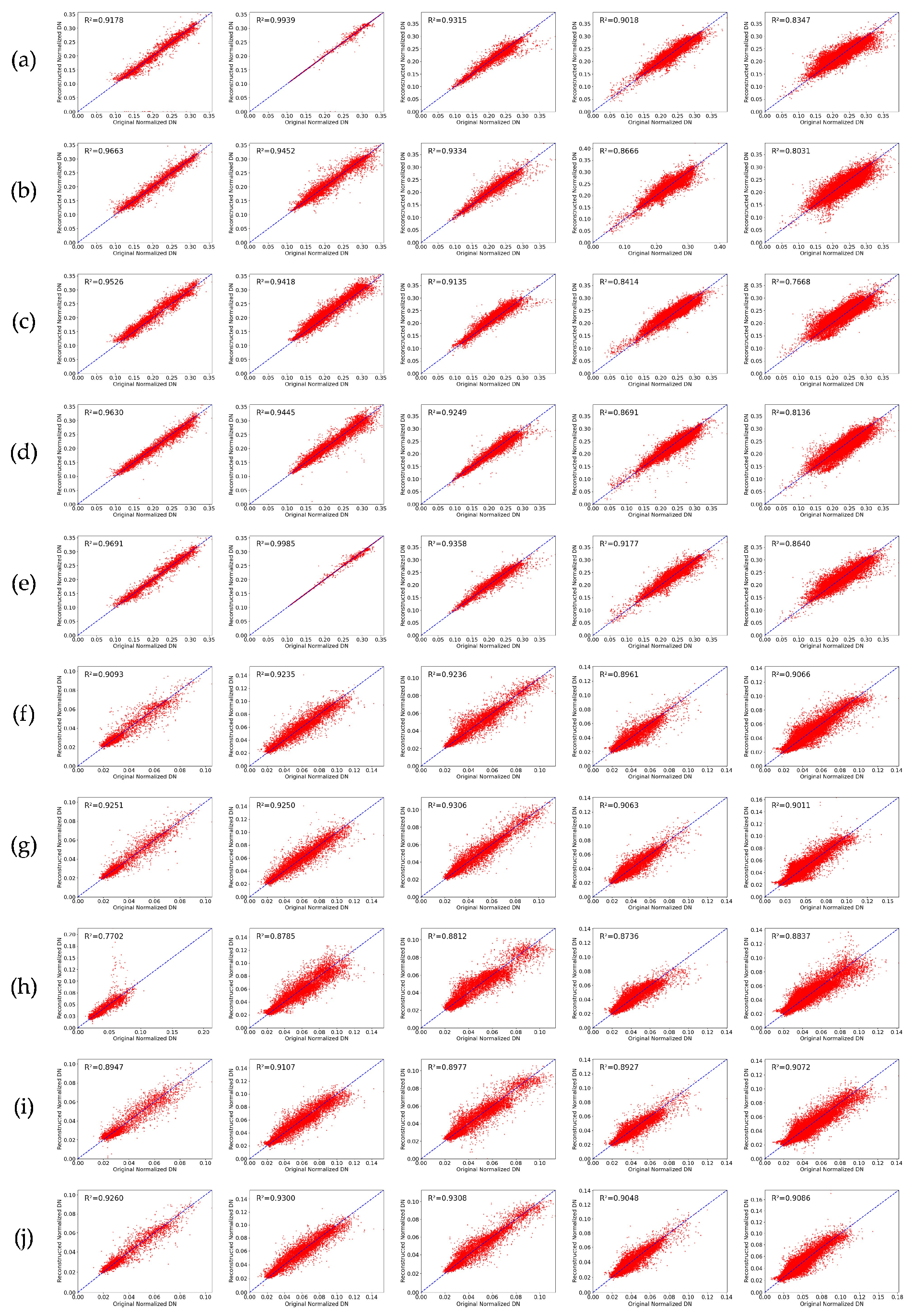
4.4. Globalization Applications

After comprehensive validation of the algorithm, the proposed small missing region data restoration method demonstrated high reliability. To verify the applicability of our method across different regions of the globe, we used MOD09A1 data acquired on 15 July 2023, along with the corresponding MOD09 quality control files. Following the small-region criteria defined in Section 4.1, we identified and restored small invalid pixels within connected regions where the number of pixels was fewer than 1936. Our experiment covers small-region missing data restoration for global real surface reflectance, and the comparison before and after restoration is shown in Figure 14. From the visualization results, it can be observed that small region missing issues are most prevalent in temperate continental climates, tropical savanna climates, and plateau mountainous climates. Zoomed-in regions show significant improvements in the small region missing issue, with the restoration effect being particularly notable in the temperate continental climate region represented by central China.

To analyze the extent of missing data, we used the MCD43A4 data product for validation. Given that the data still contain a substantial number of missing values, we selected three representative regions crucial for global climate regulation—the Amazon Basin, the Tibetan Plateau, and the Congo Basin—for further verification.

Table 6. Evaluation of reconstruction results for different regions.

	Tibetan Plateau	Amazon Rainforest	Congo Basin	Average
RMSE	0.0101	0.0188	0.0271	0.0187
MAE	0.0064	0.0132	0.0185	0.0127

presents the quantitative evaluation results for root mean square error (RMSE) and mean absolute error (MAE). Specifically, the Tibetan Plateau region exhibited the highest restoration accuracy, with the average accuracy being high across all three regions. The RMSE was 0.187, and the MAE was 0.127, further proving the accuracy of our method for restoring missing regions.

5. Conclusions

This study utilizes the characteristic that the spectral properties of ground objects do not change significantly within a short period of time. For small-region missing data, the study incorporates four temporal features and adaptively adjusts the weight of the temporal data based on the spectral similarity between pixels. A small-region missing data restoration algorithm suitable for low-resolution satellite data is proposed. The research was conducted in two scenarios with different surface complexities, and experiments were carried out on both simulated and real missing data. The results show that our method outperforms the comparison methods in all evaluation metrics. Additionally, in the simulated missing data experiments, we conducted tests where only similar pixels were considered and determined the optimal missing region size for the algorithm, which is defined as a region containing fewer than 1936 pixels in a connected area. In this study, such regions are referred to as small-region missing data. After comprehensive validation, the proposed small-region missing reconstruction algorithm was also applied to real global surface reflectance data reconstruction. The results indicate significant improvement in the small region missing issue, with average RMSE and MAE values of 0.0187 and 0.0127, respectively, in three typical regions, demonstrating the broad applicability of the algorithm worldwide.

At the same time, our algorithm does have certain limitations. First, like all methods using neighboring pixels, image restoration accuracy slightly decreases as the size of the missing region increases. Second, our experiments were conducted under conditions where land cover remained stable. Sudden events such as forest fires may lead to a decrease in restoration accuracy. Additionally, deep learning models have strong feature extraction capabilities. Considering the characteristics of missing data in MODIS, future work will explore deep learning models trained with small samples.

References

1. Liu, Y.; Zuo, X.; Tian, J.; Li, S.; Cai, K.; Zhang, W. Research on generic optical remote sensing products: A review of scientific exploration, technology research, and engineering application. IEEE J. Sel. Top. Appl. Earth Obs. Remote Sens. 2021, 14, 3937–3953. [Google Scholar] [CrossRef]
2. Wang, S.; Li, J.; Zhang, B.; Lee, Z.; Spyrakos, E.; Feng, L.; Liu, C.; Zhao, H.; Wu, Y.; Zhu, L.; et al. Changes of water clarity in large lakes and reservoirs across China observed from long-term MODIS. Remote Sens. Environ. 2020, 247, 111949. [Google Scholar] [CrossRef]
3. Zhao, X.; Hong, D.; Gao, L.; Zhang, B.; Chanussot, J. Transferable deep learning from time series of Landsat data for national land-cover mapping with noisy labels: A case study of China. Remote Sens. 2021, 13, 4194. [Google Scholar] [CrossRef]
4. Youssefi, F.; Zoej, M.J.V.; Hanafi-Bojd, A.A.; Dariane, A.B.; Khaki, M.; Safdarinezhad, A.; Ghaderpour, E. Temporal monitoring and predicting of the abundance of malaria vectors using time series analysis of remote sensing data through Google Earth Engine. Sensors 2022, 22, 1942. [Google Scholar] [CrossRef]
5. Justice, C.O.; Townshend, J.R.G.; Vermote, E.F.; Masuoka, E.; Wolfe, R.E.; Saleous, N.; Roy, D.P.; Morisette, J.T. An overview of MODIS Land data processing and product status. Remote Sens. Environ. 2002, 83, 3–15. [Google Scholar] [CrossRef]
6. Liu, Q.; Gao, X.B.; He, L.H. Haze removal for a single visible remote sensing image. Signal Process. 2017, 137, 33–43. [Google Scholar] [CrossRef]
7. Duan, C.; Pan, J.; Li, R. Thick cloud removal of remote sensing images using temporal smoothness and sparsity regularized tensor optimization. Remote Sens. 2020, 12, 3446. [Google Scholar] [CrossRef]
8. Xia, M.; Jia, K. Reconstructing missing information of remote sensing data contaminated by large and thick clouds bas ed on an improved multitemporal dictionary learning method. IEEE Trans. Geosci. Remote Sens. 2022, 60, 5605914. [Google Scholar] [CrossRef]
9. Yu, W.K.; Zhang, X.K.; Pun, M.O. Cloud removal in optical remote sensing imagery using multiscale distortion-aware networks. IEEE Geosci. Remote Sens. Lett. 2022, 19, 5512605. [Google Scholar] [CrossRef]
10. Yu, X.Y.; Pan, J.; Wang, M. A curvature-driven cloud removal method for remote sensing images. Geo-Spat. Inf. Sci. 2023, 26, 1–22. [Google Scholar] [CrossRef]
11. He, B.J.; Fu, X.C.; Zhao, Z.Q.; Chen, P.X.; Sharifi, A.; Li, H. Capability of LCZ scheme to differentiate urban thermal environments in five megacities of China: Implications for integrating LCZ system into heat-resilient planning and design. IEEE J. Sel. Top. Appl. Earth Obs. Remote Sens. 2024, 17, 18800–18817. [Google Scholar] [CrossRef]
12. Lin, T.Y.; Maire, M.; Belongie, S.; Hays, J.; Perona, P.; Ramanan, D.; Dollár, P. Microsoft COCO: Common Objects in Context. In Proceedings of the European Conference on Computer Vision (ECCV), Zurich, Switzerland, 6–12 September 2014; p. 5605914. [Google Scholar]
13. Zhou, J.; Jia, L.; Menenti, M.; Gorte, B. On the performance of remote sensing time-series reconstruction methods-A spatial comparison. Remote Sens. Environ. 2016, 187, 367–384. [Google Scholar] [CrossRef]
14. Alvaro, M.M.; Emma, I.V.; Marco, P.; Gustau, C.V.; Nathaniel, R.; Jordi, M.M.; Fernando, S.; Nicholas, C.; Steven, W. Multispectral high resolution sensor fusion for smoothing and gap-filling in the cloud. Remote Sens. Environ. 2020, 247, 11901. [Google Scholar]
15. Mikhail, S.; Eduard, K.; Nikolay, O.; Anna, V. A machine learning approach for remote sensing data gap-filling with open-source implementation: An example regarding land surface temperature, surface Albedo and NDVI. Remote Sens. 2020, 12, 3865. [Google Scholar] [CrossRef]
16. Yao, R.; Wang, L.C.; Huang, X.; Sun, L.; Chen, R.Q.; Wu, X.J.; Zhang, W.; Niu, Z.G. A robust method for filling the gaps in MODIS and VIRS land surface temperature data. IEEE Trans. Geosci. Remote Sens. 2021, 59, 10738–10752. [Google Scholar] [CrossRef]
17. Shi, B.B.; He, H.Q.; You, Q. A method of multi-scale total convolution network driven remote sensing image repair. J. Geomat. 2018, 43, 124–126. (In Chinese) [Google Scholar]
18. Tang, W.; He, F.Z. EAT: Multi-Exposure image fusion with adversarial learning and focal transformer. IEEE Trans. Multimedia. 2025, 27, 1–12. [Google Scholar] [CrossRef]
19. Tucker, C.J. Red and photographic infrared linear combinations for monitoring vegetation. Remote Sens. Environ. 1979, 8, 127–150. [Google Scholar] [CrossRef]
20. Field, C.B.; Behrenfeld, M.J.; Randerson, J.T.; Falkowski, P. Primary production of the biosphere: Integrating terrestrial and oceanic components. Science 1998, 281, 237–240. [Google Scholar] [CrossRef]
21. Myneni, R.B.; Hoffman, S.; Knyazikhin, Y.; Privette, J.L. Global products of vegetation leaf area and fraction absorbed PAR from year one of MODIS data. Remote Sens. Environ. 2002, 83, 214–231. [Google Scholar] [CrossRef]
22. Zhang, B.; Wu, Y.; Zhao, B.; Chanussot, J.; Hong, D.; Yao, J.; Gao, L. Progress and challenges in intelligent remote sensing satellite systems. IEEE J. Sel. Top. Appl. Earth Obs. Remote Sens. 2022, 15, 1814–1822. [Google Scholar] [CrossRef]
23. Wang, Y.; Zhang, B.; Zhang, W.; Hong, D.; Zhao, B.; Li, Z. Cloud Removal With SAR-Optical data fusion using a unified spatial-spectral residual network. IEEE Trans. Geosci. Remote Sens. 2024, 62, 1–20. [Google Scholar] [CrossRef]
24. Chu, D.; Shen, H.; Guan, X.; Chen, J.M.; Li, X.; Li, J.; Zhang, L. Long time-series NDVI reconstruction in cloud-prone regions via spatio-temporal tensor completion. Remote Sens. Environ. 2021, 264, 112632. [Google Scholar] [CrossRef]
25. Wang, Y.; Zhou, X.; Ao, Z.; Xiao, K.; Yan, C.; Xin, Q. Gap-Filling and Missing Information Recovery for Time Series of MODIS Data Using Deep Learning-Based Methods. Remote Sens. 2022, 14, 4692. [Google Scholar] [CrossRef]
26. Chen, H.; Chen, R.; Li, N.N. Attentive generative adversarial network for removing thin cloud from a single sensing image. IET Image Process. 2021, 15, 856–867. [Google Scholar] [CrossRef]
27. Chen, S.J.; Zhang, W.J.; Zhen, L. Cloud removal with SAR-Optical data fusion and graph-based feature aggregation network. Remote Sens. 2022, 14, 3374. [Google Scholar] [CrossRef]
28. Xu, M.; Deng, F.; Jia, S.; Jia, X.; Plaza, A.J. Attention mechanism-based generative adversarial networks for cloud removal in Landsat images. Remote Sens. Environ. 2022, 271, 112902. [Google Scholar] [CrossRef]
29. Shen, H.F.; Li, X.H.; Cheng, Q. Missing information reconstruction of remote sensing data: A technical review. IEEE Geosci. Remote Sens. Mag. 2015, 3, 61–85. [Google Scholar] [CrossRef]
30. Chen, S.J.; Zhang, W.J.; Zhang, B.; Kang, Q.; Xu, X. Research on method of surface reflectance reconstruction in the Tibetan Plateau based on MODIS data. Optics Precis. Eng. 2023, 31, 429–441. (In Chinese) [Google Scholar] [CrossRef]
31. Wang, Y.D.; Wu, W.; Zhang, Z.C.; Li, Z.M.; Zhang, F.; Xin, Q.C. A temporal attention-based multi-scale generative adversarial network to fill gaps in time series of MODIS data for land surface phenology extraction. Remote Sens. Environ. 2025, 318, 114546. [Google Scholar] [CrossRef]
32. Guillemot, C.; Le Meur, O. Image inpainting: Overview and recent advances. IEEE Signal Process. Mag. 2014, 31, 127–144. [Google Scholar] [CrossRef]
33. Hou, J.L.; Huang, C.L.; Wang, H.W. The cloud-removal method of MODIS fractional snow cover product based on kriging spatial interpolation. Remote Sens. Technol. Appl. 2014, 29, 1001–1007. (In Chinese) [Google Scholar]
34. Zhang, J.; Tan, Z.H.; Liu, M. Estimating land surface temperature under the cloud cover with spatial interpolation. Geogr. Geo-Inf. Sci. 2011, 27, 45–49+115. (In Chinese) [Google Scholar]
35. Tu, L.L.; Tan, Z.H.; Zhang, J. Estimation and error analysis of land surface temperature under the cloud based on spatial interpolation. Remote Sens. Inf. 2011, 4, 59–63+106. (In Chinese) [Google Scholar]
36. Tang, Z.; Wang, J.; Li, H.; Yan, L. Spatiotemporal changes of snow cover on the Tibetan Plateau based on cloud-removed moderate resolution imaging spectroradiometer fractional snow cover product from 2001 to 2011. J. Appl. Remote Sens. 2013, 7, 073582. [Google Scholar] [CrossRef]
37. Jing, Y.; Shen, H.; Li, X.; Guan, X. A two stage fusion framework to generate a spatiotemporally continuous MODIS NDSI product over the Tibetan Plateau. Remote Sens. 2019, 11, 2261. [Google Scholar] [CrossRef]
38. Scaramuzza, P.; Barsi, J. Landsat 7 scan line corrector-off gap-filled product development. In Proceedings of the Pecora, Sioux Falls, SD, USA, 23–27 October 2005; pp. 23–27. [Google Scholar]
39. Gerber, F.; de Jong, R.; Schaepman, M.E.; Schaepman-Strub, G.; Furrer, R. Predicting missing values in spatio-temporal remote sensing data. IEEE Trans. Geosci. Remote Sens. 2018, 56, 2841–2853. [Google Scholar] [CrossRef]
40. Zhang, X.; Zhou, J.; Liang, S.; Chai, L.; Wang, D.; Liu, J. Estimation of 1-km all-weather remotely sensed land surface temperature based on reconstructed spatial-seamless satellite passive microwave brightness temperature and thermal infrared Data. ISPRS J. Photogramm. Remote Sens. 2020, 167, 321–344. [Google Scholar] [CrossRef]
41. Shen, H.; Wu, J.; Cheng, Q.; Aihemaiti, M.; Zhang, C.; Li, Z. A spatiotemporal fusion-based cloud removal method for remote sensing images with land cover changes. IEEE J. Sel. Top. Appl. Earth Obs. Remote Sens. 2019, 12, 862–874. [Google Scholar] [CrossRef]
42. Li, X.; Wang, L.; Cheng, Q.; Wu, P.; Gan, W.; Fang, L. Cloud removal in remote sensing images using nonnegative matrix factorization and error correction. ISPRS J. Photogramm. Remote Sens. 2019, 148, 103–113. [Google Scholar] [CrossRef]
43. Li, M.; Zhu, X.; Li, N.; Pan, Y. Gap-Filling of a MODIS normalized difference snow index product based on the similar pixel selecting algorithm: A case study on the Qinghai-Tibetan Plateau. Remote Sens. 2020, 12, 1077. [Google Scholar] [CrossRef]
44. Xing, D.; Hou, J.; Huang, C.; Zhang, W. Spatiotemporal reconstruction of MODIS normalized difference snow index products using U-Net with partial convolutions. Remote Sens. 2022, 14, 1795. [Google Scholar] [CrossRef]
45. Zhu, X.; Gao, F.; Liu, D.; Chen, J. A modified neighborhood similar pixel interpolator approach for removing thick clouds in Landsat images. IEEE Geosci. Remote Sens. Lett. 2012, 9, 521–525. [Google Scholar] [CrossRef]
46. Chen, J.; Zhu, X.; Vogelmann, J.E.; Gao, F.; Jin, S. A simple and effective method for filling gaps in Landsat ETM+ SLC-Off images. Remote Sens. Environ. 2011, 115, 1053–1064. [Google Scholar] [CrossRef]
47. Qin, Y.; Guo, F.; Ren, Y.; Wang, X.; Gu, J.; Ma, J.; Zou, L.; Shen, X. Decomposition of mixed pixels in MODIS data using Bernstein basis functions. Appl. Remote Sens. 2019, 13, 046509. [Google Scholar] [CrossRef]
48. Zeng, C.; Shen, H.F.; Zhang, L.P. Recovering missing pixels for Landsat ETM+ SLC-off imagery using multi-temporal regression analysis and a regularization method. Remote Sens. Environ. 2013, 131, 182–194. [Google Scholar] [CrossRef]
49. Zhang, Q.; Yuan, Q.Q.; Zeng, C.; Li, X.H.; Wei, Y.C. Missing data reconstruction in remote sensing image with a unified spatial-temporal-spectral deep convolutional neural network. IEEE Trans. Geosci. Remote Sens. 2018, 56, 4274–4288. [Google Scholar] [CrossRef]
50. Zhang, Q.; Yuan, Q.Q.; Li, J.; Li, Z.W.; Shen, H.F.; Zhang, L.P. Thick cloud and cloud shadow removal in multitemporal imagery using progressively spatio-temporal patch group deep learning. ISPRS J. Photogramm. Remote Sens. 2020, 162, 148–160. [Google Scholar] [CrossRef]
Figure 1. Distribution of missing areas within global small regions, with red areas indicating missing data regions: (a,c,d) 256 × 256 pixel schematic diagrams for North America, Asia, and Oceania, respectively; (b) statistics on the size of missing areas in the Tibetan Plateau.
Remotesensing 17 01022 g001
Figure 2. Flow chart of improved MNSPI algorithm.
Remotesensing 17 01022 g002
Figure 3. Examples of experimental data with 500 × 500 pixels. (a,c) Single and Complex Land Cover Type Scenes; (b,d) Land Cover Classification for the Corresponding Scenes.
Remotesensing 17 01022 g003
Figure 4. Spectral similarity between auxiliary and target temporal phases. Here, (a,c) represent the spatial distribution of spectral similarity in two scenarios with different surface complexities, while (b,d) show the corresponding histograms of spectral similarity value distributions. The red line indicates whether the Spectral Angle Mapper (SAM) values are less than 0.175, representing high similarity.
Remotesensing 17 01022 g004
Figure 5. Real missing data at 500 × 500 pixels. (a) Missing mask (white represents colorless pixels, and black represents valid pixels); (b) single land cover type missing simulation; (c) complex land cover type missing simulation. In (b,c), the black areas denote the missing regions.
Remotesensing 17 01022 g005
Figure 6. Results of each method in the simulation experiment with a single surface type. The red boxes indicate the restoration areas and their magnified views. (a) Results for a missing area of 22 × 22 pixels; (b) results for a missing area of 50 × 50 pixels; (c) results for a missing area of 180 × 180 pixels.
Remotesensing 17 01022 g006
Figure 7. Results of each method in the simulation experiment with a complex surface type. The red boxes indicate the restoration areas and their magnified views. (a) Results for a missing area of 20 × 20 pixels; (b) results for a missing area of 44 × 44 pixels; (c) results for a missing area of 180 × 180 pixels.
Remotesensing 17 01022 g007
Figure 8. Quantitative evaluation of the results of the simulated data experiment. (a) RMSE results under a single surface type; (b) PSNR results under a single surface type; (c) SSIM results under a single surface type; (d) RMSE results under a complex surface type; (e) PSNR results under a complex surface type; (f) SSIM results under a complex surface type.
Remotesensing 17 01022 g008
Figure 9. Results of the improved MNSPI in two scenarios. (a,b) Results for a missing area of 50 × 50 and 180 × 180 pixels under a single surface type; (c) number of unrestored pixels in a scene of a single surface type; (d,e) results for a missing area of 44 × 44 and 180 × 180 pixels under a single surface type; (f) number of unrestored pixels in a scene of a complex surface type.
Remotesensing 17 01022 g009
Figure 10. Results of each method in the real data experiment for a single surface-type scene, with missing area proportions of 2.44%, 4.66%, 5.22%, 11.51%, and 19.06%. The red boxes indicate the restoration areas and their magnified views.
Remotesensing 17 01022 g010
Figure 11. Results of each method in the real data experiment for a complex surface-type scene, with missing area proportions of 2.44%, 4.66%, 5.22%, 11.51%, and 19.06%. The red boxes indicate the restoration areas and their magnified views.
Remotesensing 17 01022 g011
Figure 12. Scatter diagrams between the original and reconstructed pixels. (ae) Results of the MNSPI, WLR, STS-CNN, PSTCR, and our method under a single surface type; (fj) results of the MNSPI, WLR, STS-CNN, PSTCR, and our method under a complex surface type.
Remotesensing 17 01022 g012
Figure 13. Spectral curves of different feature types. (a) Grassland; (b) cropland; (c) forest land; (d) bare and sparsely vegetated land.
Remotesensing 17 01022 g013
Figure 14. Global restoration comparison image, with red areas indicating missing data regions. (a) Before restoration; (b) after restoration.
Remotesensing 17 01022 g014