Article

Multi-Temporal Relative Sea Level Rise Scenarios up to 2150 for the Venice Lagoon (Italy)

by
Marco Anzidei
1,2,*,
Cristiano Tolomei
1,
Daniele Trippanera
1,
Tommaso Alberti
1,
Alessandro Bosman
3,1,
Carlo Alberto Brunori
1,
Enrico Serpelloni
1,
Antonio Vecchio
1,4,5,
Antonio Falciano
6 and
Giuliana Deli
2
1
Istituto Nazionale di Geofisica e Vulcanologia, 00143 Roma, Italy
2
MARVE—Marine Archaeology Research Venice Equipe, Cannaregio 2999, Fondamenta Moro, 30121 Venice, Italy
3
Istituto di Geologia Ambientale e Geoingegneria, Consiglio Nazionale Delle Ricerche, CNR-IGAG, RU Sapienza DICEA, 00184 Rome, Italy
4
Radboud Radio Lab, Department of Astrophysics, IMAPP, Radboud University, 6500 GL Nijmegen, The Netherlands
5
Lesia Observatoire de Paris, Université PSL, CNRS, Sorbonne Université, Université de Paris, 92195 Meudon, France
6
Center of Integrated Geomorphology for the Mediterranean Area (CGIAM), 85100 Potenza, Italy
*
Author to whom correspondence should be addressed.
Remote Sens. 2025, 17(5), 820; https://doi.org/10.3390/rs17050820
Submission received: 23 December 2024 / Revised: 21 February 2025 / Accepted: 24 February 2025 / Published: 26 February 2025
(This article belongs to the Section Environmental Remote Sensing)

Abstract

:
The historical City of Venice, with its lagoon, has been severely exposed to repeated marine flooding since historical times due to the combined effects of sea level rise (SLR) and land subsidence (LS) by natural and anthropogenic causes. Although the sea level change in this area has been studied for several years, no detailed flooding scenarios have yet been realized to predict the effects of the expected SLR in the coming decades on the coasts and islands of the lagoon due to global warming. From the analysis of geodetic data and climatic projections for the Shared Socioeconomic Pathways (SSP1-2.6; SSP3-7.0 and SSP5-8.5) released in the Sixth Assessment Report (AR6) of the Intergovernmental Panel on Climate Change (IPCC), we estimated the rates of LS, the projected local relative sea level rise (RSLR), and the expected extent of flooded surfaces for 11 selected areas of the Venice Lagoon for the years 2050, 2100, and 2150 AD. Vertical Land Movements (VLM) were obtained from the integrated analysis of Global Navigation Satellite System (GNSS) and Interferometry Synthetic Aperture Radar (InSAR) data in the time spans of 1996–2023 and 2017–2023, respectively. The spatial distribution of VLM at 1–3 mm/yr, with maximum values up to 7 mm/yr, is driving the observed variable trend in the RSLR across the lagoon, as also shown by the analysis of the tide gauge data. This is leading to different expected flooding scenarios in the emerging sectors of the investigated area. Scenarios were projected on accurate high-resolution Digital Surface Models (DSMs) derived from LiDAR data. By 2150, over 112 km2 is at risk of flooding for the SSP1-2.6 low-emission scenario, with critical values of 139 km2 for the SSP5-8.5 high-emission scenario. In the case of extreme events of high water levels caused by the joint effects of astronomical tides, seiches, and atmospheric forcing, the RSLR in 2150 may temporarily increase up to 3.47 m above the reference level of the Punta della Salute tide gauge station. This results in up to 65% of land flooding. This extreme scenario poses the question of the future durability and effectiveness of the MoSE (Modulo Sperimentale Elettromeccanico), an artificial barrier that protects the lagoon from high tides, SLR, flooding, and storm surges up to 3 m, which could be submerged by the sea around 2100 AD as a consequence of global warming. Finally, the expected scenarios highlight the need for the local communities to improve the flood resiliency plans to mitigate the consequences of the expected RSLR by 2150 in the UNESCO site of Venice and the unique environmental area of its lagoon.

1. Introduction

The Venice Lagoon is located in the North Adriatic Sea, between the northeastern border of the Po Plain and the Grado Lagoon. The geological evolution of this area is driven by the dynamics of the foreland basin of the fold-and-thrust belts N-NE vergent of Northern Apennines and the S vergent Southern Alps [1]. It extends for about 550 km2 between the mainland and the Adriatic Sea, to which it is connected by the three inlets of Lido, Malamocco, and Chioggia (Figure 1). The lagoon, with its complex network of canals, islands, and salt marshes, is a unique fragile environment that has been settled since prehistoric times [2]. Since 1987, it has been recognized by UNESCO as a World Heritage Site, which is visited every year by about 30 million tourists. In addition, about 300,000 people live in the cities bordering the lagoon and the historical city of Venice, with a relevant impact on the environment [3]. The lagoon is thus exposed to multiple anthropogenic and environmental threats such as pollution, land subsidence, coastal erosion, and SLR [4,5,6]. The historical city of Venice and its lagoon, being placed close to the mean sea level (MSL), are particularly sensitive to SLR. In this area of the Mediterranean basin, the sea level (SL) is rising faster with respect to other coastal areas due to natural and anthropogenic land subsidence [4,6,7]. The first analyses carried out at the beginning of this century, by the Interferometric Synthetic Aperture Radar (InSAR) technique, found a downward vertical land movement (VLM) between 3 and 9 cm and the occurrence of a total relative sea level rise (RLSR) of 23 cm in the 19th century [8]. Further studies carried out in the last two decades highlighted the causes of the observed RSLR in more detail, such as the contribution of regional tectonics [9], the variability in VLM across the lagoon, and the regional atmospheric and oceanic processes [4]. However, predicting future effects on the coasts of the lagoon and the city of Venice remains a challenging task. This is due to the considered SLR projections and the reference emission scenario, the invariance assumptions of VLM rates or exposures, the accuracy of the geodetic data, the vertical resolution of the available Digital Elevation Models (DEMs) on which future sea levels can be projected, and finally, the method used to map the potential areas exposed to flooding [10]. The dominant cause of SLR in the Venice Lagoon has been anthropogenic local land subsidence due to groundwater withdrawal during the period of 1930–1970 [4] and the climate forcing due to the rise in global temperatures since 1800 AD, with the beginning of the industrial era, which is still continuing today [4]. The expected SLR is attributed to thermal expansion, the melting of glaciers and ice sheets, and changes in land water storage (www.ipcc.ch (accessed on 10 February 2025)). Since the instrumental era, sea level data from global tidal networks and radar altimetry observations over the oceans estimated a continuous SLR acceleration. The SL rate was 1.4 mm/yr in 1901–1990, then 3.6 mm/yr in 2005–2015, and about 4 mm/yr since 1993 [11,12]. According to the latest IPCC AR6 Report [11], the global mean SL is expected to rise as a function of the amount of CO2 emissions in the atmosphere. Indeed, in the low-emission scenario (SSP1-2.6), corresponding to net zero after 2050, the SL is expected to rise at a rate of 4–6 mm/yr, reaching up to 70 cm by 2100. In the worst-case scenario (SSP5-8.5), the rate is expected to be more than 10 mm/yr, corresponding to more than 120 cm by 2100 and up to about 5 m in 2300 [11]. After 2150, the SL will likely continue to rise for centuries due to the continuing heating of the oceans and the mass loss of the Greenland and Antarctic ice sheets. Since the SL changes along the coasts are caused by the sum of eustatic, glacial–hydro–isostatic, and tectonic factors [13], with gravitational patterns that depend on the melting of the polar ice caps and glaciers due to variations in the Antarctic and Greenland ice sheets [14], the SLR estimates will be larger in subsiding coasts, which will exacerbate coastal retreat and flooding at specific locations [15,16]. Therefore, to provide accurate local RSLR projections, which are essential to realize more reliable maps of flooding scenarios, it is crucial to include the contribution of VLM occurring along the coasts in the analysis. In this study, RSLR projections for the Venice lagoon were estimated through a multidisciplinary analysis by combining the current rates of change in SL and VLM, projected up to 2150, by summing the different contributions derived from (a) IPCC SLR projections [17] and (b) VLM from GNSS and InSAR instrumental data (that include the Glacial Isostatic Adjustment—GIA signal). In addition, we also analyzed SL trends collected at 25 tide gauge stations of the local network placed across the Venice Lagoon, which were compared with those located in the relatively tectonically stable areas of Trieste (North-East Adriatic Sea) and Genova (North Tyrrhenian Sea). The RSLR in the Venice Lagoon is already affecting the economy (infrastructures, tourism, etc.), environment (coastal ecosystems, biodiversity, inland migration, relocation of sediments), and society (decision-making practices, governance, policy domains, etc.). For this reason, it is important to disseminate results and to transfer scientific information to stakeholders and the coastal population to raise awareness of such phenomena. The assessment of VLM rates at mm accuracy was achieved by exploiting GNSS geodetic networks and space Earth Observation data. Land subsidence is a deformation phenomenon that is particularly relevant in the lowlands of coastal areas, often with high spatial heterogeneity [16,17,18]. GNSS measurements based on continuous monitoring stations provided data on the vertical velocity of the Earth’s surface at individual stations with sub-mm precisions. Conversely, InSAR captured both the local and the areal VLM occurring between the dates of acquisition of a time series of images [19,20,21] but with lower precisions. By combining the two geodetic datasets, the accuracy and spatial distribution of VLM estimates, RSLR projections, and related flooding scenarios were improved.
Here, we show and discuss new results on the expected RSLR projections and multi-temporal flooding scenarios for 2050, 2100, and 2150 AD for 11 specific areas of the Venice Lagoon (Figure 1). The maps of land flooding are shown on high-resolution topography extracted from LiDAR data. Our RSLR projections and flooding scenarios are suitable for assisting stakeholders, policy-makers and land planners in responding to short (2050 AD) and middle (2100–2150 AD) time horizons and preparing adaptation interventions and risk plans in response to RSLR.

Geodynamic Setting and Land Subsidence in the Venice Lagoon

The North Adriatic coast has been subjected to long-term subsidence since the Quaternary, occurring before the formation of the Venice Lagoon [2,22]. This area is affected by long-lasting horizontal and downward vertical crustal movements due to the dynamics of the Adria plate [9,23]. The latter drove the SLR, causing the continuous sinking of human settlements since the Roman age [2,6]. In addition, the natural consolidation of sediments also played a major role in the late Pleistocene and Holocene after the lagoon began to form, about 7000 years BP when the SL had been rising since the end of the last glacial maximum of 20,000 years ago [24,25,26]. The evaluation of the subsidence velocity, its spatial distribution, and the natural and anthropogenic origin in the Venice Lagoon has been a discussed issue in the last decades regarding the continuous sinking of Venice, particularly as a consequence of the ground fluid extraction and the subsequent measures to adopt for protecting the heritage site of Venice [6,8]. The mean natural subsidence rate of the lagoon has been estimated at 1.3 mm/yr, although this can vary between 0.4 mm/yr [24,25] and 1 mm/yr [9] from place to place.
On the other hand, anthropogenic land subsidence (LS) has had large impacts on the cities of Venice and Marghera. In particular, this was driven by the intensive depletion of artesian aquifers that exploited water from buried consolidated Quaternary formations. Groundwater withdrawals and subsequent land sinking started with the onset of the industrial installations after 1930 and reached their maximum between 1950 and 1970. During this period, the industrial zone of Marghera, the southern lagoon, the city of Venice, and the northeastern lagoon, experienced sharp and high rates of LS. In particular, between 1968 and 1969, values greater than 17 mm in Marghera and 14 mm in Venice led to a total subsidence of 14 cm in the industrial area and 10 cm in Venice in the period of 1952–1969 [4]. As a consequence of the effects on the city of Venice and the surrounding zones, drastic measures have been taken to cut fluid extractions since 1970. The adopted measures led to a rapid reduction in LS, which finally ended in 1973 [27].
To monitor the evolution of the VLM trend, a leveling network consisting of about 400 benchmarks was established in Venice and the surrounding areas and repeatedly surveyed over time [28]. In the past, the evaluation of subsidence rates was estimated through different techniques, including stratigraphy [29], 14C dating of sediments [26], tide gauge data [7], archaeological and historical data [2,30], and the combination of space-based geodetic data of Synthetic Aperture Radar (SAR) Interferometry and GNSS networks [31]. These studies tentatively clarified the origin of land subsidence due to the combination of long-term components controlled by the tectonic subduction associated with the Apennines (of about 106 yr) and short-term components controlled by glaciation cycles due to climatic changes (103–104 yr) [25,29]. The variability of LS across the lagoon needs to be further evaluated thanks to the availability of sufficiently long time series of new geodetic data. This is a relevant issue, especially when linked with global warming and the consequent joint impact of SLR and land subsidence, to estimate the flooding scenarios in the lagoon for the next decades.

2. Materials and Methods

To estimate the expected effects of RSLR for different zones of the Venice Lagoon by 2150 AD and realize multi-temporal maps of the expected flooding scenarios, we used a multidisciplinary approach that included geodetic, sea level, and climatic data, namely, (i) geodetic data from the GNSS networks distributed in the Venice Lagoon and surrounding areas to measure the ground velocity at specific locations in the period of 1996–2023 (Table 1); (ii) remote sensing data from SAR satellites to estimate the current rates of spatial VLM in the period between June 2017 and October 2023; (iii) time series of sea-level data collected in the period of 1996–2023 at the tide gauge network managed by ISPRA and the Tide Center of the Municipality of Venice; (iv) LiDAR data obtained from CO.RI.LA (Consortium for the coordination of research relating to the Venice Lagoon system, https://www.corila.it/ (accessed on 20 February 2025)) and the Italian Ministry of the Environment to extract high-resolution DSMs and project the potential extension of flooding scenarios for different SSPs; and, finally, (v) the revised IPCC AR6 sea level projection to 2150 for the SSP1-2.6, SSP3-7.0, and SSP5-8.5 climatic scenarios for the Mediterranean basin.

2.1. Geodetic Analysis

VLM from GNSS Data

The geodetic VLM rates were obtained by integrating InSAR velocities and GNSS three-dimensional velocities. As regards the GNSS data, we used a subset of the Euro-Mediterranean velocity solution, as reported in [30], which included continuous GNSS networks operating in the Venice Lagoon (e.g., Italian Space Agency—ASI, Geodetic Data Archive Facility—GeoDAF, EUREF Permanent Network—EPN, Friuli Regional Deformation Network—OGS-FredNet, and GNSS National Integrated Network—INGV-RING).
Data retrieved from these networks are routinely downloaded, archived, and processed by the INGV data analysis center together with other regional and private networks (e.g., the EPOS GNSS data portal at https://gnssproducts.epos.ubi.pt/ (accessed on 20 February 2025); the Hexagon SmartNet at https://hxgnsmartnet.com/ (accessed on accessed on 20 February 2025)), consisting of about 360 stations; and the Topcon NetGeo at https://shop.netgeo.it/ (accessed on 20 February 2025), consisting of about ~230 sites in Italy (for a complete list, see [32]). In the analysis, we considered all the data available from 1995 to 2023. The raw GNSS observations were analyzed using GAMIT/GLOBK software (v. 10.71, 9 March 2020), following the three-step procedure described in [32], to which we refer for any additional detail on the GNSS data processing. The daily GAMIT solutions were combined using GLOBK software, which adopts a Kalman filter estimation algorithm to simultaneously realize a global reference frame by applying generalized constraints. Specifically, the reference frame was obtained by minimizing the velocities of a set of core stations (https://network.igs.org/ (accessed on 20 February 2025)) while estimating a seven-parameter transformation of the GNSS realization of the ITRF2014 frame (i.e., the IGb14 reference frame). The position time series were later analyzed to estimate the 3 components (east, north, and vertical), linear velocities, and uncertainties, accounting for offsets due to changes in the station’s seismic equipment and non-linear motions due to eventual post-seismic deformations, assuming a white–flicker noise model (see the procedure described in [32]). Only stations with a minimum time span of 4.5 years were included in the analysis. This was performed to avoid biases due to unreliable estimated seasonal signals and underestimated velocity uncertainties due to absorbed correlated noise content in estimated trends of short time series. The estimated vertical velocities and uncertainties for the stations used in the integration step with InSAR are shown in Table 1.

2.2. InSAR Analysis

Displacement time series of geodetic data from Multi-Temporal Interferometric Synthetic Aperture Radar (MT-InSAR) allowed us to study the temporal and spatial behavior of the ground motion of the investigated area. During the last two decades, the MT-InSAR approach was developed to overcome the issues relative to the standard InSAR methodology [33,34,35], taking advantage of using a large data stack of SAR images to obtain displacement time series and the associated mean ground velocities. The current algorithms fall into two broad categories, namely, the Permanent Scatterer® (PS) (technique manufactured by Telerilevamento Europa T.R.E., Milan, Italy) [36,37] and the Small Baseline (SB) [38] approaches, although more recently, algorithms exploiting the basic principles of both methodologies have also been proposed [39,40]. The PS methods aim to identify coherent radar targets exhibiting a high signal phase and amplitude stability over the whole temporal span of the observations [36], i.e., a dominant single scatter in the SAR resolution cell. These targets are only slightly affected by temporal and geometrical decorrelation. These PSs can be natural or man-made objects, such as buildings, rocks, or other structures that remain stable and highly reflective over time. By analyzing the phase differences in SAR images acquired at different times (i.e., image by image), the technique can estimate ground movements with millimeter accuracy [41]. In contrast, in the original SB approach [38], interferometric pairs are chosen to minimize temporal and geometric decorrelation. This allows us to retrieve deformation time series for the so-called distributed scatterers (i.e., neighboring radar resolution cells), which are not dominated by a single scatterer and share the same backscattering properties. In the best case, both the PS and SB multi-temporal InSAR approaches can reach accuracies of ±1.5 mm/yr [41,42]. In addition, MT-InSAR offers a wide area of coverage, making it a cost-effective solution for large-scale deformation monitoring. Integrating MT-InSAR data with other geospatial information systems enhances decision-making processes in risk management and urban planning. In our analysis, we used the Enhanced PS (EPS) [37], a technique that differs from the PS as it takes into account not only standard PSs but also distributed scatterers (DSs), resulting in a wider spatial coverage. Unlike traditional PS methods that rely solely on PSs, which are stable, radar-reflective points, EPS also leverages DSs, which are more numerous scatterers providing additional measurement points. This PS/DS combination increases the density and reliability of point data, particularly in areas where PSs alone are insufficient, such as non-urban environments or regions with diverse terrains. Such a combination allows for a more comprehensive and detailed deformation map and offers a clearer picture of the underlying geophysical processes.

2.3. EPS Analysis

We collected 187 images along the descending orbit (track 95) acquired by the Sentinel-1 (S1) Copernicus constellation (C-Band), which is operated by the European Space Agency in the TOPSAR acquisition mode. The temporal interval spanned between 22 June 2017 and 25 October 2023, while the ALOS-World 30 m Digital Elevation Model was used to remove the topographic contribution. A double-filtering operation (high and low pass, time and space, respectively) was applied to estimate and remove the atmospheric noise. Finally, a geocoding step was performed to obtain the displacement time series and the ground velocity map.
Finally, with regard to the area under investigation, we assumed that the expected ground motion is purely vertical; hence, neglecting the horizontal movement does not involve a significant error. The latter implies that retrieving the Up/Down velocity map from the descending SAR Line of Sight (LoS) is sufficient to divide the retrieved measurements by the cosine of the incidence angle (i.e., 38.87°). In the post-processing analysis to validate the InSAR product, we compared the results with the InSAR outcomes from the descending data (not calibrated ones) obtained in the European Ground Motion Service (https://egms.land.copernicus.eu/ (accessed on 20 February 2025)). We observed a very good agreement between our results and the other data sources, both in terms of spatial patterns and temporal trends. Subsequently, we referred the InSAR descending data to the VEN1 GNSS station (Table 1) chosen as a reference to calibrate the InSAR ground velocities. We selected this specific GNSS station because it is located in the inner island of Venice, where the InSAR results show a full spatial coverage and the time series is stable and longer than 4.5 years. Then, the vertical GNSS velocities were compared with the SAR velocities, where data from both techniques overlapped (for the InSAR products, we selected data included in a buffer of at least 100 m radius around each GNSS station). The result of the comparison is reported in Figure 2, showing a good agreement with an RMSE of 0.41 mm/yr and a mean value for the GNSS-InSAR difference of 0.35 mm/yr.
The comparison of Vup between InSAR and each GNSS station (Figure 2) is encompassed within the −1.5 ± 1.5 mm/yr range. The latter is largely within the respective accuracies of the two techniques, thus ensuring the reliability of the retrieved results. The final ground velocity map for the Up component, starting from the S1 descending map, after the aforementioned calibration, is shown in Figure 3. The mean velocity field was obtained by applying the Enhanced PS approach in the SARscape® software v.5.7 included in the ENVI (NV5) package. Then, we focused our analyses on the areas highlighted in Figure 1. This includes the island of Venice, the three inlets of the MoSE system with the open sea, the Marco Polo airport, the Island of St. Erasmo, and the three sandy coasts of Lido Cavallino, Lido Venezia, and Lido Malamocco, which face the North Adriatic Sea, and the low elevated areas of Chioggia and Marghera, with their economic infrastructures. The above areas are affected by variable rates of land subsidence, as reported in Table 2.

2.4. Tide Gauge Analysis

In the Venice Lagoon, 25 gauge stations are operational, including the historical one located at the Punta della Salute, which has recorded sea level data since 1872 (see Figure S2 and Table S1 in the Supplementary Materials) [43]. They belong to different agencies, namely, the Italian Istituto Superiore per la Ricerca Ambientale (ISPRA), the Municipality of Venice, and the National Research Council (CNR). In particular, a set of stations is managed by the Tide Center of the Municipality of Venice (https://www.comune.venezia.it/it/content/centro-previsioni-e-segnalazioni-maree (accessed on 20 February 2025)) and ISPRA (www.mareografico.it (accessed on 20 February 2025)). The analysis of the time series of monthly MSL data collected in the last 38 years shows a mean trend of 5.1 ± 0.7 mm/yr (Figure 4). The difference in the estimated rates, which range between 2.8 ± 1.3 mm/yr at Malamocco Porto and 6.9 ± 0.7 mm/yr at San Nicolò, is due to the relative sea level variability, which shows a minimum flexure coincident with the beginning of the recordings of the local network and the spatial variability in VLM across the lagoon (for details, see Figure S2 and Table S1 in the Supplementary Materials).

2.5. High-Resolution Digital Surface Models (DSMs)

Depending on the coverage dataset, we used the land topography obtained by airborne LiDAR data collected by the CO.RI.LA in 2018 (the Consortium for the coordination of research relating to the Venice lagoon system, https://www.corila.it/ (accessed on 20 February 2025)) and by the Italian Ministry of the Environment in 2008. The final Digital Surface Model (DSM) for each area was generated with a 1 m cell size. The vertical ellipsoidal altitudes were reported to the ItalGeo 2005 Geoid Model released by the Italian Istituto Geografico Militare, with elevation Datum referred to the MSL at the tide gauge station of Genova, in 1942 AD [44]. In order to have a realistic estimate of the flooded area, the amount of the total VLM for each area (and, therefore, the overall changes in the local topographic altitudes) at 2050, 2100, and 2150 were calculated considering the epochs when the LiDAR data were acquired (years 2008 and 2018).

3. Results

In the following section, we show the results of the combined data analysis, namely, the projected sea levels up to 2150 for different climatic scenarios of the IPCC AR6 and the multi-temporal maps of flooding for 2050, 2100, and 2150 AD for the investigated areas.

3.1. Relative Sea Level Rise Projections

To project the expected sea levels for the Venice Lagoon, the latest climatic projections based on the IPCC AR6 (available at https://zenodo.org/record/6382554 (accessed on 20 February 2025)), were adopted. The estimates consist of median sea-level values and standard errors on a worldwide grid obtained by summing up the contributions of geophysical sources that are driving the long-term sea level changes. As for the IPCC AR6, projections are provided for SSPs 2.6, 7.0, and 8.5. In the SSP1-2.6 scenario, the emissions of greenhouse gases peak around 2020, while in SSP5-8.5, they continue to grow throughout the century [17]. In this study, we used the regional projection including medium uncertainty processes (file ar6-regional_novlm-confidence.zip). The projected SLR was estimated by combining the SLR rate at the grid point closest to coordinates 45 N, 13 E, as provided by the IPCC projections, with the rate of VLM inferred from the geodetic analysis reported in Chapter 4. In detail, the measured rate of VLM, which includes GIA and tectonic components of both natural and anthropogenic origin, replaces the modeled GIA contribution used in the original IPCC AR6 projections. The total uncertainty depends on both the IPCC projection and the VLM uncertainties. It was calculated as the square root of the sum of the squared uncertainties from the AR6 IPCC projections (as the distribution spread estimated from the 17th and 83rd percentiles) and the squared error from InSAR data. Errors coming from the InSAR data are included in the overall uncertainty estimation (Supplementary Materials S5).
Considering a constant rate of VLM until 2150 AD, the total amount of the VLM component for each area is strictly related to the time spanning from the reference year (or benchmarking year) to the projection year. Adopting the epoch 2023 AD as the benchmark year from the IPCC report AR6, the durations of time spans for the projections are 127, 77, and 27 years for 2150, 2100, and 2050, respectively. By using the same time span for the total VLM calculation, the RSLR at 2150 for an SSP 8.5 scenario may increase from 11 to 37 cm compared to the IPCC estimates depending on the considered area (Table 3 and Supplementary Materials S5).

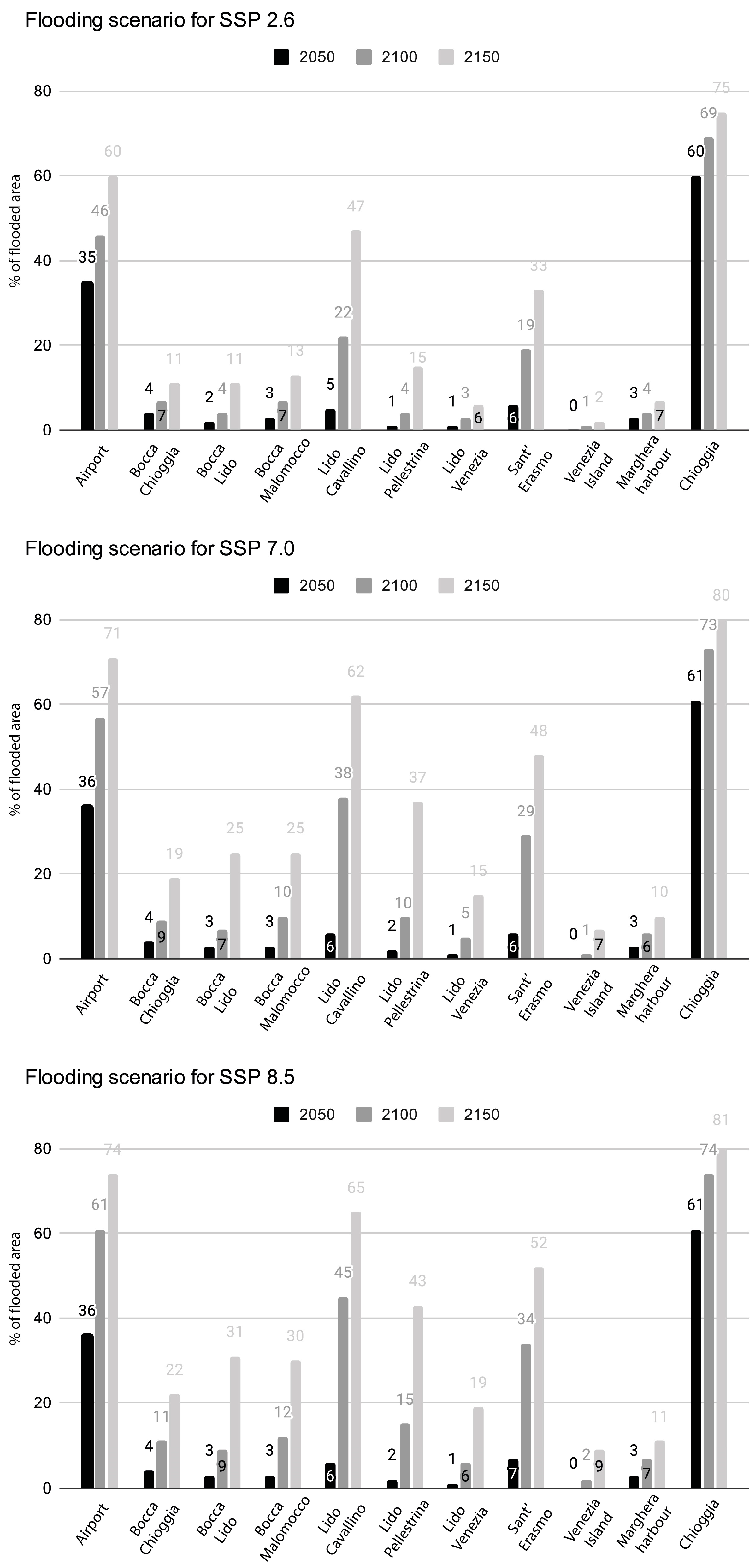
3.2. Flooding Scenarios for 2050, 2100, and 2150

The combined analysis of VLM, RSLR projections, and high-resolution topography allowed for the assessment of the multi-temporal flooding scenarios for 2050, 2100, and 2150 across the Venice Lagoon. To refine the characterization of the areas prone to RSLR and the accuracy of the expected flooding assessment, the investigated area was divided into different Areas Of Interest (AOI), for which the current VLM rates were evaluated individually. Moreover, due to the different time spans of the LiDAR dataset acquisition (from 2008 to 2018), the total amount of VLM used to create the flooding maps for each area was calculated based on the data acquisition of LiDAR topography. In this way, the local RSLR projections and flooding scenarios are provided at high spatial resolution, thus becoming more representative for specific areas. Finally, the multi-temporal flooding scenarios were mapped for each AOI. The results consist of a set of flooding maps showing the potential scenarios of marine inland extension for 2050, 2100, and 2150 for the targeted areas. We clarify that the spatial extent of the potentially flooded areas was estimated through a standard passive “bathtub” approach. A zero-connectivity rule for each area that falls below a defined water level and is not necessarily hydraulically connected to the sea was used and considered flooded [45]. In addition, the flooding scenarios do not take into account any adaptation or protection system, such as the MoSE. Despite the limitations of the method, this approach can be acceptable to define the flooding hazard for a coastal region, especially in the absence of detailed hydraulic features [46,47,48,49,50]. In Figure 3, Figure 5, Figure 6, Figure 7, Figure 8 and Figure 9 and the Supplementary Materials (Figures S1.1–S1.11 and S4.1–S4.11), the maps of land subsidence, the expected extension of flooding areas, and the potential inundation scenarios for each study area, based on the future RSLR projections for different SSPs reported in Table 3, are shown.
We clarify that the inundated areas shown on our maps were estimated based on the water levels above the DSM previously obtained from the analysis of LiDAR data. The latter is referred to as the Geoid model Italgeo2005 [44]. Hence, the adopted elevations in this paper are 23 cm higher with respect to the historical benchmark of the Punta della Salute tide gauge station (ZMPS altimetric reference level established in 1897 adopted by the Municipality of Venice to measure the water levels in the Lagoon (for further details, see https://www.comune.venezia.it/it/content/le-percentuali-allagamento (accessed on 20 February 2025)). This means that the surfaces exposed to flooding shown in our maps differ from those of the Municipality of Venice for the respective water levels within the city. So, in the case of the Island of Venice, when an RSLR of 130 cm is considered with respect to the Italgeo2005 Geoid, it corresponds to an RSLR of 153 cm with respect to the ZMPS of the Punta della Salute tide gauge. This implies that the corresponding flooded surface would differ from about 9% to about 73%, respectively.
Concerning the flooding scenarios, we also considered the amplitude of water levels during past extreme events. For example, we considered the 1966 AD event, when the SL reached the highest known value ever recorded of +1.94 m during a storm surge that occurred with the combined contribution of atmospheric forcing and tidal cycle (Figure 5, Figure 6, Figure 7, Figure 8 and Figure 9). However, recent analyses of the second historical high water maximum in 2019 suggested that the SL may have reached 2.10 m [48]. Therefore, to estimate the extreme scenario for 2150, in this study, we considered the Maximum High Water Level (MHWL) that occurred during the 1966 event as a reference, which was added to the expected RSLR at 2150 for the SSP 8.5 scenario. The inundated areas shown on the maps correspond to the estimated water levels that propagate inland over the DSM. The variability in LS across the lagoon drives the different RLSR projections and the consequent extension of inundation scenarios for the different areas of the lagoon. The highest rates of LS, which reach up to 7 mm/yr, mainly occur in the proximity of the coastlines and man-made structures, such as wharves, piers, and disembarkation areas (see Figure 5, Figure 6, Figure 7, Figure 8, Figure 9 and Figure S4.1–S4.11 in the Supplementary Materials). Subsidence and coastal retreat phenomena are also retrieved along the coastal sector near the MoSE dams, where breakwaters are located (especially for the MoSE inlet of Chioggia), at rates of ~3 mm/yr. It is worth noting that some man-made structures, such as the concrete branches of the inlet to the Venice Lagoon at Chioggia, show different lowering velocity rates along their length. This behavior could imply eventual differential structural settlement over time, which may occur in concrete maritime constructions exposed to SLR [51].

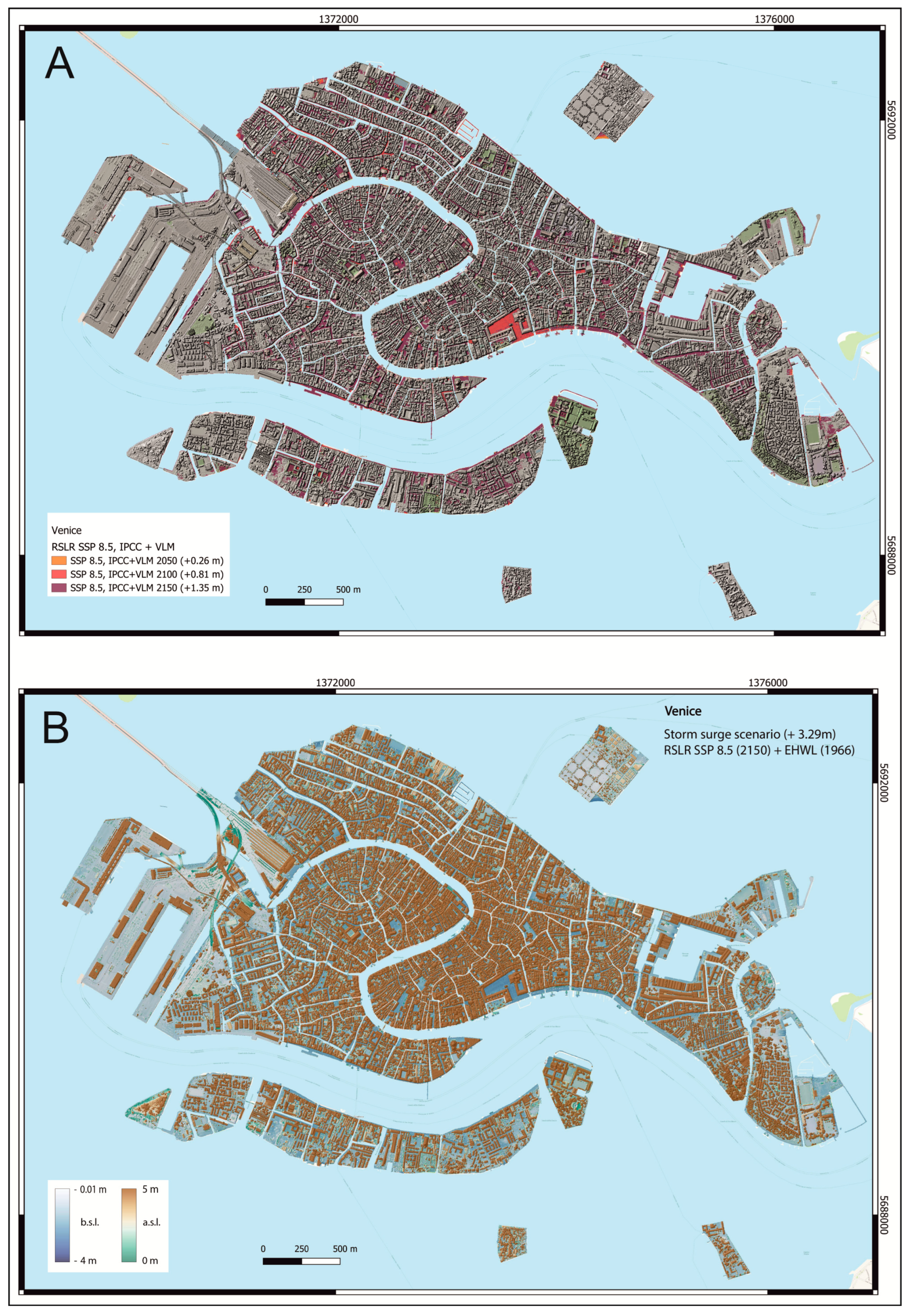
3.2.1. Area 1—The City of Venice

The city of Venice is located on the largest island of the lagoon (Figure 1). The VLM of this area shows smaller values with respect to the nearby areas due to better vertical stability of the ground that reflects the regional tectonics at about −1.4 mm/yr (Table 1) [2,32]. This implies that the RSLR projections and flooded areas for this location show lower values. Considering the SSP5-8.5 scenario, the expected RSLR for 2150 is up to 1.34 m (or 1.35 m considering 2018 as a benchmarking year), with a potential flooding surface of 0.63 km2. This value corresponds to about 9% of the analyzed DSM surface. However, the surface of the DSM we considered in Venice is 6.9 km2, of which 2.7 km2 is occupied by buildings. Therefore, the total surface exposed to flooding corresponds to 23% of the surface not occupied by buildings alone. In the case of extreme events, instead, the flooding surface corresponds to more than 36% (if we consider the total DSM) or 59% (when we consider only the area not covered by buildings) (see Table 2 and Table 4; Figure 5 and Figures S1.1, S3 and S4.1; and Supplementary Materials S5). The HMWL may reach 3.28 m, implying that only the upper floors of buildings would remain above the water level (see Table 2 and Table 4; Figure 5, Figure 10 and Figures S1.1, S3 and S4.1; and Supplementary Materials S5).

3.2.2. Area 2—St. Erasmo Island

This area is one of the most exposed zones of the lagoon, characterized by a very low elevation above the m.s.l. (Figure 1). Its flat topography, the land subsidence of 1.4 mm/yr, and the overall absence of natural barriers make this island highly susceptible to RSLR. The expected RSLR in 2150 for the SSP5-8.5 scenario is up to 1.34 m above the m.s.l. (or 1.35 considering 2018 as a benchmarking year). The corresponding flooding scenarios show that about 52% of the topographic surface will likely be flooded (over 3 km2). The flooded surface (about 72%) is much higher in the case of HMWL (+ 3.28 m) (Table 2 and Table 4; Figure 6, Figure 10 and Figures S1.2, S3 and S4.2; and Supplementary Materials S5).

3.2.3. Area 3—The Marco Polo Airport

This area is located between the lagoon and the inner mainland, west of the Island of Venice (Figure 1). This is a highly exposed zone, placed at a low elevation above SL and intersected by the airport infrastructures. Here, the expected RSLR for 2150 is up to 1.31 m above the mean SL, with a potential risk of flooding of about 14 km2, corresponding to about 74% of the area surrounding the runaways. In the case of an MHWL event, the expected SL would be 3.25 m (benchmark on 2023) with about 92% of the area inundated (Table 2 and Table 4; Figure 6, Figure 10 and Figures S1.3, S3 and S4.3; and Supplementary Materials S5).

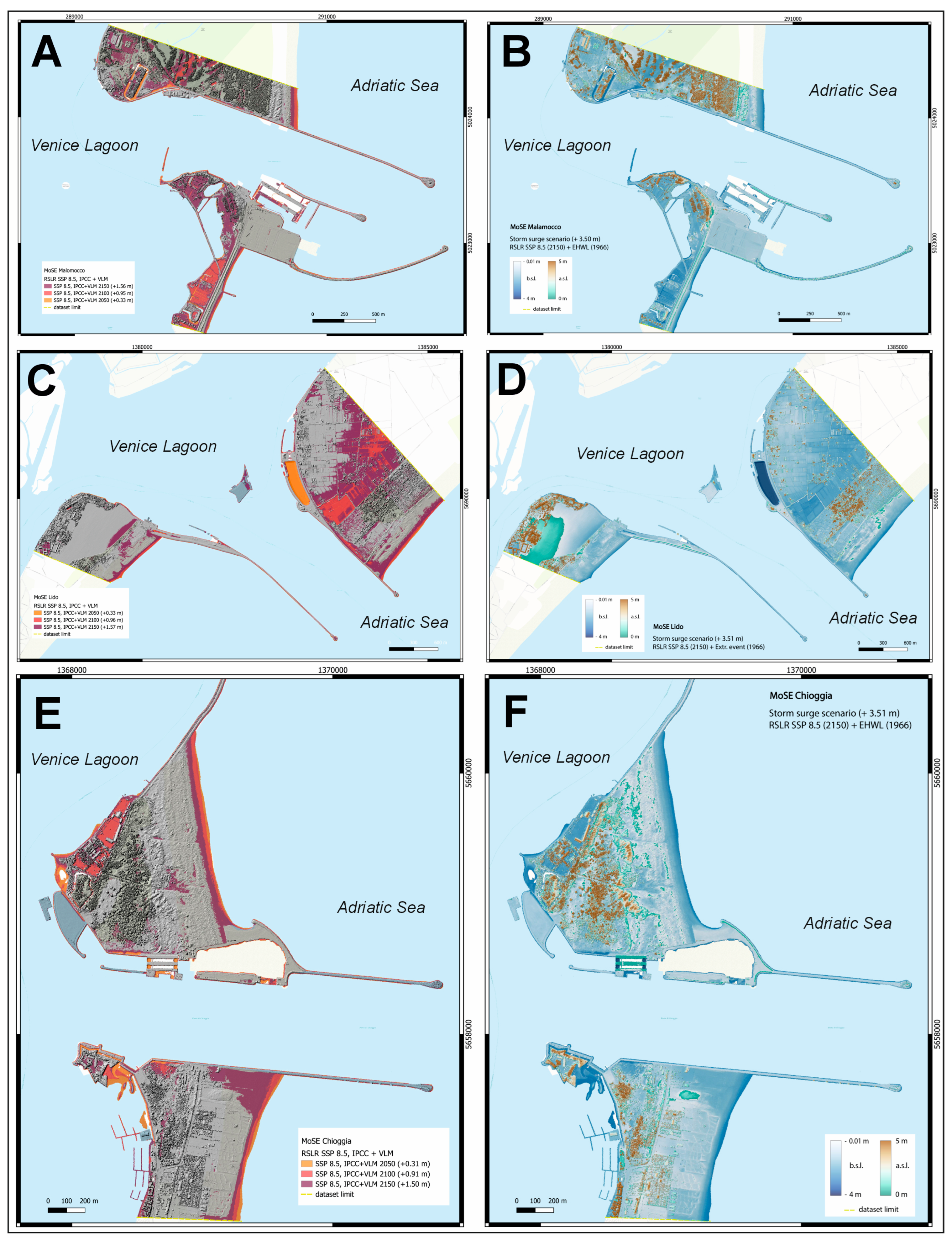
3.2.4. Areas 4, 5, and 6—The MoSE Barriers at the Lido, Malamocco, and Chioggia Inlets

The three inlets of the MoSE system at Malamocco (Figure 1 and Figure 7A,B), Lido (Figure 1 and Figure 7C,D), and Chioggia (Figure 1 and Figure 7E,F) are placed across the sedimentary coast that limits the lagoon from the open Adriatic Sea. The geodetic analysis for these areas shows they are affected by variable LS, also in coincidence with the MoSE structures, with mean values of 2.4–2.9 mm/yr. These rates are almost double compared to the more stable areas of the lagoon, such as the island of Venice, the Marco Polo airport, and St. Erasmo Island. This implies that for these three zones, the expected RSLR could be up to 1.53 m for 2150 for the SSP5-8.5 worst climatic scenario with an expected maximum loss of land of about 30% at Malamocco, 31% at Lido, and 22% at Chioggia. In MHWL conditions, like the 1966 event when the SL temporarily rose up to 1.94 m, the water may reach 3.47 m (benchmark 2023) above the zero reference at the Punta della Salute tide gauge station. In this case, the flooding surface would correspond to more than 70% (up to 78%) of land submergence (Table 2 and Table 4; Figure 7, Figure 10 and Figures S1.4–S1.6, S3 and S4.4–S4.6; and Supplementary Materials S5).

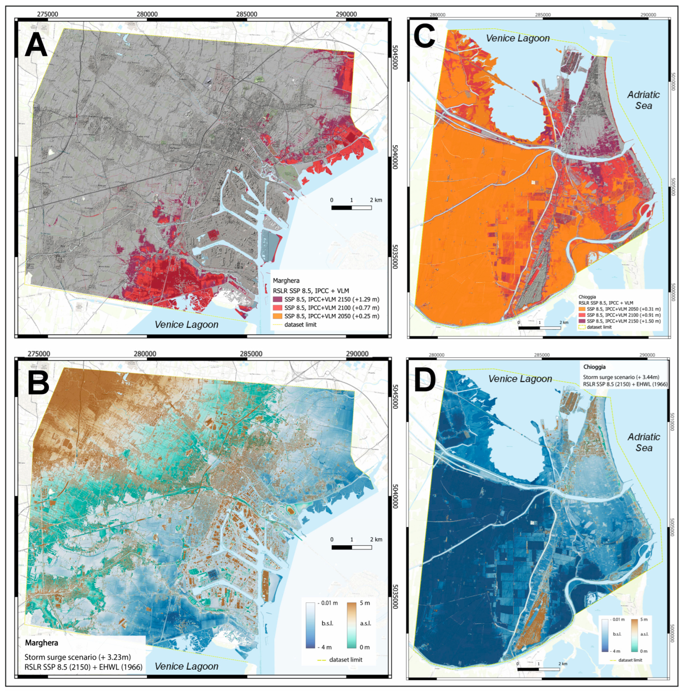
3.2.5. Area 7—Marghera Harbor

Marghera is located along the mainland facing the lagoon (Figure 1). It is divided into a residential district and a commercial port with important industrial infrastructures, which makes it an area of high economic value. The VLM for this area shows about 1 mm/yr of subsidence, and the expected RSLR could be up to 1.27 m in 2150 for the SSP5-8.5 worst climatic scenario (benchmark 2023). The flooding maps show that even if the rate of subsidence is quite low with respect to the other sectors of the lagoon, the area is still highly exposed to SLR. About 20 km2 of the area could be flooded in 2150 for the SSP5-8.5 climatic scenario. In the case of an MHWL event, the water would rise up to 3.21 m, with a flooded area of 44% (78 km2) (Table 2 and Table 4; Figure 8, Figure 10 and Figures S1.7, S3 and S4.7; and Supplementary Materials S5).

3.2.6. Areas 8, 9, and 10—The Lido Coastal Zone (Venice, Pellestrina, and Cavallino)

This area corresponds to the external sector of the lagoon, facing the North Adriatic Sea (Figure 1). It is characterized by low-lying sandy beaches with dunal systems, which are subjected to coastal erosion and retreat. The coast is often protected by the so-called “murazzi”, high concrete walls running parallel to the coasts to protect the inner zone from storm surges and extreme events. There are also defense systems, consisting of stone barriers built normally to the coastline, that facilitate sediment deposition, thus limiting coastal erosion. Among the three beaches, the expected RSLR in 2150 for the SSP5-8.5 scenario, considering 2023 as a benchmark, is greater in Lido Cavallino (up to 1.48 m) and lower in Lido Pellestrina (1.38 m), with a potential loss of land of about 20 km2, 18 of which occurs in Lido Cavallino. For an MHWL scenario, the water would rise between 3.34 and 3.42 m above the MSL. The three beaches would be highly affected by this extreme event and could be flooded by between a minimum of 58% in Lido Venezia and a maximum of 83% in Lido Cavallino (corresponding to about ⅔ of their surface) (Table 2 and Table 4; Figure 9, Figure 10 and Figures S1.8–S1.10, S3 and S4.8–S4.10; and Supplementary Materials S5).

3.2.7. Area 11—Chioggia

The village of Chioggia is located in the southern part of the lagoon (Figure 1). This area is characterized by low topography, rates of land subsidence up to 2.4 mm/yr, and complex coastal features, which makes it the most susceptible area of the Venice Lagoon to RSLR. Even in the low-emission climatic scenario SSP1-2.6, in 2150, the RSL is expected to rise 0.90 m (benchmark 2023), flooding about 72 km2 of land, corresponding to 75% of the area. While for the high-emission scenario SSP5-8.5, 81% of the investigated area, about 78 km2, could be submerged by the sea in the absence of any protection. Even worse is the MHWL conditions in 2150 for the SSP85 scenario, when 3.40 m of SLR (compared to 2023) could flood about 89 km2 of land (92% of the investigated area) (Table 2 and Table 4; Figure 8, Figure 10 and Figures S1.11, S3 and S4.11; and Supplementary Materials S5).

4. Discussion

To understand the changes that are taking place today in the Venice Lagoon and those that could take place in the coming decades due to the combined effects of LS and SLR, it is crucial to briefly figure out how the Lagoon has evolved throughout the Holocene. The origin of its formation can be dated to 6000–7000 yrs BP [25] as a consequence of the marine transgression after the Last Glacial Maximum. From geological and geomorphological proxies, [52] estimated that the RSL in the area of the Venice and the Grado-Marano Lagoons was at −9.3 ± 0.8 m at about 7.5 ka BP, at −5.5 ± 0.8 m around 6.6 ka BP, and about −3 m at 5.5 ka BP. During this period, the sea gradually rose, flooding the alluvial palaeo-plain of the northern Adriatic shelf and then forming the current lagoon systems [53,54,55,56]. However, as observed by [52], it is difficult to reconstruct the exact trend of the RSL in the Late Holocene in this area due to the variability in LS caused by sediment compaction in the different sectors of the lagoon. Besides the geological data, information on the historical evolution of the lagoon comes from ancient writers [57,58,59,60,61], who described the places in Roman or pre-Roman times (about 1500 BC–1500 AD). After 1000 AD, other authors, such as [62], provided additional information on the more recent evolution of the lagoon. In particular, around 1450 AD, [63] noted how the action of the Po, Adige, and Brenta rivers, contributed to the formation of the islands in the lagoon, favoring human settlements and the foundation of the city of Venice. Conversely, the coastal zone corresponding to the Lido began to shrink over time. These observations describe the continuous transformation of the lagoon, driven by the sedimentary contributions of rivers, the formation of dunes and shores, LS, changes in the SL, and human interventions with continuous adaptations. In addition to the slow transformations, extreme meteorological events reshaped the lagoon and its surroundings over time, like the 557 AD event [64]. The SLR in the Venice Lagoon is also evidenced by numerous submerged archaeological sites of maritime installations and buildings [2,65]. For example, the port of Metamauco (or Malamocco) was flooded in 1070 AD [2]. In 1535 AD, [62] it was measured at a depth of 19 ft (about 5.7 m), and in 1543, it was measured again at 20 ft of depth (about 6 m) [2,66]. In addition, a large port as well as several structures bearing with the sea level at the time of their construction (e.g., saltmarshes, fish tanks, and harbor installations), have been identified by [2] across the lagoon (Figure 11 and Figure 12). Recent studies [67,68] have identified other submerged structures in different areas of the lagoon, confirming that the SL continued to rise at greater values with respect to other areas of the Mediterranean coasts [65]. The current trend of SLR, as determined by instrumental data [6,7], is, therefore, in agreement with the historical evidence [2,67,68]. Based on these observations, it is reasonable to assume that such changes will continue to occur even more rapidly in the future, being accelerated by the increasing rates of SLR due to global warming [17]. Figure 11 shows the sea level prediction proposed by [13], which estimates an SLR for the Venice Lagoon of about 0.9 m during the last 3000 years and about 0.5 m since the Roman Age (e.g., 2000 ± 100 years BP), at a rate of about 0.25–0.30 mm y−1. The current position of the submerged archaeological structures was identified by [2,67,68] at a mean depth of 2.9 m (with maximum values of about 6 m) for the Roman age (between 1700 and 2100 years BP) and at a mean depth of −0.6 m for structures dated at 600–900 years BP [2]. By subtracting the glacial–hydro–isostatic contribution from the observed RSLC, we obtained the residual signal that can be attributed to the total VLM contribution due to tectonics, soil compaction, and anthropogenic causes, with an average subsidence rate of 1.6 ± 0.1 mm/yr. In the absence of any historical evidence of earthquakes able to suddenly displace the area along the vertical (see: https://emidius.mi.ingv.it/CPTI15-DBMI15/ (accessed on 20 February 2025)), this value can be used as representative of the velocity and trend of the VLM for the Venice Lagoon during the last 2100 years or so. This result is in agreement with the geodetic analysis carried out in this study and by [7,31,32], who estimated the VLM for the last decades and sea level trend for the last two centuries in this area. In particular, [65,69] analyzed the sea-level data collected by the tidal networks operating in the Mediterranean basin, highlighting a mean SLR at a rate of about 1.8 mm/yr for the last two to three centuries. The SL analysis for the Venice Lagoon shows a trend for the last century that is higher than the global and Mediterranean average [6,7,70], being influenced by VLM. During the last 38 years, the MSL trend observed at the tidal stations deployed across the lagoon was estimated at 4.8 ± 0.4 mm/yr, but with large variability between different locations that fell in the range of 2.8 ± 1.3 to 7.2 ± 0.7 mm/yr (Figure 5, Figure S2, and Table S1 in the Supplementary Materials). This difference can be mainly attributed to the spatial variability in VLM that affects this area, changing the local rate of RSLR (see Figure 4, Figure S2, and Table S1 in the Supplementary Materials). A comparison of the sea level trends with the tide gauges of Genoa and Trieste, which have among the longest records in the Mediterranean and are located in relatively stable areas from a tectonic point of view, shows the difference with the major trends observed in the lagoon, in particular, after 2000 AD (Figure 4). The SL at Trieste shows a trend of 1.08 mm/year in the period of 1875–2022 and 2.65 mm/year in the period of 2000–2022. Genoa, instead, has a trend of 1.10 mm/year in the period of 1884–2024 and 3.51 mm/year in the period of 2000–2024. The tidal data, therefore, show a greater and variable trend in the lagoon (see Figure S2 and Table S1 in the Supplementary Materials) that exceeds the regional trend [69]. Based on our revised IPCC AR6 projections up to 2150 for the RSLR for the current rate of land subsidence discussed above, assuming that the VLM rate will remain constant for this period, the Venice Lagoon will be exposed to critical high sea levels before 2150 (see Table 3 and Table 4; Figure 5, Figure 6, Figure 7, Figure 8, Figure 9 and Figure S4.1–S4.11; and Supplementary Materials S5). By combining our RSLR projections with the high-resolution topography derived from LiDAR data, the zones of the Venice Lagoon most exposed to flooding in the next decades were identified. These correspond to subsiding low-elevated areas where the exposure to flooding increases the lower their elevation above the MSL. Our analysis considered an area of about 350 km2, 112 and 139 of which can be potentially flooded in the SSP1-2.6 and SSP5-8.5 scenarios, respectively. In some places, such as Lido Cavallino, St. Erasmo Island, and the Marco Polo airport, the expected flooding is even favored by the lack of natural barriers, low elevated land, coastal erosion, soil compaction, land subsidence, and increasing anthropogenic pressure. All these factors contribute to accelerating the flooding process.

Implications for the MoSE System

In the last decades, climate change has dramatically increased the frequency of extremely high water level events (the so-called “acqua alta”) in the Venice Lagoon [66]. These events are favored when southerly winds (i.e., “scirocco”) combine with astronomical tides, seiches, and meteorological forcing, causing critical flooding both in the city of Venice and the lagoon [71,72,73]. The more frequently encountered high tides are up to 110 cm when about 12% of the historic city is flooded. It is worth noting that the worst events of “acqua alta”, when water levels exceed 140 cm above the zero reference level at the Punta della Salute tide gauge station, are now more frequent than in the past [72]. About 59% of the city is then submerged, seriously harming the safety of its inhabitants, human activities, and infrastructures [74]. Only in the past four years, between 2019 and 2023, about 58 events of tide amplitudes higher than 110 cm were recorded, compared to only 24 events that occurred in the period of 2009–2013 [74]. To mitigate these effects and the risk to the population, infrastructures, and cultural heritage, the Italian government realized the MoSE (Modulo Sperimentale Elettromeccanico, https://www.mosevenezia.eu/ (accessed on 20 February 2025)). This system, which cost about EUR 6.2 billion, consists of a set of submerged mobile barriers that are raised above the SL when high tides are up to 110 cm (closure threshold, see [71,75]) to temporarily close the connection of the Venice Lagoon with the Adriatic Sea, protecting the City of Venice from flooding. In 1984, the Italian government defined the objectives to safeguard Venice and its lagoon from SLR and “acqua alta” events. In 1995, the best technical solution was approved, and since 2023, this structure has successfully protected the lagoon. Based on the first report of the IPCC, published in 1994, a value of a global SLR of about 20 cm by 2100 was initially considered in the design of the MoSE. In 2007, the engineering project was then updated so that the MoSE could withstand up to 3 m of sea level difference between the open sea and the lagoon and a mean SLR of 60 cm in 2100 [74]. However, recent studies [7], which included the current VLM rate estimated by the GNSS network, projected RSLR values in 2100 for Venice in the RCP2.6 and RCP8.5 scenarios of the IPCC-AR5 Report released in 2014 at 60.3 ± 21.7 cm and 81.8 ± 25.8 cm, respectively. Our revised RSLR projections for the Venice Lagoon show values between 1.29 and 1.57 m in 2150 across the lagoon and between 1.50 m and 1.57 m along the three inlets of the MoSE, where the maximum rate of subsidence is occurring.
The MoSE was finally realized to work with a maximum SL of 3 m higher than today. However, during extreme storm surge events, the SL can temporarily rise to about 2 m (194 cm in 1966 and 187 cm in 2019 [76] or even up to 2.10 m [48]), thus leading to projected maximum sea levels over the threshold of 3 m. With these extreme SL values, the functionality of the MoSE will reasonably fail to protect the Venice Lagoon around 2100 (upper limit) or around 2030 (median likely range) for the SSP5-8.5 scenario, thus exposing the entire lagoon to flooding in the case of extremely high water level events.

5. Conclusions

In this study, we showed that land subsidence plays a fundamental role in increasing the future sea level variability in the Venice Lagoon. Our analysis, which incorporates the new geodetic rates of VLM in the SL projections, indicates that the revised estimates of SL for this area deviate from 11 cm to 37 cm with respect to the IPCC AR6 SSP8.5 scenarios (benchmark year 2023 AD). A total of about 139 km2 of land will possibly be submerged by 2150 in the case of a lack of protection systems for the mean RSLR values discussed above. This implies that in the following years, the Venice Lagoon will be increasingly exposed to marine flooding and coastal hazards. In the case of an MHWL due to the combination of storm surge and high tide, such as the 1966 event, the potential total flooded area would dramatically increase up to 226 km2 (64% of the investigated area). The potential effects of RSLR will be particularly relevant in the most low-lying areas of the lagoon, where land subsidence is more intense due to local factors. The above scenario poses critical conditions for human activities and the functionality of coastal infrastructures located in the lagoon, leading to their likely abandonment in the future, similar to what occurred in the past. The hazard implications for the population living in the Venice Lagoon should be considered by land planners and decision-makers by taking into account scenarios similar to those reported in this study for responsible coastal management. This is particularly relevant in the unlucky case of the unavailability of the protective barriers of the MoSE, with the SL possibly exceeding the maximum threshold of protection of 3 m against high water level episodes during extreme events. Such extreme episodes could happen around 2100 and likely well before 2150 for the SSP8.5 scenarios, thus exposing the entire lagoon to early flooding if the protection system is not updated to respond to expected changes. The multi-temporal RSLR projections and related flooding scenarios presented in this study are crucial for understanding the associated risks for the population and infrastructures, as well as for protecting the heritage sites in this area. This will push decision-makers to deal with these changes.

Supplementary Materials

The following supporting information can be downloaded at https://www.mdpi.com/article/10.3390/rs17050820/s1.

Author Contributions

Conceptualization, M.A., A.B., D.T. and T.A.; methodology, M.A., A.B., D.T. and T.A.; software, D.T. and T.A.; validation, T.A., D.T. and A.B.; formal analysis, C.T., E.S., D.T., T.A. and A.V.; investigation, M.A., D.T. and C.A.B.; resources, M.A., A.B. and C.A.B.; data curation, C.T., C.A.B., D.T. and T.A.; writing—original draft preparation, C.T., E.S., G.D. and M.A.; writing—review and editing, C.T., E.S., G.D., M.A., D.T., A.B., T.A. and A.F.; visualization, D.T.; supervision, M.A., T.A. and A.B.; funding acquisition, M.A. All authors have read and agreed to the published version of the manuscript.

Funding

This research was funded by MIUR PRIN2022_PE10_2022ZSMRXJ02.”Geomorphological and hydrogeological vulnerability of Italian coastal areas in response to sea level rise and marine extreme events. Acronym” GAIA” (P.I. Giuseppe Mastronuzzi, University of Bari Aldo Moro, Italy; Partners Marco Anzidei, INGV, Italy and Pietro Paolo Aucelli, University on Napoli Parthenope, Italy), under the umbrella of the Italian Ministry of Research. This study benefited from the methodology developed in the SAVEMEDCOASTS (Agreement number ECHO/SUB/2016/742473/PREV16) and SAVEMEDCOASTS-2 (Project number 874398) EU Projects (www.savemedcoasts.eu; www.savemedcoasts2.eu (accessed on 20 February 2025)).

Data Availability Statement

Copernicus Sentinel-1 IW SLC data for the PSI analysis were provided via the Copernicus Open Access Hub and processed by CTTC. Copernicus Sentinel-1 IW SAR data for the SBAS analysis were provided via, and processed in, ESA’s Geohazards Thematic Exploitation Platform (Geohazards TEP, or GEP), in the framework of the GEP Early Adopters Program and the Geohazards Lab initiative, the latter developed under the CEOS Working Group on Disasters. SAR data processing was carried out using the P-SBAS on-demand service developed and integrated by CNR-IREA in GEP. LiDAR data were provided by CO.RI.LA of Regione Veneto https://www.corila.it/en/ (accessed on 20 February 2025) and the Italian Ministry of the Environment at http://www.pcn.minambiente.it/viewer/ (accessed on 20 February 2025). GNSS data were retrieved, processed, and archived by the INGV Geodetic analysis data center. Tide gauge data of the sea level stations in the Venice Lagoon are freely available at www.mareografico.it and https://www.comune.venezia.it/it/content/centro-previsioni-e-segnalazioni-maree (accessed on 20 February 2025). Information and operability of the MoSE system are available at https://www.commissariostraordinariomose.it/ (accessed on 20 February 2025).

Acknowledgments

We are thankful to the Italian Ministry of the University and Research that funded this research under the project GAIA, contract no. PRIN2022_PE10_2022ZSMRXJ02. This research reflects the methodology applied in the SAVEMEDCOASTS (Agreement number ECHO/SUB/2016/742473/PREV16) and SAVEMEDCOASTS-2 (Project number 874398) EU Projects (www.savemedcoasts.eu; www.savemedcoasts2.eu (accessed on 20 February 2025)), both funded by DG ECHO. LiDAR data were made available by CO.RI.LA, https://www.corila.it/ (accessed on 20 February 2025), and the Italian Ministry of the Environment to generate the DEMs at 1 m resolution of the entire lagoon in the ItalGeo 2005 geoid model. We acknowledge Claudia Ferrari, of the Municipality of Venice, and Alvise Papa and Marco Favaro, of the tidal Center of the Municipality of Venice, for their kind collaboration. We acknowledge Franco Tonello, of the Marine Archaeology Research Venice Equipe, https://www.mar-ve.it/ (accessed on 20 February 2025), for the fruitful discussion on the submerged sector of the Venice lagoon. We wish to dedicate this study to the memory of Vincenzo Carbone, an esteemed professor of physics at the University of Calabria, who recently passed away. Beloved colleague, friend, and lover of the sea and nature, he will always be in our hearts.

Conflicts of Interest

The authors declare no conflict of interest.

Abbreviations

The following abbreviations are used in this manuscript:
AR6Sixth Assessment Report
CO.RI.LAConsortium for the coordination of research relating to the Venice lagoon system
DEMDigital Elevation Model
DSdistributed scatterer
DSMDigital Surface Model
EPSEnhanced Permanent Scatterer
FEflooding extension
GIAGlacial Isostatic Adjustment
GNSSGlobal Navigation Satellite System
InSARInterferometric Synthetic Aperture Radar
IPCCIntergovernmental Panel on Climate Change
LiDARLight Detection And Ranging
LSland subsidence
MHWLMaximum High Water Level
MoSEModulo Sperimentale Elettromeccanico
MSLmean sea level
MT-InSARMulti-Temporal Interferometric Synthetic Aperture Radar
PSPermanent Scatterers
RSLRrelative sea level rise
SARSynthetic Aperture Radar
SBSmall Baseline
SLsea level
SLRsea level rise
SSPShared Socioeconomic Pathway
UNESCOUnited Nations Educational, Scientific and Cultural Organization
VLMVertical Land Movement
ZMPSZero Mean sea level at Punta della Salute tide gauge station

References

  1. Doglioni, C. Some remarks on the origin of foredeeps. Tectonophysics 1993, 228, 1–20. [Google Scholar] [CrossRef]
  2. Canal Ernesto. Archeologia Della Laguna di Venezia; Cierre Edizioni: Sommacampagna, Italy, 2013; ISBN 9788883147906. [Google Scholar]
  3. City of Venice. Yearbook of Tourism Data 2019. City of Venice Tourism Department. 2021. Available online: https://www.comune.venezia.it/it/content/studi (accessed on 20 October 2022).
  4. Zanchettin, D.; Bruni, S.; Raicich, F.; Lionello, P.; Adloff, F.; Androsov, A.; Antonioli, F.; Artale, V.; Carminati, E.; Ferrarin, C.; et al. Sea-level rise in Venice: Historic and future trends (review article). Nat. Hazards Earth Syst. Sci. 2021, 21, 2643–2678. [Google Scholar] [CrossRef]
  5. Lionello, P.; Barriopedro, D.; Ferrarin, C.; Nicholls, R.J.; Orlić, M.; Raicich, F.; Reale, M.; Umgiesser, G.; Vousdoukas, M.; Zanchettin, D. Extreme floods of Venice: Characteristics, dynamics, past and future evolution (review article). Nat. Hazards Earth Syst. Sci. 2021, 21, 2705–2731. [Google Scholar] [CrossRef]
  6. Lionello, P.; Nicholls, R.J.; Umgiesser, G.; Zanchettin, D. Venice Flooding and Sea Level: Past Evolution, Present Issues, and Future Projections (Introduction to the Special Issue). Nat. Hazards Earth Syst. Sci. 2021, 21, 2633–2641. [Google Scholar] [CrossRef]
  7. Vecchio, A.; Anzidei, M.; Serpelloni, E.; Florindo, F. Natural variability and vertical land motion contributions in the mediterranean sea-level records over the last two centuries and projections for 2100. Water 2019, 11, 1480. [Google Scholar] [CrossRef]
  8. Carbognin, L.; Gambolati, G.; Johnson, A.I. (Eds.) Land Subsidence: Proceedings of the Sixth International Symposium on Land Subsidence; C.N.R.: Ravenna, Italy, 2000; Volume I–II. [Google Scholar]
  9. Cuffaro, M.; Riguzzi, F.; Scrocca, D.; Antonioli, F.; Carminati, E.; Livani, M.; Doglioni, C. On the geodynamics of the northern Adriatic plate. Rendiconti Lince Sci. Fis. Nat. 2010, 21, 253–279. [Google Scholar] [CrossRef]
  10. Falciano, A.; Anzidei, M.; Greco, M.; Trivigno, M.L.; Vecchio, A.; Georgiadis, C.; Patias, P.; Crosetto, M.; Navarro, J.; Serpelloni, E.; et al. The SAVEMEDCOASTS-2 webGIS: The Online Platform for Relative Sea Level Rise and Storm Surge Scenarios up to 2100 for the Mediterranean Coasts. J. Mar. Sci. Eng. 2023, 11, 2071. [Google Scholar] [CrossRef]
  11. Oppenheimer, M.; Bruce, G.; Jochen, H.; van de Wal, R.S.W.; Alexandre, A.; Abd-Elgawad, A.; Cai, R.; Cifuentes-Jara, M.; de Conto, R.; Tuhin, G.; et al. Sea Level Rise and Implications for Low Lying Islands, Coasts and Communities. In IPCC Special Report on the Ocean and Cryosphere in a Changing Climate; Pörtner, H.-O., Roberts, D.C., Masson-Delmotte, V., Zhai, P., Tignor, M., Poloczanska, E., Mintenbeck, K., Alegría, A., Nicolai, M., Okem, A., Eds.; IPCC: Geneva, Switzerland, 2019. [Google Scholar]
  12. Frederikse, T.; Landerer, F.W.; Caron, L.; Adhikari, S.; Parkes, D.; Humphrey, V.; Dangendorf, S.; Hogarth, P.; Zanna, L.; Cheng, L.; et al. The causes of sea-level rise since 1900. Nature 2020, 584, 393–397. [Google Scholar] [CrossRef]
  13. Mitrovica, J.X.; Tamisiea, M.E.; Davis, J.L.; Milne, G.A. Recent mass balance of polar ice sheets inferred from patterns of global sea-level change. Nature 2001, 409, 1026–1029. [Google Scholar] [CrossRef] [PubMed]
  14. Lambeck, K.; Woodroffe, C.D.; Antonioli, F.; Anzidei, M.; Gehrels, W.R.; Laborel, J.; Wright, A.J. Paleoenvironmental Records, Geophysical Modeling, and Reconstruction of Sea-Level Trends and Variability on Centennial and Longer Timescales. In Understanding Sea-Level Rise and Variability; Blackwell: Hoboken, NJ, USA, 2010; pp. 61–121. [Google Scholar]
  15. Lambeck, K.; Antonioli, F.; Anzidei, M.; Ferranti, L.; Leoni, G.; Scicchitano, G.; Silenzi, S. Sea level change along the italian coast during the Holocene and projections for the future. Quat. Int. 2011, 232, 250–257. [Google Scholar] [CrossRef]
  16. Jevrejeva, S.; Williams, J.; Vousdoukas, M.I.; Jackson, L.P. Future sea level rise is driving the worst case for extreme sea levels along the global coastline by 2100. Environ. Res. Lett. 2023, 18, 024037. [Google Scholar] [CrossRef]
  17. Fox-Kemper, B.; Hewitt, H.T.; Xiao, C.; Aðalgeirsdóttir, G.; Drijfhout, S.S.; Edwards, T.L.; Golledge, N.R.; Hemer, M.; Kopp, R.E.; Krinner, G.; et al. Ocean, Cryosphere, and Sea Level Change. In Climate Change: The Physical Science Basis. Contribution of Working Group I to the Sixth Assessment Report of the Intergovernmental Panel on Climate Change, Masson-Delmotte, V., Zhai, P., Pirani, A., Eds.; Cambridge University Press: Cambridge, UK, 2021. [Google Scholar]
  18. Cianflone, G.; Tolomei, C.; Brunori, C.A.; Dominici, R. InSAR Time Series Analysis of Natural and Anthropogenic Coastal Plain Subsidence: The Case of Sibari (Southern Italy). Remote Sens. 2015, 7, 16004–16023. [Google Scholar] [CrossRef]
  19. Anzidei, M.; Scicchitano, G.; Scardino, G.; Bignami, C.; Tolomei, C.; Vecchio, A.; Serpelloni, E.; De Santis, V.; Monaco, C.; Milella, M.; et al. Relative Sea-Level Rise Scenario for 2100 along the Coast of South Eastern Sicily (Italy) by InSAR Data, Satellite Images and High-Resolution Topography. Remote Sens. 2021, 13, 1108. [Google Scholar] [CrossRef]
  20. Shirzaei, M.; Bürgmann, R. Global climate change and local land subsidence exacerbate inundation risk to the San Francisco Bay Area. Sci. Adv. 2018, 4, eaap9234. [Google Scholar] [CrossRef]
  21. Brunori, C.A.; Murgia, F. Spatiotemporal Evolution of Ground Subsidence and Extensional Basin Bedrock Organization: An Application of Multitemporal Multi-Satellite SAR Interferometry. Geosciences 2023, 13, 105. [Google Scholar] [CrossRef]
  22. Doglioni, C. The Venetian Alps Thrust Belt. In Thrust Tectonics; McClay, K.R., Ed.; Chapman & Hall: London, UK, 1992; pp. 319–324. [Google Scholar]
  23. Doglioni, C.; Carminati, E. Structural styles and Dolomites field trip. Mem. Descr. Della Carta Geol. 2008, 82, 1–299. [Google Scholar]
  24. Gatto, P.; Carbognin, L. The Lagoon of Venice: Natural environmental trend and man-induced modification/La Lagune de Venise: L’évolution naturelle et les modifications humaines. Hydrol. Sci. Bull. 1981, 26, 379–391. [Google Scholar] [CrossRef]
  25. Pirazzoli, P.A. Sea Level Changes, The Last 20,000 Years; John Wiley & Sons: Hoboken, NJ, USA, 1996; p. 1996. [Google Scholar]
  26. Fontes, J.C.; Bortolami, G. Subsidence of the Venice Area During the Past 40,000 ys. Nature 1973, 244, 339–341. [Google Scholar] [CrossRef]
  27. Carbognin, L.; Teatini, P.; Tosi, L. Eustacy and land subsidence in the Venice Lagoon at the beginning of the new millennium. J. Mar. Syst. 2004, 51, 345–353. [Google Scholar] [CrossRef]
  28. Arca, S.; Beretta, G.P. Prima sintesi geodetico-geologica sui movimenti verticali del suolo nell’Italia Settentrionale (1897–1957). Boll. Geod. Sci. Aff. 1985, 44, 125–156. [Google Scholar]
  29. Carminati, E.; Di Donato, G. Separating natural and anthropogenic vertical movements in fast subsiding areas: The Po plain (N. Italy) case. Geophys. Res. Lett. 1999, 26, 2291–2294. [Google Scholar] [CrossRef]
  30. Fontana, A.; Vinci, G.; Tasca, G.; Mozzi, P.; Vacchi, M.; Bivi, G.; Salvador, S.; Rossato, S.; Antonioli, F.; Asioli, A.; et al. Hajdas, Lagoonal settlements and relative sea level during Bronze Age in Northern Adriatic: Geoarchaeological evidence and paleogeographic constraints. Quat. Int. 2017, 439, 17–36. [Google Scholar] [CrossRef]
  31. Tosi, L.; Carbognin, L.; Teatini, P.; Strozzi, T.; Wegmüller, U. Evidence of the present relative land stability of Venice, Italy, from land, sea, and space observations. Geophys. Res. Lett. 2002, 29, 3-1–3-4. [Google Scholar] [CrossRef]
  32. Serpelloni, E.; Cavaliere, A.; Martelli, L.; Pintori, F.; Anderlini, L.; Borghi, A.; Randazzo, D.; Bruni, S.; Devoti, R.; Perfetti, P.; et al. Surface velocities and strain-rates in the Euro-Mediterranean region: From massive GPS data processing. Front. Earth Sci. 2022, 10, 907897. [Google Scholar] [CrossRef]
  33. Massonnet, D.; Feigl, K.; Rossi, M.; Adragna, F. Radar interferometric mapping of deformation in the year after the Landers earthquake. Nature 1994, 369, 227–230. [Google Scholar] [CrossRef]
  34. Zebker, H.A.; Villasenor, J. Decorrelation in interferometric radar echoes. IEEE Trans. Geosci. Remote Sens. 1992, 30, 950–959. [Google Scholar] [CrossRef]
  35. Chen, C.W.; Zebker, H.A. Network approaches to two-dimensional phase unwrapping: Intractability and two new algorithms: Erratum. J. Opt. Soc. Am. A 2001, 18, 1192. [Google Scholar] [CrossRef]
  36. Ferretti, A.; Prati, C.; Rocca, F. Permanent scatterers in SAR interferometry. IEEE Trans. Geosci. Remote Sens. 2001, 39, 8–20. [Google Scholar] [CrossRef]
  37. Ferretti, A.; Fumagalli, A.; Novali, F.; Prati, C.; Rocca, F.; Rucci, A. A New Algorithm for Processing Interferometric Data-Stacks: SqueeSAR. IEEE Trans. Geosci. Remote. Sens. 2011, 49, 3460–3470. [Google Scholar] [CrossRef]
  38. Berardino, P.; Fornaro, G.; Lanari, R.; Sansosti, E. A new algorithm for surface deformation monitoring based on small baseline differential SAR interferograms. IEEE Trans. Geosci. Remote. Sens. 2002, 40, 2375–2383. [Google Scholar] [CrossRef]
  39. Hooper, A. A multi-temporal InSAR method incorporating both persistent scatterer and small baseline approaches. Geophys. Res. Lett. 2008, 35, 16. [Google Scholar] [CrossRef]
  40. Crosetto, M.; Monserrat, O.; Cuevas-González, M.; Devanthéry, N.; Crippa, B. Persistent Scatterer Interferometry: A review. ISPRS J. Photogramm. Remote Sens. 2016, 115, 78–89. [Google Scholar] [CrossRef]
  41. Hooper, A.; Bekaert, D.; Spaans, K.; Arıkan, M. Recent advances in SAR interferometry time series analysis for measuring crustal deformation. Tectonophysics 2012, 514-517, 1–13. [Google Scholar] [CrossRef]
  42. Casu, F.; Manzo, M.; Lanari, R. A quantitative assessment of the SBAS algorithm performance for surface deformation retrieval from DInSAR data. Remote Sens. Environ. 2006, 102, 195–210. [Google Scholar] [CrossRef]
  43. Ferrarin, C.; Lionello, P.; Orlić, M.; Raichic, F.; Salvadori, G. Venice as a paradigm of coastal flooding under multiple compound drivers. Sci. Rep. 2022, 12, 5754. [Google Scholar] [CrossRef] [PubMed]
  44. Barzaghi, R.; Borghi, A.; Carrion, D.; Sona, G. Refining the estimate of the Italian quasi-geoid. Boll. Geod. E Sci. Affin. 2007, 66, 145–159. [Google Scholar]
  45. Albertella, A.; Barzaghi, R.; Carrion, D.; Maggi, A. The joint use of gravity data and GPS/levelling undulations in geoid estimation procedures. Boll. Geod. E Sci. Affin. 2008, 67, 49–59. [Google Scholar]
  46. Yunus, A.P.; Avtar, R.; Kraines, S.; Yamamuro, M.; Lindberg, F.; Grimmond, C.S.B. Uncertainties in Tidally Adjusted Estimates of Sea Level Rise Flooding (Bathtub Model) for the Greater London. Remote Sens. 2016, 8, 366. [Google Scholar] [CrossRef]
  47. Gallien, T.W.; Sanders, B.F.; Flick, R.E. Urban Coastal Flood Prediction: Integrating Wave Overtopping, Flood Defenses and Drainage. Coast. Eng. 2014, 91, 18–28. [Google Scholar] [CrossRef]
  48. Cavaleri, L.; Bajo, M.; Barbariol, F.; Bastianini, M.; Benetazzo, A.; Bertotti, L.; Chiggiato, L.; Ferrarin, C.; Umgiesser, G.; Trincardi, F. The 2019 Flooding of Venice and Its Implications for Future Predictions. Oceanography 2020, 33, 42–49. [Google Scholar] [CrossRef]
  49. Seenath, A.; Wilson, M.; Miller, K. Hydrodynamic versus GIS Modelling for Coastal Flood Vulnerability Assessment: Which Is Better for Guiding Coastal Management? Ocean Coast. Manag. 2016, 120, 99–109. [Google Scholar] [CrossRef]
  50. Anderson, T.R.; Fletcher, C.H.; Barbee, M.M.; Romine, B.M.; Lemmo, S.; Delevaux, J.M.S. Modeling Multiple Sea Level Rise Stresses Reveals up to Twice the Land at Risk Compared to Strictly Passive Flooding Methods. Sci. Rep. 2018, 8, 14484. [Google Scholar] [CrossRef] [PubMed]
  51. Gao, X.-J.; Wang, X.-Y. Impacts of Global Warming and Sea Level Rise on Service Life of Chloride-Exposed Concrete Structures. Sustainability 2017, 9, 460. [Google Scholar] [CrossRef]
  52. Vacchi, M.; Marriner, N.; Morhange, C.; Spada, G.; Fontana, A.; Rovere, A. Multiproxy assessment of Holocene relative sea-level changes in the western mediterranean: Sea-level variability and improvements in the definition of the isostatic signal. Earth Sci. Rev. 2016, 155, 172–197. [Google Scholar] [CrossRef]
  53. Trincardi, F.; Correggiari, A.; Roveri, M. Late Quaternary transgressive erosion and deposition in a modern epicontinental shelf: The Adriatic semienclosed basin. Geo-Marine Lett. 1994, 14, 41–51. [Google Scholar] [CrossRef]
  54. Trincardi, F.; Cattaneo, A.; Asioli, A.; Correggiari, A.; Langone, L. Stratigraphy of the late-Quaternary deposits in the central Adriatic basin and the record of short-term climatic events. Mem. Ist. Ital. Idrobiol. 1996, 55, 39–70. [Google Scholar]
  55. Correggiari, A.; Field, M.; Trincardi, F. Late Quaternary transgressive large dunes on the sediment-starved Adriatic shelf. Geol. Soc. Lond. Spec. Publ. 1996, 117, 155–169. [Google Scholar] [CrossRef]
  56. Storms, J.E.A.; Weltje, G.J.; Terra, G.J.; Cattaneo, A.; Trincardi, F. Coastal dynamics under conditions of rapid sea-level rise: Late Pleistocene to Early Holocene evolution of barrier–lagoon systems on the northern Adriatic shelf (Italy). Quat. Sci. Rev. 2008, 27, 1107–1123. [Google Scholar] [CrossRef]
  57. Strabone. Geografia. L’Italia; Biraschi, A.M., Ed.; Libro V; BUR (Biblioteca Universale Rizzoli): Milano, Italy, 1988; ISBN 88-17-16687-1. [Google Scholar]
  58. Pliny the Elder. Natural History. Volume III, Chapter XVI. Available online: https://www.perseus.tufts.edu/ (accessed on 20 February 2025).
  59. 54 Titus Livius Ab urbe condita, lib.X Storia di Roma Dalla Sua Fondazione; BUR: Milano, Italy, 2010; Volume 10, ISBN 978-88-17-17168-7.
  60. Cassiodorus. Roma Immaginaria; Laccetti, D., Ed.; Arbor Sapientiae: Roma, Italy, 2014. [Google Scholar]
  61. Vitruvius The Ten Books on Architecture; Morgan, M.H., Translator; Harvard University Press: Cambridge, MA, USA, 1914; ISBN 978-0-486-20645-5. [Google Scholar]
  62. Sabbadino, C. Discorsi Sopra la Laguna; Cessi, R., Ed.; Ferrari: Venezia, Italy, 1930; Volume II. [Google Scholar]
  63. Morosini, P. Memoria storica intorno alla Repubblica di Venezia; Palese, C., Ed.; Nella Stamperia di Carlo Palese: Vienna, Italy, 1796; 816p. [Google Scholar]
  64. Diacono, P. Storia dei Longobard; Edizione TEA: Tokyo, Japen, 1988. [Google Scholar]
  65. Anzidei, M.; Lambeck, K.; Antonioli, F.; Furlani, S.; Mastronuzzi, G.; Serpelloni, E.; Vannucci, G. Coastal structure, sea-level changes and vertical motion of the land in the Mediterranean. Geol. Soc. Lond. Spec. Publ. 2014, 388, 453–479. [Google Scholar] [CrossRef]
  66. Adami, A.; Baschieri, P. Gran porto fa gran laguna. In Atti. Classe di Scienze Fisiche, Matematiche e Naturali; Tomo 153, Fascicolo 1; Istituto Veneto di Scienze: Venice, Italy, 1994. [Google Scholar]
  67. Madricardo, F.; Bassani, M.; D’acunto, G.; Calandriello, A.; Foglini, F. New evidence of a Roman road in the Venice Lagoon (Italy) based on high resolution seafloor reconstruction. Sci. Rep. 2021, 11, 13985. [Google Scholar] [CrossRef] [PubMed]
  68. Tonello, F.; Romana, T. Canale San Felice; Associazione culturale W San Marco: Venezia, Italy, 2019. [Google Scholar]
  69. Wöppelmann, G.; Marcos, M. Coastal sea level rise in southern Europe and the non-climate contribution of vertical land motion. J. Geophys. Res. 2012, 117, C01007. [Google Scholar] [CrossRef]
  70. Vecchio, A.; Anzidei, M.; Serpelloni, E. Sea level rise projections up to 2150 in the northern Mediterranean coasts. Environ. Res. Lett. 2023, 19, 014050. [Google Scholar] [CrossRef]
  71. Giupponi, C.; Bidoia, M.; Breil, M.; Di Corato, L.; kumar Gain, A.; Leoni, V.; Minooei Fard, B.; Pesenti, R.; Umgiesser, G. Boon and burden: Economic performance and future perspectives of the Venice flood protection system. Reg. Environ. Chang. 2024, 24, 44. [Google Scholar] [CrossRef]
  72. Alberti, T.; Anzidei, M.; Faranda, D.; Vecchio, A.; Favaro, M.; Papa, A. Dynamical diagnostic of extreme events in Venice lagoon and their mitigation with the MoSE. Sci. Rep. 2023, 13, 10475. [Google Scholar] [CrossRef] [PubMed]
  73. Faranda, D.; Ginesta, M.; Alberti, T.; Coppola, E.; Anzidei, M. Attributing Venice Acqua Alta events to a changing climate and evaluating the efficacy of MoSE adaptation strategy. Npj Clim. Atmospheric Sci. 2023, 6, 181. [Google Scholar] [CrossRef]
  74. Anzidei, M.; Alberti, T.; Vecchio, A.; Loizidou, X.; Orthodoxou, D.; Serpelloni, E.; Falciano, A.; Ferrari, C. Sea level rise and extreme events along the Mediterranean coasts: The case of Venice and the awareness of local population, stakeholders and policy makers. Rendiconti Lince Sci. Fis. Nat. 2024, 35, 359–370. [Google Scholar] [CrossRef]
  75. Venezia, C.D. Durata e Frequenza Media Della Maree. 2022. Available online: https://www.comune.venezia.it/it/content/durata-media-delle-maree2 (accessed on 20 October 2024).
  76. Venezia, C.D. Distribuzione annuale alte e basse maree. 2020. Available online: https://www.comune.venezia.it/it/content/distribuzione-annuale-delle-alte-maree-110-cm (accessed on 20 October 2024).
Figure 1. The Venice Lagoon (Northern Italy). The red polygons show the 11 selected areas for the detailed RSLR scenarios.
Remotesensing 17 00820 g001
Figure 2. (A) Comparison between SAR and GNSS Up velocity, with the relative error bars estimated at the geodetic stations located across the lagoon and the surrounding area. The plot shows the difference between the vertical GNSS and InSAR velocities with respect to the perfect values coincidence (red dashed line) at each considered GNSS station. The closer the differences are to the bisector (red dashed line), the more similar the GNSS and InSAR vertical velocities. (B) Difference values of the Up velocity between InSAR and GNSS stations. The horizontal green lines show the range of uncertainty in InSAR (±2 mm/yr).
Remotesensing 17 00820 g002
Figure 3. EPS solution of the ground vertical velocity map over the Venice Lagoon for the time span of 22 June 2017–25 October 2023, calibrated on the local GNSS network. The location of the GNSS and tide gauge stations used in this study are reported on the map.
Remotesensing 17 00820 g003
Figure 4. Sea level rate (mm/yr) at the tidal stations located in the Venice Lagoon (including the historical Punta della Salute, Genova, and Trieste, for comparison—green symbols). The horizontal line marks the average SL rate inside the lagoon (4.8 ± 0.4 mm/yr). The red and black symbols refer to higher- and lower-than-average values, respectively.
Remotesensing 17 00820 g004
Figure 5. Area 1, Venice Island. Expected extension of flooding in 2050, 2100, and 2150 for the SSP5-8.5 emission scenarios and 1.4 mm/yr of land subsidence (see color scale). (A) The maximum expected RSLR is 1.35 m in 2150 (benchmark year 2018) with a loss of land of 0.63 km2. (B) The maximum potential flooding scenarios for 2150 AD in the SSP5-8.5 climatic projection for a maximum WL of 1.94 m, corresponding to the storm surge of 1966 AD and to a projected MHWL of 3.29 m (see Table 2, Table 3 and Table 4 and the Supplementary Materials for details).
Remotesensing 17 00820 g005
Figure 6. Area 2, S. Erasmo (A,B), and Area 3, Marco Polo airport (C,D). Expected extension of land flooding in 2050, 2100, and 2150 for the SSP5-8.5 emission scenarios (see color scale). The expected maximum RSLR in 2150 is up to 1.35 m in (A) and 1.33 m in (C) (benchmark year 2009). (B,D) Maximum potential flooding scenarios for 2150 AD in the SSP5-8.5 climatic projection for a maximum WL of 1.94 m, corresponding to the storm surge of 1966 AD and to a projected MHWL of 3.29 m in (B) and 3.27 m in (D), respectively (see Table 2, Table 3 and Table 4 and the Supplementary Materials for details).
Remotesensing 17 00820 g006
Figure 7. Area 4, MoSE inlet Malamocco (A,B), Area 5, MoSE inlet Lido (C,D), and Area 6, MoSE inlet Chioggia (E,F). Expected extension of land flooding in 2050, 2100, and 2150 for the SSP5-8.5 emission scenarios (see color scale). (A,C,E) The maximum expected RSLR in 2150 is up to 1.56 m in (A) (2.8 mm/yr of LS); 1,57 m in (C) (2.9 mm/yr of LS), and 1.5 m in (E) (2.4 mm/yr of LS) (benchmark year 2008). (B,D,F) Maximum potential flooding scenarios for 2150 AD in the SSP5-8.5 climatic projection for a maximum WL of 1.94 m, corresponding to the storm surge of 1966 AD and to a projected MHWL of 3.50 m in (A) and 3.51 m in (D,F) (see Table 2, Table 3 and Table 4 and the Supplementary Materials for details).
Remotesensing 17 00820 g007
Figure 8. Area 7, Marghera (A,B), and Area 11, Chioggia (C,D). Expected extension of land flooding in 2050, 2100, and 2150 AD for the SSP5-8.5 emission scenarios (see color scale). The maximum expected RSLR in 2150 is up to 1.29 m in (A) and 1.50 m in (C) (benchmark year 2008) for 0.9 and 2.4 mm/yr of LS, respectively (see color scale). (B,D) The maximum potential flooding scenarios for 2150 AD in the SSP5-8.5 climatic projection for a maximum WL of 1.94 m, corresponding to the storm surge of 1966 AD and to a projected MHWL of 3.23 m in (B) and 3.44 m in (D) (see Table 2, Table 3 and Table 4 and the Supplementary Materials for details).
Remotesensing 17 00820 g008
Figure 9. Area 8, Lido Cavallino (A,B), Area 9, Lido Pellestrina (C,D), and Area 10, Lido Venezia (E,F). The colors report the expected extension of land flooding in 2050, 2100, and 2150 for the SSP5-8.5 emission scenarios. The maximum expected RSLR in 2150 is up to 1.51 m in (A), 1.40 m in (C), and 1.44 m in (E) (benchmark year 2009) for 2.5, 1.7, and 2.0 mm/yr of LS, respectively (see color scale). (B,D,E) Maximum potential flooding scenarios for 2150 AD in the SSP5-8.5 climatic projection for a maximum WL of 1.94 m, corresponding to the storm surge of 1966 AD and to a projected MHWL of 3.45 m in (A), 3.34 m in (D), and 3.38 m in (F) (see Table 2, Table 3 and Table 4 and the Supplementary Materials for details).
Remotesensing 17 00820 g009
Figure 10. Percentage of the expected flooding extension for 2050, 2100, and 2150 AD for each one of the 11 selected areas for the SSP1-2.6, SSP3-7.0, and SSP5-8.5 emission scenarios. The most exposed areas are Chioggia in the southern sector of the lagoon and the Marco Polo airport.
Remotesensing 17 00820 g010
Figure 11. Sea level prediction for the last 3 Kyrs BP and up to 2150 AD (black curve) for the Venice Lagoon according to the model by [15] and this study, projected against the age and current elevation of a set of submerged archaeological indicators bearing the sea level, as reported in [2,67,68]. The blue horizontal line is the present-day sea level. Depth variability is dependent on the age of the structure and the local velocities of land subsidence. It is worth noting the projected sharp SLR predicted after 2000 AD and up to 2150 with respect to its overall stability during the last centuries.
Remotesensing 17 00820 g011
Figure 12. Historical evidence of land flooding due to subsidence, SLR, and erosion. (A) Sketch of the causes and effects of the progressive RSLR with archaeological evidence of inland relocation of buildings and submersion. (B) Madonna del Monte island, built along the San Giacomo Channel in 1303 AD (High Medieval Age). The island was abandoned by mid-1900 AD after a destructive storm surge (photo by Marco Anzidei).
Remotesensing 17 00820 g012
Table 1. VLM rates from GNSS data in the Venice Lagoon. The station positions, rate of the vertical motion (Vup), uncertainties at the 2-sigma level (Sup), and duration of the recording period (time) are reported in the table.
Station Name LatLonVup (mm/yr) 1Sup (mm/yr)Time (Years)
CAVA45.479412.5827−2.790.409.62
CGIA45.206512.2655−2.210.3312.85
MIRA45.497612.0954−1.180.3110.44
MSTR45.490412.2386−2.860.526.74
PSAL45.430712.3365−1.070.369.02
VEAR45.437912.3578−2.291.074.56
VEN145.430612.3541−1.410.2315.57
1 Mean Vup: −1.97 ± 0.46 mm/yr.
Table 2. Mean subsidence rates (Vup) for each one of the investigated areas (see also Figures S1.1–S1.11 in the Supplementary Materials).
SiteMean of All
Areas
MoSE
Chioggia
ChioggiaVeniceSt. Erasmo
Island
Marghera
Vup
(mm/yr)
−1.93−2.4−2.4−1.4−1.4−0.9
SiteMoSE
Malamocco
Lido
Venezia
Lido
Cavallino
Lido
Pellestrina
MoSE
Lido
Airport
Vup
(mm/yr)
−2.8−2.0−2.5−1.7−2.9−1.2
Table 3. Relative sea level projections for the SSP1-2.6, SSP3-7.0, and SSP5-8.5 scenarios for 2050, 2100, and 2150 with respect to 2023, for the Venice lagoon. For the full description of the uncertainties, see Supplementary Materials S5.
IPCC ScenarioYear
AD
IPCC SLR
(cm)
VLM (InSAR)
(cm)
RSLR
(cm)
SSP1-2.62050182–820–26
2100417–2248–63
21506011–3771–97
SSP3-7.02050202–822–28
2100607–2267–82
215010011–37113–139
SSP5-8.52050212–823–29
2100697–2276–91
215011611–37127–153
Table 4. Expected RSLR (m) and flooding extension (FE, km2) for the 11 selected areas of the Venice Lagoon in 2050, 2100, and 2150 AD for the SSP1-2.6 (a), SSP3-7.0, (b) and SSP5-8.5 (c) emission scenarios (values refer to the benchmark year).
2050 AD2100 AD2150 AD
IDAreaRSLRFERSLRFERSLRFE
(a) SSP1–2.6 Scenario
1Venice Island0.230.010.530.040.790.10
2St. Erasmo 0.230.330.531.100.791.92
3Airport0.236.970.529.150.7711.86
4MoSE Malamocco0.300.040.670.091.000.16
5MoSE Lido 0.300.090.680.171.010.41
6MoSE Chioggia0.280.050.630.090.940.16
7Marghera0.224.510.497.830.7311.90
8Lido Cavallino0.281.480.646.050.9513.11
9Lido Pellestrina0.250.020.570.070.840.19
10Lido Venezia0.260.070.590.190.880.38
11Chioggia0.2857.880.6366.740.9472.03
(b) SSP3–7.0 Scenario
1Venice Island0.250.010.720.081.210.47
2St. Erasmo 0.250.370.721.721.212.82
3Airport0.257.110.7111.281.1914.01
4MoSE Malamocco0.320.040.860.121.420.31
5MoSE Lido 0.320.100.870.261.430.97
6MoSE Chioggia0.300.050.820.131.360.27
7Marghera0.244.720.6811.151.1517.99
8Lido Cavallino0.301.640.8310.661.3717.22
9Lido Pellestrina0.270.250.760.141.260.61
10Lido Venezia0.280.080.780.301.300.96
11Chioggia0.3058.310.8270.471.3676.73
(c) SSP5–8.5 Scenario
1Venice Island0.260.010.810.121.350.63
2St. Erasmo 0.260.390.811.971.353.05
3Airport0.267.170.8012.091.3314.56
4MoSE Malamocco0.330.040.950.141.560.37
5MoSE Lido 0.330.100.960.351.571.19
6MoSE Chioggia0.310.060.910.151.500.32
7Marghera0.254.820.7712.481.2920.47
8Lido Cavallino0.311.720.9212.581.5118.13
9Lido Pellestrina0.280.030.850.231.400.72
10Lido Venezia0.290.080.870.371.441.22
11Chioggia0.3158.670.9171.671.5078.13
Disclaimer/Publisher’s Note: The statements, opinions and data contained in all publications are solely those of the individual author(s) and contributor(s) and not of MDPI and/or the editor(s). MDPI and/or the editor(s) disclaim responsibility for any injury to people or property resulting from any ideas, methods, instructions or products referred to in the content.

