Abstract
This paper addresses the deployment of a multi-functional radar network (MFRN) in complex regions that may exhibit non-connectivity, holes, or concave shapes, utilizing multi-objective particle swarm optimization (MOPSO). Unlike traditional approaches that rely on constraint-handling techniques, the proposed methodology leverages the unique characteristics of polygonal deployment regions to enhance deployment efficiency. Specifically, for the aforementioned complex deployment regions, a region decomposition approach based on convex partitioning is proposed. This approach allows for the decomposition of complex regions into multiple non-overlapping convex subregions. Moreover, for convex deployment regions or subregions, we propose a coordinate transformation approach to eliminate the constraints introduced by the shape of the convex region. By combining the above approaches, we introduce a novel MOPSO based on decomposition and transformation, named MOPSO-DT. This algorithm aims to optimize MFRN deployment in these challenging environments. Experimental results demonstrate the superiority of the MOPSO-DT algorithm over two existing algorithms across a variety of deployment cases, highlighting its enhanced efficiency, effectiveness, and stability. These findings indicate that the proposed algorithm is well suited for optimizing MFRN deployment in complex, irregular regions, offering significant improvements in performance compared to conventional methods.
1. Introduction
In recent years, radar networks have garnered considerable attention from the research community, primarily due to their superior performance compared to monostatic radar [1]. Given the excellent performance of networked radars and their potential to perform multiple tasks simultaneously, multi-functional radar networks (MFRNs) have been substantially explored [2,3,4]. However, the deployment process is arduous. First, the placement of MFRNs critically impacts their performance, necessitating considerable effort in their deployment [3,4,5,6,7,8,9,10,11,12,13,14,15,16,17,18,19]. Second, the location requirements for MFRNs vary depending on the specific tasks being undertaken, and these requirements often contradict one another [2,5,6,20]. Third, researchers are tasked with resolving these challenges while minimizing algorithmic complexity, especially in time-sensitive and computationally intensive applications [15,18,21].
A prevalent approach to addressing these challenges is to model the MFRN deployment problem as a multi-objective optimization problem and solve it using multi-objective heuristic algorithms, such as MOPSO [15,16,17,22]. However, the majority of existing studies concentrate on deployment regions characterized by relatively simple geometries, such as rectangles or cubes, without considering the complexity of deployment regions affected by obstacles or other constraints. This indicates that current research has insufficiently addressed the constraints imposed by irregular deployment regions, particularly mathematically complex polygons that exhibit non-connectivity, holes, or concave shapes, which are not uncommon in engineering practice. Furthermore, the emergence of complex deployment regions is likely to pose additional challenges for MFRN deployment. Therefore, this paper aims to explore this issue.
1.1. Overview
Research on the deployment problem can be broadly classified into two categories according to its solution approach. The first category aims to develop analytical solutions to deployment problems under various criteria by analyzing the evaluation criteria for deployment schemes, particularly concerning the placement of each node, through meticulous theoretical derivation. The second category involves arithmetic solutions to MFRN deployment problems, which involves formulating the MFRN deployment problems and developing optimization algorithms to obtain solutions. The former approach is more rigorous and computationally intensive, whereas the latter encompasses a broader range of applications. The following subsections present overviews of these two approaches.
1.1.1. Analytical Solutions to the MFRN Deployment Problem
The initial researchers were primarily concerned with the analytical solutions to MFRN deployment problems. Numerous studies have investigated optimal node deployment criteria for radar networks that perform a variety of tasks. In the framework of a multiple-input multiple-output (MIMO) noise radar network, a node deployment criterion that focuses on enhancing target location estimation accuracy was proposed [7]. A node deployment criterion was proposed to maximize worst-case intrusion detectability for a bi-static radar network. The network functions as a set of sensors tasked with providing belt-barrier coverage [8]. In the framework of a MIMO radar network performing region surveillance, a node deployment criterion was based on the principles of the Fisher information distance, as derived from an information geometric perspective [9]. In the framework of a sensor network performing region monitoring tasks, a node deployment criterion was proposed to optimize sensor-source geometry by maximizing the determinant of the corresponding Fisher information matrix [10]. The approach takes into account the communication distance between sensors within a rectangular region. In the framework of an MFRN performing detection and communication tasks simultaneously, a node deployment criterion was proposed to maximize the signal-to-interference-plus-noise ratio of each channel while minimizing the geometric dilution of precision (GDOP) [3]. In the framework of a MIMO radar network performing localization tasks, a node deployment criterion based on the Cramer–Rao lower bound (CRLB) of localization accuracy was proposed from the perspective of dynamic game theory [11]. The aforementioned works have established a set of evaluation criteria for node deployment schemes when radar networks perform a variety of tasks in diverse scenarios. While these criteria are undoubtedly instructive, they are not readily applicable in practice. On the one hand, the evaluation criteria are computationally intensive. On the other hand, the constraints imposed by these criteria are relatively stringent.
1.1.2. Arithmetic Solutions to the MFRN Deployment Problem
With respect to the algorithms employed to address deployment problems, they can be further classified into two primary categories: those that employ deterministic optimization methods and those that utilize stochastic optimization methods. Indeed, the latter category includes heuristic algorithms.
In the domain of research addressing the MFRN deployment problem through deterministic optimization approaches, the studies are relatively few. For the detection performance of MIMO radar networks, a joint optimization method employing a water-filling-type algorithm was proposed to optimize node location and power allocation [12]. Meanwhile, another joint optimization method for node location and power allocation was presented, with an objective function aimed at maximizing the signal-to-noise ratio (SNR). The method involves discretizing the rectangular deployment region into a set of points and solving it through a graph theoretical framework [13]. In the framework of the localization performance of MIMO radar networks, an algorithm based on the alternating direction method of multipliers was proposed for solving the deployment scheme with the CRLB of target localization accuracy as the objective function [14]. While these methods are undoubtedly valuable, it is worth emphasizing that none of them takes into account the constraints imposed by irregular deployment regions.
Meanwhile, research addressing the MFRN deployment problem through stochastic optimization approaches is particularly popular. To enhance the localization performance of a passive MIMO radar network, the deployment scheme was optimized using a stochastic optimization algorithm known as the genetic algorithm [16]. In order to simultaneously enhance the detection and localization performance of a passive MFRN, researchers employed effective coverage and GDOP as optimization metrics. They proposed a novel multi-objective heuristic algorithm, the multi-objective neighborhood search algorithm with multi-neighborhood structure, to optimize the deployment scheme [15]. In another study focused on the surveillance and localization capabilities of passive MFRNs, detection probability and GDOP were used as objective functions. The researchers addressed the interdependence between these two objective functions by introducing a novel algorithm, named self-constrained multi-objective particle swarm optimization, to optimize the deployment scheme [5]. In terms of detection and tracking performance, the researchers simultaneously examined detection probability and the weighted sum of localization errors as performance indicators and proposed a modified non-dominated sorting genetic algorithm based on Pareto theory to optimize the deployment scheme [6]. However, these studies are based on the assumption that the deployment region is a regular rectangular (or cubic) space, overlooking the impact of deployment region shape on deployment problems.
Concurrently, research on irregular deployment regions has gradually garnered the attention of the academic community. To enhance the detection performance of netted MIMO radar systems with mixed baselines, a particle swarm optimization (PSO) algorithm featuring a novel search strategy, referred to as Cluster-Constrained PSO, was proposed. The authors claimed that this algorithm can effectively handle various constraints, including those associated with irregular deployment regions [17]. In the framework of an MIMO radar network engaging in multiple target-tracking tasks, a node deployment algorithm comprising a deterministic optimization approach, semi-definite programming, and a stochastic optimization method, namely improved particle swarm optimization-tabu search, was proposed [18]. Within the deployment region, a non-deployable circular region is identified. This challenge is further transformed into a chance constraint and addressed through the Latin hypercube sampling-based stochastic optimization method. However, the aforementioned studies equate the constraints imposed by complex deployment regions with general constraints, rather than leveraging specific characteristics of the deployment region to propose more targeted solution methods.
In summary, the aforementioned studies concentrate on applications that address MFRN deployment issues in regular regions, while only a few studies explore complex deployment regions in general. Nevertheless, these studies on complex deployment regions remain relatively insufficient, given the significant challenge of addressing these constraints.
1.2. Motivation
This paper is primarily motivated by engineering applications. In these applications, the MFRN is often required to be deployed in complex and irregularly shaped deployment regions due to geographical constraints (e.g., rivers or cliffs), meteorological conditions (e.g., snow or fog), and various operational scenarios (e.g., buildings or streets), such as the scenario shown in Figure 1. In these cases, the MFRN deployment problem can be categorized as a constrained multi-objective optimization problem, which can be effectively addressed using MOPSO with an integrated constraint-handling strategy.
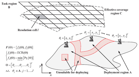
Figure 1.
MFRN deployment problem. The gray areas together form the deployment region.
However, as previously discussed in our earlier work [23], the results yielded by these algorithms are not always satisfactory. This is particularly evident in deployment regions characterized by mathematically complex polygons, including those that exhibit non-connectivity, holes, or concave shapes. This issue quickly drew our attention.
Eventually, inspired by the convex decomposition of complex polygons in computer graphics, we developed a novel method that differs from the prevailing approaches.
1.3. Original Contributions
A novel optimization method for the deployment of MFRNs is proposed to address the challenges posed by complex deployment regions. The key contributions of this paper are as follows:
- (1)
- To effectively tackle the complexities and difficulties encountered when deploying MFRNs in complex regions that may exhibit non-connectivity, holes, or concave shapes, we conduct a comprehensive investigation and expand the problem model.
- (2)
- Utilizing deployment region decomposition and coordinate transformation, we effectively eliminate the constraints imposed by complex deployment regions. Furthermore, by integrating these approaches, we propose a novel algorithm, MOPSO-DT, to optimize MFRN deployment in these challenging environments.
- (3)
- A simulation sample set comprising complex regions of diverse shapes is constructed. The results from comparative experiments indicate that the proposed algorithm considerably outperforms existing methods in terms of efficiency, effectiveness and stability.
1.4. Organization
The subsequent sections of this paper are structured in the following manner. Section 2 elaborates on MFRN deployment in complex regions. In Section 3, we introduce an algorithm specifically designed to facilitate MFRN deployment in these challenging regions. This algorithm employs region decomposition in conjunction with coordinate transformation techniques. Section 4 is dedicated to showcasing the outcomes obtained using the proposed algorithm across various MFRN deployment cases with different deployment regions. Section 5 summarizes the findings.
2. Problem Formulation
The primary focus of this section is to develop a mathematical model for the MFRN deployment problem and analyze the definition and classification of the complex deployment regions where MFRNs are deployed.
2.1. Mathematical Model of the MFRN Deployment Problem
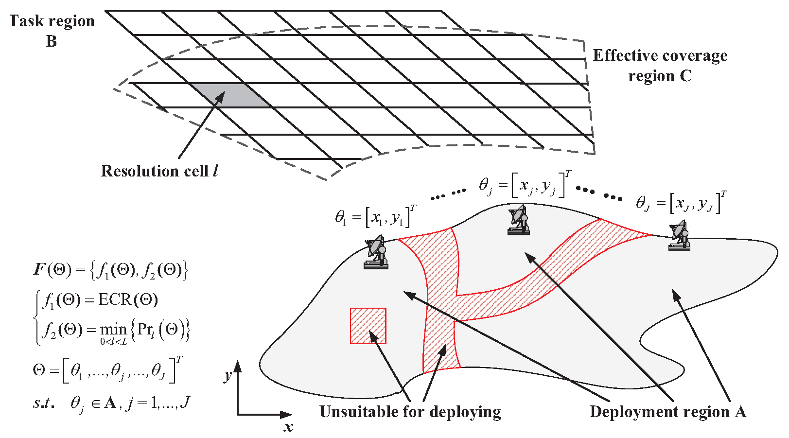
The objective is to enhance surveillance capabilities while simultaneously enhancing suppression jamming effects within the designated task region B, which has been uniformly divided into L resolution cells. The primary constraint addressed in this paper is the requirement that the J nodes of the MFRN are situated within the irregularly defined deployment region designated as A, as shown in Figure 1.
Regarding the optimization objectives, as described in our previous work [22,23], we established optimization objectives for both the surveillance task and the interference suppression task, i.e., the effective detection coverage rate (ECR) and the minimum power density (), respectively. The ECR can be expressed as
where denotes the area of this region and represents the deployment scheme, that is, the precise locations of the J nodes. denotes the l-th effective coverage cell, where in the detection probability exceeds the predefined detection probability threshold .
Let the position of the j-th node be represented by the vector , where and are the Cartesian coordinates of the j-th node. Furthermore, we assume that the MFRN satisfies the following three conditions [19]:
- (i)
- A monopulse square-law detector is employed;
- (ii)
- There exist transceiver channels between each node, and these channels are orthogonal to one another;
- (iii)
- The detected target adheres to the Swerling-I model.
Then, can be expressed as
where represents the Marcum Q function [24]. denotes the total SNR of the l-th resolution cell, and is the detection threshold. Among these factors, the false alarm probability fixes , leaving only to determine . Furthermore, when the performance of each MFRN node is fixed, the detectability factor and the maximum detection range are maintained at constant levels. Therefore, is determined by the distance between the i-th node and the l-th resolution cell, and the distance between the j-th node and the l-th resolution cell, which are represented by and , respectively. Since the positions of all resolution cells are fixed, and are determined by the positions of the J nodes.
The formula for electromagnetic wave propagation in open space indicates that the minimum jamming power density can be expressed as
where is the jammer transmitting power of the j-th node, is the transmitting antenna gain of the j-th node, and is the jamming power density of the l-th resolution cell. It should be noted that the above formula remains valid in all instances, irrespective of the heterogeneity or homogeneity of the nodes within the system.
Given these considerations, the MFRN deployment problem can be expressed as
where is the transpose operation and is the two-dimensional field of real numbers.
It is evident that the primary challenge in this problem lies in addressing the constraints , specifically in modeling the deployment region A.
2.2. Deployment Region Modeling and Analysis
In engineering practice, the deployment region A can be simplified to a polygon, whose boundary consists of straight lines rather than curves. From a mathematical perspective, a of the deployment region is defined as an undirected line segment on the plane of the deployment region, with one side representing the deployment region and the other representing the undeployable region. Moreover, the vertices of the deployment region are defined as the intersections of its sides, as illustrated in Figure 2.
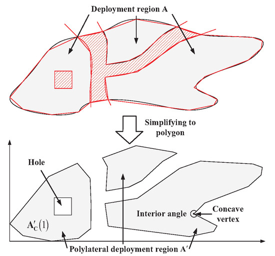
Figure 2.
Polygonal deployment region.
It would be highly preferable for the deployment region A to be represented as a rectangle or, at the very least, a convex polygon (for instance, a triangle, hexagon, or octagon). Mathematically, a convex polygon can be defined as a polygon in which extending any side results in a straight line, with all remaining sides located on the same side of that line.
Nevertheless, as observed in Figure 2, the polygonal deployment region frequently fails to satisfy the definition of a convex polygon, which manifests in three significant ways: (1) It is non-connected. In other words, there exist at least two subregions that are not adjacent to one another. (2) It contains holes. In other words, at least one small polygon in the deployment region does not belong to it. (3) It features concave vertices. In other words, at least one vertex exhibits an interior angle greater than 180 degrees.
For simplicity, this paper refers to a polygonal deployment region exhibiting at least one of three characteristics—it is non-connected, contains holes, or has concave vertices—as a complex deployment region. Conversely, a deployment region that satisfies the definition of a convex polygon is referred to as a convex polygonal deployment region.
3. Deployment Method and Algorithm
The primary objective of this section is to present an algorithm for MFRN deployment in complex deployment regions, utilizing the MOPSO architecture. Section 3.1 proposes a method for decomposing the complex deployment region into several convex deployment subregions, while Section 3.2 focuses on processing convex polygons based on coordinate transformation. Building on this, Section 3.3 provides a comprehensive description of the algorithm for MFRN deployment in complex deployment regions. Section 3.4 introduces two existing algorithms that are employed for comparison with the algorithm proposed in this paper.
3.1. Deployment Region Decomposition
To simplify the complex deployment region into a series of convex deployment subregions, this section proposes a decomposition method based on convex decomposition, as utilized in the field of computer graphics. It sequentially processes non-connected deployment regions, deployment regions with holes, and deployment regions with concave vertices.
3.1.1. Non-Connected Deployment Regions
The processing of the non-connected deployment region, , was the subject of a detailed discussion in our previous work [23]. Specifically, it is divided into a series of connected subregions, , based on their connectivity.
3.1.2. Deployment Regions with Holes
In the framework of a deployment region characterized by holes, , once a vertex on the internal boundary (i.e., the juncture of the deployment region and the hole) is identified, two rays can be drawn from this vertex toward two other vertices of the deployment region, ensuring that these rays do not intersect any other holes. This procedure allows for the division of the region into several subregions that do not contain holes, . The relevant literature has established that a set of such rays invariably exists within a two-dimensional polygon [25].
3.1.3. Deployment Regions with Concave Vertices
The results of studies in the field of computer graphics have demonstrated that a connected and hole-free concave deployment region, , can be divided into a finite number of non-overlapping triangles through convex decomposition, with a complexity of , where n represents the number of vertices of the polygon [26]. These triangles can subsequently be combined to form a series of convex deployment regions, .
3.1.4. Binary Coding for Subregions
As previously stated, a complex deployment region can be decomposed into convex subregions, through the process of convex decomposition. This can be expressed as
where is the k-th convex deployment subregion in the j-th hole-free subregion of the i-th connected subregion. If the deployment region encompasses only one connected subregion or only one hole-free subregion, then i and j can be omitted, respectively. For brevity, the indices i and j are often omitted in the following descriptions.
In addition, a set of binary variables, , is employed to encode the convex deployment subregions. Consequently, any complex deployment region can be represented by a pair of unconstrained continuous variables and binary variables, . Given the use of binary coding, satisfies
where represents the ceiling operator. In this step, an arbitrarily shaped polygonal deployment region is divided into a series of convex subregions. Each is assigned a sequence of binary numbers corresponding to binary variables.
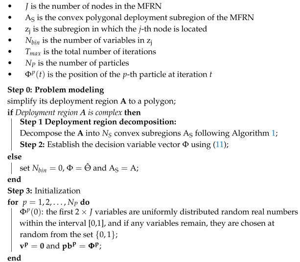
The overall algorithm for region decomposition is presented in Algorithm 1.
| Algorithm 1: Deployment Region Decomposition Algorithm |
 |
3.2. Coordinate Transformation
It is evident that any given point within the designated deployment region must be included in exactly one of the convex subregions, , and not in any others. Given that is a convex polygon, the relative position of an arbitrary point within can be described by a set of normalized continuous variables . In this paper, the aforementioned correspondence is referred to as a coordinate transformation. Without loss of generality, this paper assumes that the coordinate transformation is executed in the following order: the x direction, followed by the y direction. The coordinate transformation can then be defined a
where represents the Euclidean distance, and and denote the upper and lower bounds of in the x direction, respectively. Furthermore, and represent the upper and lower bounds of in the y direction when the value of the x direction is . It is worth noting that the upper and lower bounds are determined by the shape of the convex deployment region (or the subregion in which the coordinate transformation is performed). It is evident that for any two-dimensional convex deployment region, the upper and lower bounds are unique.
Further, the MFRN deployment problem in complex deployment regions can be rephrased as
where denotes the binary number representing the j-th convex deployment subregion and represents the set of all . Meanwhile, represents the n-dimensional field of integer numbers.
The deployment problem is transformed from a constrained multi-objective optimization problem (i.e., Equation (6)) into an unconstrained multi-objective optimization problem (i.e., Equation (10)), despite the incorporation of binary variables.
Equation (10) incorporates both continuous and binary variables. For convenience, all of these decision variables, denoted as , are uniformly represented as
where represents the n-th decision variable.
3.3. Deployment Algorithm for MFRNs in Complex Deployment Regions
Aligning with the approach used in our previous work [23], the deployment algorithm for MFRNs in complex deployment regions was similarly developed based on the MOPSO architectural framework. In other words, the solution process of this algorithm can be described as dispersing a swarm of particles in the feasible domain of (i.e., the deployment region). This algorithm facilitates the exploration of the domain by the particles, influenced by a combination of the inertia factor, the cognitive factor (i.e., the optimal solution identified by each individual particle ), and the social factor (i.e., the optimal solution identified by the entire swarm ). Concurrently, the algorithm stores the and outputs it upon satisfying the termination condition. The motion velocity of the p-th particle at the t-th iteration can be expressed as
where is the velocity vector of the p-th particle, and c, w, and r are the acceleration constant, inertia weight, and a random number that adheres to a uniform distribution on the interval [0,1], respectively.
Correspondingly, the particle position update formula can be expressed as
where represents the of the p-th particle; , , and refer to the n-th variables in their respective vectors; and denotes the inversion operator. , , and are three independent random numbers that follow a uniform distribution on the interval (0, 1). and are the crossover probability and mutation probability, respectively.
The overall deployment algorithm is illustrated in Algorithm 2 [27,28]. Given that this deployment algorithm primarily revolves around deployment region decomposition and coordinate transformation, it is termed MOPSO-DT in this paper.
| Algorithm 2: MFRN Deployment Algorithm in Complex Regions |
 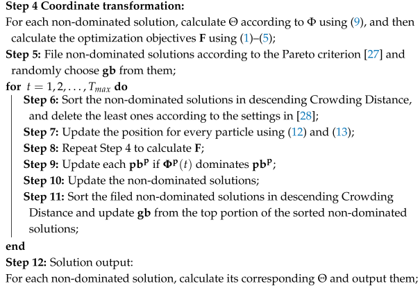 |
3.4. Comparison Algorithms
In order to evaluate the effectiveness of the proposed algorithm, a comparison is required. This section describes two existing MOPSO-based deployment algorithms used for comparison with the algorithm proposed in this paper, MOPSO-DT.
3.4.1. MOPSO-Based Deployment Algorithm with Penalty Function (MOPSO-PF)
This MOPSO-based algorithm employs the penalty function principle, which facilitates the transformation of constraints into an integral component of the optimization objectives [29]. Therefore, this MOPSO-based deployment algorithm with a penalty function is referred to as MOPSO-PF in this paper. When addressing the deployment problem (i.e., Equation (6)) using MOPSO-PF, the corresponding problem that needs to be solved can be expressed as
where represents the optimization objectives with a penalty function, is the extended deployment scheme, and is the minimum external rectangle of the deployment region A. is the penalty function, which consists of one constant term, , and one adaptive term, .
3.4.2. MOPSO-Based Deployment Algorithm with Stochastic Ranking (MOPSO-SR)
The MOPSO-based algorithm employs the stochastic ranking principle, which addresses constrained multi-objective problems by altering the solution sorting strategy [30]. Therefore, this MOPSO-based deployment algorithm with stochastic ranking is referred to as MOPSO-SR in this paper. When solving the deployment problem (i.e., Equation (6)) using MOPSO-SR, the corresponding problem to be solved can be expressed as
The revised criteria for comparing the solutions are as follows: (1) when both solutions are feasible, the Pareto criterion is employed [27]; (2) when one solution is feasible while the other is not, the feasible solution is considered superior; and (3) when neither solution is feasible, the quality of each solution, along with the extent of constraint violation, is combined to make a judgment. Employing this ordering method facilitates the gradual enhancement of particle feasibility.
4. Numerical Study Results and Discussion
This section discusses the performance of the three algorithms introduced in Section 3. It is essential to note that, despite the varying numbers of decision variables (MOPSO-DT: , MOPSO-PF and MOPSO-SR: ) and the apparent distinctions in the models they directly address (for MOPSO-DT: Equation (10); for MOPSO-PF: Equation (14); and for MOPSO-SR: Equation (15)), the underlying physical meanings of these problems remain consistent, and their complexities are comparable.
4.1. Simulation Model and Parameter Settings
In this paper, an MFRN with J nodes is required to simultaneously monitor and jam the task region B, which measures 300 km × 300 km. Furthermore, B is uniformly subdivided into 900 resolution cells, each of which measures 10 km × 10 km. The task region and resolution cells are illustrated schematically in Figure 3a. The entire rectangular area is designated as the task region B, where each grid cell represents a resolution cell.
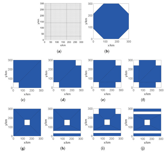
Figure 3.
Locations of the task region and the deployment regions for each case. (a) Task region of the MFRN. (b) Deployment regions for Cases 1–4. (c–j) Deployment regions for Cases 5–12. Within each subfigure, the section depicted in blue represents the deployment region, while the black dotted line demarcates the boundary separating the convex subregions resulting from the region decomposition process.
The deployment region A overlaps with the task region with additional constraints. This paper presents 12 distinct simulation cases based on the number of nodes, constraints, and the specific geometries associated with these constraints. The simulation cases encompass all types of complex deployment regions, including non-connected regions, those with holes, or those with concave shapes.
The 12 cases have nine different geometric shapes, whose sketches are shown in Figure 3b–j. The specific features, along with the number of nodes and constraints for each case, are presented in Table 1. Furthermore, Figure 3 depicts the results of the decomposition of the deployment region, as identified by Algorithm 1, which is indicated by a black dotted line.

Table 1.
Features and key parameters of the deployment regions for the 12 cases.
It should be noted that the proposed method maintains theoretical validity regardless of the complexity and fragmentation of the deployment region, given the framework assumption of this paper, that is, that the deployment region is a two-dimensional polygonal region. This assertion is supported by research in the field of computer graphics [25], which shows that any two-dimensional polygon can be decomposed into multiple convex polygons using convex partitioning methods.
Moreover, all nodes in the MFRN have equivalent performance. For each node, the transmission power is set to 3 kW, the antenna transmit-receive gain is set to 50 dB, the target RCS is set to 0.1 m2, the signal wavelength is 0.3 m, and the signal bandwidth is 15 MHz. Additionally, the detection factor is set to , and the false alarm rate is set to . According to the radar formula [24], the maximum detection range for achieving typical targets is km. The jamming function is characterized by a jammer transmitting power of W and a jamming transmitting antenna gain of .
In terms of the public parameters of the three algorithms, , and the acceleration constants are . The inertia factor w decreases with each iteration, where w of the t-th iteration is × t + 0.4. For MOPSO-PF, the constant penalty function is set to
, and the adaptive term,
, is defined as the sum of the Euclidean
distances from each node outside the deployment region to the boundary of the nearest
deployment region. For MOPSO-DT, the crossover probability
and the mutation
probability
Regarding the calculation costs, the maximum number of iterations, , for the three algorithms is consistent, each set to 500 iterations. Furthermore, all three algorithms perform 100 Monte Carlo experiments.
The MFRN deployment problem addressed in this paper is formulated as a multi-objective optimization problem. To quantitatively measure the quality of the solutions to this problem, this paper introduces the hypervolume (HV) as a metric of solution quality. The HV is a performance index commonly employed in the field of multi-objective optimization and is based on the Lebesgue measure [31]. A higher HV indicates a superior quality of a solution or a set of solutions. The reference point of the HV is set to (0, 0) in this paper.
4.2. Results Analysis
The results of the simulation are analyzed below in terms of algorithm efficiency, effectiveness, and stability.
4.2.1. Algorithm Efficiency
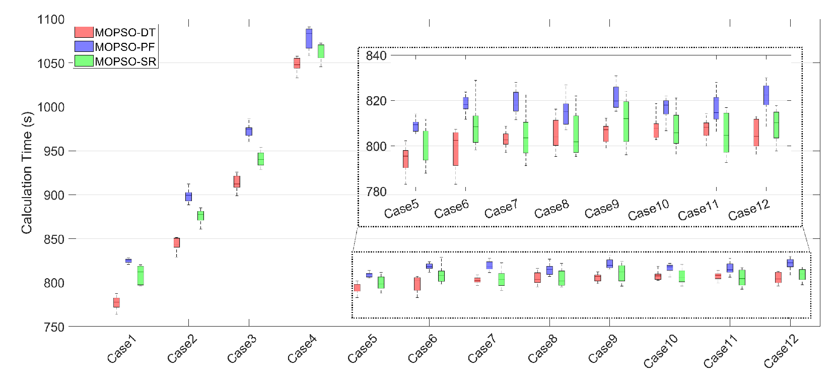
All simulations presented in this paper were conducted on the same computing device, which was equipped with a 3.5 GHz CPU and 3600 MHz of RAM. Figure 4 presents the required calculation time for the completion of each case, as illustrated in the corresponding box plots. Based on Figure 4, the following observations can be made:

Figure 4.
The box plots of the calculation time for the completion of each of the 12 cases. The enlarged box plots for Cases 5–12 are presented in a dotted-frame box in the upper-right corner. All simulations presented in this paper were conducted on the same computing device, which was equipped with a 3.5 GHz CPU and 3600 MHz of RAM.
- (1)
- The calculation time increased from Cases 1–4, indicating the impact of the problem scale (i.e., the number of nodes J) on the performance of the algorithms. It is important to note that as the problem scale increased, the rise in calculation costs was not solely attributed to the process of calculating the subsequent generation of solution values during the algorithmic iterations. Rather, it also resulted from the expansion of the calculations associated with the objective function. Additionally, the times required to solve Case 1 and Cases 5–12 were approximately the same, indicating that the constraints discussed in this paper did not significantly impact the efficiency of the algorithms.
- (2)
- The results indicate that MOPSO-DT demonstrated superior efficiency compared to existing algorithms, as evidenced by the relatively lower-positioned red box plots observed in each case. Concurrently, MOPSO-SR required less computation time compared to MOPSO-PF. This conclusion is reasonable, given that MOPSO-SR does not entail the calculation of the penalty function.
These findings provide evidence of the superiority of the proposed deployment algorithm in terms of algorithm efficiency.
4.2.2. Algorithm Effectiveness
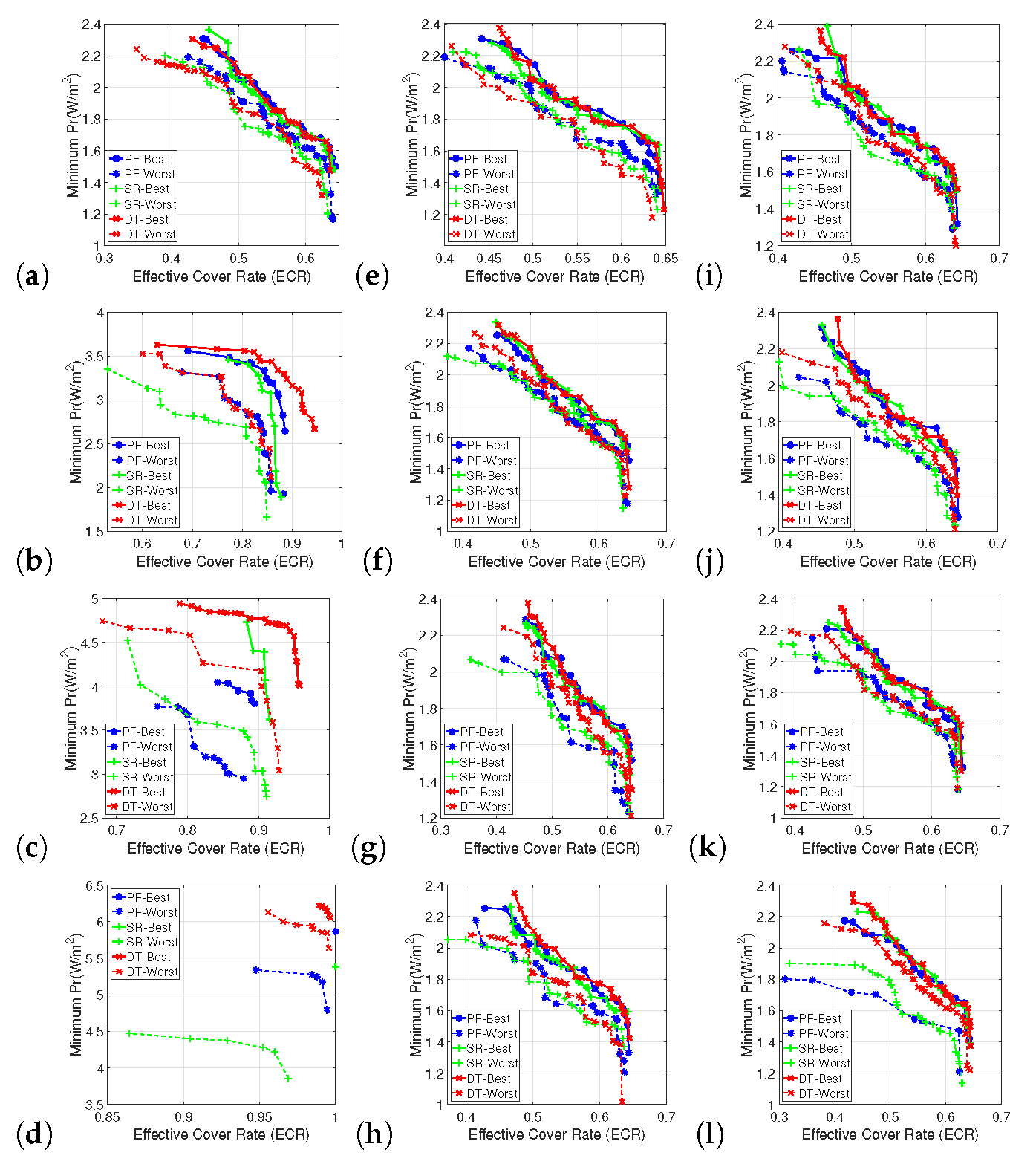
The subfigures in Figure 5 present the output solutions yielded by the three algorithms when addressing the 12 cases. Given the considerable volume of output solutions, the figure exclusively depicts those that are optimal according to the Pareto criterion, identified by a thicker solid line. Additionally, it depicts the least optimal solutions, identified by a thinner dashed line. Table 2 presents the mean and standard deviation (SD) of the HV values of the final output solutions obtained with the three algorithms. Based on the data presented in Figure 5 and Table 2, the following observations can be made:
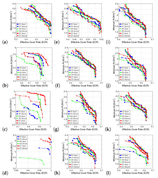
Figure 5.
The optimal solutions (marked by the thicker solid line) and the least optimal solutions (marked by the thinner dashed line) under the Pareto criterion, obtained with the three algorithms. The red curve represents the results obtained with MOPSO-DT, the blue curve represents the results obtained with MOPSO-PF, and the green curve represents the results obtained with MOPSO-SR. (a–l) Cases 1–12.
Table 2.
The statistical data for the HV values of the solutions obtained with each algorithm when solving the 12 cases. The first number in each cell denotes the mean HV of the solutions obtained with the algorithm in the corresponding column when solving the case in the corresponding row. The number following the symbol ± represents the standard deviation (SD) of these solutions. The number in the latter bracket represents the ranking among the three algorithms.
- (1)
- There was a significant conflict between the optimization objectives, ECR and , as outlined in this paper, meaning that optimizing one objective typically occurred at the expense of the other.
- (2)
- Despite the apparent presence of additional constraints in Case 11 compared to Case 12, the non-connected subregions posed a more significant challenge for the algorithm than the concave vertices. This observation is supported by the simulation results, which indicate that the existing algorithms were less effective in solving Case 12.
- (3)
- Given that the deployment region for Cases 1–4 was convex (as illustrated in Figure 3b), the region decomposition component proposed in this paper was inapplicable, leaving only the coordinate transformation component to be effective. As evidenced by the data in Table 2, our method still demonstrated an advantage, albeit with a reduced magnitude compared to other cases where both region decomposition and coordinate transformation were effective. This observation highlights the effectiveness of the coordinate transformation approach. Figure 5a–d also corroborate this conclusion.
- (4)
- As evidenced by the data presented in Table 2, in most cases, MOPSO-PF outperformed MOPSO-SR, with the exception of two instances in which MOPSO-SR demonstrated a slight advantage. This finding supports the conclusion that MOPSO-PF has an advantage over MOPSO-SR in terms of algorithm efficiency.
- (5)
- In all 12 cases, the mean value of the HV of the solutions obtained using MOPSO-DT exceeded that of the other two algorithms. This advantage was statistically significant at the 5% level in all cases, except for case 1.
These findings provide evidence of the superiority of the proposed deployment algorithm in terms of algorithm effectiveness.
4.2.3. Algorithm Stability
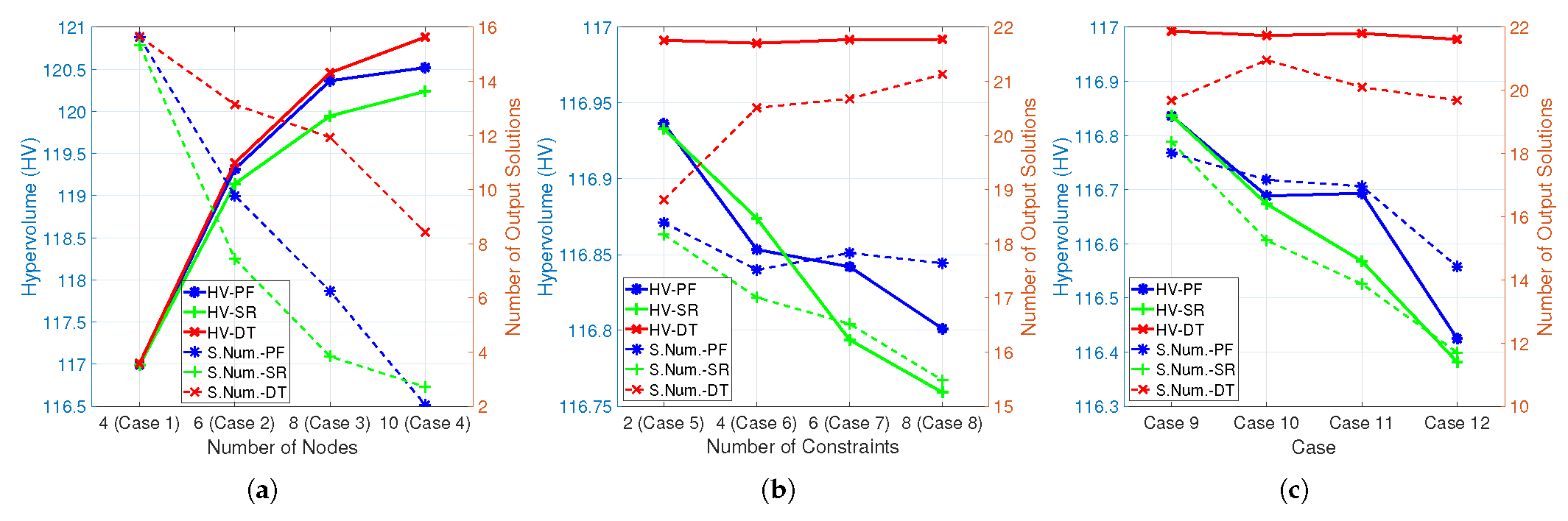
The mean value of the HV and the number of solutions obtained with the three algorithms is plotted in three groups within the subplots of Figure 6.
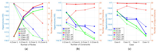
Figure 6.
The mean value of the HV and the number of solutions in each case. The HV is marked by a thicker solid line, while the mean number of solutions is marked by a thinner dotted line. The red curve represents the results obtained with MOPSO-DT, the blue curve represents the results obtained with MOPSO-PF, and the green curve represents the results obtained with MOPSO-SR. (a) Cases 1–4. (b) Cases 5–8. (c) Cases 9–12.
The stability of the algorithm is analyzed from the following three aspects: sensitivity to problem scale, sensitivity to problem complexity, and consistency of solution quality.
(1) Sensitivity to problem scale: As illustrated in Figure 6a, the quality of the solutions (measured by HV) obtained with the three algorithms improves as the problem scale (i.e., the number of nodes) increases. This is due to the fact that an increased number of nodes results in a greater number of transceiver channels, which, in turn, leads to an improvement in the overall detection and interference performance of the MFRN. However, this improvement in solution quality among the three algorithms is not consistent as the scale expands. As the scale of the problem expands, MOPSO-DT shows a more significant advantage over the existing algorithms. The same observations can be made with regard to Figure 5a–d.
Concurrently, it is evident that while the mean number of solutions obtained with the three algorithms declines as the problem scale expands, MOPSO-DT exhibits the most gradual decline.
Therefore, it can be concluded that MOPSO-DT exhibits superior stability as problem complexity increases.
(2) Sensitivity to problem complexity: As illustrated in Figure 6b,c, as the complexity of the problem increases, the quality of the solutions obtained with the two existing algorithms is significantly reduced, while the number of solutions also decreases. In contrast, MOPSO-DT demonstrates no substantial decline in either of these aspects. Thus, it can be concluded that MOPSO-DT exhibits superior stability when faced with increasing problem complexity. A similar conclusion can be drawn by examining Figure 5e–h and Figure 5i–l.
It should be noted that the three algorithms under discussion in this paper are all based on the MOPSO architecture. It is known that MOPSO has proven asymptotic convergence properties [32], which means that the advantage of MOPSO-DT in terms of stability, compared to existing algorithms, can be extended to more complex scenarios, particularly those characterized by more fragmented deployment regions and, consequently, a larger .
(3) Consistency of solution quality: In Table 2, MOPSO-DT has the lowest standard deviation across 100 Monte Carlo experiments, indicating that its solutions exhibit greater consistency in solution quality.
By considering the above three points, it can be concluded that MOPSO-DT generally demonstrates superior stability compared to the two existing algorithms.
5. Conclusions
In this paper, a region decomposition approach is proposed to effectively address the challenges posed by complex deployment regions. By addressing deployment regions exhibiting non-connectivity, holes, and concave shapes in a sequential manner, it is possible to transform an arbitrary complex polygonal deployment region into a series of convex subregions. For convex deployment regions or subregions, we propose a coordinate transformation approach based on linear mapping that can eliminate the constraints introduced by the shape of the convex region. The above approaches are combined to create a novel MOPSO-based decomposition and transformation (MOPSO-DT) method, for which a series of numerical simulation experiments have demonstrated its advantages in terms of efficiency, effectiveness, and stability when optimizing MFRN deployment in complex regions.
The elimination of constraints imposed by the deployment region, coupled with enhanced deployment efficiency, renders this method an effective means of reducing the complexity of MFRN or any multi-static radar deployment within complex regions. Furthermore, this approach offers insights that can be applied to related fields, such as sensor network deployment.
In the future, our research will continue in two distinct but complementary directions. The initial objective will be to extend the region decomposition method proposed in this paper to three-dimensional space and explore the adaptive decomposition technique. Equally importantly, it will be beneficial to investigate the extension of the mapping model of the coordinate transformation approach and the dynamic re-mapping method. In order to align the proposed method with real-world practice, it is imperative to apply the proposed methods to more real-world complexities, such as dynamic environments and highly fragmented deployment regions.
Author Contributions
Conceptualization, X.L. and T.Z.; methodology, Y.H., Z.Z., and T.Z.; software and validation, Y.H. and Z.Z.; writing—original draft preparation, Y.H. and X.X.; writing—review and editing, X.X., X.L., and T.Z.; supervision, X.Y. All authors have read and agreed to the published version of the manuscript.
Funding
This work was supported by the Qianyuan Laboratory.
Data Availability Statement
Data are contained within the article. All data in this paper are generated through simulation, and the details are presented in Section 4.
Acknowledgments
We would like to extend our appreciation to the editors and reviewers for their insightful comments, which helped improve the quality of this manuscript. Additionally, the editorial team’s efforts in English editing, proofreading, and formatting the manuscript are greatly appreciated, as these actions have enhanced its readability.
Conflicts of Interest
The authors declare no conflicts of interest. The funder had no role in the design of the study; in the collection, analyses, or interpretation of data; in the writing of the manuscript; or in the decision to publish the results.
Abbreviations
The following abbreviations are used in this manuscript:
| MFRN | Multi-functional radar network |
| MOPSO | Multi-objective particle swarm optimization |
| MIMO | Multiple-input multiple-output |
| GDOP | Geometric dilution of precision |
| CRLB | Cramer–Rao lower bound |
| SNR | Signal-to-noise ratio |
| PSO | Particle swarm optimization |
| ECR | Effective coverage rate |
| Pr | Power density |
| MOPSO-DT | MOPSO-based Deployment Algorithm with Decomposition and Transformation |
| MOPSO-PF | MOPSO-based Deployment Algorithm with Penalty Function |
| MOPSO-SR | MOPSO-based Deployment Algorithm with Stochastic Ranking |
| HV | Hypervolume |
References
- Javadi, S.H.; Farina, A. Radar networks: A review of features and challenges. Inf. Fusion 2020, 61, 48–55. [Google Scholar] [CrossRef]
- Yan, H.; Zhang, S.; Lu, X.; Yang, J.; Duan, L.; Tan, K.; Gu, H. A Waveform Design for Integrated Radar and Jamming Based on Smart Modulation and Complementary Coding. Remote Sens. 2024, 16, 2725. [Google Scholar] [CrossRef]
- Kilani, M.B.; Gagnon, G.; Gagnon, F. Multistatic radar placement optimization for cooperative radar-communication systems. IEEE Commun. Lett. 2018, 22, 1576–1579. [Google Scholar] [CrossRef]
- Liu, H.; Li, Y.; Cheng, W.; Dong, L.; Yan, B. Sensing-Efficient Transmit Beamforming for ISAC with MIMO Radar and MU-MIMO Communication. Remote Sens. 2024, 16, 3028. [Google Scholar] [CrossRef]
- Wang, Y.; Zhou, T.; Yi, W. Geometric optimization of distributed MIMO radar system for accurate localization in multiple key subareas. Signal Process. 2022, 201, 108689. [Google Scholar] [CrossRef]
- Yan, J.; Zhang, T.; Ma, L.; Pu, W.; Liu, H. Deployment Optimization for Integrated Search and Tracking Tasks in Netted Radar System Based on Pareto Theory. IEEE Trans. Aerosp. Electron. Syst. 2024, 60, 3664–3672. [Google Scholar] [CrossRef]
- Chen, W.J.; Narayanan, R.M. Antenna placement for minimizing target localization error in UWB MIMO noise radar. IEEE Antennas Wirel. Propag. Lett. 2011, 10, 135–138. [Google Scholar] [CrossRef]
- Gong, X.; Zhang, J.; Cochran, D.; Xing, K. Optimal placement for barrier coverage in bistatic radar sensor networks. IEEE/ACM Trans. Netw. 2014, 24, 259–271. [Google Scholar] [CrossRef]
- Sun, B.; Chen, H.; Yang, D.; Li, X. Antenna selection and placement analysis of MIMO radar networks for target localization. Int. J. Distrib. Sens. Netw. 2014, 10, 769404. [Google Scholar] [CrossRef]
- Sadeghi, M.; Behnia, F.; Amiri, R. Optimal geometry analysis for TDOA-based localization under communication constraints. IEEE Trans. Aerosp. Electron. Syst. 2021, 57, 3096–3106. [Google Scholar] [CrossRef]
- Niu, C.; Zhang, Y.; Guo, J. Pareto optimal layout of multistatic radar. Signal Process. 2018, 142, 152–156. [Google Scholar] [CrossRef]
- Radmard, M.; Chitgarha, M.M.; Majd, M.N.; Nayebi, M.M. Antenna placement and power allocation optimization in MIMO detection. IEEE Trans. Aerosp. Electron. Syst. 2014, 50, 1468–1478. [Google Scholar] [CrossRef]
- Shi, W.; He, Q.; Sun, L. Transmit antenna placement based on graph theory for MIMO radar detection. IEEE Trans. Signal Process. 2022, 70, 3993–4005. [Google Scholar] [CrossRef]
- Liang, J.; Huan, M.; Deng, X.; Bao, T.; Wang, G. Optimal transmitter and receiver placement for localizing 2D interested-region target with constrained sensor regions. Signal Process. 2021, 183, 108032. [Google Scholar] [CrossRef]
- Xie, R.; Luo, K.; Jiang, T. Joint coverage and localization driven receiver placement in distributed passive radar. IEEE Trans. Geosci. Remote Sens. 2020, 59, 1094–1105. [Google Scholar] [CrossRef]
- Lackpour, A.; Proska, K. GOMERS: Genetic optimization of a multistatic extended radar system. In Proceedings of the 2016 IEEE Radar Conference (RadarConf), Philadelphia, PA, USA, 2–6 May 2016; pp. 1–6. [Google Scholar]
- Zhang, Z.; Li, X.; Zhang, Z.; Wang, M.; Chen, H.; Cui, G. Optimal Placement Method of Netted MIMO Radar Nodes Based on Hybrid Integration for Surveillance Applications. IEEE Trans. Aerosp. Electron. Syst. 2024, 60, 3537–3552. [Google Scholar] [CrossRef]
- Su, Y.; Cheng, T.; He, Z. Collaborative trajectory planning and transmit resource scheduling for multiple target tracking in distributed radar network system with GTAR. Signal Process. 2024, 223, 109550. [Google Scholar] [CrossRef]
- Yang, Y.; Yi, W.; Zhang, T.; Cui, G.; Kong, L.; Yang, X.; Yang, J. Fast optimal antenna placement for distributed MIMO radar with surveillance performance. IEEE Signal Process. Lett. 2015, 22, 1955–1959. [Google Scholar] [CrossRef]
- Yang, Y.; Zhang, T.; Yi, W.; Kong, L.; Li, X.; Wang, B.; Yang, X. Deployment of multistatic radar system using multi-objective particle swarm optimisation. IET Radar Sonar Navig. 2018, 12, 485–493. [Google Scholar] [CrossRef]
- Li, X.; Wang, R.; Liang, G.; Yang, Z. A Multi-Objective Intelligent Optimization Method for Sensor Array Optimization in Distributed SAR-GMTI Radar Systems. Remote Sens. 2024, 16, 3041. [Google Scholar] [CrossRef]
- Zhang, T.; Liang, J.; Yang, Y.; Cui, G.; Kong, L.; Yang, X. Antenna deployment method for multistatic radar under the situation of multiple regions for interference. Signal Process. 2018, 143, 292–297. [Google Scholar] [CrossRef]
- Han, Y.; Li, X.; Zhang, T.; Yang, X. Multi-Static Radar System Deployment Within a Non-Connected Region Utilising Particle Swarm Optimization. Remote Sens. 2024, 16, 4004. [Google Scholar] [CrossRef]
- Richards, M.A. Fundamentals of Radar Signal Processing; Mcgraw-Hill: New York, NY, USA, 2005; Volume 1. [Google Scholar]
- Martini, H.; Soltan, P. On convex partitions of polygonal regions. Discret. Math. 1999, 195, 167–180. [Google Scholar] [CrossRef]
- Narkhede, A.; Manocha, D. Fast polygon triangulation based on seidel’s algorithm. In Graphics Gems V; Elsevier: Amsterdam, The Netherlands, 1995; pp. 394–397. [Google Scholar]
- Miettinen, K. Nonlinear Multiobjective Optimization; Springer Science & Business Media: Berlin/Heidelberg, Germany, 1999; Volume 12. [Google Scholar]
- Raquel, C.R.; Naval, P.C., Jr. An effective use of crowding distance in multiobjective particle swarm optimization. In Proceedings of the 7th Annual Conference on Genetic and Evolutionary Computation, Washington, DC, USA, 25–29 June 2005; pp. 257–264. [Google Scholar]
- Gao, W.F.; Yen, G.G.; Liu, S.Y. A dual-population differential evolution with coevolution for constrained optimization. IEEE Trans. Cybern. 2014, 45, 1108–1121. [Google Scholar] [CrossRef]
- Runarsson, T.P.; Yao, X. Stochastic ranking for constrained evolutionary optimization. IEEE Trans. Evol. Comput. 2000, 4, 284–294. [Google Scholar] [CrossRef]
- Zitzler, E.; Thiele, L.; Laumanns, M.; Fonseca, C.M.; Da Fonseca, V.G. Performance assessment of multiobjective optimizers: An analysis and review. IEEE Trans. Evol. Comput. 2003, 7, 117–132. [Google Scholar] [CrossRef]
- Chakraborty, P.; Das, S.; Roy, G.G.; Abraham, A. On convergence of the multi-objective particle swarm optimizers. Inf. Sci. 2011, 181, 1411–1425. [Google Scholar] [CrossRef]


Disclaimer/Publisher’s Note: The statements, opinions and data contained in all publications are solely those of the individual author(s) and contributor(s) and not of MDPI and/or the editor(s). MDPI and/or the editor(s) disclaim responsibility for any injury to people or property resulting from any ideas, methods, instructions or products referred to in the content. |
© 2025 by the authors. Licensee MDPI, Basel, Switzerland. This article is an open access article distributed under the terms and conditions of the Creative Commons Attribution (CC BY) license (https://creativecommons.org/licenses/by/4.0/).