
Revisiting the 2020 Mw 6.8 Elaziğ, Türkiye Earthquake with Physics-Based 3D Numerical Simulations Constrained by Geodetic and Seismic Observations

 , , , ,
Abstract
1. Introduction
2. Materials and Methods
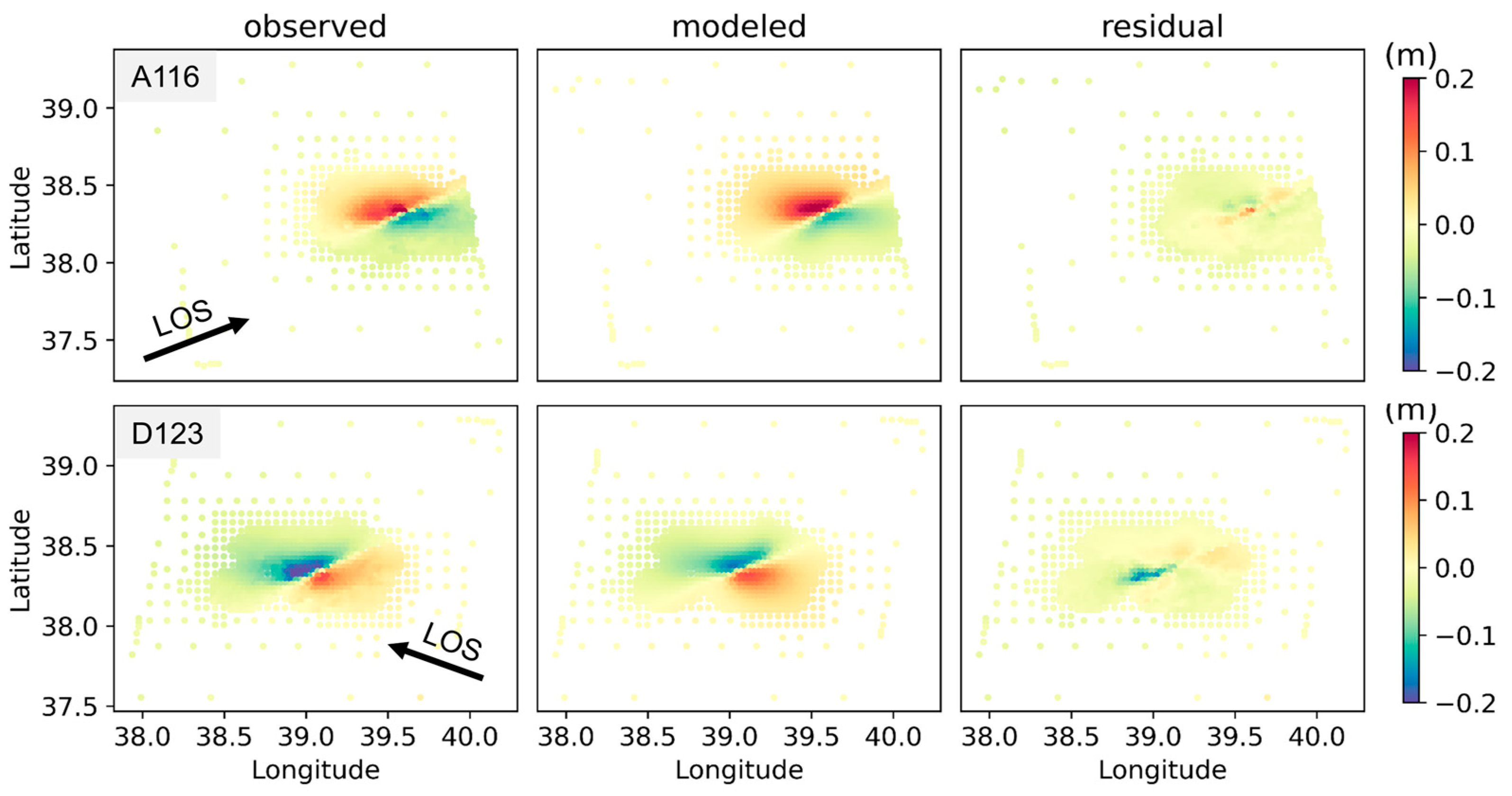
2.1. InSAR and Strong Motion Data
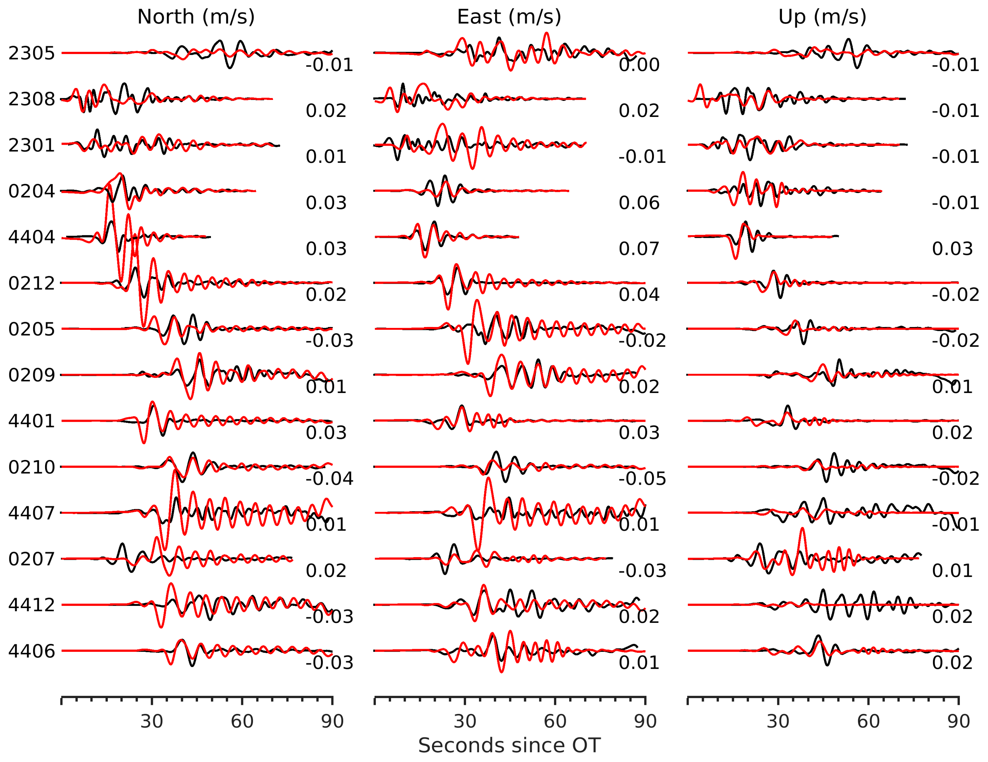
2.2. Kinematic Inversion
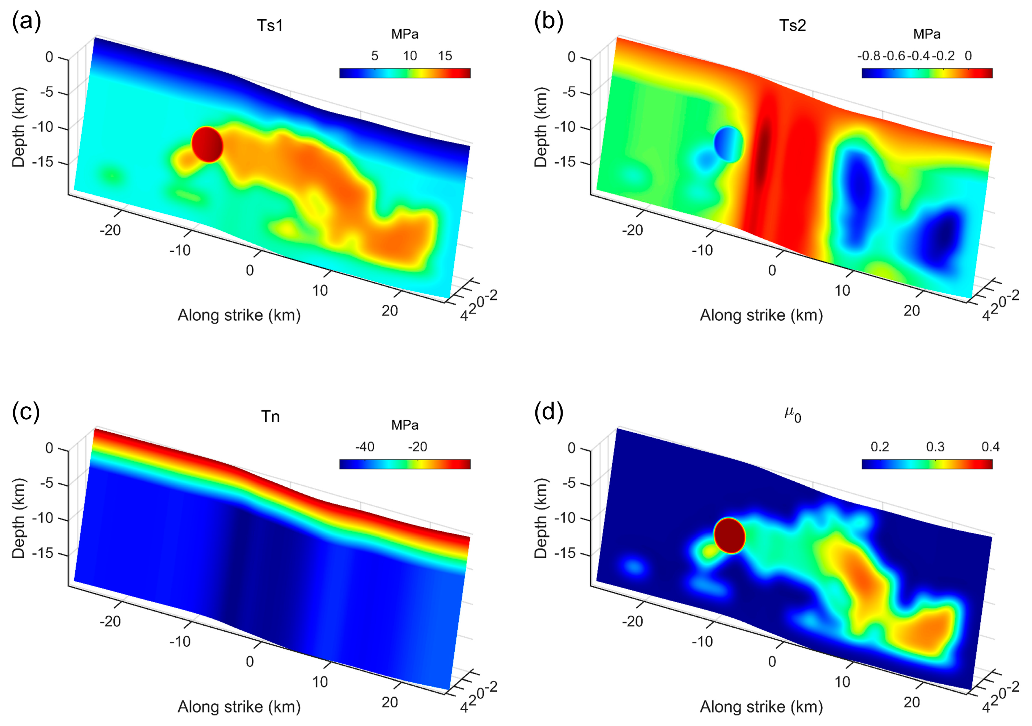
2.3. Dynamic Rupture Simulations
3. Results
3.1. Preferred Kinematic Model
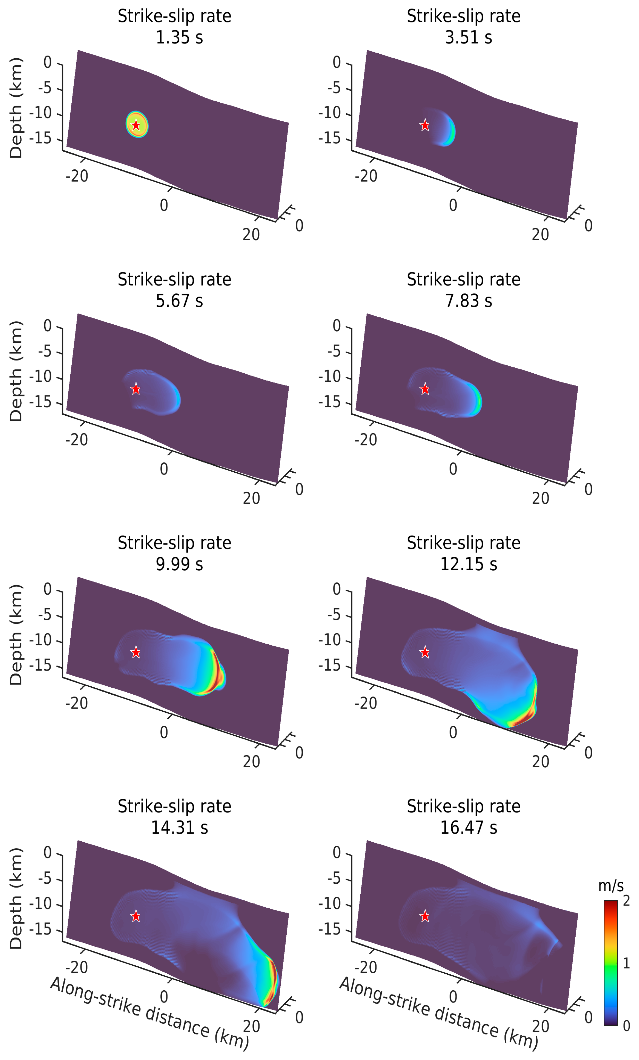
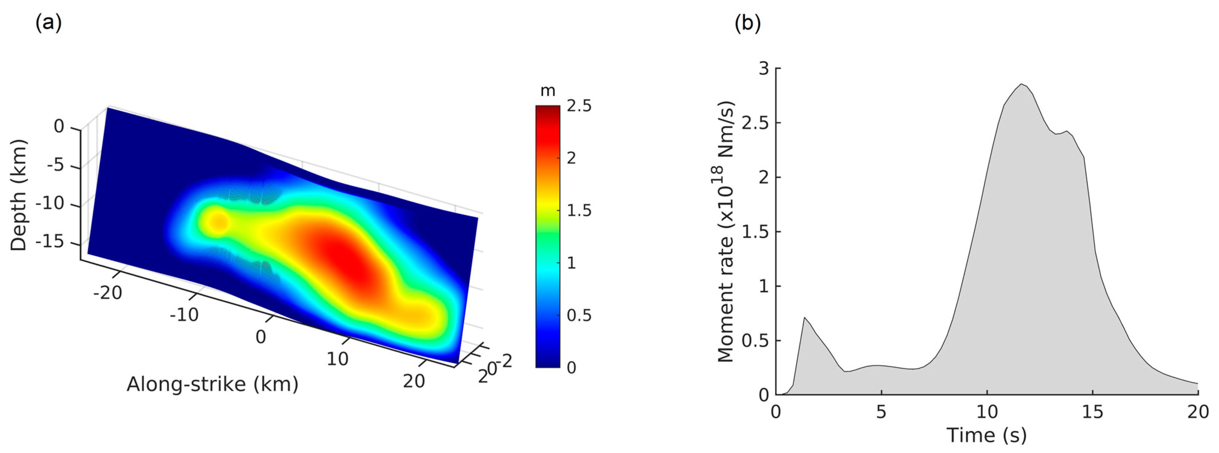
3.2. Dynamic Rupture Model
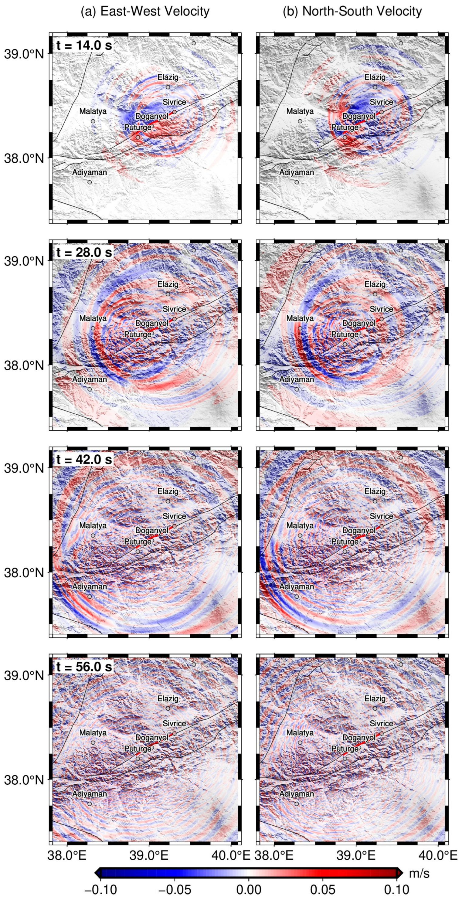
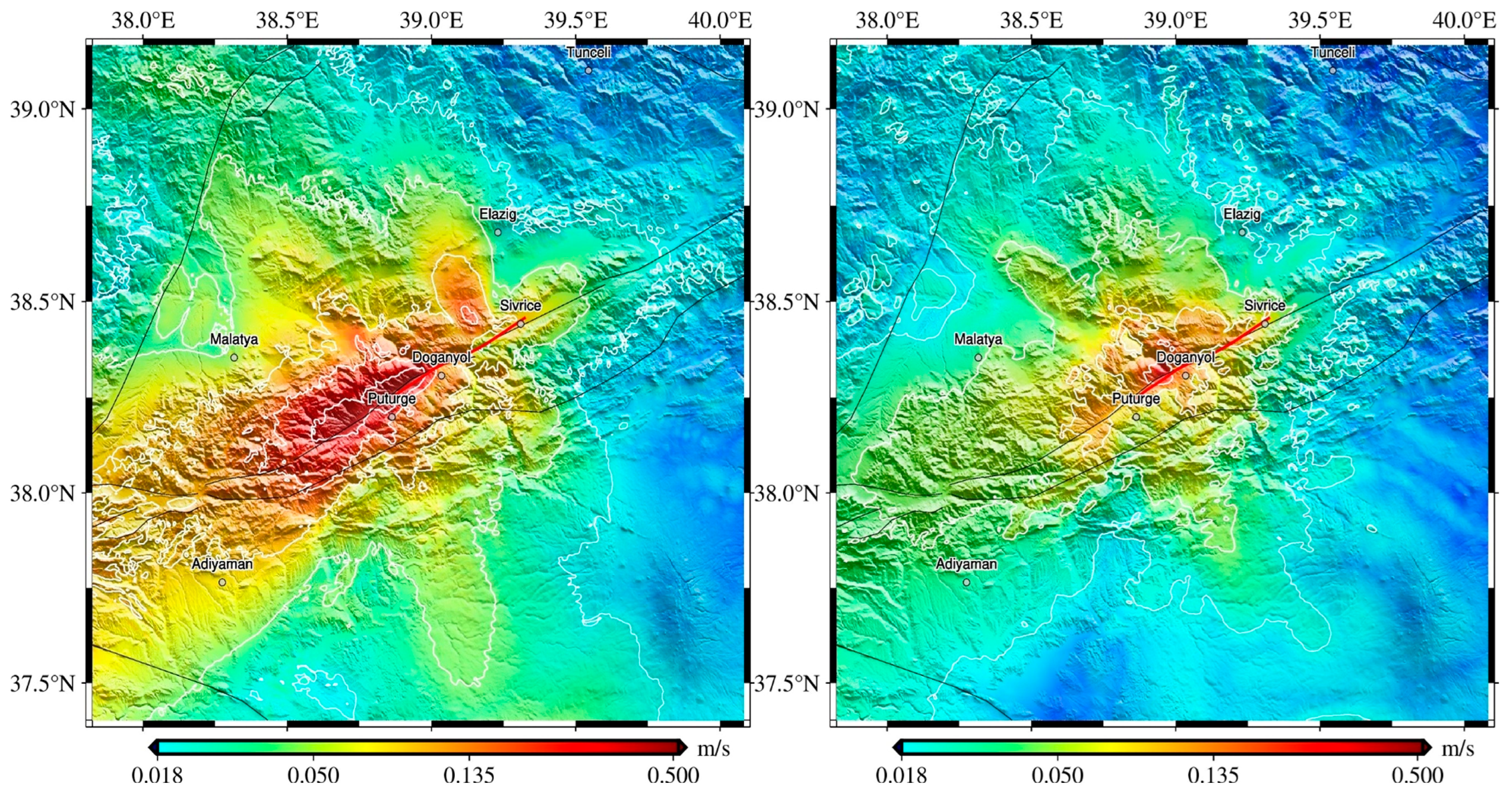
3.3. Simulated Ground Motion
4. Discussion
5. Conclusions
Supplementary Materials
Author Contributions
Funding
Data Availability Statement
Acknowledgments
Conflicts of Interest
References
- Çetin, K.Ö.; Ilgaç, M.; Can, G.; Çakır, E.; Söylemez, B. Sivrice-Elazig-Turkey Earthquake Reconnaissance Report. DesignSafe-CI, 24 January 2020. [Google Scholar] [CrossRef]
- Duman, T.Y.; Emre, Ö. The East Anatolian Fault: Geometry, segmentation and jog characteristics. Geol. Soc. Lond. Spec. Publ. 2013, 372, 495–529. [Google Scholar] [CrossRef]
- Yilmaz, H.; Over, S.; Ozden, S. Kinematics of the East Anatolian Fault Zone between Turkoglu (Kahramanmaras) and Celikhan (Adiyaman), eastern Turkey. Earth Planets Space 2006, 58, 1463–1473. [Google Scholar] [CrossRef]
- Ambraseys, N.N.; Jackson, J.A. Faulting associated with historical and recent earthquakes in the Eastern Mediterranean region. Geophys. J. Int. 1998, 133, 390–406. [Google Scholar] [CrossRef]
- Tan, O.; Taymaz, T. Active tectonics of the Caucasus: Earthquake source mechanisms and rupture histories obtained from inversion of teleseismic body waveforms. In Postcollisional Tectonics and Magmatism in the Mediterranean Region and Asia; Dilek, Y., Pavlides, S., Eds.; Geological Society of America: Boulder, CO, USA, 2006. [Google Scholar]
- Taymaz, T.; Eyidoğan, H.; Jackson, J. Source parameters of large earthquakes in the East Anatolian Fault Zone (Turkey). Geophys. J. Int. 1991, 106, 537–550. [Google Scholar] [CrossRef]
- Taymaz, T.; Ganas, A.; Yolsal-Çevikbilen, S.; Vera, F.; Eken, T.; Erman, C.; Keleş, D.; Kapetanidis, V.; Valkaniotis, S.; Karasante, I.; et al. Source Mechanism and Rupture Process of the 24 January 2020 Mw 6.7 Doğanyol–Sivrice Earthquake obtained from Seismological Waveform Analysis and Space Geodetic Observations on the East Anatolian Fault Zone (Turkey). Tectonophysics 2021, 804, 228745. [Google Scholar] [CrossRef]
- Chen, J.; Liu, C.; Dal Zilio, L.; Cao, J.; Wang, H.; Yang, G.; Göğüş, O.H.; Zhang, H.; Shi, Y. Decoding Stress Patterns of the 2023 Türkiye-Syria Earthquake Doublet. J. Geophys. Res. Solid Earth 2024, 129, e2024JB029213. [Google Scholar] [CrossRef]
- Nocquet, J.-M. Present-day kinematics of the Mediterranean: A comprehensive overview of GPS results. Tectonophysics 2012, 579, 220–242. [Google Scholar] [CrossRef]
- Pousse-Beltran, L.; Nissen, E.; Bergman, E.A.; Cambaz, M.D.; Gaudreau, É.; Karasözen, E.; Tan, F. The 2020 6.8 Elazığ (Turkey) Earthquake Reveals Rupture Behavior of the East Anatolian Fault. Geophys. Res. Lett. 2020, 47, e2020GL088136. [Google Scholar] [CrossRef]
- Melgar, D.; Ganas, A.; Taymaz, T.; Valkaniotis, S.; Crowell, B.W.; Kapetanidis, V.; Tsironi, V.; Yolsal-Çevikbilen, S.; Öcalan, T. Rupture kinematics of 2020 January 24 Mw 6.7 Doğanyol-Sivrice, Turkey earthquake on the East Anatolian Fault Zone imaged by space geodesy. Geophys. J. Int. 2020, 223, 862–874. [Google Scholar] [CrossRef]
- Cheloni, D.; Akinci, A. Source modelling and strong ground motion simulations for the 24 January 2020, Mw 6.8 Elazığ earthquake, Turkey. Geophys. J. Int. 2020, 223, 1054–1068. [Google Scholar] [CrossRef]
- Ragon, T.; Simons, M.; Bletery, Q.; Cavalié, O.; Fielding, E. A Stochastic View of the 2020 Elazığ Mw 6.8 Earthquake (Turkey). Geophys. Res. Lett. 2021, 48, e2020GL090704. [Google Scholar] [CrossRef]
- Konca, A.Ö.; Karabulut, H.; Güvercin, S.E.; Eskiköy, F.; Özarpacı, S.; Özdemir, A.; Floyd, M.; Ergintav, S.; Doğan, U. From Interseismic Deformation with Near-Repeating Earthquakes to Co-Seismic Rupture: A Unified View of the 2020 Mw6.8 Sivrice (Elazığ) Eastern Turkey Earthquake. J. Geophys. Res. Solid Earth 2021, 126, e2021JB021830. [Google Scholar] [CrossRef]
- Lin, X.; Hao, J.; Wang, D.; Chu, R.; Zeng, X.; Xie, J.; Zhang, B.; Bai, Q. Coseismic Slip Distribution of the 24 January 2020 Mw 6.7 Doganyol Earthquake and in Relation to the Foreshock and Aftershock Activities. Seismol. Res. Lett. 2020, 92, 127–139. [Google Scholar] [CrossRef]
- Xu, J.; Liu, C.; Xiong, X. Source Process of the 24 January 2020 Mw 6.7 East Anatolian Fault Zone, Turkey, Earthquake. Seismol. Res. Lett. 2020, 91, 3120–3128. [Google Scholar] [CrossRef]
- Chen, K.; Zhang, Z.; Liang, C.; Xue, C.; Liu, P. Kinematics and Dynamics of the 24 January 2020 M 6.7 Elazig, Turkey Earthquake. Earth Space Sci. 2020, 7, e2020EA001452. [Google Scholar] [CrossRef]
- Tatar, O.; Sözbilir, H.; Koçbulut, F.; Bozkurt, E.; Aksoy, E.; Eski, S.; Özmen, B.; Alan, H.; Metin, Y. Surface deformations of 24 January 2020 Sivrice (Elazığ)–Doğanyol (Malatya) earthquake (Mw = 6.8) along the Pütürge segment of the East Anatolian Fault Zone and its comparison with Turkey’s 100-year-surface ruptures. Mediterr. Geosci. Rev. 2020, 2, 385–410. [Google Scholar] [CrossRef]
- Zhang, Z.; Zhang, W.; Chen, X. Dynamic Rupture Simulations of the 2008 Mw 7.9 Wenchuan Earthquake by the Curved Grid Finite-Difference Method. J. Geophys. Res. Solid Earth 2019, 124, 10565–10582. [Google Scholar] [CrossRef]
- Taufiqurrahman, T.; Gabriel, A.A.; Li, D.; Ulrich, T.; Li, B.; Carena, S.; Verdecchia, A.; Gallovič, F. Dynamics, interactions and delays of the 2019 Ridgecrest rupture sequence. Nature 2023, 618, 308–315. [Google Scholar] [CrossRef]
- Wen, Y.; Cai, J.; He, K.; Xu, C. Dynamic Rupture of the 2021 MW 7.4 Maduo Earthquake: An Intra-Block Event Controlled by Fault Geometry. J. Geophys. Res. Solid Earth 2024, 129, e2023JB027247. [Google Scholar] [CrossRef]
- Jia, Z.; Jin, Z.; Marchandon, M.; Ulrich, T.; Gabriel, A.-A.; Fan, W.; Shearer, P.; Zou, X.; Rekoske, J.; Bulut, F.; et al. The complex dynamics of the 2023 Kahramanmaraş, Turkey, Mw 7.8-7.7 earthquake doublet. Science 2023, 381, 985–990. [Google Scholar] [CrossRef] [PubMed]
- Wang, Z.; Zhang, W.; Taymaz, T.; He, Z.; Xu, T.; Zhang, Z. Dynamic Rupture Process of the 2023 Mw 7.8 Kahramanmaraş Earthquake (SE Türkiye): Variable Rupture Speed and Implications for Seismic Hazard. Geophys. Res. Lett. 2023, 50, e2023GL104787. [Google Scholar] [CrossRef]
- Infantino, M.; Mazzieri, I.; Özcebe, A.G.; Paolucci, R.; Stupazzini, M. 3D physics-based numerical simulations of ground motion in Istanbul from earthquakes along the Marmara segment of the north Anatolian fault. Bull. Seismol. Soc. Am. 2020, 110, 2559–2576. [Google Scholar] [CrossRef]
- Taufiqurrahman, T.; Gabriel, A.-A.; Ulrich, T.; Valentová, L.; Gallovič, F. Broadband Dynamic Rupture Modeling with Fractal Fault Roughness, Frictional Heterogeneity, Viscoelasticity and Topography: The 2016 Mw 6.2 Amatrice, Italy Earthquake. Geophys. Res. Lett. 2022, 49, e2022GL098872. [Google Scholar] [CrossRef]
- Wang, W.; Li, Y.; Zhang, Z.; Xin, D.; He, Z.; Zhang, W.; Chen, X. Rapid estimation of disaster losses for the M6.8 Luding earthquake on September 5, 2022. Sci. China Earth Sci. 2023, 66, 1334–1344. [Google Scholar] [CrossRef]
- Gallovič, F.; Zahradník, J.; Plicka, V.; Sokos, E.; Evangelidis, C.; Fountoulakis, I.; Turhan, F. Complex rupture dynamics on an immature fault during the 2020 Mw 6.8 Elazığ earthquake, Turkey. Commun. Earth Environ. 2020, 1, 40. [Google Scholar] [CrossRef]
- Rosen, P.A.; Gurrola, E.; Sacco, G.F.; Zebker, H. The InSAR scientific computing environment. In Proceedings of the EUSAR 2012, 9th European Conference on Synthetic Aperture Radar, Nuremberg, Germany, 23–26 April 2012; pp. 730–733. [Google Scholar]
- Jónsson, S.; Zebker, H.; Segall, P.; Amelung, F. Fault Slip Distribution of the 1999 Mw 7.1 Hector Mine, California, Earthquake, Estimated from Satellite Radar and GPS Measurements. Bull. Seismol. Soc. Am. 2002, 92, 1377–1389. [Google Scholar] [CrossRef]
- Lohman, R.B.; Simons, M. Some thoughts on the use of InSAR data to constrain models of surface deformation: Noise structure and data downsampling. Geochem. Geophys. Geosyst. 2005, 6, Q01007. [Google Scholar] [CrossRef]
- Zhu, L.; Rivera, L.A. A note on the dynamic and static displacements from a point source in multilayered media. Geophys. J. Int. 2002, 148, 619–627. [Google Scholar] [CrossRef]
- Melgar, D.; Bock, Y. Kinematic earthquake source inversion and tsunami runup prediction with regional geophysical data. J. Geophys. Res. Solid Earth 2015, 120, 3324–3349. [Google Scholar] [CrossRef]
- Zhang, Z.; Zhang, W.; Chen, X. Three-dimensional curved grid finite-difference modelling for non-planar rupture dynamics. Geophys. J. Int. 2014, 199, 860–879. [Google Scholar] [CrossRef]
- Zhang, W.; Zhang, Z.; Li, M.; Chen, X. GPU implementation of curved-grid finite-difference modelling for non-planar rupture dynamics. Geophys. J. Int. 2020, 222, 2121–2135. [Google Scholar] [CrossRef]
- Okada, Y. Internal deformation due to shear and tensile faults in a half-space. Bull. Seismol. Soc. Am. 1992, 82, 1018–1040. [Google Scholar] [CrossRef]
- Güvercin, S.E.; Karabulut, H.; Konca, A.Ö.; Doğan, U.; Ergintav, S. Active seismotectonics of the East Anatolian Fault. Geophys. J. Int. 2022, 230, 50–69. [Google Scholar] [CrossRef]
- Ida, Y. Cohesive force across the tip of a longitudinal-shear crack and Griffith’s specific surface energy. J. Geophys. Res. 1972, 77, 3796–3805. [Google Scholar] [CrossRef]
- Andrews, D.J. Rupture propagation with finite stress in antiplane strain. J. Geophys. Res. 1976, 81, 3575–3582. [Google Scholar] [CrossRef]
- Chen, X. A systematic and efficient method of computing normal modes for multilayered half-space. Geophys. J. Int. 1993, 115, 391–409. [Google Scholar] [CrossRef]
- Chen, X. Seismogram synthesis in multi-layered half-space Part I. Theoretical formulations. Earthq. Res. China 1999, 13, 149–174. [Google Scholar]
- Wang, R.; Schurr, B.; Milkereit, C.; Shao, Z.; Jin, M. An Improved Automatic Scheme for Empirical Baseline Correction of Digital Strong-Motion Records. Bull. Seismol. Soc. Am. 2011, 101, 2029–2044. [Google Scholar] [CrossRef]
- Melgar, D.; Bock, Y.; Sanchez, D.; Crowell, B.W. On robust and reliable automated baseline corrections for strong motion seismology. J. Geophys. Res. Solid Earth 2013, 118, 1177–1187. [Google Scholar] [CrossRef]
- Wang, W.; Zhang, Z.; Zhang, W.; Yu, H.; Liu, Q.; Zhang, W.; Chen, X. CGFDM3D-EQR: A Platform for Rapid Response to Earthquake Disasters in 3D Complex Media. Seismol. Res. Lett. 2022, 93, 2320–2334. [Google Scholar] [CrossRef]
- Worden, C.; Gerstenberger, M.; Rhoades, D.; Wald, D. Probabilistic relationships between ground-motion parameters and modified Mercalli intensity in California. Bull. Seismol. Soc. Am. 2012, 102, 204–221. [Google Scholar] [CrossRef]
- Wessel, P.; Luis, J.F.; Uieda, L.; Scharroo, R.; Wobbe, F.; Smith, W.H.F.; Tian, D. The Generic Mapping Tools version 6. Geochem. Geophys. Geosyst. 2019, 20, 5556–5564. [Google Scholar] [CrossRef]

| Depth (km) | Vs (km/s) | Vp (km/s) | Density (g/cm3) |
|---|---|---|---|
| 0.0 | 1.07 | 2.50 | 2.11 |
| 1.11 | 3.52 | 6.00 | 2.72 |
| 18.75 | 3.68 | 6.30 | 2.79 |
| 28.29 | 3.82 | 6.60 | 2.85 |
| 39.62 | 4.48 | 8.07 | 3.33 |
| Parameters | Value |
|---|---|
| Static friction coefficient, | 0.40 |
| Dynamic friction coefficient, | 0.17 |
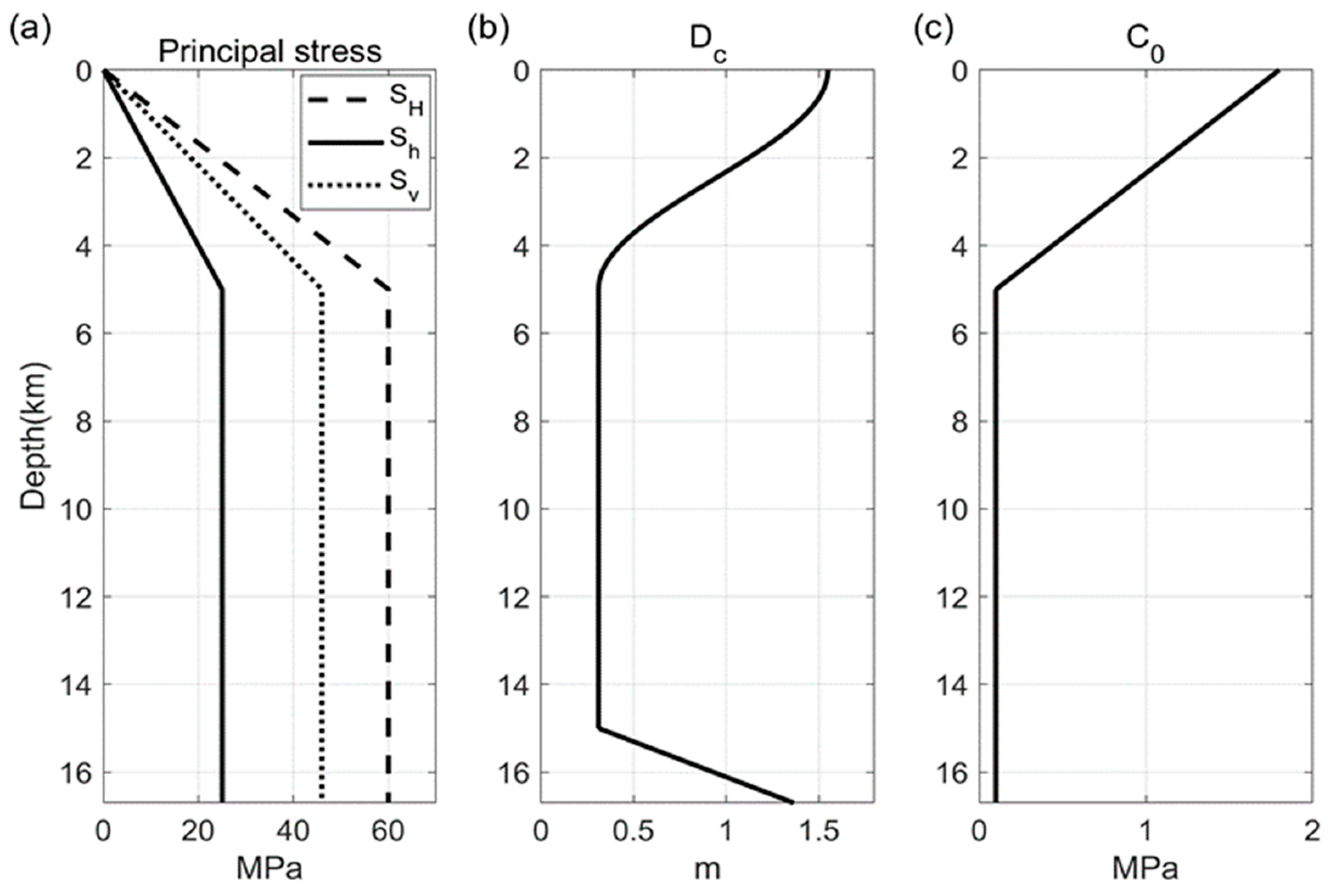
| Critical slip-weakening distance, (m) | 0.31 |
| Frictional cohesion, (MPa) | 0.10 |
| Element size, DH (m) | 50 |
| Nucleation patch radius, r (km) | 2.0 |
| Time step, DT (s) | 0.0027 |
| Maximum horizontal stress, SH (MPa) | 60.0 |
| Minimum horizontal stress, Sh (MPa) | 25.0 |
| Vertical stress, Sv (MPa) | 46.0 |
| SH Azimuth | N12°E |
Disclaimer/Publisher’s Note: The statements, opinions and data contained in all publications are solely those of the individual author(s) and contributor(s) and not of MDPI and/or the editor(s). MDPI and/or the editor(s) disclaim responsibility for any injury to people or property resulting from any ideas, methods, instructions or products referred to in the content. |
© 2025 by the authors. Licensee MDPI, Basel, Switzerland. This article is an open access article distributed under the terms and conditions of the Creative Commons Attribution (CC BY) license (https://creativecommons.org/licenses/by/4.0/).
Share and Cite
He, Z.; Zhang, Y.; Wang, W.; Wang, Z.; Sunilkumar, T.C.; Zhang, Z. Revisiting the 2020 Mw 6.8 Elaziğ, Türkiye Earthquake with Physics-Based 3D Numerical Simulations Constrained by Geodetic and Seismic Observations. Remote Sens. 2025, 17, 720. https://doi.org/10.3390/rs17040720
He Z, Zhang Y, Wang W, Wang Z, Sunilkumar TC, Zhang Z. Revisiting the 2020 Mw 6.8 Elaziğ, Türkiye Earthquake with Physics-Based 3D Numerical Simulations Constrained by Geodetic and Seismic Observations. Remote Sensing. 2025; 17(4):720. https://doi.org/10.3390/rs17040720
Chicago/Turabian StyleHe, Zhongqiu, Yuchen Zhang, Wenqiang Wang, Zijia Wang, T. C. Sunilkumar, and Zhenguo Zhang. 2025. "Revisiting the 2020 Mw 6.8 Elaziğ, Türkiye Earthquake with Physics-Based 3D Numerical Simulations Constrained by Geodetic and Seismic Observations" Remote Sensing 17, no. 4: 720. https://doi.org/10.3390/rs17040720
APA StyleHe, Z., Zhang, Y., Wang, W., Wang, Z., Sunilkumar, T. C., & Zhang, Z. (2025). Revisiting the 2020 Mw 6.8 Elaziğ, Türkiye Earthquake with Physics-Based 3D Numerical Simulations Constrained by Geodetic and Seismic Observations. Remote Sensing, 17(4), 720. https://doi.org/10.3390/rs17040720