Estimation of Aboveground Biomass of Chinese Milk Vetch Based on UAV Multi-Source Map Fusion

Abstract

Chinese milk vetch (CMV), as a typical green manure in southern China, plays an important role in improving soil quality and partially substituting nitrogen chemical fertilizers for rice production. Accurately estimating the aboveground biomass (AGB) of CMV is crucial for quantifying the biological nitrogen fixation amount (BNFA) and assessing its viability as a nitrogen fertilizer alternative. However, the traditional estimation methods have low efficiency in field-scale evaluations. Recently, unmanned aerial vehicle (UAV) remote sensing technology has been widely adopted for AGB estimation. This study utilized UAV-based multispectral and RGB imagery to extract spectral (Sp), textural (Tex), and structural features (Str), comparing various feature combinations in AGB estimation for CMV. The results indicated that the fusion of spectral, textural, and structural features indicated optimal estimation performance across all feature combinations, resulting in R² values of 0.89 and 0.83 for model cross-validation and spatial transferability validation, respectively. The inclusion of textural and spectral features notably improved AGB estimation, indicated an increase of 0.15 and 0.14 in R² values for model cross-validation and spatial transferability validation, respectively, compared with relying on spectral features only. Estimation based exclusively on structural features resulted in R² values of 0.65 and 0.52 for model cross-validation and spatial transferability validation, respectively. The present study establishes a rapid and extensive approach to evaluate the BNFA of CMV at the full blooming stage utilizing the optimal AGB estimation model, which will provide an effective calculation method for chemical fertilizer reduction.

1. Introduction

The yearly seasonal fallow area encompasses 24.9 million hectares, which constitutes 25% of arable land in China [1]. Planting green manure crops on fallow areas significantly contributes to expanding fertilizer sources and enhancing soil nitrogen and organic matter levels. Chinese milk vetch (CMV, Astragalus sinicus L.) indicates robust winter growth capabilities, enriched with nitrogen, phosphorus, potassium, and trace elements. Prevalent in the Yangtze River basin, CMV is strategically cultivated in fallow fields after rice harvest. Subsequently, at the full blooming stage, CMV is incorporated into the soil to increase soil organic matter and thus substitute a portion of nitrogen chemical fertilizers. Previous research indicated that the CMV’s biological nitrogen fixation approximately contributes to 78% of the overall nitrogen accumulation, supplying 41–146 kg/ha of nitrogen for subsequent crops [2]. Consequently, CMV has the potential to substitute 20–40% of nitrogen fertilizers after incorporation [3]. The utilization of this natural nitrogen fertilizer substitute has triggered substantial studies on estimating the biological nitrogen fixation amount (BNFA) of CMV [4,5,6]. The nitrogen fixation capacity of CMV correlates with aboveground biomass (AGB), nitrogen content, and biological nitrogen fixation rate, with AGB emerging as the primary influencing factor. Therefore, accurately estimating the AGB of CMV becomes pivotal in evaluating its impact of CMV on soil fertility and optimizing nitrogen fertilizer application in rice fields.

Traditional approaches for estimating AGB and related physiological and biochemical parameters, such as field surveys and vegetation growth models, encounter notable limitations. Field surveys are time-consuming and susceptible to investigator bias. Additionally, the application of vegetation growth models requires many parameters and heavily depends on extensive field survey data for calibration. For example, the APSIM (Agricultural Production Systems Simulator) model requires detailed calibration of parameters related to photosynthetic and respiration rates, which are specific to plant species and environmental conditions [7,8]. These parameters need to be measured under controlled conditions, often requiring complex experimental setups [7,8,9,10]. Furthermore, there is currently no comprehensive explanation of the mechanisms by which extreme atmospheric conditions impact agricultural production, leading to lower accuracy in crop simulation under extreme agricultural climates [11,12]. Therefore, crop growth models need to be improved by incorporating appropriate empirical models tailored to different crops.

Fortunately, the recent emergence of unmanned aerial vehicle (UAV) remote sensing technology offers a promising alternative to traditional AGB estimation methods. UAV remote sensing has several advantages, including high-speed data acquisition, objectivity, quantifiability, and non-destructiveness [13,14,15]. This technological innovation has proven its efficiency and accuracy in estimating vegetation AGB and other physiological and biochemical indicators [14,16,17,18]. However, the application of UAVs also faces challenges, such as regulatory issues related to airspace restrictions and flight permissions, which can complicate deployment in certain regions. Additionally, battery capacity, though less of a concern, can limit flight duration and the area that can be covered in a single survey. Despite these challenges, solutions are emerging—regulatory frameworks are gradually evolving to accommodate UAV usage, and advancements in battery technology and energy-efficient systems are likely to extend flight times, making these limitations manageable rather than insurmountable [19,20].

A prevalent approach for estimating vegetation parameters through UAV remote sensing capitalizes on the interaction between vegetation and solar radiation. By establishing correlations between reflectance and physiological and biochemical indices, such as AGB, the estimation of these indices becomes attainable [10,13,15,17,21]. To improve accuracy and mitigate interference from non-vegetated features, researchers have introduced various vegetation indices, such as the normalized difference vegetation index (NDVI), normalized green–red difference index (NGRDI), modified chlorophyll absorption ratio index (MCARI), and simple ratio index (SR) [18,22,23,24,25]. This method, based on optical remote sensing, offers the advantages of requiring minimal parameters and featuring straightforward and accurate mathematical expressions [26,27]. However, in open field scenarios, optical remote sensing methods encounter challenges arising from various factors, including soil background, variations in vegetation structure during different growth periods, and sowing densities. These factors may result in saturation issues in optical measurements [28,29].

Being a creeping crop, the high-density sowing of CMV fosters intense competition among individual plants, resulting in alterations in plant morphology. These changes can influence canopy spectral information, internal plant structure, and the composition of AGB, leading to substantial variations. Given these considerations, it is necessary to develop a reliable remote sensing estimation method for the AGB of CMV, crucial for accurately capturing the spatial distribution and structural composition of CMV plants in open fields.

In recent years, the fusion of diverse modeling features has emerged as a pivotal strategy to improve AGB estimation. For example, textural features extracted from UAV imagery can autonomously capture spatial information in the images, regardless of color tones. Key texture features, such as variance, homogeneity, and contrast, are commonly used in this context. Variance reflects the image’s contrast level by measuring the intensity variation across neighboring pixels, homogeneity captures the uniformity of pixel intensities within the image, and contrast quantifies the difference in intensity between adjacent pixels. These texture features, when integrated into models, enhance the ability to discern vegetation characteristics and improve AGB estimation accuracy. This capability assists in discerning variations in the spatial distribution of vegetation, vegetation types, and densities [30,31], thereby improving the precision of AGB estimation [32,33,34]. Furthermore, UAVs equipped with light detection and ranging (LiDAR) technology can reconstruct 3D point cloud information of vegetation [14,35,36]. Structural features, such as vegetation plant height, canopy diameter, and canopy cover, derived from this 3D point cloud, facilitate efficient AGB estimation [37]. Despite its potential, the application of this method in precision agriculture management still encounters challenges related to technology costs. Nevertheless, advancements in the structure from motion (SFM) algorithm for motion recovery now enable the reconstruction of vegetation 3D point cloud information using low-cost, high-resolution RGB images [38]. This development allows for a cost-effective AGB estimation [39,40,41]. Moreover, the fusion of structural and spectral features has progressively proven to be an effective approach for enhancing the accuracy of vegetation AGB estimation [42,43]. Additionally, the comprehensive fusion of spectral, structural, and image textural features captures the spatial distribution and growth status of vegetation, contributing to further improvements in AGB estimation performance [16,44].

Previous studies underscore the effectiveness of UAV multi-source map fusion technology in improving AGB estimation through the resolution of optical measurement saturation challenges. However, no investigations have applied this technique to CMV. A comprehensive examination is imperative to assess the applicability and spatial transferability of this optimization methodology in the AGB estimation of CMV, given its prostrate growth and high-density sowing. Hence, this study aims to (1) quantitatively evaluate the impact of UAV-based spectral, textural, and structural features on the AGB of CMV modeling and (2) ascertain the efficacy of various feature combinations in mitigating optical remote sensing saturation during modeling. Through the construction of an optimized AGB estimation model, this study contributes to the large-scale rapid estimation of BNFA, thus optimizing the fertilizer application practice in the CMV-rice rotation system.

2. Materials and Methods

2.1. Study Area

The study area was in Taihu Farm, Jingzhou City, Hubei Province, China (30°21′N, 112°02′E), with an average annual temperature of 16.3 °C and an annual rainfall of 1200 mm (Figure 1). The study area implemented a CMV-rice rotation system, where rice was cultivated as a single-season crop and CMV was grown during the winter fallow period. The CMV variety was Yijiang (Wuhu Qing Yijiang Seed Industry Co., Ltd., Wuhu, China), and the seeds were sown uniformly at a rate of 30 kg/ha. No chemical fertilizers or irrigation were applied during the CMV growth period.

This study was conducted in two specified regions identified as Field East and Field West, both located at Taihu Farm. The fields share similar conditions in terms of sunlight, air temperature, irrigation, and soil characteristics. Each study field was subdivided into 96 plots, measuring 32 m² (4 m × 8 m) for Field East and 20 m² (4 m × 5 m) for Field West, respectively, with 30 cm wide ridges separating the plots. The field trial was set up in 2015 to evaluate the effect of CMV incorporation on soil fertility and rice growth. The primary objective of the current investigation was to develop a model for estimating the AGB of CMV using remote sensing technology. Consequently, data acquisition exclusively focused on plots with CMV cultivation. Specifically, 75 plots from Field East were selected for constructing the AGB estimation model of CMV and conducting cross-validation, while 48 plots from Field West were chosen for the spatial transferability validation.

2.2. Overall Workflow

The workflow comprises five key components: image preprocessing, feature extraction, feature selection, feature combination, model construction, and spatial transferability validation (Figure 2).

2.3. Ground Data Acquisition and Processing

(1)

Ground-based measurement of CMV plant height

Ground truth plant height data were measured on 13 April 2021, during the full blooming stage of CMV. Initially, a sample plot with dimensions of 30 cm × 30 cm was randomly chosen from each plot, and the precise count of CMV plants within it was documented. Following this, ten representative plants were selected from the plot, and the height of fully extended plants was gauged using a telescopic ruler. The average of these measurements was regarded as the plant height value (in centimeters) for the respective plot.

(2)

Ground-based measurement of the AGB of CMV

Ground data measurement ensued after acquiring actual plant height measurements on the same day. All CMV plants were exclusively harvested within each plot, and the fresh weight meticulously recorded to determine the AGB of CMV in kg/m² for the respective plot.

(3)

Ground-based measurement of CMV moisture content and nitrogen content

For each plot, approximately 500 g of harvested CMV samples were taken and subjected to fresh weight measurement. Subsequently, the samples were dried in an oven (initially at 105 °C for the first 30 min) until a constant weight was achieved at 70 °C. The measured dry weight facilitated the calculation of moisture content (%) for the CMV. Following this, the plant samples were ground and digested with H₂SO₄-H₂O₂. The nitrogen content (%) was then measured using the Kjeldahl method. The data on moisture and nitrogen contents were utilized for the estimation of BNFA (kg/ha).

2.4. UAV Image Data Acquisition and Processing

To ensure consistency between UAV remote sensing data and ground-based data, RGB and multispectral images were acquired using DJI Mavic 2 Pro and P4 multispectral quadcopter UAVs between 11:00 and 13:00 on the day of ground data acquisition.

The Mavic 2 Pro, designed for commercial applications, is a lightweight drone equipped with an advanced omnidirectional vision system, infrared sensors, and a high-precision anti-shake gimbal. It features a 20-megapixel CMOS sensor, a 24 mm focal length lens, and an 85° angle of view for high-resolution RGB image capture. Similarly, the P4 multispectral, tailored for multispectral imaging, shares key features with the Mavic 2 Pro. It incorporates a multi-directional vision system, an infrared sensor system, and a high-precision anti-shake gimbal with a built-in real-time kinematic (RTK) system. Equipped with six CMOS image sensors, the P4 multispectral captures images in five wavelength bands: blue (450 ± 16 nm), green (560 ± 16 nm), red (650 ± 16 nm), red edge (730 ± 16 nm), and near-infrared (840 ± 16 nm). Each monochrome sensor features 2.12 million pixels, a lens focal length of 40 mm, and a viewing angle of 62.7°.

All aerial missions occurred under optimal weather conditions, including clear skies, minimal wind, at an altitude of 20 m, and a speed of 2 m/s. Images were acquired at regular 2 s intervals. The flight grid was a single grid, and both the forward and side overlaps were set to 80%, ensuring adequate coverage between images and improving the accuracy of image stitching. Flight paths covered the entire study area, and radiometric calibration panels were strategically placed within the flight coverage. For radiometric calibration, the empirical linearization radiometric calibration (ELRC) method [45] (Farrand et al., 1994) was applied to ensure accuracy and consistency of radiometric values acquired by the multispectral sensors during flights. Additionally, ten ground control points (GCPs) were positioned within each study field for precise georeferencing. Horizontal measurements of the GCPs’ geographic coordinates were conducted using a GNSS device based on RTK technology, providing precise locations for geometric correction of images. Moreover, RGB images of the study area were acquired during the bare ground period between 11:00 and 13:00 on 18 September 2020. These images were utilized for generating a digital elevation model (DEM) representing the bare ground period after rice harvest and before CMV sowing.

2.4.1. Image Mosaic and Radiometric Calibration

In this study, the UAV multispectral and RGB images from the two study fields were mosaiced using Agisoft Metashape 1.8.0 software. Subsequently, radiometric calibration was performed on the multispectral images using the ELRC method.

$$\begin{array}{c}{R}_i={DN}_i+{Gain}_i+{Offset}_i\left(\mathrm{i}=\mathrm{1,2}\dots 5\right)\end{array}$$

(1)

$$\left(\begin{array}{c}0.10\\ 0.30\\ 0.60\end{array}\right)=\left(\begin{array}{c}{\displaystyle \genfrac{}{}{0pt}{}{{DN}_{0.10}}{{DN}_{0.30}}}\\ {DN}_{0.60}\end{array}\right)\times {Gain}_i\times {Offset}_i$$

(2)

Note: R_i and DN_i represent the surface reflectance and gray value of a specific pixel in the i-th band. The gain and offset values for the i-th band are constants derived from experimental measurements, considering the reflectance characteristics of diverse radiometric calibration targets.

2.4.2. Removal of Soil Background

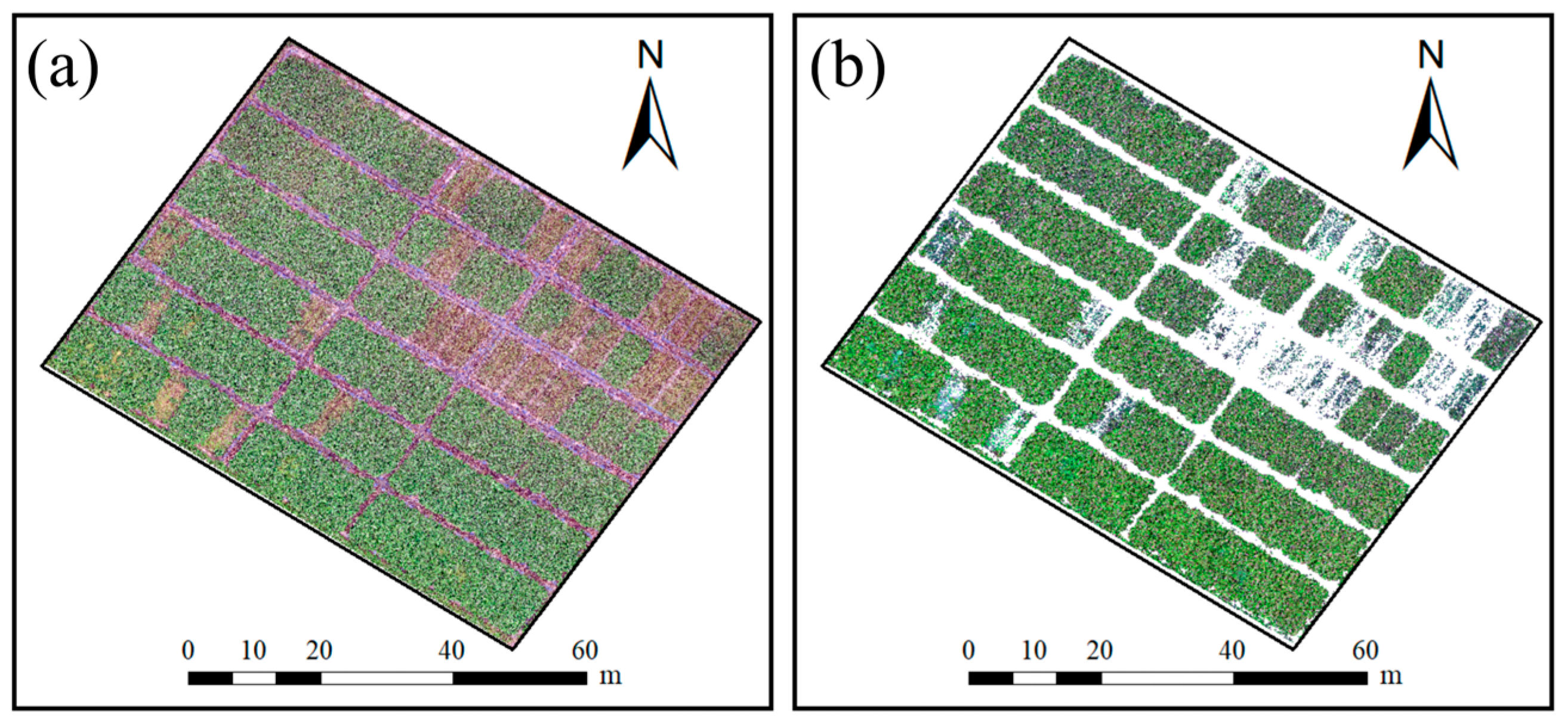
In the quantitative assessment of vegetation physiological and biochemical indices, non-vegetative elements, such as soil may distort radiometric data of vegetation targets, lowering accuracy in information extraction. To mitigate this, removing soil background from remote sensing images is crucial before extracting vegetation-related data. ArcGIS 10.8 and ENVI 5.3 were used in this study for soil background removal from radiometrically calibrated multispectral and RGB images. Figure 3 shows multispectral images before and after soil removal (similarly for RGB images). A soil background mask was constructed through supervised classification using an SVM classifier, with visual interpretation markers established simultaneously. Ten thousand random sample points for soil and vegetation were selected to evaluate the SVM classifier’s performance. Classification results indicated overall accuracies of 95.43% for soil and 93.36% for vegetation in both multispectral and RGB images (Figure 4). The validated soil background mask was then exported as a vector file, facilitating soil background removal from the images.

2.4.3. Extraction of Spectral, Textural, and Structural Features

In the study area, a rectangular region of interest (ROI) was defined for multispectral and RGB images based on plot areas to extract spectral, structural, and textural features. To mitigate edge effects, ROI dimensions were set 0.2 m smaller than the original plots. Spectral, structural, and textural features were extracted using the “zonal statistics as table” function from the ArcPy library. Twelve vegetation indices, widely recognized for AGB estimation, were selected as spectral features. Corresponding spectral feature images were systematically computed using the geospatial data abstraction library (GDAL) in Python (version 3.10). The calculation formulas are presented in

Table 1. Spectral features of the present study.

Spectral	Formula	Reference
NDVI (Normalized Difference Vegetation Index)	${\displaystyle \frac{NIR-R}{NIR+R}}$	[46]
SR (Simple Ratio Index)	${\displaystyle \frac{NIR}{R}}$	[47]
GRDVI (Green Re-normalized Different Vegetation Index)	${\displaystyle \frac{NIR-G}{\sqrt{NIR+G}}}$	[48]
NDRE (Normalized Difference RedEdge Index)	${\displaystyle \frac{NIR-RE}{NIR+RE}}$	[49]
CIgreen (Green Chlorophyll Index)	${\displaystyle \frac{NIR}{G}}-1$	[50]
CIRE (ChlorophyII Index-RedEdge)	${\displaystyle \frac{NIR}{RE}}-1$	[50]
CLI (Green Leaf Index)	${\displaystyle \frac{2\times G-R-B}{2\times G+R+B}}$	[51]
GNDVI (Green Normalized Difference Vegetation Index)	${\displaystyle \frac{NIR-G}{NIR+G}}$	[52]
NGRDI (Normalized Green–Red Difference Index)	${\displaystyle \frac{G-R}{G+R}}$	[53]
NPCI (Normalized Pigment Chlorophyll Ratio Index)	${\displaystyle \frac{R-B}{R+B}}$	[54]
VARIRE (Visible Atmospherically Re-sistant Index-RedEdge)	${\displaystyle \frac{RE-1.7\times R+0.7\times B}{RE+2.3\times R-1.3\times B}}$	[55]
LCI (Leaf Chlorophyll Index)	${\displaystyle \frac{NIR-RE}{NIR+RE}}$	[56]

.

Textural features based on the gray level co-occurrence matrix (GLCM) using ENVI 5.3 included eight metrics: mean (Mean), variance (Var), homogeneity (Hom), contrast (Con), dissimilarity (Dis), entropy (En), second moment (Sm), and correlation (Cor). For multispectral images, forty textural features were calculated across five bands. The second-order probabilistic statistical filter used default settings with a 3 × 3 window size and a diagonal direction of [1, 1]. Calculation formulas are presented in

Table 2. Textural features of the present study.

Textural	Formula	Description
Mean	${\displaystyle \sum _i}{\displaystyle \sum _j}x(i,j)p(i,j)$	Average situation of gray value
Variance	${\displaystyle \sum _i}{\displaystyle \sum _j}{(i-u)}^{2}p(i,j)$	Degree of change of gray value
Homogeneity	${\displaystyle \sum _i}{\displaystyle \sum _j}{\displaystyle \frac{1}{1+{(i-j)}^2}}p(i,j)$	Local texture homogeneity
Contrast	${\displaystyle \sum _{n=0}^{N_g-1}}{n}^2{\left\{{\displaystyle \sum _{i=1}^{N_g}}{\displaystyle \sum _{j=1}^{N_g}}p(i,j)\right\}}_{\left|i-j\right|=n}$	Texture clarity
Dissimilarity	${\displaystyle \sum _{n=1}^{N_g-1}}n{\left\{{\displaystyle \sum _{i=1}^{N_g}}{\displaystyle \sum _{j=1}^{N_g}}{p(i,j)}^2\right\}}_{\left|i-j\right|=n}$	Texture information similarity
Entropy	$-{\displaystyle \sum _i}{\displaystyle \sum _j}p(i,j)\mathit{log}\left(p\right(i,j\left)\right)$	Texture complexity and non-uniformity
Second moment	$-{\displaystyle \sum _i}{\displaystyle \sum _j}{p(i,j)}^2$	Roughness of texture and uniformity of image gray distribution
Correlation	${\displaystyle \frac{{\sum }_i{\sum }_j\left(ij\right)p\left(i,j\right)-{\mu }_x{\mu }_y}{{\sigma }_x{\sigma }_y}}$	Texture consistency
Mean	${\displaystyle \sum _i}{\displaystyle \sum _j}x(i,j)p(i,j)$	Average situation of gray value
Variance	${\displaystyle \sum _i}{\displaystyle \sum _j}{(i-u)}^{2}p(i,j)$	Degree of change of gray value

Note: In the equation, N_g represents the gray level, i represents the grayscale value at point (x, y), and j represents the grayscale value at another point located at a distance d from the point (x, y). p (i, j) represents the frequency of occurrence of pixels with grayscale value j at a distance d from the point (x, y); u represents the average of all gray values in the image area. μ_x and μ_y represent the mean texture values in the x and y directions, respectively, while μ_x and μ_y represent the standard deviations in the x and y directions.

.

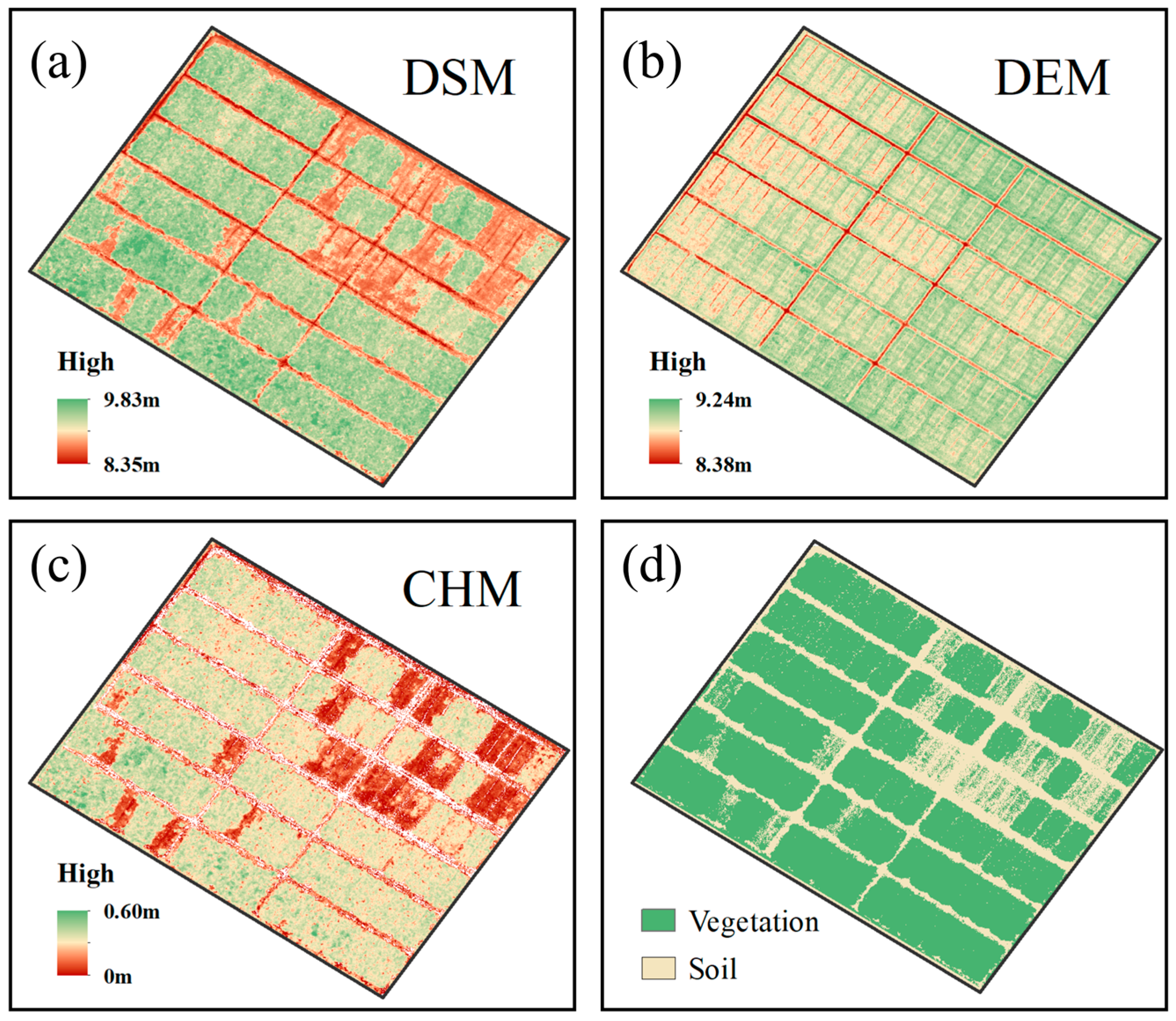
Utilizing the SFM algorithm to reconstruct 3D point cloud information from RGB images provides elevation details for the study area. However, its accuracy is limited, offering only vegetation canopy elevation information rather than precise plant height. To overcome this limitation, the study aims to determine the bare ground height of the study field, crucial for accurate plant height information. After the rice harvest on 18 September 2020, RGB images were acquired to generate the DEM of the study area (Figure 5b). Subsequently, the DSM (Figure 5a), derived from RGB images during the CMV full blooming stage, underwent raster subtraction with the DEM, resulting in the specific CMV canopy height model (CHM) (Figure 5c). Finally, the soil background mask from Section 2.4.2 was applied to eliminate soil pixels from the CHM, ensuring more accurate plant height information and laying the foundation for subsequent feature extraction.

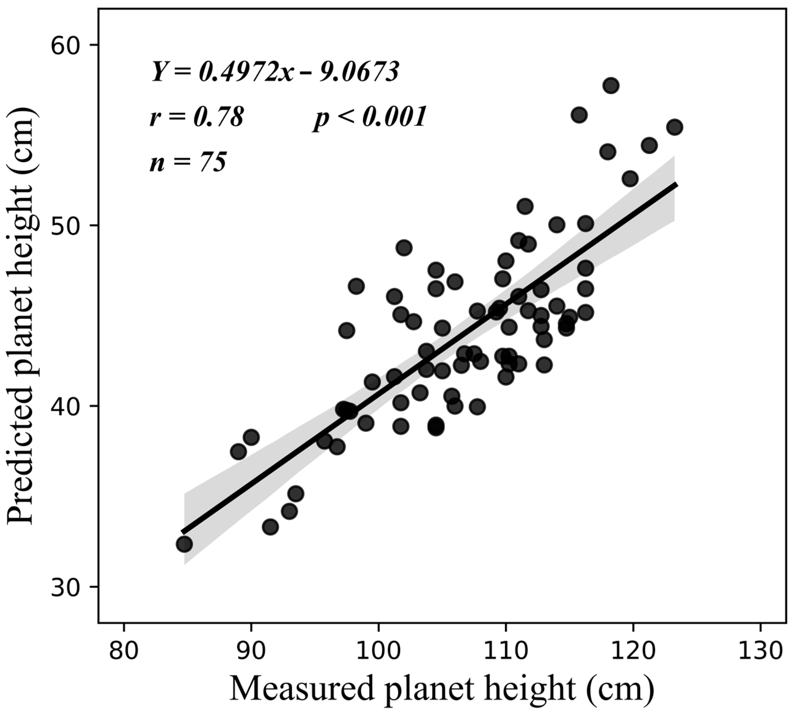
Validating the extracted plant height from the CHM is crucial for ensuring accuracy and reliability in practical applications. In this study, linear regression analysis was utilized to examine the correlation between the estimated plant height from CHM and the measured ground plant height. Figure 6 indicates a robust correlation (r = 0.78, p < 0.001), confirming the reliability of the CHM-extracted plant height for subsequent extraction of vegetation structure features.

Methods using volumetric pixels and cylindrical surface fitting models 3D vegetation canopy structures with optimal cylindrical shapes derived from LiDAR or photogrammetric point clouds to extract vegetation volume in diverse environments, such as forests and shrubs [57,58]. However, the 3D point cloud generated from RGB images and SFM algorithms has limitations, capturing only outer canopy volume (CV) and lacking information about the internal structure of complex vegetation growth [59]. To overcome this, our study employed the surface difference method to calculate canopy volume. This method involves determining the volume between the highest and lowest points of the canopy based on the CHM. The CV for each plot was computed as the product of the extracted plant height and the number of vegetation pixels within the plot [60,61].

Ultimately, four structural features were extracted using the CHM: mean plant height (PH_mean), standard deviation of plant height (PH_std), coefficient of variation of plant height (PH_cv), CV, and plot-scale canopy cover (CC) derived through vegetation and soil classification masks [17]. PH_std and PH_cv are employed to characterize the vertical structure complexity of vegetation [62]. These structural features offer a quantitative depiction of the vertical vegetation structure. The calculation formulas are presented in

Table 3. Structural features of the present study.

Structural	Formula
Mean plant height (PHmean) (cm)	${\displaystyle \frac{1}{n}}\times {\sum }_{i=1}^n{H}_i$
Standard deviation of plant height (PHstd) (cm)	$\sqrt{{\displaystyle \frac{1}{n-1}}\times {\sum }_{i=1}^n{H}_i-{PH}_{mean}}$
Coefficient of variation of plant height (PHcv) (%)	${PH}_{std}/{PH}_{mean}$
Canopy Volume (CV) (m3/pixel3)	${\sum }_{i=1}^n{A}_i\times H_i$
Canopy cover (CC) (%)	${Canopy}_{pixels}/{ROI}_{pixels}$

Note: i represents the i-th pixel in the CHM, n represents the number of vegetation pixels within the plot, A_i represents the area of the i-th pixel, H_i represents the height of the i-th pixel, and ROI_pixels represents the total number of pixels within the ROI.

.

2.5. Selection and Fusion of Features

Pearson correlation analysis quantifies the linear correlation strength between two variables, commonly applied in exploratory data analysis. It calculates the correlation coefficient (“r”) as the ratio of the product of variable covariance to their standard deviation. The coefficient (“r”) ranges from −1 to 1, with a larger absolute value indicating a stronger correlation. Variable selection using random forests (VSURF) is a feature selection technique based on the random forests algorithm (RF) [63] (Genuer et al., 2010). 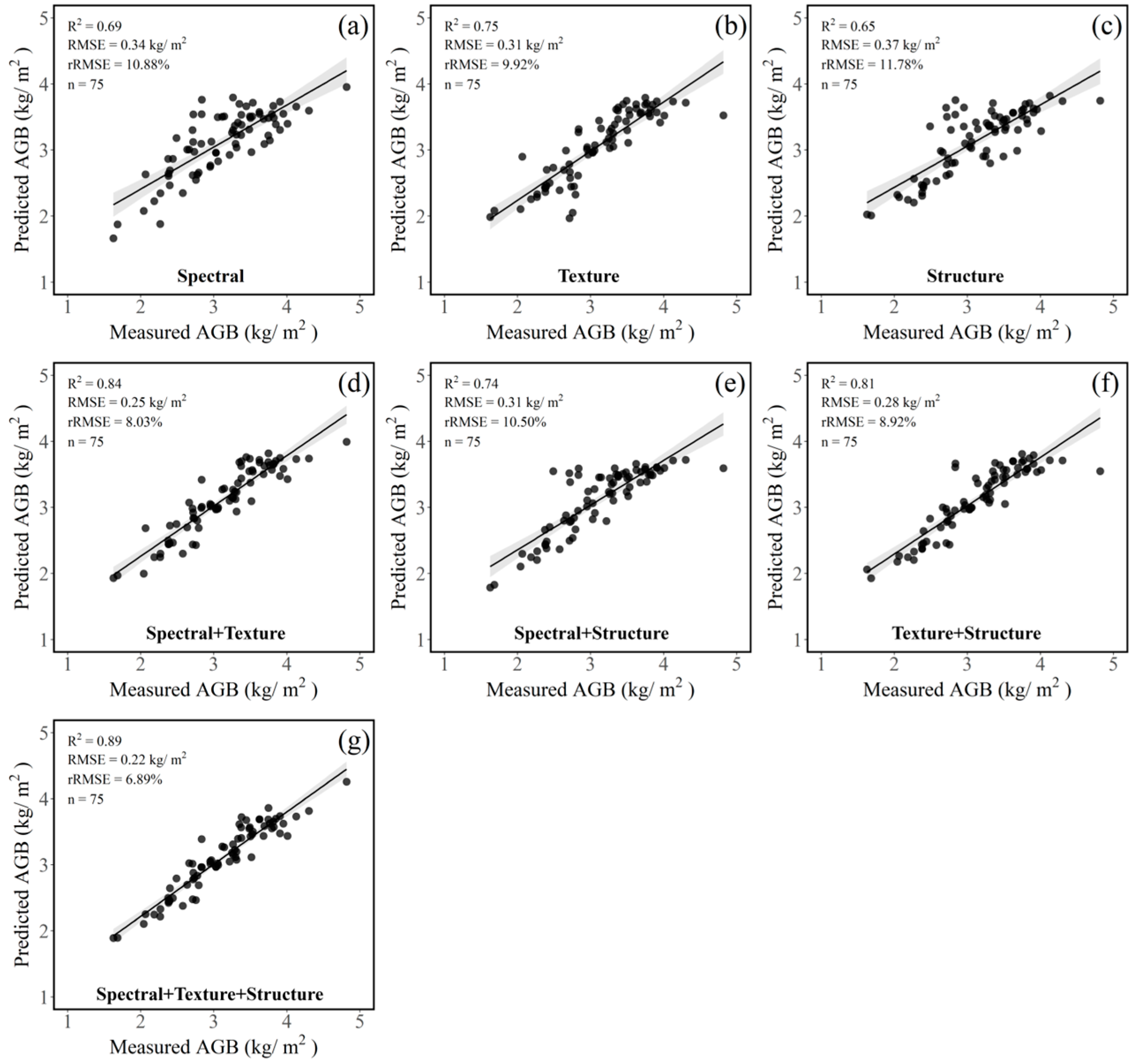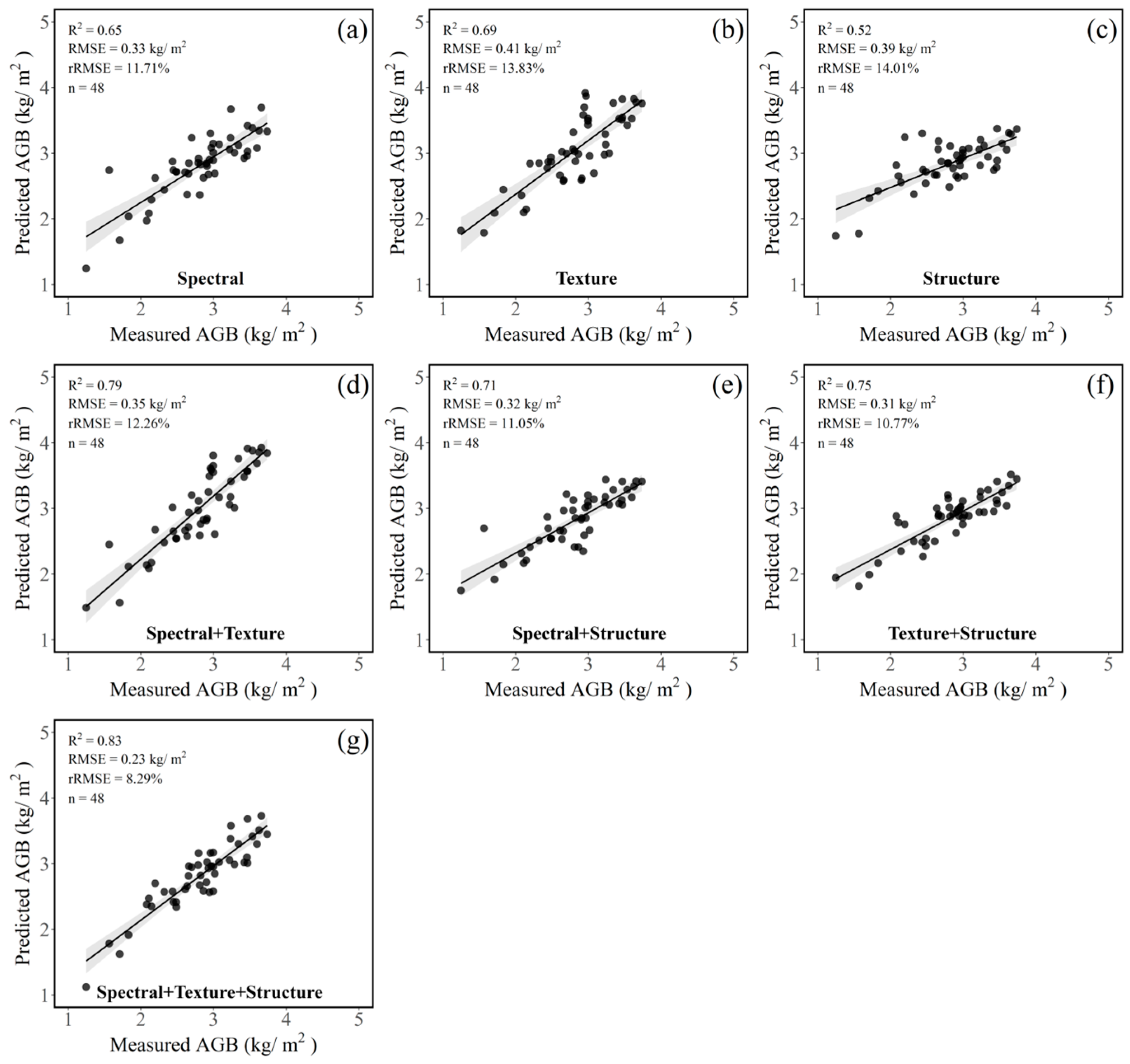It efficiently selects crucial features from a vast pool, addressing model uncertainty and multiple covariance issues [64,65]. In this study, RStudio 1.4 (R 4.2.0) and the R language library VSURF were employed for feature selection. The feature selection process occurred sequentially in this study using Pearson and VSURF for all feature types. Seven feature combinations were established for the retained features: Sp, Tex, Str, Sp + Tex, Sp + Str, Tex + Str, and Sp + Tex + Str.

2.6. Model Evaluation and AGB, BNFA Mapping

In this study, the Python Scikit-learn library was employed to construct an AGB estimation model for CMV using the RF algorithm. Grid search optimization focused on key hyperparameters, such as the number of decision trees (n_estimators), maximum tree depth (max_depth), maximum features at each split (max_features), minimum samples required for leaf nodes (min_samples_leaf), and internal nodes of a tree (min_samples_split). The process involved defining a hyperparameter space, systematically adjusting parameters, and determining the set that maximized accuracy on the model validation set. Model performance was assessed through repeated k-fold cross-validation and spatial transferability validation, using evaluation metrics, including the coefficient of determination (R²), root mean square error (RMSE), and relative root mean square error (rRMSE). A more robust model is indicated by higher R² and lower RMSE and rRMSE values (Equations (3)–(5)).

$$\begin{array}{c}\begin{array}{c}{R}^2=1-{\displaystyle \frac{{\sum }_{i=1}^n{\left(y_i-{\widehat{y}}_i\right)}^2}{{\sum }_{i=1}^n{\left(y_i-\overline{y}\right)}^2}}\end{array}\end{array}$$

(3)

$$\begin{array}{c}RMSE=\sqrt{{\displaystyle \frac{1}{n}}{\sum }_{i=1}^n{\left(y_i-{\widehat{y}}_i\right)}^2}\end{array}$$

(4)

$$\begin{array}{c}rRMSE=\left({\displaystyle \frac{\sqrt{\frac{1}{n}{\sum }_{i=1}^n{\left(y_i-{\widehat{y}}_i\right)}^2}}{\frac{1}{n}{\sum }_{i=1}^n{y}_i}}\right)\times 100\%\end{array}$$

(5)

Note: n represents the number of samples, y_i represents the measured AGB value of the i-th sample, ŷ_i represents the predicted AGB value of the i-th sample, and ȳ represents the average measured AGB value.

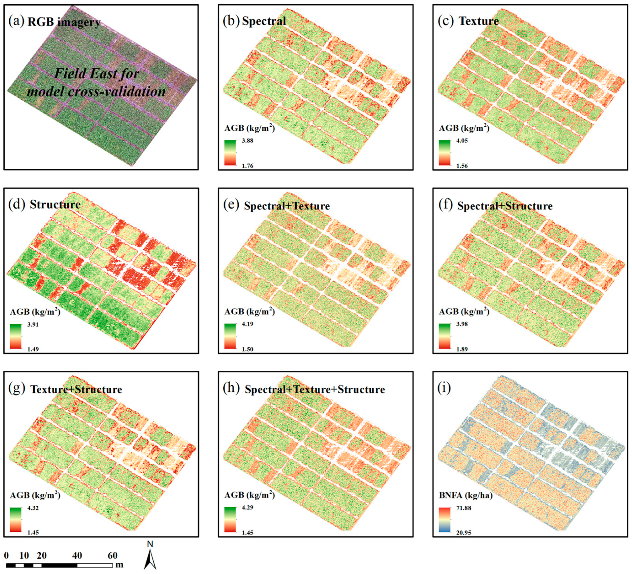
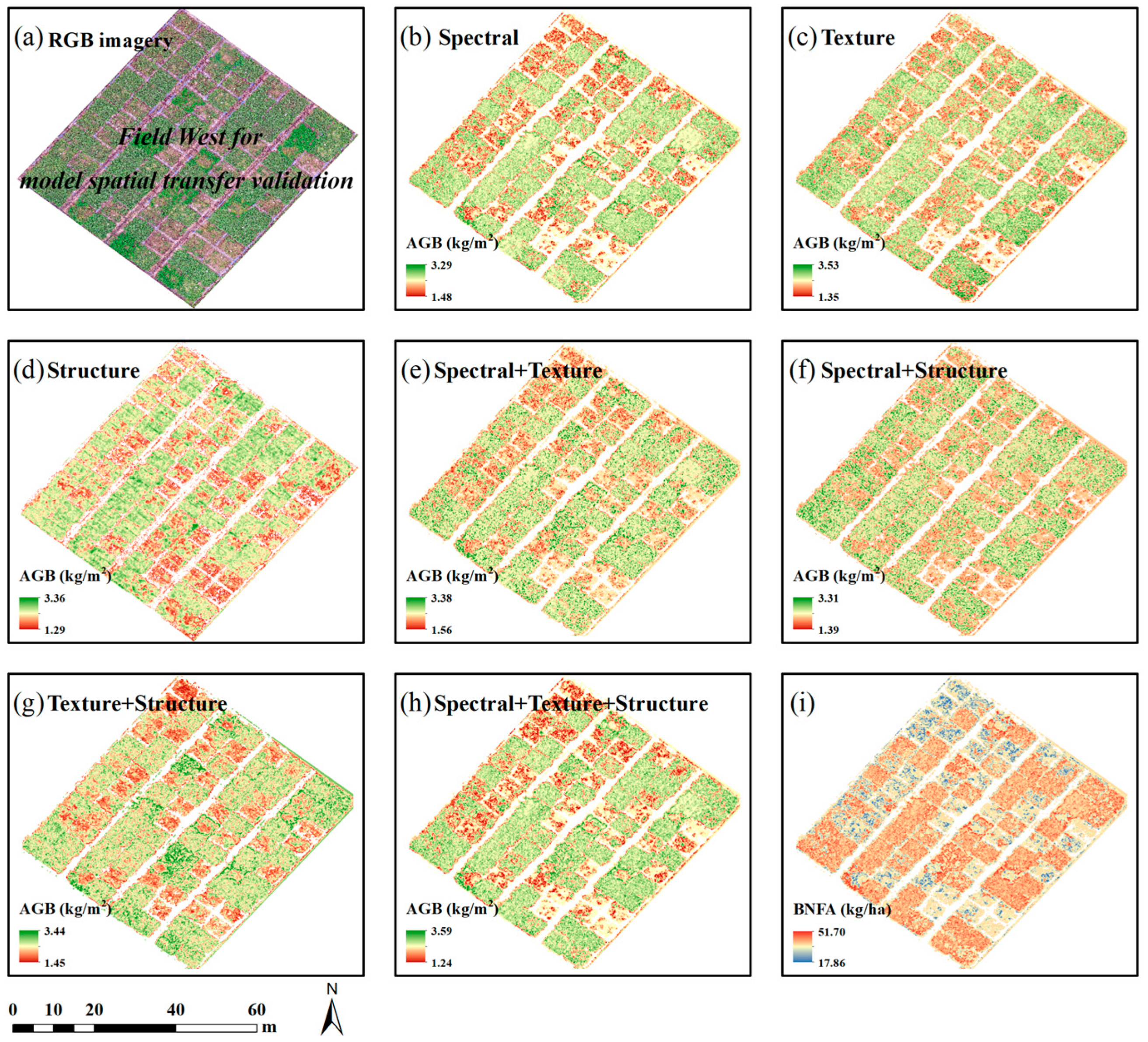
In this study, the AGB estimation model was constructed under various feature combination settings and employed to generate AGB estimation maps for CMV. Subsequently, the BNFA of CMV was calculated with the biological nitrogen fixation rate of 66% [66] (Bolger et al., 1995). The formula is presented below:

$$\begin{array}{c}\begin{array}{c}BNFA=AGB\times \left(1-MC\%\right)\times N\%\times BNF\%\times {10}^4\end{array}\end{array}$$

(6)

Note: BNFA represents the biological nitrogen fixation amount (kg/ha), AGB represents the aboveground fresh weight of CMV (kg/m²), MC% represents the moisture content (%), N% represents the nitrogen content (%), and BNF% represents the rate of biological nitrogen fixation (%). The average values for BNF%, MC%, and N% were measured from the field studies (i.e., 66%, 87.76%, and 2.03%), and 10⁴ represents the unit conversion.

3. Results

3.1. Selected Features for AGB Modeling

(1)

Spectral features

The Pearson coefficients, indicating the correlation between the AGB of CMV and the 12 spectral features derived from UAV multispectral images, are presented in

Table 4. Pearson’s correlation coefficient (r) for multispectral image spectral features and the AGB of CMV in Field East (n = 75).

Spectral	Correlation Coefficient (r)	Spectral	Correlation Coefficient (r)
NDVI	0.71 **	GLI	0.72 **
SR	0.70 **	GNDVI	0.74 **
GRDVI	0.75 **	NGRDI	0.62 **
NDRE	0.65 **	NPCI	−0.64 **
CIgreen	0.76 **	VARIRE	0.71 **
CIRE	0.63 **	LCI	0.67 **

Note: ** p < 0.01.

. The results indicate that the majority of spectral features exhibit a strong correlation with AGB (|r| > 0.7, p < 0.01), except for NDRE, CIRE, NGRDI, NPCI, and LCI. Particularly, CI_green shows the highest correlation with AGB (r = 0.76, p < 0.05), while NGRDI exhibits the lowest correlation (|r| = 0.62, p < 0.01). Subsequently, seven spectral features indicating high correlation with AGB (|r| > 0.7, p < 0.05) were selected for the second period of VSURF feature selection. After the initial Pearson-based selection, these features underwent further refinement using VSURF, resulting in the final selected features: CI_green, GNDVI, GRDVI, SR, and GLI.

(2)

Textural features

Table 5. Pearson’s correlation coefficient (r) for multispectral image textural features and the AGB of CMV in Field East (n = 75).

Textural	Correlation Coefficient (r)	Textural	Correlation Coefficient (r)
B-Mean	0.39 **	R-Dis	0.34 **
B-Var	0.34 **	R-En	0.21 NS
B-Hom	−0.33 **	R-Sm	−0.2 NS
B-Con	0.38 **	R-Cor	−0.29*
B-Dis	0.36 **	RE-Mean	0.59 **
B-En	0.30 **	RE-Var	−0.27 *
B-Sm	−0.31 *	RE-Hom	0.32 **
B-Cor	−0.52 **	RE-Con	−0.21 NS
G-Mean	0.54 **	RE-Dis	−0.26 *
G-Var	0.54 **	RE-En	−0.18 NS
G-Hom	−0.59 **	RE-Sm	0.17 NS
G-Con	0.56 **	RE-Cor	−0.80 **
G-Dis	0.57 **	NIR-Mean	0.61 **
G-En	0.61 **	NIR-Var	−0.64 **
G-Sm	−0.61 **	NIR-Hom	0.76 **
G-Cor	−0.41 **	NIR-Con	−0.62 **
R-Mean	−0.44 **	NIR-Dis	−0.68 **
R-Var	0.37 **	NIR-En	−0.77 **
R-Hom	−0.26 *	NIR-Sm	0.77 **
R-Con	0.38 **	NIR-Cor	−0.82 **
B-Mean	0.39 **	R-Dis	0.34 **
B-Var	0.34 **	R-En	0.21 NS
B-Hom	−0.33 **	R-Sm	−0.2 NS
B-Con	0.38 **	R-Cor	−0.29 *

Note: * p < 0.05, ** p < 0.01, and NS: represents not significant correlation with p-value < 0.05.

indicates that, among all textural features, except for five features (R-En, R-Sm, RE-Con, RE-En, RE-Sm) that exhibit no significant correlation with AGB. The remaining 35 features demonstrate a noteworthy correlation with AGB (p < 0.05). In this study, strong correlations with AGB (|r| > 0.6) were identified and retained from the aforementioned 35 features, resulting in a total of 11 textural features. Among these, NIR-Cor exhibits the highest correlation with AGB (r = −0.82, p < 0.05), and all eight textural features extracted based on the NIR band show strong correlations with AGB. Following the initial selection by Pearson, these 11 textural features underwent further refinement using VSURF, ultimately yielding the final modeling features: RE-Cor, NIR-Con, NIR-Sm, and NIR-En.

Table 6. Pearson’s correlation coefficient (r) for multispectral image structural features and the AGB of CMV in Field East (n = 75).

Structural	Correlation Coefficient (r)
PHmean	0.57 **
PHstd	−0.21 NS
PHcv	−0.60 **
CV	0.54 **
CC	0.66 **

Note:, ** p < 0.01, and NS: represents not significant correlation with p-value < 0.05.

indicates the results of the Pearson correlation analysis conducted on the five structural features extracted from RGB images and the AGB of CMV. Following the analysis, it was observed that the correlation between PH_std and AGB lacked significance, leading to its exclusion from the selected structural features. The remaining four structural features (PH_mean, PH_cv, CV, and CC) exhibited a correlation with AGB beyond the moderate level, prompting their retention as part of the Str feature combination. To maintain a balance among different feature types, the remaining four structural features did not undergo VSURF feature selection.

Table 7. Features selected through a two-step selection process.

Feature Type	Number of Input Features	Pearson Filters the Retained Features			VSURF Filters Retained Features
Spectral	12	NDVI	SR	GRDVI	SR	GRDVI
		CIgreen	GLI	GNDVI	CIgreen	GLI
		VARIRE			GNDVI
Textural	40	G-En	G-Sm	RE-Cor	RE-Cor	NIR-Con
		NIR-Mean	NIR-Var	NIR-Hom	NIR-Sm	NIR-En
		NIR-Con	NIR-Dis	NIR-Cor
		NIR-En	NIR-Sm
Structural	5	PHmean	PHcv	CV
		CC

presents the results of Pearson correlation analysis and VSURF selection, resulting in the selection of five spectral features and four textural features from the initial 12 spectral features and 40 textural features. These chosen features serve as inputs for training the RF model, along with the four structural features retained after the Pearson correlation analysis selection.

3.2. Evaluation of AGB Estimation Models Using Various Feature Combinations

Based on the results of feature selection in Section 3.1 and feature combination settings in Section 2.5, the AGB estimation model utilizing the RF algorithm is constructed. Figure 7 shows the cross-validation scatter plot, while Figure 8 displays the scatter plot for spatial transferability validation.

Figure 7 indicates the performance of various feature combinations in modeling the AGB of CMV. Among models constructed with a single type of features, the Tex-based model indicates the best performance (R² = 0.75, RMSE = 0.31 kg/m², rRMSE = 9.92%), followed by the Sp-based model (R² = 0.69, RMSE = 0.34 kg/m², rRMSE = 10.88%), while the Str-based model performs relatively poorly (R² = 0.65, RMSE = 0.37 kg/m², rRMSE = 11.78%). The Sp + Tex combination (Figure 7d) significantly improves model performance (R² = 0.84, RMSE = 0.25 kg/m², rRMSE = 8.11%). Additionally, the combination of three types of features (Sp + Tex + Str) results in a substantial improvement in model accuracy (R² = 0.89, RMSE = 0.22 kg/m², rRMSE = 6.89%).

In summary, a model constructed based on a single type of features, Sp or Tex, can achieve high estimation accuracy, while the Str-based model has lower accuracy. Combining two types of features improves accuracy to some extent, while combining all three features leads to a significant increase in model accuracy.

Figure 8 indicates the results of spatial transferability validation for the AGB estimation model with different feature combinations. Similarly, the model with a combination of three types of features (Sp + Tex + Str) performs the best (R² = 0.83, RMSE = 0.23 kg/m², rRMSE = 8.29%).

3.3. Mapping Results for AGB and BNFA

In this section, AGB maps for both Field East and Field West (Figure 9b–h and Figure 10b–h) were generated using AGB estimation models incorporating various feature combinations. Upon visual examination of the RGB orthophotographs (Figure 9a and Figure 10a) and the resulting AGB maps, a consistent spatial distribution pattern with CMV growth conditions and bare plot height was observed. Specifically, the AGB map generated from the optimal estimation model for Field East indicated a spatial trend with higher values in the south, lower in the north, higher in the west, and lower in the east. The AGB values ranged from 1.45 to 4.29 kg/m². Similarly, the AGB map based on the optimal estimation model for Field West indicated a spatial trend with higher values in the south, lower in the north, higher in the east, and lower in the west, with AGB values ranging from 1.24 to 3.59 kg/m².

Furthermore, employing the best estimation model in conjunction with ground-based data (including plot-specific moisture content, nitrogen content, and a 66% biological nitrogen fixation rate measured from previous studies in the same study field), BNFA mapping for CMV in the study field was accomplished (Figure 9i and Figure 10i). The BNFA distributions for Field East and Field West aligned with the spatial patterns of AGB on their respective AGB maps generated from the best estimation model, ranging from 20.95 to 71.88 kg/ha and 17.86 to 51.70 kg/ha, respectively.

4. Discussion

4.1. Fusion of Textural and Structural Features to Compensate for Spectral Saturation Effect

Spectral features play a crucial role in enhancing vegetation signals. However, their effectiveness can diminish due to non-linear changes in the capacity of canopy chlorophyll to absorb and reflect specific wavelength bands as vegetation matures. A previous study has highlighted saturation in vegetation indices, such as NDVI beyond certain values of AGB and leaf area index, primarily due to the saturation of red band reflectance [67,68] (Gitelson, 2004; Wang et al., 2012). Despite attempts to improve AGB estimation by integrating multiple vegetation indices, challenges persist, including soil background interference, variations in vegetation structure across fertility periods, and sowing density in highly vegetated regions, leading to spectral saturation. In this study, the AGB estimation model utilizing a combination of spectral features from various vegetation indices exhibited suboptimal performance in both cross-validation (R² = 0.69) and spatial transferability validation (R² = 0.65). Figure 11 indicates saturation points for key indices, such as NDVI at approximately 0.86, SR at around 14, GRDVI at about 85, and others. The plateauing of these spectral features beyond specific AGB thresholds aligns with findings in analogous studies on different vegetation types [69,70]. This phenomenon may be attributed to CMV’s distinct morphological characteristics, including lower plant height, dense ground cover, and higher chlorophyll content. These attributes increase susceptibility to leaf influence during optical sensor observations. Additionally, the close shading among plants may attenuate electromagnetic waves passing through the canopy, challenging the accurate acquisition of information on upright stems and surface stubble [71].

Based on the outlined feature combinations in Section 2.5, this study constructed and compared the AGB estimation model for CMV, aiming to quantitatively evaluate the impact of these feature combinations on the AGB of CMV modeling (Figure 7 and Figure 8). Cross-validation and spatial transferability validation results indicated that the modeling accuracy of spectral features (Sp) (R² of 0.69 and 0.65, respectively) surpassed that of structural features (Str) (R² of 0.65 and 0.52, respectively). This finding contrasts with a previous study on maize AGB estimation using SFM structural features [72]. Nevertheless, other studies have consistently indicated the effectiveness of this method in estimating various vegetation parameters, such as AGB [73,74], LAI [75], nitrogen, and chlorophyll [76]. Notably, textural features exhibited superior modeling performance (R² of 0.75 and 0.69, respectively).

The fusion of image textural features in this study significantly improved the AGB estimation accuracy for CMV, achieving R² values of 0.84 and 0.79 in cross-validation and spatial transferability validation, respectively. This aligns with findings from similar previous studies [77,78]. Additionally, structural features, such as plant height, canopy volume, and canopy cover provided valuable information to complement spectral features, enhancing the accuracy of vegetation AGB estimation. The importance of representing plant height and information below the canopy, especially in areas with high vegetation cover, was emphasized. Structural features proved effective in mitigating underestimation issues under dense vegetation conditions [79]. The results of this study underscore the substantial improvement in AGB estimation accuracy for CMV using this approach (R² of 0.74 and 0.71, respectively).

Within the context of this study, the fusion of spectral, textural, and structural features (Sp + Tex + Str) indicated the potential to effectively mitigate the saturation effect observed in optical remote sensing. This fusion yielded an efficient estimation of the AGB of CMV at the full blooming stage, achieving an R² of 0.89 in cross-validation and 0.83 in spatial transferability validation. An outstanding advantage of this approach is its independence from additional expert knowledge and the complexity of parameters such as geometrical-optical models [80,81] and radiative transfer models [82,83]. Moreover, the model facilitates rapid and highly accurate spatial mapping of the AGB of CMV during the full blooming stage at the field scale, providing insights into the growth status of CMV.

4.2. Large-Scale Rapid Estimation of the BNFA of CMV

In response to increasing environmental awareness, the substitution of certain chemical fertilizers with leguminous green manures has become a significant trend in agricultural practices. The inherent biological nitrogen fixation of legume green manures is acknowledged as a crucial pathway for on-farm nitrogen inputs, presenting considerable potential for replacing nitrogen fertilizers. Previous studies have indicated that up to 60% of nitrogen uptake in subsequent crops within a legume green manure-based rotation system can be attributed to biological nitrogen fixation from previously planted legume green manures [84]. CMV emerges as a natural alternative to nitrogen fertilizers, prompting significant study interest in effective BNFA estimation. Traditional investigations into biological nitrogen fixation in green manures predominantly rely on the field surveys [85,86]. However, the need for field sampling renders it time-consuming and unsuitable for swift decision-making and studies covering extensive geographical areas. Consequently, the rapid estimation of the BNFA of CMV over large areas has become an imperative.

In this study, UAV remote sensing technology was leveraged to estimate the AGB of CMV, achieving BNFA estimation over a large area and spatial mapping through relevant formulas. This method facilitates the swift assessment of the BNFA of CMV across diverse study fields, reducing the workload for field researchers. It also enables the formulation of land management strategies, optimization of nitrogen fertilizer application, and improvement of agricultural production efficiency. However, certain limitations exist in this study. The utilization of nitrogen and moisture contents for estimation did not fully capture individual growth differences, leading to an overestimation of BNFA in some underdeveloped plots. Future studies will focus on rapidly and accurately estimating the moisture content and nitrogen content of CMV to improve BNFA estimation precision.

4.3. Future Studies

The study clearly indicates a spectral saturation effect of optical remote sensing in AGB estimation under high CMV coverage during the full blooming stage. This challenge was effectively addressed through the application of the UAV multi-source mapping fusion technique [15,17]. However, it’s crucial to acknowledge that the data used in this study were confined to a single year, limiting the comprehensive validation of the method’s robustness across different years. Subsequent studies should prioritize validation using multi-year datasets to ensure the method’s reliability in long-term applications.

Furthermore, this study utilized the default smaller window size (3 × 3) of the ENVI 5.3 software for calculating image textural features. This choice contradicts the perspective proposed by Liu et al., suggesting the use of a larger window size during periods of vigorous vegetation growth for a more comprehensive characterization of plant structure [87]. Notably, the results of this study indicate that the modeling accuracy of textural features surpassed that of using spectral features alone, even with the default window size setting. This contradicts previous views but underscores the potential of textural features for AGB estimation in areas with high CMV cover. However, this finding must be approached with caution, considering that the use of default window sizes may not have fully exploited the advantages of textural features for AGB estimation in the case of high CMV cover. Therefore, future study directions should comprehensively consider the effect of window size to maximize the modeling benefits of textural features. In terms of DEM data, the LiDAR sensor could provide more accurate information, but it was not available during the flight mission for this study. Therefore, DEM data were generated by the RGB-based SfM method widely used in previous similar studies [14,16,17]. In future studies, the use of LiDAR sensors could potentially further increase mapping accuracy.

Additionally, given the advantages of the multi-source map fusion technique, future study directions can explore incorporating multiple sensors (e.g., hyperspectral sensors, temperature sensors, etc.) to extract additional features from the images [15,88,89]. This multi-source feature fusion strategy is anticipated to enable the model to more comprehensively and accurately reflect vegetation growth conditions, thereby further improving estimation accuracy.

5. Conclusions

This study aims to establish an AGB estimation model during the full blooming stage of CMV. It was achieved by leveraging multi-source UAV imagery features, encompassing spectral, textural, and structural features. The findings indicated that relying solely on spectral features led to subpar estimation performance in regions with higher AGB, primarily due to canopy spectral saturation. In contrast, image textural features exhibited superior capability in capturing variations in canopy density attributed to AGB differences in smaller areas. The amalgamation of textural and spectral features notably alleviated the issue of canopy spectral saturation, resulting in a substantial improvement in AGB estimation accuracy. However, the utilization of structural features alone proved insufficient in effectively capturing the intricate growth conditions of CMV, yielding unsatisfactory estimation performance. Among all feature combinations, the fusion of spectral, textural, and structural features demonstrated superior performance, surpassing models constructed based on single or dual feature combinations. In summary, this study establishes that the fusion of spectral, textural, and structural features from UAV images enables effective AGB estimation for CMV. Additionally, an approximate estimation of the BNFA of CMV in the two study fields can be achieved. These data contribute valuable insights for formulating a sound strategy to optimize fertilizer input for rice production in southern China.