Tracking of Low Radar Cross-Section Super-Sonic Objects Using Millimeter Wavelength Doppler Radar and Adaptive Digital Signal Processing

Abstract

Small targets with low radar cross-section (RCS) and high velocities are very hard to track by radar as long as the frequent variations in speed and location demand shorten the integration temporal window. In this paper, we propose a technique for tracking evasive targets using a continuous wave (CW) radar array of multiple transmitters operating in the millimeter wavelength (MMW). The scheme is demonstrated to detect supersonic moving objects, such as rifle projectiles, with extremely short integration times while utilizing an adaptive processing algorithm of the received signal. Operation at extremely high frequencies qualifies spatial discrimination, leading to resolution improvement over radars operating in commonly used lower frequencies. CW transmissions result in efficient average power utilization and consumption of narrow bandwidths. It is shown that although CW radars are not naturally designed to estimate distances, the array arrangement can track the instantaneous location and velocity of even supersonic targets. Since a CW radar measures the target velocity via the Doppler frequency shift, it is resistant to the detection of undesired immovable objects in multi-scattering scenarios; thus, the tracking ability is not impaired in a stationary, cluttered environment. Using the presented radar scheme is shown to enable the processing of extremely weak signals that are reflected from objects with a low RCS. In the presented approach, the significant improvement in resolution is beneficial for the reduction in the required detection time. In addition, in relation to reducing the target recording time for processing, the presented scheme stimulates the detection and tracking of objects that make frequent changes in their velocity and position.

1. Introduction

Detection and tracking of small and fast objects in the presence of clutter-saturated environments have long been studied via many systems for a variety of missions. In the automotive field, there is a need to detect pedestrians for collision prevention [1]. In the aviation field, there is a need to track drones and other flying objects [2,3]. In the military field, there is a need to detect and track missiles [4] and other projectiles [5,6]. The detection environment, type of measured parameter, velocity, range, direction, and size of the object required for tracking, along with its speed, acceleration, and distance from the measuring system, all determine the type of sensing technique and its significant parameters. For example, a noisy environment with fog or rain and trees may affect the identification of hostile elements that are approaching the area when the observation is performed using a camera. Range measurement with radar may have difficulty in discovering a pedestrian who bursts onto the road when there are other vehicles around. The size of the object for detection and the range to it will affect the required photographic resolution of the camera [7] and will also determine the transmission frequency and consumed bandwidth when a radar is used [8].

A radar system is based on a transmission initiated by the radar, the dispersion of the transmission by the measured target; the reception of the returns from the target by the radar; analyzing the data according to the transmission and reception; and discovering parameters regarding the target, such as detection, localization, range, velocity, and elevation and azimuth angles. Recently, radar systems using high frequencies in the millimeter wave (MMW) regime have been widely used, and there are even off-the-shelf products for plug-and-play to a computer and data analysis on the chip; however, until a few years ago, radar systems in the MMW regime could only be implemented by laboratory equipment. There are several significant reasons for the motivation for increasing the frequency bands. An increase in frequency enables the detection of smaller targets when the returns from the measured target are more certain, and the probability of detection is higher. Low frequencies with wavelengths significantly longer than the dimensions of the measured target have a low probability of scattering by the measured target and, thus, also a low probability of being detected by the radar [8].

Pulse-doppler radars are used for the estimation of the range of a target and its velocity [9]. In principle, analyzing the time between the transmitted pulse and the corresponding reflection yields data regarding the range of the target, while the velocity is estimated via the resulting frequency deviation due to the Doppler shift. This technique is not recommended for use in MMW radars, which are limited in their peak power transmission. In addition, the range and velocity resolutions in pulse-doppler radar are restricted by the pulse repetition interval (PRI), and the technique is not useful for tracking supersonic projectiles.

In MMW, frequency modulation continuous wave (FMCW) transmission is commonly used [10,11] since the transmission is with a relatively constant envelope, for which the peak-to-average-power ratio (PAPR) is close to 1 [12]. The transmitted signal of an FMCW radar is a frequency ‘chirp’ (usually linear FM). The range and target velocity are retrieved from the detected phase and frequency. The corresponding resolutions are dependent on the temporal duration of the frequency sweep and its bandwidth, while a wider bandwidth yields better resolution. Increasing the frequency sweep requires broadband design and consumes bandwidth. In addition, radars of this type are limited in their processing time due to the chirp duration, which makes it difficult to follow supersonic targets with sharp maneuvers. Pulse-doppler and FMCW radars are not immune to reflections from stationary objects, requiring the use of time-consuming algorithms to reduce clutter.

Continuous wave (CW) radars transmit a sine wave at a single frequency with a constant envelope and narrow bandwidth. CW radar schemes allow for the estimation of a target’s velocity by analyzing the frequency deviation obtained at the receiver due to the Doppler shift. In principle, CW transmission cannot be directly used for the estimation of the range to the target but presents significant advantages. Constant envelope CW transmission maintains a low PAPR and guarantees transmission in full available power, continuously. This is especially important in radars operating at extremely high frequencies (EHF), where the obtainable transmitted power is limited. The bandwidth occupied by CW transmission is smaller than that of FMCW transmission. In addition, CW Doppler radars are resistant to static environment clutter that may be detrimental to the performance of other types of radar systems [13].

It is shown that operation at EHF also contributes to estimating the target velocity with high resolution. Operation at the EHF regime also enables a reduction in antenna aperture size while keeping its directivity and gain [14]. Also note that there are various radar techniques that perform range estimation, such as sensors that use depth detection with cross-correlation cameras [15], LiDAR [16], ultrasound devices [17] and radar systems [18].

Optical systems, visible light cameras, or thermal cameras are limited in detection resolution due to the limited instantaneous field-of-view (IFOV) of a single pixel. Lidar systems, similar to ultrasound systems, are based on pulsed transmission and measuring the arrival time of the returning signal scattered from the target. These methods are limited in the detection resolution because of the discontinuity of the transmission. The tracking inaccuracy results directly from the limited duty cycle of the transmitted pulses, especially from the waiting time between pulses. In addition, these systems are inherently limited in their detection range to avoid reception ambiguity between different pulses. Ultrasound systems cannot detect particularly fast targets because the speed of the wave is relatively slow. Ultrasound systems or radar systems that transmit FMCW chirps are able to receive information on the range and speed of the target, but they also present a limited resolution due to the finite chirp duration. FMCW radars present a built-in disadvantage of a relatively lower signal-to-noise ratio (SNR) for the same transmission power, as long as the receiver bandwidth is wider than the narrow bandwidth signal and enables the reception of extra noise [19]. Besides the fact that their implementation is costly, the pulse-doppler and FMCW radars are not immune to stationary clutter, so in an environment of multi-scattering objects, it will be more difficult to detect targets with small RCS.

Several previous studies have suggested indirect range estimation using CW radar transmission, which naturally measures target velocity. Utilizing CW transmission, the velocity resolution obtained in Doppler radars is a function of the duration of the signal segment being processed at the receiver [20], while in the FMCW technique, the integration time is explicitly related to the sweep time of the chirp. The technique in [21] simulated multiple radar systems with different frequencies in the S-band (2–3 GHz), where the range is estimated via the direction-of-arrivals (DoA) paths to the different radar locations. In [22], the time delays were measured by using frequency shift keying (FSK) with multiple frequencies. This method presents a narrow bandwidth but presents an inherent resolution limit since the received signal is correlated with a known sequence of finite duration. The authors of [23] have developed an iterative method for multiple target range estimation via Doppler-only measurement, where the iterative solution is limited by the instantaneous target’s velocity, while the ability to track velocity variations due to target acceleration relates to the processing time required for iterations.

The main limitations in detecting low RCS targets are associated with the signal-to-noise ratio obtained at the receiver output, the resulting minimum detectable signal, and the presence of clutter. The presented technique is based on the transmission of a continuous wave at a single frequency, which qualifies in high average power transmission. In order to detect small, ultra-fast-moving targets as projectiles and track their instantaneous velocity and location, we must employ short wavelength transmission to achieve the required spatial and velocity resolution. Utilization of a constant envelope waveform with a peak-to-average-power ratio equal to PAPR = 1 is necessary to exploit the maximum power for attaining the required signal-to-noise ratio for the detection of small RCS targets. Moreover, CW transmission consumes minimum bandwidth, allowing concentrating the power in a single frequency and employing an adaptive signal processing for adjusting the temporal windowing instantaneously to follow the target maneuvers.

The proposed technique presents a procedure for high-resolution range and velocity tracking of stealth and ultra-fast targets. The system consists of a multi-static array of CW radars operating in the MMW regime (W-band). The transmitted signals are single-frequency waveforms with narrow bandwidth. The reflected signals, scattered from the target, are received at the different radar locations. The corresponding Doppler instantaneous frequency shifts resulting from the target velocity are derived, using time-frequency analysis, estimation of the target location and velocity is carried out. The use of MMW facilitates the realization of a compact system with high spatial resolution and the ability to track evasive targets with extremely small RCS. In addition to capabilities and performance, the proposed radar system works at high-frequency bands and enables a significant reduction in system dimensions compared with systems that work in lower frequency ranges, in addition to a relative reduction in integration times for processing and the ability to detect small objects. Lowering the required integration time enables the tracking of targets with very high acceleration changes and a short available range of detection.

The remainder of this paper is organized as follows: Section 2 introduces the mathematical bases and principles of MMW radar with a single transmitting antenna and a single receiving antenna. Section 3 presents the extension to multiple transmitters and multiple receivers, the mathematical model for these cases, and the additional information that is obtained by data fusion from different velocity components. Section 4 presents the processing procedure of the radar output and the optimization process for different velocity components. In Section 5, the proposed scheme and optimizations are verified experimentally. Section 6 presents a discussion of the results, and Section 7 concludes the paper.

2. MMW Doppler Radar

Doppler radar operating in the MMW regime transmits a continuous wave at a single frequency. A fundamental scheme of an MMW radar is shown in Figure 1. The transmitted signal is scattered by the target and reflected to the radar receiver, which performs down-conversion by heterodyning the received signal with a sample of the transmitted signal.

The transmitted CW signal from the transmitter (Tx) is a sine wave with amplitude ${\mathrm{A}}_{\mathrm{T}}$ and frequency ${\mathrm{f}}_0$:

$${\mathrm{E}}_{\mathrm{T}}\left(\mathrm{t}\right)={\mathrm{A}}_{\mathrm{T}}\mathrm{c}\mathrm{o}\mathrm{s}(2\pi {\mathrm{f}}_0\mathrm{t})=\mathrm{R}\mathrm{e}\left\{{\mathrm{A}}_{\mathrm{T}}{\mathrm{e}}^{\mathrm{j}2\pi {\mathrm{f}}_0\mathrm{t}}\right\},$$

(1)

where $\mathrm{R}\mathrm{e}\left\{\right\}$ denotes the real part of the complex function. The transmitted signal is scattered by the target. The reflected signal is received by the receiver (Rx) antenna with a time-varying delay $\tau \left(\mathrm{t}\right)$:

$${\mathrm{E}}_{\mathrm{R}}\left(\mathrm{t}\right)={\mathrm{A}}_{\mathrm{R}}\mathrm{c}\mathrm{o}\mathrm{s}\{2\pi {\mathrm{f}}_0\left[\mathrm{t}-\tau \left(\mathrm{t}\right)\right]\}=\mathrm{R}\mathrm{e}\left\{{\mathrm{A}}_{\mathrm{R}}{\mathrm{e}}^{\mathrm{j}2\pi {\mathrm{f}}_0\mathrm{t}}{\mathrm{e}}^{-\mathrm{j}2\pi {\mathrm{f}}_0\tau \left(\mathrm{t}\right)}\right\}.$$

(2)

${\mathrm{A}}_{\mathrm{R}}$ indicates the received signal amplitude that changes relatively slowly. The received signal is mixed with the local oscillator (LO) signal, which is a sample of the transmitted signal at a frequency ${\mathrm{f}}_0$. The resulting signal at the mixer output is a product between the received scattered signal ${\mathrm{E}}_{\mathrm{R}}\left(\mathrm{t}\right)$, denoted in Figure 1 as the radio frequency (RF), where the LO frequency is ${\mathrm{f}}_0$:

$$\begin{gathered} {\mathrm{E}}_{\mathrm{R}}\left(\mathrm{t}\right)\times {\mathrm{E}}_{\mathrm{T}}\left(\mathrm{t}\right)={\mathrm{A}}_{\mathrm{T}}\mathrm{c}\mathrm{o}\mathrm{s}(2\pi {\mathrm{f}}_0\mathrm{t})\times {\mathrm{A}}_{\mathrm{R}}\mathrm{c}\mathrm{o}\mathrm{s}[2\pi {\mathrm{f}}_0\left(\mathrm{t}-\tau \left(\mathrm{t}\right)\right] \\ ={\displaystyle \frac{1}{2}}{\mathrm{A}}_{\mathrm{T}}{\mathrm{A}}_{\mathrm{R}}\cos \left[\tau \left(\mathrm{t}\right)\right]+{\displaystyle \frac{1}{2}}{\mathrm{A}}_{\mathrm{T}}{\mathrm{A}}_{\mathrm{R}}\cos \left[2\pi \left({2\mathrm{f}}_0\right)\mathrm{t}-2\pi {\mathrm{f}}_0\tau \left(\mathrm{t}\right)\right]. \end{gathered}$$

(3)

The mixing signal contains a product at ${2\mathrm{f}}_0$, which is filtered out by a low-pass filter (LPF). The resulting intermediate frequency (IF) signal is thus:

$${\mathrm{V}}_{\mathrm{I}\mathrm{F}}\left(\mathrm{t}\right)={\mathrm{A}}_{\mathrm{I}\mathrm{F}}\mathrm{c}\mathrm{o}\mathrm{s}[\stackrel{\theta \left(\mathrm{t}\right)}{\overbrace{2\pi {\mathrm{f}}_0\tau \left(\mathrm{t}\right)}]}.$$

(4)

The amplitude ${\mathrm{A}}_{\mathrm{I}\mathrm{F}}$ is a result of the RF chain. The instantaneous delay $\tau \left(\mathrm{t}\right)$ is a result of the propagation distance $‖\overrightarrow{\mathrm{r}}\left(\mathrm{t}\right)-{\overrightarrow{\mathrm{r}}}_{\mathrm{T}}‖$ from the transmitter positioned at ${\overrightarrow{\mathrm{r}}}_{\mathrm{T}}$ to the target located at $\overrightarrow{\mathrm{r}}\left(\mathrm{t}\right)$ and the propagation distance $‖\overrightarrow{\mathrm{r}}\left(\mathrm{t}\right)-{\overrightarrow{\mathrm{r}}}_{\mathrm{R}}‖$ from the target to the receiver positioned at ${\overrightarrow{\mathrm{r}}}_{\mathrm{R}}$. The overall propagation distance is thus:

$$\mathrm{R}\left(\mathrm{t}\right)=‖\overrightarrow{\mathrm{r}}\left(\mathrm{t}\right)-{\overrightarrow{\mathrm{r}}}_{\mathrm{T}}‖+‖\overrightarrow{\mathrm{r}}\left(\mathrm{t}\right)-{\overrightarrow{\mathrm{r}}}_{\mathrm{R}}‖.$$

(5)

Considering the speed of light c, the overall delay is

$$\tau \left(\mathrm{t}\right)={\displaystyle \frac{\mathrm{R}\left(\mathrm{t}\right)}{\mathrm{c}}}={\displaystyle \frac{1}{\mathrm{c}}}\left[‖\overrightarrow{\mathrm{r}}\left(\mathrm{t}\right)-{\overrightarrow{\mathrm{r}}}_{\mathrm{T}}‖+‖\overrightarrow{\mathrm{r}}\left(\mathrm{t}\right)-{\overrightarrow{\mathrm{r}}}_{\mathrm{R}}‖\right].$$

(6)

The base-band signal in Equation (4) involves a time-variant phase $\theta (\mathrm{t})$:

$$\theta (\mathrm{t})=2\pi {\mathrm{f}}_0\tau \left(\mathrm{t}\right)=2\pi {\mathrm{f}}_0{\displaystyle \frac{\mathrm{R}\left(\mathrm{t}\right)}{\mathrm{c}}}.$$

(7)

The last stage in the scheme of Figure 1 is a fast Fourier transform (FFT) of ${\mathrm{V}}_{\mathrm{I}\mathrm{F}}\left(\mathrm{t}\right)$. The expression of the instantaneous frequency of the IF signal is the derivative of the phase from Equation (7):

$${\mathrm{f}}_{\mathrm{o}\mathrm{u}\mathrm{t}}\left(\mathrm{t}\right)={\displaystyle \frac{1}{2\pi }}{\displaystyle \frac{\mathrm{d}\theta \left(\mathrm{t}\right)}{\mathrm{d}\mathrm{t}}}={\displaystyle \frac{{\mathrm{f}}_0}{\mathrm{c}}}{\displaystyle \frac{\mathrm{d}\mathrm{R}\left(\mathrm{t}\right)}{\mathrm{d}\mathrm{t}}}={\displaystyle \frac{1}{\lambda }}{\displaystyle \frac{\mathrm{d}\mathrm{R}\left(\mathrm{t}\right)}{\mathrm{d}\mathrm{t}}},$$

(8)

where $\mathrm{d}/\mathrm{d}\mathrm{t}$ is the time derivative, $\lambda =\mathrm{c}/{\mathrm{f}}_0$ is the transmission wavelength. The derivative $\mathrm{d}\mathrm{R}\left(\mathrm{t}\right)/\mathrm{d}\mathrm{t}$ is related to the instantaneous velocity of the target. Equation (8) expresses the relation between the radar output frequency and the derivative of the signal phase. Note that the derivative of a constant phase resulting from the propagation delay of a scattered signal does not play a role in the resulting frequency. Therefore, clutter from stationary objects will not affect the detection. In the particular case of mono-static radar configuration, where the transmitter and receiver are placed at the same site (see Figure 1), the Doppler frequency shift ${\mathrm{f}}_{\mathrm{d}}\left(\mathrm{t}\right)$ is related to the radial velocity ${\mathrm{v}}_{\mathrm{r}}\left(\mathrm{t}\right)$ of the target towards the radar location:

$${\mathrm{v}}_{\mathrm{r}}\left(\mathrm{t}\right)={\displaystyle \frac{1}{2}}{\displaystyle \frac{\mathrm{d}\mathrm{R}\left(\mathrm{t}\right)}{\mathrm{d}\mathrm{t}}}\to {\mathrm{f}}_{\mathrm{o}\mathrm{u}\mathrm{t}}\left(\mathrm{t}\right)={\displaystyle \frac{1}{\lambda }}{\displaystyle \frac{\mathrm{d}\mathrm{R}\left(\mathrm{t}\right)}{\mathrm{d}\mathrm{t}}}={\displaystyle \frac{2}{\lambda }}{\mathrm{v}}_{\mathrm{r}}\left(\mathrm{t}\right).$$

(9)

The Doppler shift has resulted from the radial component of the target velocity, directed towards the radar receiver. This is one of the reasons why the sensing scheme described in the following is based on multi-static CW radars. In such a scenario, it is not straightforward to express the radial velocity ${\mathrm{v}}_{\mathrm{r}}\left(\mathrm{t}\right)$ explicitly. Thus, it is important to derive a general expression for $\mathrm{d}\mathrm{R}\left(\mathrm{t}\right)/\mathrm{d}\mathrm{t}$ first, and then to identify the effect of all three components of the target velocity on the resulting Doppler shift. The general derivation is presented in the next section.

The smallest velocity difference that can be resolved by a CW radar is determined by the frequency resolution ${∆\mathrm{f}}_{\mathrm{o}\mathrm{u}\mathrm{t}}$ of the signal-processing at IF after the down conversion:

$$∆{\mathrm{v}}_{\mathrm{r}}={\displaystyle \frac{\lambda }{2}}{∆\mathrm{f}}_{\mathrm{o}\mathrm{u}\mathrm{t}}={\displaystyle \frac{1}{2}}{{\displaystyle \frac{\mathrm{c}}{{\mathrm{f}}_0}}∆\mathrm{f}}_{\mathrm{o}\mathrm{u}\mathrm{t}}.$$

(10)

Inspection of the last expression reveals that operation at a high carrier frequency ${\mathrm{f}}_0$ leads to better estimation of the target velocity with higher resolution (reduced $∆{\mathrm{v}}_{\mathrm{r}}$). Operation at EHF (millimeter waves) qualifies for high-resolution estimation of the target velocity.

In order to track targets with non-constant speed, it is necessary to control the frequency resolution ${∆\mathrm{f}}_{\mathrm{o}\mathrm{u}\mathrm{t}}$ adaptively while taking into consideration the instantaneous acceleration (velocity variations in time) of the target.

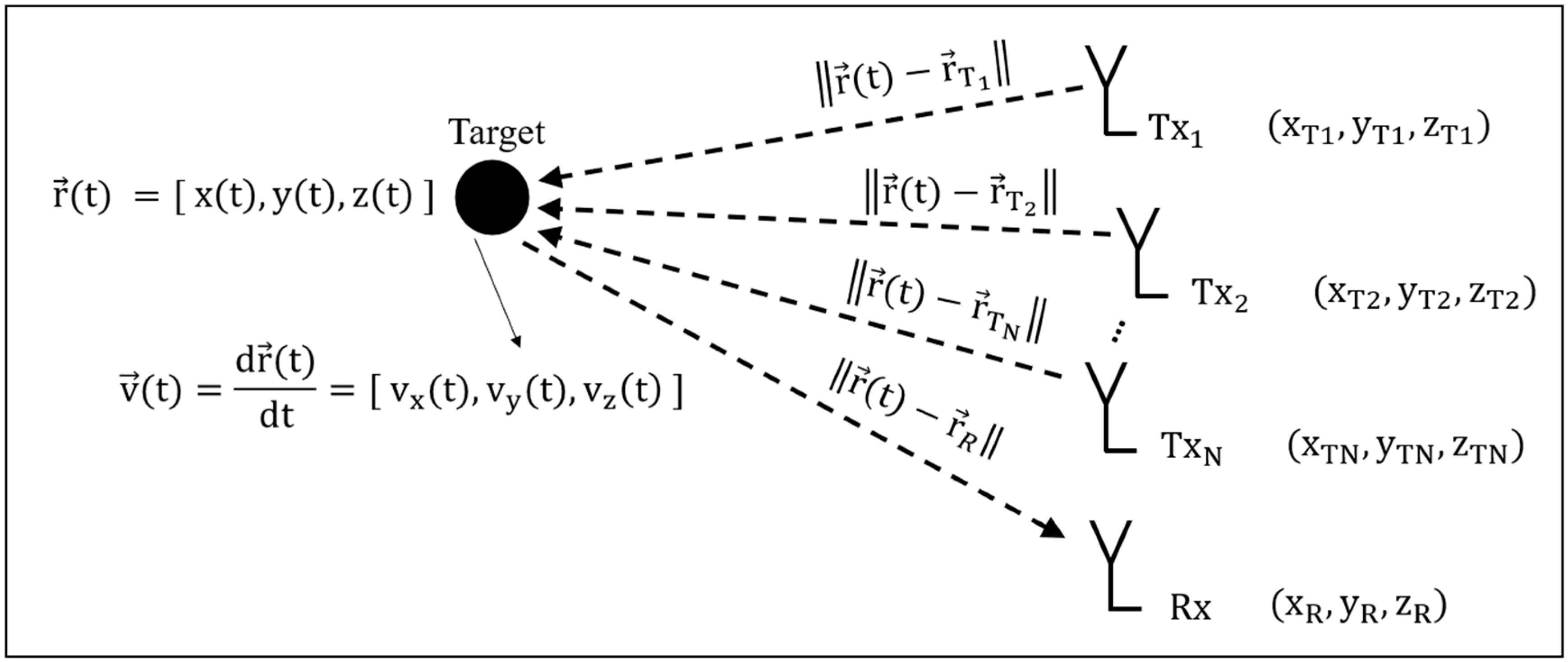
3. Multi Transmitters—Single Receiver MMW Radar

A basic radar, as presented in Figure 1, estimates the velocity component of the target only in the radial direction toward the radar. These data are insufficient for deriving the location of the target. In this study, the possibility of expanding the number of transmitters or the number of receivers is proposed for the creation of multiple velocity components detected by the radar, allowing estimation of target coordinates.

For simplification, the system includes one transmitter and multiple receivers or one receiver and multiple transmitters. Figure 2 shows a system with one receiver and N transmitters.

The utilization of a multi-transmitter system enables the illumination of the target from different directions. The reflected signals are received with different delays, where for each i-th transmitter, the path delay is the summation of the distance from the i-th transmitter to the target and the distance from the target to the receiver, according to the expression:

$${\tau }_{{\mathrm{d}}_{\mathrm{i}}}\left(\mathrm{t}\right)={\displaystyle \frac{1}{\mathrm{c}}}\left[‖\overrightarrow{\mathrm{r}}\left(\mathrm{t}\right)-{\overrightarrow{\mathrm{r}}}_{{\mathrm{T}}_1}‖+‖\overrightarrow{\mathrm{r}}\left(\mathrm{t}\right)-{\overrightarrow{\mathrm{r}}}_{\mathrm{R}}‖\right].$$

(11)

The phase at the received signal that is created by transmitter i is given by

$$\begin{gathered} {\theta }_{\mathrm{i}}\left(\mathrm{t}\right)=2\pi {\mathrm{f}}_0{\tau }_{{\mathrm{d}}_{\mathrm{i}}}\left(\mathrm{t}\right)={\displaystyle \frac{2\pi {\mathrm{f}}_0}{\mathrm{c}}}\left[‖\overrightarrow{\mathrm{r}}\left(\mathrm{t}\right)-{\overrightarrow{\mathrm{r}}}_{{\mathrm{T}}_1}‖+‖\overrightarrow{\mathrm{r}}\left(\mathrm{t}\right)-{\overrightarrow{\mathrm{r}}}_{\mathrm{R}}‖\right]= \\ {\displaystyle \frac{2\pi }{\lambda }}\sqrt{{\left[\mathrm{x}\left(\mathrm{t}\right)-{\mathrm{x}}_{{\mathrm{T}}_{\mathrm{i}}}\right]}^2+{\left[\mathrm{y}\left(\mathrm{t}\right)-{\mathrm{y}}_{{\mathrm{T}}_{\mathrm{i}}}\right]}^2+{\left[\mathrm{z}\left(\mathrm{t}\right)-{\mathrm{z}}_{{\mathrm{T}}_{\mathrm{i}}}\right]}^2}+ \\ {\displaystyle \frac{2\pi }{\lambda }}\sqrt{{\left[\mathrm{x}\left(\mathrm{t}\right)-{\mathrm{x}}_{\mathrm{R}}\right]}^2+{\left[\mathrm{y}\left(\mathrm{t}\right)-{\mathrm{y}}_{\mathrm{R}}\right]}^2+{\left[\mathrm{z}\left(\mathrm{t}\right)-{\mathrm{z}}_{\mathrm{R}}\right]}^2}, \end{gathered}$$

(12)

where $\lambda =\mathrm{c}/{\mathrm{f}}_0$ is the wavelength of the transmission. The output Doppler frequency obtained at the receiver resulting from the i-th transmitter is

$$\begin{gathered} {\mathrm{f}}_{{\mathrm{o}\mathrm{u}\mathrm{t}}_{\mathrm{i}}}\left(\mathrm{t}\right)={\displaystyle \frac{1}{2\pi }}{\displaystyle \frac{\mathrm{d}}{\mathrm{d}\mathrm{t}}}{\theta }_{\mathrm{i}}\left(\mathrm{t}\right)={\displaystyle \frac{1}{\lambda }}{\displaystyle \frac{\left[\mathrm{x}\left(\mathrm{t}\right)-{\mathrm{x}}_{{\mathrm{T}}_{\mathrm{i}}}\right]{\mathrm{v}}_{\mathrm{x}}\left(\mathrm{t}\right)+\left[\mathrm{y}\left(\mathrm{t}\right)-{\mathrm{y}}_{{\mathrm{T}}_{\mathrm{i}}}\right]{\mathrm{v}}_{\mathrm{y}}\left(\mathrm{t}\right)+\left[\mathrm{z}\left(\mathrm{t}\right)-{\mathrm{z}}_{{\mathrm{T}}_{\mathrm{i}}}\right]{\mathrm{v}}_{\mathrm{z}}\left(\mathrm{t}\right)}{\underset{‖\overline{\mathrm{r}\left(\mathrm{t}\right)}-\overline{{\mathrm{r}}_{{\mathrm{T}}_{\mathrm{i}}}}‖}{\underbrace{\sqrt[]{{\left[\mathrm{x}\left(\mathrm{t}\right)-{\mathrm{x}}_{{\mathrm{T}}_{\mathrm{i}}}\right]}^2+{\left[\mathrm{y}\left(\mathrm{t}\right)-{\mathrm{y}}_{{\mathrm{T}}_{\mathrm{i}}}\right]}^2+{\left[\mathrm{z}\left(\mathrm{t}\right)-{\mathrm{z}}_{{\mathrm{T}}_{\mathrm{i}}}\right]}^2}}}}} \\ +{\displaystyle \frac{1}{\lambda }}{\displaystyle \frac{\left[\mathrm{x}\left(\mathrm{t}\right)-{\mathrm{x}}_{\mathrm{R}}\right]{\mathrm{v}}_{\mathrm{x}}\left(\mathrm{t}\right)+\left[\mathrm{y}\left(\mathrm{t}\right)-{\mathrm{y}}_{\mathrm{R}}\right]{\mathrm{v}}_{\mathrm{y}}\left(\mathrm{t}\right)+\left[\mathrm{z}\left(\mathrm{t}\right)-{\mathrm{z}}_{\mathrm{R}}\right]{\mathrm{v}}_{\mathrm{z}}\left(\mathrm{t}\right)}{\underset{‖\overline{\mathrm{r}\left(\mathrm{t}\right)}-\overline{{\mathrm{r}}_{\mathrm{R}}}‖}{\underbrace{\sqrt[]{{\left[\mathrm{x}\left(\mathrm{t}\right)-{\mathrm{x}}_{\mathrm{R}}\right]}^2+{\left[\mathrm{y}\left(\mathrm{t}\right)-{\mathrm{y}}_{\mathrm{R}}\right]}^2+{\left[\mathrm{z}\left(\mathrm{t}\right)-{\mathrm{z}}_{\mathrm{R}}\right]}^2}}}}}. \end{gathered}$$

(13)

The proposed scheme is mainly based on the measurement of frequency deviation due to the Doppler frequency shifts resulting from the target movement. In that sense, only frequency synchronization is required. Constant time delays do not play a role in the Doppler frequency shift obtained at the radar output. Therefore, there is no need to perform phase synchronization between the different transmitted signals.

Equation (13) is composed of a set of equations with three coordinates of the target’s instantaneous location, namely x(t), y(t), and z(t), and three components of the target’s velocity, namely v_x(t), v_y(t), and v_z(t). Solving the set of equations in accordance with the resulting Doppler frequency measurements at the receiver will provide a solution for the spatial velocity and position.

A simple scheme of bi-transmitter Doppler radar used in the experimental setup is shown in Figure 3.

According to the scheme of Figure 3, the coordinates and velocity components of the target are summarized in

Table 1. Parameters for bi-transmitter radar system and target position as in Figure 3.

	X Coordinate	Y Coordinate	Z Coordinate
Target’s location	X(t) = R(t)	$\mathrm{y}\left(\mathrm{t}\right)=0$	$\mathrm{z}\left(\mathrm{t}\right)=0$
Rx location	${\mathrm{x}}_{\mathrm{R}}=0$	${\mathrm{y}}_{\mathrm{R}}=0$	${\mathrm{z}}_{\mathrm{R}}=0$
Tx1 location	${\mathrm{x}}_{{\mathrm{T}}_1}=0$	${\mathrm{y}}_{{\mathrm{T}}_1}=0$	${\mathrm{z}}_{{\mathrm{T}}_1}=0$
Tx2 location	${\mathrm{x}}_{{\mathrm{T}}_2}=0$	${\mathrm{y}}_{{\mathrm{T}}_2}=\mathrm{d}$	${\mathrm{z}}_{{\mathrm{T}}_2}=0$
Target’s velocity	${\mathrm{v}}_{\mathrm{x}}\left(\mathrm{t}\right)$	0	0

.

Introducing the parameters from Table 1 in Equation (13) derives the Doppler frequencies that are produced at the receiver output. Since the scheme involves two transmitters, two frequencies are expected at the receiver output:

$${\mathrm{f}}_{{\mathrm{o}\mathrm{u}\mathrm{t}}_1}\left(\mathrm{t}\right)={\displaystyle \frac{2}{\lambda }}{\mathrm{v}}_{\mathrm{x}}(\mathrm{t}),$$

(14)

$${\mathrm{f}}_{{\mathrm{o}\mathrm{u}\mathrm{t}}_2}\left(\mathrm{t}\right)={\displaystyle \frac{1}{\lambda }}\cdot \left[{\displaystyle \frac{\mathrm{R}\left(\mathrm{t}\right)}{\sqrt{{\mathrm{d}}^2+{\mathrm{R}\left(\mathrm{t}\right)}^2}}}+1\right]\cdot {\mathrm{v}}_{\mathrm{x}}\left(\mathrm{t}\right)=\left[{\displaystyle \frac{\mathrm{R}\left(\mathrm{t}\right)}{\sqrt{{\mathrm{d}}^2+{\mathrm{R}\left(\mathrm{t}\right)}^2}}}+1\right]\cdot {\displaystyle \frac{{\mathrm{f}}_{{\mathrm{o}\mathrm{u}\mathrm{t}}_1}\left(\mathrm{t}\right)}{2}}.$$

(15)

After a few mathematics, the distance R(t) can be separated:

$$\mathrm{R}(\mathrm{t})={\displaystyle \frac{2\frac{{\mathrm{f}}_{{\mathrm{o}\mathrm{u}\mathrm{t}}_2}\left(\mathrm{t}\right)}{{\mathrm{f}}_{{\mathrm{o}\mathrm{u}\mathrm{t}}_1}\left(\mathrm{t}\right)}-1}{\sqrt{1-{\left[2\frac{{\mathrm{f}}_{{\mathrm{o}\mathrm{u}\mathrm{t}}_2}\left(\mathrm{t}\right)}{{\mathrm{f}}_{{\mathrm{o}\mathrm{u}\mathrm{t}}_1}\left(\mathrm{t}\right)}-1\right]}^2}}}\times \mathrm{d}.$$

(16)

It can be seen from Equation (16) that for the measurement of frequencies at the output of a radar system that only measures velocity, additional data can be obtained. In this simplified case, we obtained a measurement of the distance between the target and the radar in addition to the velocity, both of which may be measured over time.

4. Adaptive Processing of a Doppler Signal

In order to track the target position $\mathrm{R}\left(\mathrm{t}\right)$ instantaneously, it is necessary to resolve the two Doppler frequency shifts ${\mathrm{f}}_{{\mathrm{o}\mathrm{u}\mathrm{t}}_1}\left(\mathrm{t}\right)$ and ${\mathrm{f}}_{{\mathrm{o}\mathrm{u}\mathrm{t}}_2}\left(\mathrm{t}\right)$, simultaneously. Noting that these are time-dependent quantities, a time-frequency analysis is required. Surveying the different techniques for spectral analysis, the Short-Time Fourier transform (STFT) was chosen since it enables resolving the two time-varying Doppler shifts ${\mathrm{f}}_{{\mathrm{o}\mathrm{u}\mathrm{t}}_1}\left(\mathrm{t}\right)$ and ${\mathrm{f}}_{{\mathrm{o}\mathrm{u}\mathrm{t}}_2}\left(\mathrm{t}\right)$ at once. Such analysis involves measuring the instantaneous frequency deviations at short time slots. The STFT allows altering the temporal window for optimized processing-time duration, which is crucial for estimating supersonic target velocity and its location. Techniques for spectral analysis, like the Hilbert transform (HT) [24] or Zero-Crossing Rate (ZCR) [25], were examined and excluded from this study because they are mainly fit for measuring a signal with a single frequency (here, two different frequencies are expected).

Other methods, like the Continuous Wavelet Transform (CWT) [26] and Empirical Mode Decomposition (EMD) [27], do not allow varying integration times. Frequency estimation of several different frequencies appearing simultaneously (when an array configuration of multi-transmitters and receivers is used) while optimizing the estimation for each frequency component separately, the STFT was found to be the most suitable and least complex processing technique for analyzing the radar recordings. The adaptive STFT approach, where the temporal window is instantaneously adjusted, was found to be superior compared to other time-frequency processing techniques to resolve variations even in super-sonic target velocity.

Increasing the window temporal width of the STFT improves the velocity measurement resolution. On the other hand, increasing the integration time introduces an overabundance of tracking data regarding the measured target, which is substantial in this study. Extreme caution must be taken when radar measurements are performed on supersonic projectiles. The high velocity of such an evasive target results in ultra-fast location movement. Stretching the STFT window leads to an increase in the probability of missing data or inaccuracies in tracking the target path, especially when the received signal reflected from a supersonic projectile varies faster than the processing time.

The spectral resolution after frequency analysis of the received signal depends on the length T of the time window, which is introduced to the discrete Fourier transform (FFT). The spectral resolution is determined by the frequency broadening due to the effective temporal duration of the STFT window:

$${∆f}_{\mathrm{o}\mathrm{u}\mathrm{t}}^{\mathrm{S}\mathrm{T}\mathrm{F}\mathrm{T}}={\displaystyle \frac{{\mathrm{W}}_{\mathrm{F}}}{\mathrm{T}}}={\displaystyle \frac{{\mathrm{W}}_{\mathrm{F}}}{\mathrm{N}}}{\mathrm{f}}_{\mathrm{s}},$$

(17)

where ${\mathrm{f}}_{\mathrm{s}}$ is the sampling rate of the data, and N is the number of samples within the window duration T. Here, we also consider the window-function factor ${\mathrm{W}}_{\mathrm{F}}$, as summarized in

Table 2. Common window functions and their window function factors.

Window Type	Main Lobe Width	Sidelobe Intensity [dB]	Window Factor
Rectangular	4π/N	−13	2
Triangular	8π/N	−27	4
Hanning	8π/N	−32	4
Hamming	8π/N	−43	4
Blackman	12π/N	−58	6

, for different window shapes. We note that the relationship between ${\mathrm{W}}_{\mathrm{F}}$ and the Main Lobe Width (MLW) is as follows:

$$\mathrm{M}\mathrm{L}\mathrm{W}={\mathrm{W}}_{\mathrm{F}}{\displaystyle \frac{2\pi }{\mathrm{N}}}.$$

(18)

Inspection of Equation (17) reveals an improvement in the spectral resolution as the STFT windowing time T increases. The resulting radial velocity resolution is given by

$${∆\mathrm{v}}_{\mathrm{r}}^{\mathrm{S}\mathrm{T}\mathrm{F}\mathrm{T}}={\displaystyle \frac{\lambda }{2}}{∆f}_{\mathrm{o}\mathrm{u}\mathrm{t}}^{\mathrm{S}\mathrm{T}\mathrm{F}\mathrm{T}}={\displaystyle \frac{\lambda }{2}}\times {\displaystyle \frac{{\mathrm{W}}_{\mathrm{F}}}{\mathrm{N}}}{\mathrm{f}}_{\mathrm{s}}.$$

(19)

For a given sampling rate ${\mathrm{f}}_{\mathrm{s}}$, increasing the number of samples N within the STFT improves the velocity resolution.

During the window duration T, the target velocity varies. In the case of projectiles, the velocity may be reduced because of friction with the air or accelerated because of a supplementary thrust. In the scenario presented in Figure 3, the incremental distance to the target during window duration T can be written as

$$∆\mathrm{R}\left(\mathrm{t},\mathrm{T}\right)=∆\mathrm{R}\left(\mathrm{t}+\mathrm{T}\right)-\mathrm{R}\left(\mathrm{t}\right)={\mathrm{v}}_{\mathrm{r}}\left(\mathrm{t}\right)\times \mathrm{T}+{\displaystyle \frac{1}{2}}{a}_{\mathrm{r}}(\mathrm{t})\times {\mathrm{T}}^2.$$

(20)

where the instantaneous target velocity ${\mathrm{v}}_{\mathrm{r}}(\mathrm{t})$ and acceleration ${\displaystyle \frac{1}{2}}{a}_{\mathrm{r}}(\mathrm{t})$ are given by

$$\begin{gathered} {\mathrm{v}}_{\mathrm{r}}\left(\mathrm{t}\right)={\displaystyle \frac{=∆\mathrm{R}\left(\mathrm{t}+\mathrm{T}\right)-\mathrm{R}\left(\mathrm{t}\right)}{\mathrm{T}}}={\displaystyle \frac{∆\mathrm{R}\left(\mathrm{t}+\mathrm{T}\right)}{\mathrm{T}}}, \\ {a}_{\mathrm{r}}\left(\mathrm{t}\right)={\displaystyle \frac{{\mathrm{v}}_{\mathrm{r}}\left(\mathrm{t}+\mathrm{T}\right)-{\mathrm{v}}_{\mathrm{r}}\left(\mathrm{t}\right)}{\mathrm{T}}}. \end{gathered}$$

(21)

The accumulated phase during the window time T is thus

$$∆\theta (\mathrm{t},\mathrm{T})={\displaystyle \frac{4\pi }{\lambda }}∆\mathrm{R}\left(\mathrm{t},\mathrm{T}\right).$$

(22)

Consequently, the resulting frequency deviation in the Doppler shift is the phase derivative:

$$f_{\mathrm{o}\mathrm{u}\mathrm{t}}\left(\mathrm{t}\right)={\displaystyle \frac{1}{2\pi }}\times {\displaystyle \frac{∆\theta \left(\mathrm{t},\mathrm{T}\right)}{\mathrm{T}}}={\displaystyle \frac{2}{\lambda }}\times {\displaystyle \frac{∆\mathrm{R}\left(\mathrm{t},\mathrm{T}\right)}{\mathrm{T}}}={\displaystyle \frac{2}{\lambda }}{\mathrm{v}}_{\mathrm{r}}\left(\mathrm{t}\right)+\underset{{∆f}_{\mathrm{o}\mathrm{u}\mathrm{t}}^{\mathrm{A}\mathrm{c}\mathrm{c}\mathrm{e}\mathrm{l}\mathrm{e}\mathrm{r}\mathrm{a}\mathrm{t}\mathrm{i}\mathrm{o}\mathrm{n}}}{\underbrace{{\displaystyle \frac{2}{\lambda }}{a}_{\mathrm{r}}(\mathrm{t})\times \mathrm{T}}}.$$

(23)

In the last Equation (23), we find that velocity variation during the temporal STFT duration T creates additional spectral broadening:

$${∆f}_{\mathrm{o}\mathrm{u}\mathrm{t}}^{\mathrm{A}\mathrm{c}\mathrm{c}\mathrm{e}\mathrm{l}\mathrm{e}\mathrm{r}\mathrm{a}\mathrm{t}\mathrm{i}\mathrm{o}\mathrm{n}}(\mathrm{t})={\displaystyle \frac{2}{\lambda }}{a}_{\mathrm{r}}(\mathrm{t})\times \mathrm{T}.$$

(24)

Spectral broadening is a function of the instantaneous radial acceleration ${\mathrm{a}}_{\mathrm{r}}\left(\mathrm{t}\right)$. If the instantaneous target velocity is constant ($a_{\mathrm{r}}\left(\mathrm{t}\right)=0$), no broadening is revealed. The resulting velocity resolution:

$${∆\mathrm{v}}_{\mathrm{r}}^{\mathrm{A}\mathrm{c}\mathrm{c}\mathrm{e}\mathrm{l}\mathrm{e}\mathrm{r}\mathrm{a}\mathrm{t}\mathrm{i}\mathrm{o}\mathrm{n}}={\displaystyle \frac{\lambda }{2}}{∆f}_{\mathrm{o}\mathrm{u}\mathrm{t}}^{\mathrm{A}\mathrm{c}\mathrm{c}\mathrm{e}\mathrm{l}\mathrm{e}\mathrm{r}\mathrm{a}\mathrm{t}\mathrm{i}\mathrm{o}\mathrm{n}}\left(\mathrm{t}\right)=a_{\mathrm{r}}(\mathrm{t})\times \mathrm{T}.$$

(25)

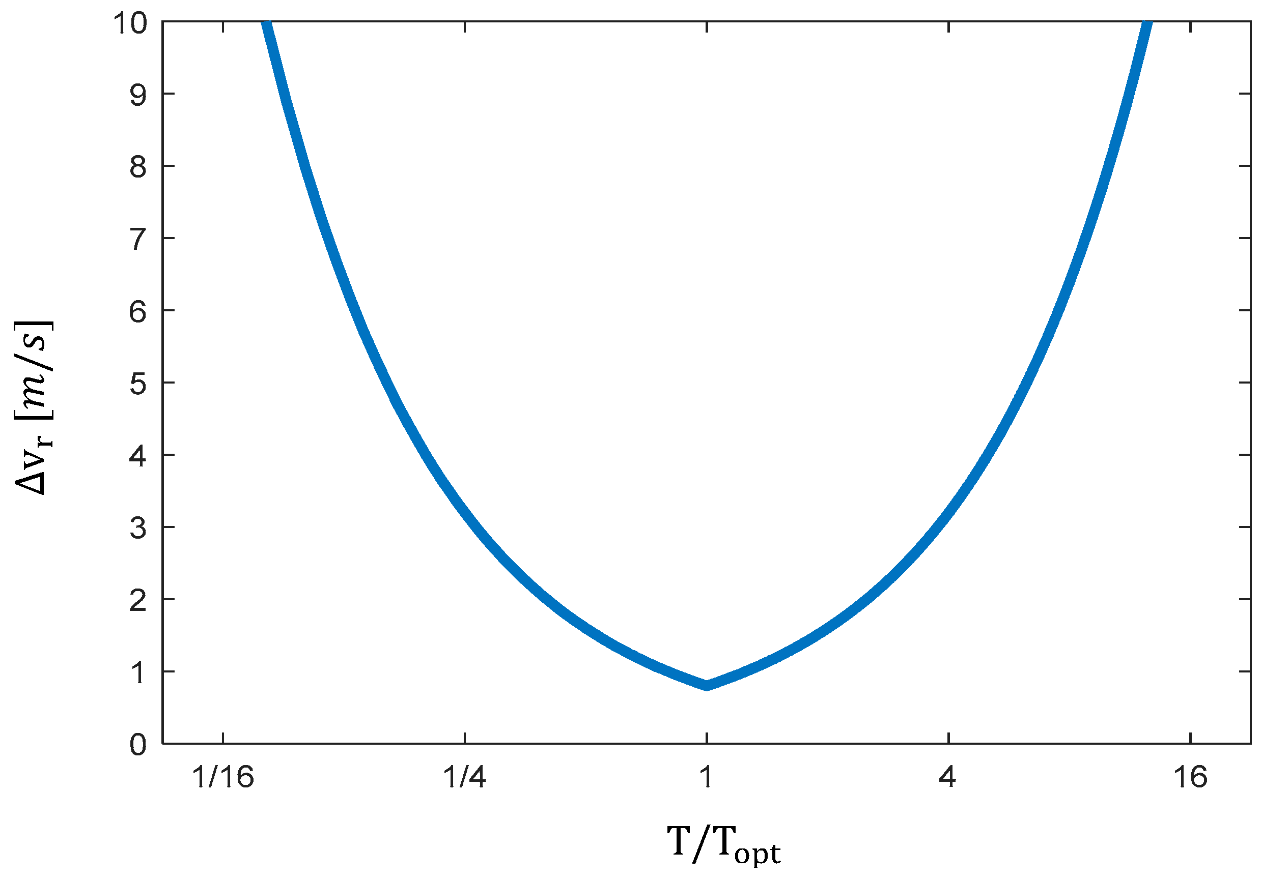
In this case, increasing the STFT window duration T actually leads to a degradation in the velocity resolution. For any time t, there is an optimal value for T for minimum spectral broadening and, thus, for the best velocity resolution:

$${∆f}_{\mathrm{o}\mathrm{u}\mathrm{t}}^{\mathrm{A}\mathrm{c}\mathrm{c}\mathrm{e}\mathrm{l}\mathrm{e}\mathrm{r}\mathrm{a}\mathrm{t}\mathrm{i}\mathrm{o}\mathrm{n}}\left(\mathrm{t}\right)={∆f}_{\mathrm{o}\mathrm{u}\mathrm{t}}^{\mathrm{S}\mathrm{T}\mathrm{F}\mathrm{T}}\to {\displaystyle \frac{2}{\lambda }}{a}_{\mathrm{r}}\left(\mathrm{t}\right)\times \mathrm{T}={\displaystyle \frac{{\mathrm{W}}_{\mathrm{F}}}{\mathrm{T}}}\to {\mathrm{T}}_{\mathrm{o}\mathrm{p}\mathrm{t}}\left(\mathrm{t}\right)=\sqrt{{\displaystyle \frac{2}{\lambda }}\times {\displaystyle \frac{{\mathrm{W}}_{\mathrm{F}}}{a_{\mathrm{r}}\left(\mathrm{t}\right)}}}.$$

(26)

To demonstrate the effect of the temporal window duration T, we calculate the actual velocity resolution:

$$∆{\mathrm{v}}_{\mathrm{r}}=\mathrm{m}\mathrm{a}\mathrm{x}\left\{{\displaystyle \frac{2}{\lambda }}\times {\displaystyle \frac{{\mathrm{W}}_{\mathrm{F}}}{{\mathrm{a}}_{\mathrm{r}}\left(\mathrm{t}\right)}},a_{\mathrm{r}}\left(\mathrm{t}\right)\times \mathrm{T}\right\}.$$

(27)

For the target acceleration, $a_{\mathrm{r}}=100{\displaystyle \frac{\mathrm{m}}{{\mathrm{s}}^2}}$, as shown in Figure 4. The carrier frequency is set to $f_0=100\mathrm{G}\mathrm{H}\mathrm{z}$ ($\lambda =3\mathrm{m}\mathrm{m}$). The minimum $∆{\mathrm{v}}_{\mathrm{r}}$ is obtained at $\mathrm{T}={\mathrm{T}}_{\mathrm{o}\mathrm{p}\mathrm{t}}$.

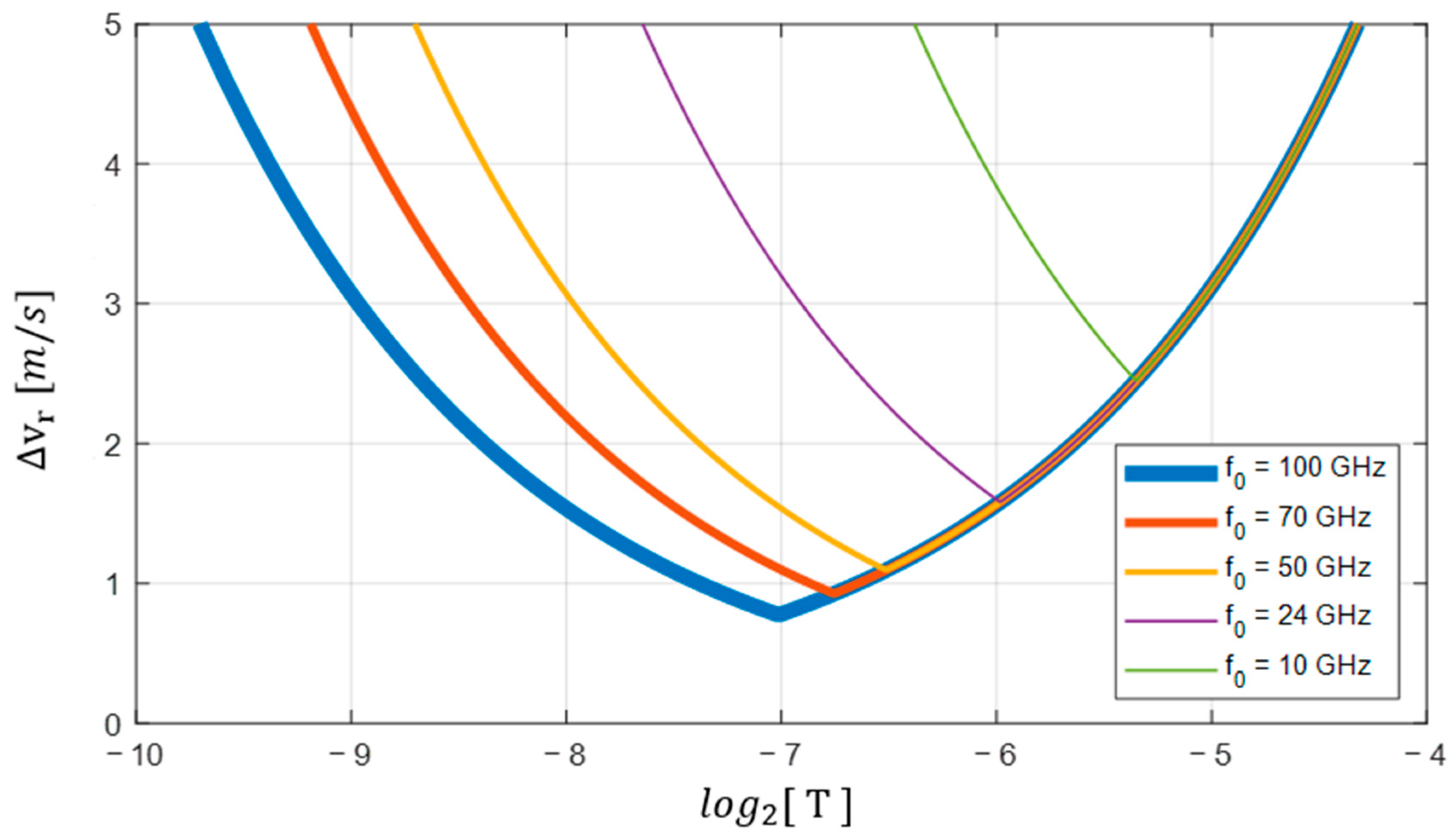
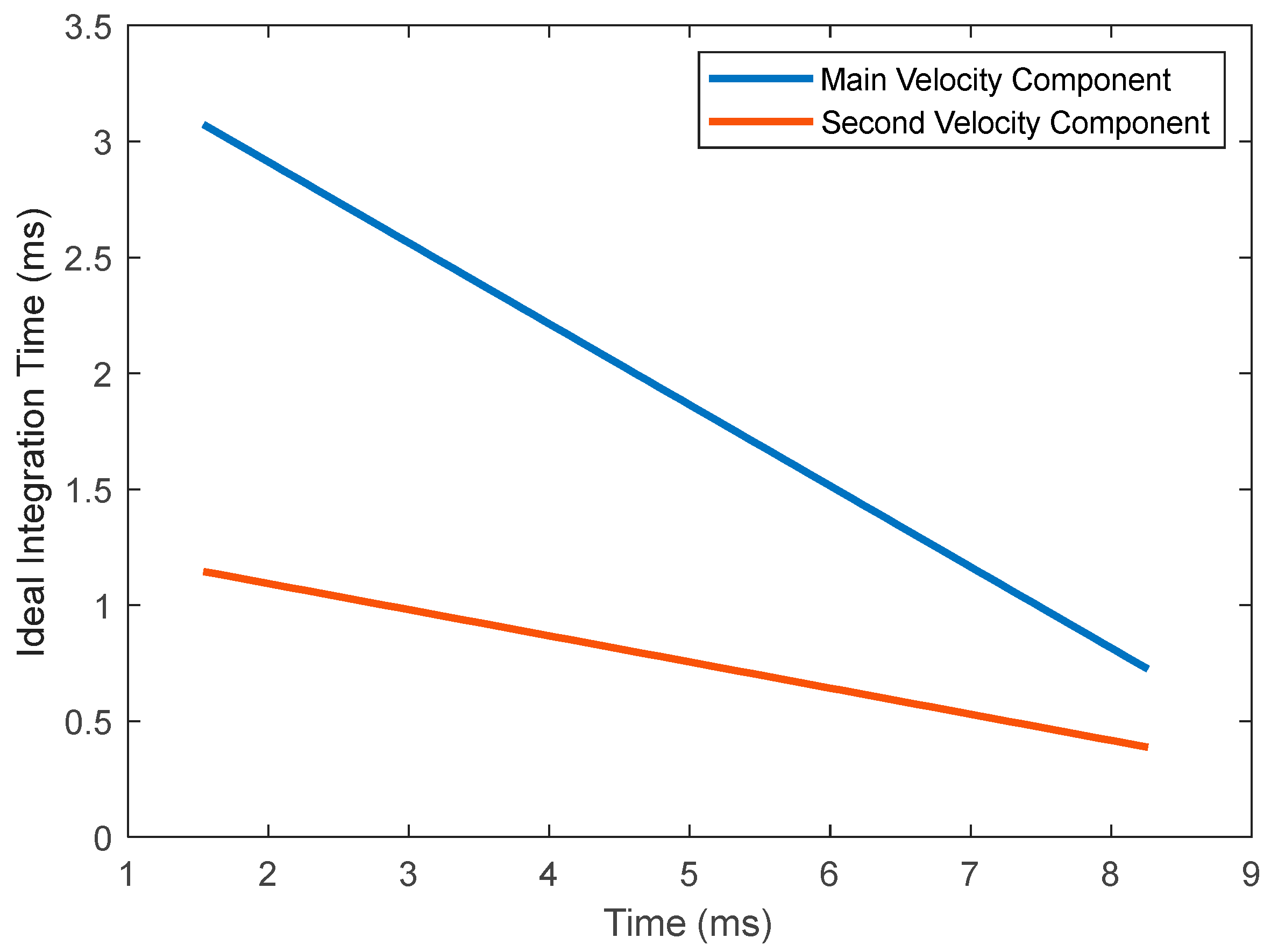
Note that the optimal integration time ${\mathrm{T}}_{\mathrm{o}\mathrm{p}\mathrm{t}}$ is dependent on the transmission frequency $f_0$. Utilization of a higher frequency results in better resolution. The graphs in Figure 5 present the actual velocity resolution $∆{\mathrm{v}}_{\mathrm{r}}$ as a function of the integration time T for a moving target with the same acceleration $a_{\mathrm{r}}=100{\displaystyle \frac{\mathrm{m}}{{\mathrm{s}}^2}}$.

The target velocity variations during flight (expressed by the instantaneous acceleration $a_{\mathrm{r}}\left(t\right)$) require adaptive adjustment of the STFT integration time during tracking, as shown in Algorithm 1.

Algorithm 1. Adaptive STFT for high-variant velocity targets.

$\mathrm{Inputs}:\mathrm{x}\left(\mathrm{t}\right)—\mathrm{raw}\mathrm{signal}\mathrm{from}\mathrm{a}\mathrm{Doppler}\mathrm{radar}\mathrm{over}\mathrm{a}\mathrm{time}\mathrm{of}{\mathrm{T}}_{\mathrm{s}\mathrm{i}\mathrm{g}\mathrm{n}\mathrm{a}\mathrm{l}}$. $\hspace{1em}\hspace{1em}\hspace{1em}\hspace{1em}\hspace{1em}\hspace{1em}\lambda$—wavelength of transmission. $\hspace{1em}\hspace{1em}\hspace{1em}\hspace{1em}\hspace{1em}\hspace{1em}{a}_{\mathrm{m}\mathrm{a}\mathrm{x}}$—maximum expected acceleration. $\hspace{1em}\hspace{1em}\hspace{1em}\hspace{1em}\hspace{1em}\hspace{1em}{O}_{\mathrm{f}}$—time overlap factor. Output: ${\mathrm{v}}_{\mathrm{d}}\left[i\right]$—Doppler velocity after STFT optimization. Initiations: $a_{\mathrm{r}}$ = $a_{\mathrm{m}\mathrm{a}\mathrm{x}}$. $\hspace{1em}\hspace{1em}\hspace{1em}\hspace{1em}\hspace{1em}\hspace{1em}{\mathrm{T}}_{\mathrm{o}\mathrm{p}\mathrm{t}}=\sqrt{{\displaystyle \frac{2}{\lambda }}\times {\displaystyle \frac{{\mathrm{W}}_{\mathrm{F}}}{a_{\mathrm{r}}}}}$—Equation (26). $\hspace{1em}\hspace{1em}\hspace{1em}\hspace{1em}\hspace{1em}\hspace{1em}{\mathrm{x}}_{\mathrm{T}}\left(\mathrm{t}\right)=\mathrm{x}(0:{\mathrm{T}}_{\mathrm{o}\mathrm{p}\mathrm{t}})$$—\mathrm{collect}\mathrm{samples}\mathrm{according}\mathrm{to}{\mathrm{T}}_{\mathrm{o}\mathrm{p}\mathrm{t}}$. $\hspace{1em}\hspace{1em}\hspace{1em}\hspace{1em}\hspace{1em}\hspace{1em}{\mathrm{X}}_{\mathrm{T}}\left(\mathrm{f}\right)=\mathrm{F}\mathrm{F}\mathrm{T}\left\{{\mathrm{x}}_{\mathrm{T}}\left(\mathrm{t}\right)\right\}$$—\mathrm{calculate}\mathrm{the}\mathrm{FFT}\mathrm{over}\mathrm{time}{\mathrm{T}}_{\mathrm{o}\mathrm{p}\mathrm{t}}$. $\hspace{1em}\hspace{1em}\hspace{1em}\hspace{1em}\hspace{1em}\hspace{1em}{f}_{\mathrm{d}}={arg}_{max}\left\{{\mathrm{X}}_{\mathrm{T}}\left(\mathrm{f}\right)\right\}$—find the frequency with the highest energy. $\hspace{1em}\hspace{1em}\hspace{1em}\hspace{1em}\hspace{1em}\hspace{1em}{\mathrm{v}}_{\mathrm{d}}\left[i\right]={\displaystyle \frac{\lambda }{2}}{f}_{\mathrm{d}}$—compute the velocity according to Equation (9). $\hspace{1em}\hspace{1em}\hspace{1em}\hspace{1em}\hspace{1em}\hspace{1em}\mathrm{t}={\mathrm{T}}_{\mathrm{o}\mathrm{p}\mathrm{t}}$$—\mathrm{start}\mathrm{the}\mathrm{loop}\mathrm{after}\mathrm{the}\mathrm{first}{\mathrm{T}}_{\mathrm{o}\mathrm{p}\mathrm{t}}$ samples. while (t < ${\mathrm{T}}_{\mathrm{s}\mathrm{i}\mathrm{g}\mathrm{n}\mathrm{a}\mathrm{l}}$) $\hspace{1em}\hspace{1em}\hspace{1em}\hspace{1em}\hspace{1em}\hspace{1em}i=i+1$ $\hspace{1em}\hspace{1em}\hspace{1em}\hspace{1em}\hspace{1em}\hspace{1em}{\mathrm{T}}_{\mathrm{o}\mathrm{p}\mathrm{t}}=\sqrt{{\displaystyle \frac{2}{\lambda }}\times {\displaystyle \frac{{\mathrm{W}}_{\mathrm{F}}}{a_{\mathrm{r}}}}}$$—\mathrm{Equation}\left(26\right)(a_{\mathrm{r}}$$=a_{\mathrm{m}\mathrm{a}\mathrm{x}}$ in the first iteration). $\hspace{1em}\hspace{1em}\hspace{1em}\hspace{1em}\hspace{1em}\hspace{1em}{\mathrm{x}}_{\mathrm{T}}\left(\mathrm{t}\right)=\mathrm{x}(\mathrm{t}:\mathrm{t}+{\mathrm{T}}_{\mathrm{o}\mathrm{p}\mathrm{t}})$$—\mathrm{collect}\mathrm{samples}\mathrm{over}\mathrm{time}{\mathrm{T}}_{\mathrm{o}\mathrm{p}\mathrm{t}}$ after time t. $\hspace{1em}\hspace{1em}\hspace{1em}\hspace{1em}\hspace{1em}\hspace{1em}{\mathrm{X}}_{\mathrm{T}}\left(\mathrm{f}\right)=\mathrm{F}\mathrm{F}\mathrm{T}\left\{{\mathrm{x}}_{\mathrm{T}}\left(\mathrm{t}\right)\right\}$—calculate the FFT over time T. $\hspace{1em}\hspace{1em}\hspace{1em}\hspace{1em}\hspace{1em}\hspace{1em}{f}_{\mathrm{d}}={arg}_{max}\left\{{\mathrm{X}}_{\mathrm{T}}\left(\mathrm{f}\right)\right\}$—find the frequency with the highest energy. $\hspace{1em}\hspace{1em}\hspace{1em}\hspace{1em}\hspace{1em}\hspace{1em}{\mathrm{v}}_{\mathrm{d}}[i]={\displaystyle \frac{\lambda }{2}}{f}_{\mathrm{d}}$—compute the velocity according to Equation (9). $\hspace{1em}\hspace{1em}\hspace{1em}\hspace{1em}\hspace{1em}\hspace{1em}{a}_{\mathrm{r}}={\displaystyle \frac{{\mathrm{v}}_{\mathrm{d}}\left[i\right]-{\mathrm{v}}_{\mathrm{d}}[i-1]}{{\mathrm{T}}_{\mathrm{o}\mathrm{p}\mathrm{t}}}}$—calculate acceleration for the next iteration. $\hspace{1em}\hspace{1em}\hspace{1em}\hspace{1em}\hspace{1em}\hspace{1em}t=t+O_{\mathrm{f}}\times {\mathrm{T}}_{\mathrm{o}\mathrm{p}\mathrm{t}}$—promote time index for the next iteration. end

In addition to the identification of the optimal integration time, the distinct advantages of transmitting high frequencies in the MMW regime are revealed. Extremely high frequencies allow higher resolution in speed estimation, even with a shorter integration time. Doubling the transmission frequency allows the integration time to decrease by a factor of $\sqrt{2}$.

$$if{f}_2=2\times f_1:{\displaystyle \frac{{\mathrm{T}}_1}{{\mathrm{T}}_2}}={\displaystyle \frac{\sqrt{\frac{{\mathrm{W}}_{\mathrm{F}}}{\mathrm{a}}\times \frac{\mathrm{c}}{2{\mathrm{f}}_1}}}{\sqrt{\frac{{\mathrm{W}}_{\mathrm{F}}}{\mathrm{a}}\times \frac{\mathrm{c}}{2{\mathrm{f}}_2}}}}=\sqrt{{\displaystyle \frac{{\mathrm{f}}_2}{{\mathrm{f}}_1}}}=\sqrt{2},$$

(28)

where ${\mathrm{T}}_1$ is the optimized integration time for acceleration while transmitting ${\mathrm{f}}_1$ and where ${\mathrm{T}}_2$ is the optimized integration time for the same acceleration while transmitting ${\mathrm{f}}_2$. The difference between the integration times is as follows:

$${\mathrm{T}}_2={\displaystyle \frac{{\mathrm{T}}_1}{\sqrt{2}}}$$

(29)

This means that when a higher frequency ${\mathrm{f}}_2$ is used, the integration time ${\mathrm{T}}_2$ is shorter. Reducing the integration time allows the estimation of velocity in shorter time windows and, therefore, enables more continuous tracking of the measured target.

5. Experiments in a Shooting Range

The proposed method in this paper was tested at a shooting range when the target of the radar is a metal bullet. The model was tested in its abstract form for extra clarification, presentation of the strength of the correctness of the proposed model, and facilitating the processing of the data from the radar.

The radar system was placed close to the expected point of impact of the bullet, as close as possible to the expected trajectory of the projectile, and remained safe without any damage. The radar system included one receiver and two transmitters, with the receiver adjacent to the first transmitter and the second transmitter placed at a distance d from the receiver and the first transmitter, as shown in Figure 6.

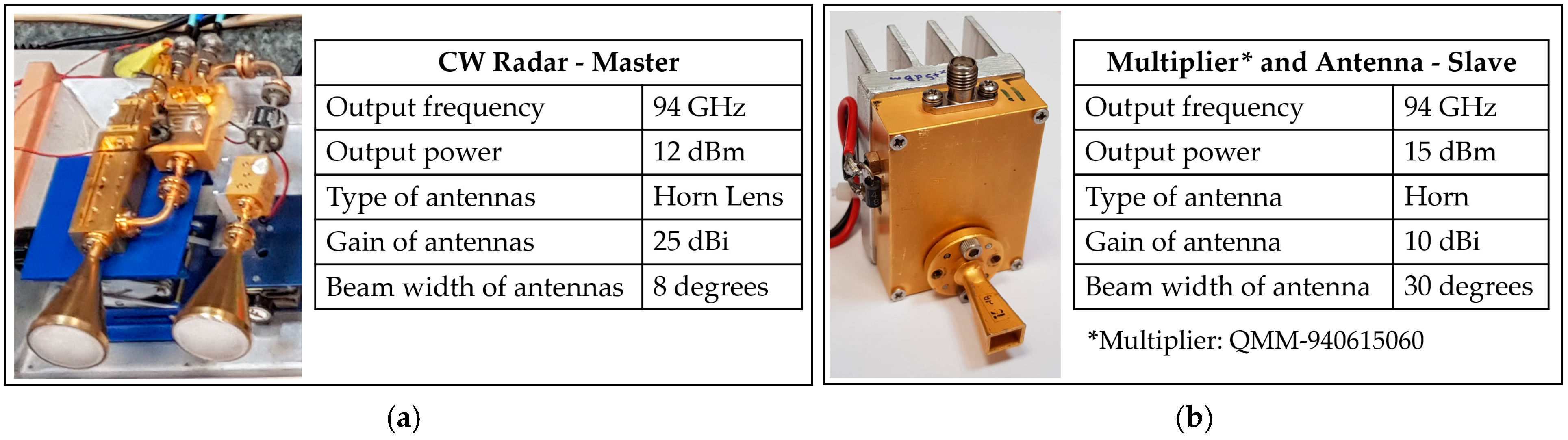
The radar system used in the experiment consists of a master unit and slave unit, as presented in Figure 7.

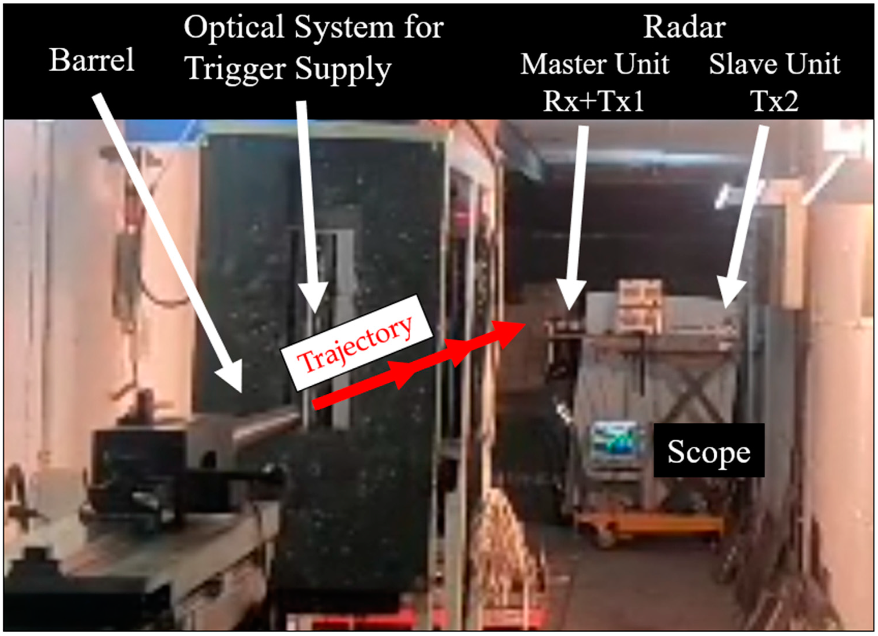
The output of the radar is analog and was recorded by a scope. The scope was programmed so that it performed a cyclical recording until 60 ms after receiving an external trigger. The external trigger is an optical system output that detects a bullet passing through it and provides data regarding the velocity of the bullet while passing through it. The cyclic recording of the scope is a total of 100 ms, where the data saved at the moment of receiving the trigger are 40 ms before the bullet passes in the optical system and 60 ms after the bullet passes through the optical system.

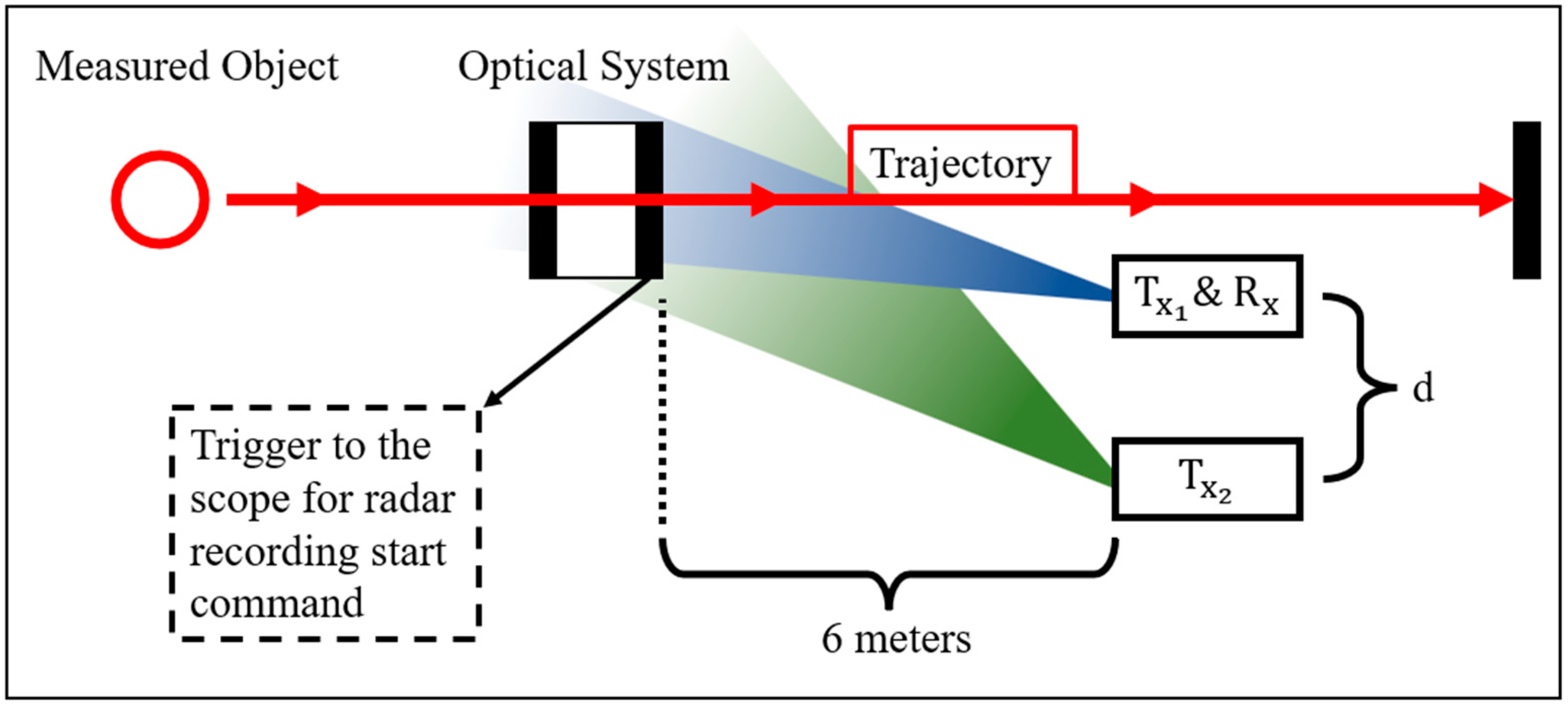
A diagram of the locations of the systems in the shooting range is shown in Figure 8. Importantly, the distance between the optical system that provides a trigger and the radar is exactly 6 m. This distance will help validate the correctness of the measurement and calculations.

The selection of the different locations and resulting distances in Figure 8 has a high influence on the obtained resolution of the range estimation. The presented layout of the radar placement was chosen in accordance with the limited space in the shooting gallery where the experiment was carried out. 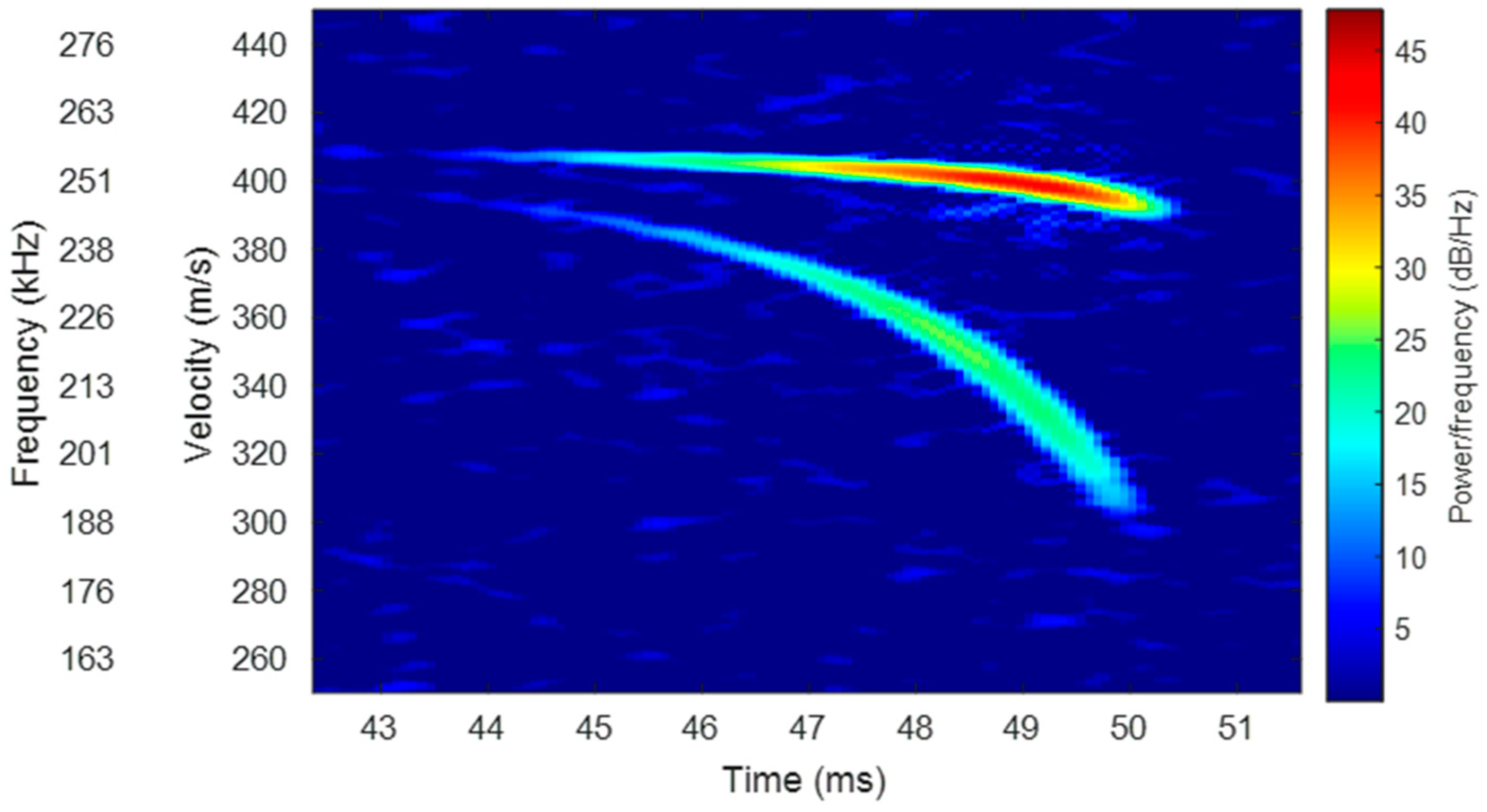The selection of distance d in Figure 8 has a high influence on the obtained resolution of the range estimation (see [20]). The shooting was recorded by the radar and the scope; as expected, two frequencies were received at the radar output. These frequencies change in time, depending on the relative velocity and the relative position of the bullet in relation to the radar. To present the data from the radar, which is represented in frequencies over time, the radar recording is shown after performing STFT, as introduced in Figure 9.

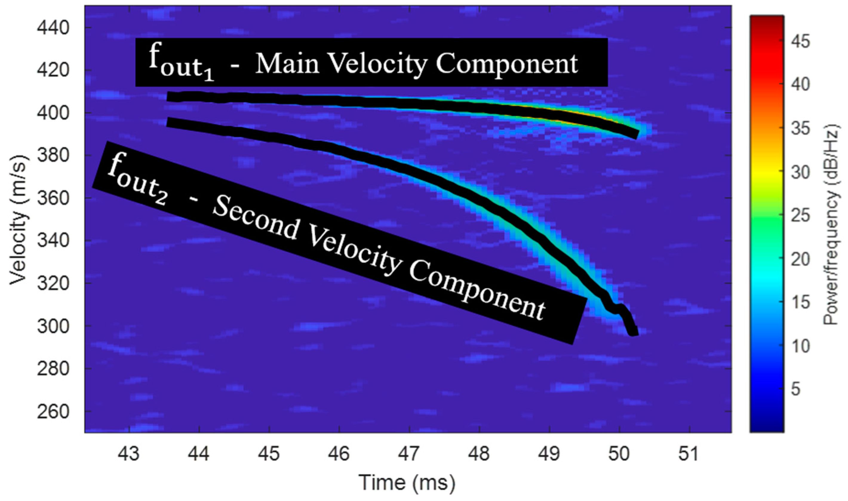
The calculations proposed in this paper require velocity vectors to be extracted from the data recorded from the radar. The spectrogram graph from Figure 9 was taken to extract two velocity component vectors, and the extraction result can be seen in Figure 10.

Figure 10 shows the extraction of data for two velocity components at any given measurement time. The data are extracted by following frequencies that have the maximum energy from the spectrogram graph at every time slot. The spectrogram graph in Figure 10 is not ideal for every possible acceleration of the target, and it can even be seen that at each point in time, there is a different acceleration, and there are different accelerations for each velocity component. To extract the data accurately from the spectrogram, we can use Equation (26), which shows a way to choose an appropriate integration time for each acceleration at each time slot. The vectors from Figure 10 were entered into the calculation of acceleration as a differential and then entered into Equation (26) to find the appropriate integration time for each time slot. The calculated integration times for each velocity component over time are shown in Figure 11.

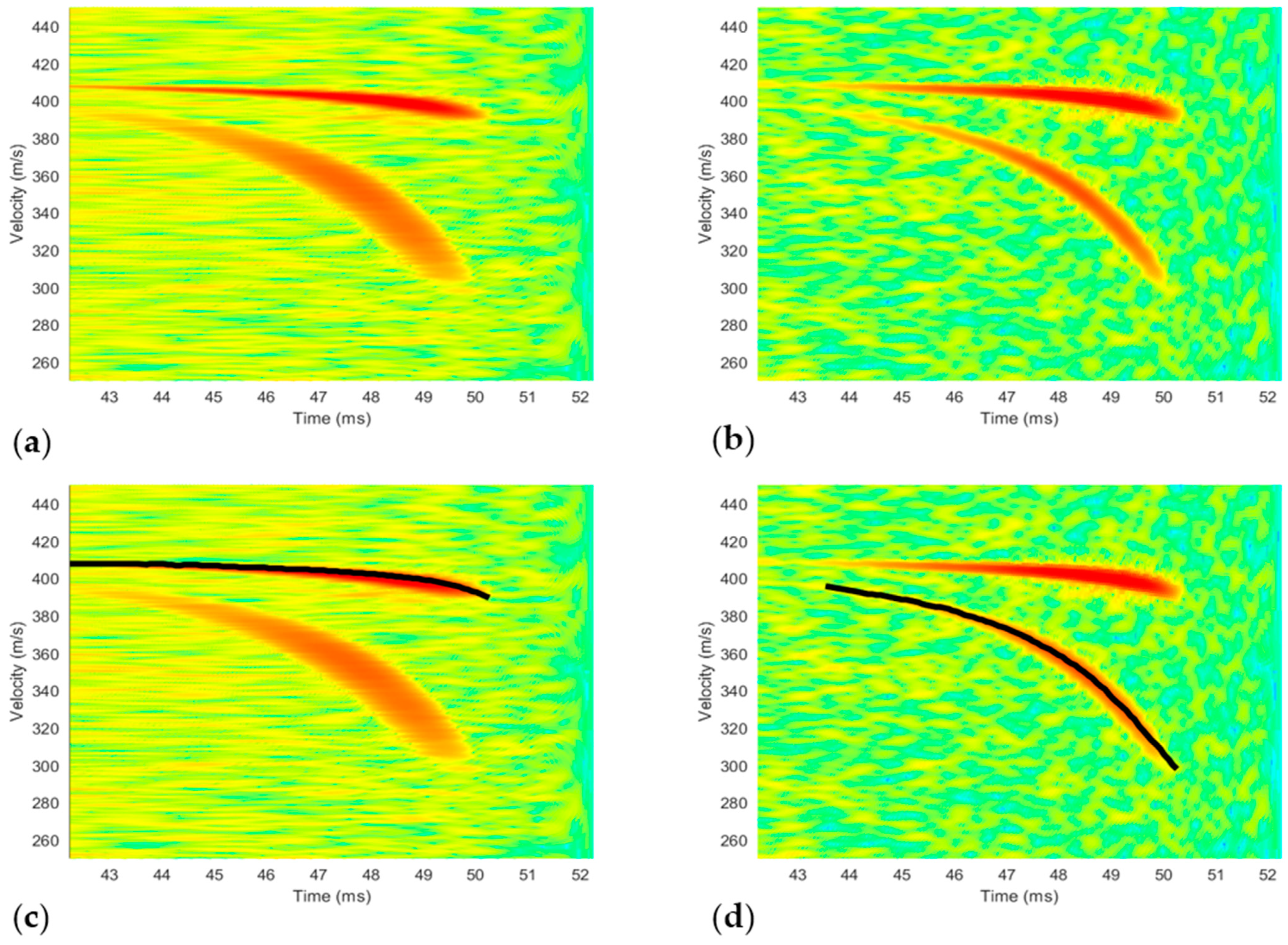
The integration times were taken for an optimized calculation of the velocity components via Algorithm 1. Two different spectrogram graphs were created, one for each velocity component separately, to perform an optimization for each component separately. The spectrograms and extraction of the velocity vectors are shown in Figure 12.

Optimization for the first velocity component improves it over time so that it is possible to obtain more accurate information and even obtain information about the measured target at an earlier time than was shown in the spectrogram without optimization in Figure 10. While the optimization is being performed for the first velocity component, the second velocity component receives less attention and is not displayed properly. The second situation, where the optimization is performed for the second velocity component so that the spectrogram is of better quality with more accurate information, while the first velocity component is less well represented, can also be observed. It can be concluded that optimization for the integration time for each velocity component separately yields the most accurate results over time given an initial calculation of acceleration, even if it is calculated imprecisely.

The velocity vectors, which were extracted according to the process presented in Figure 12, were inserted into Equation (16) to calculate the distance between the target and the radar. Owing to the transmission power limitations of the system, the distance of the target detection is limited, and no data regarding the target were found in the first 4 ms after receiving the trigger from the optical system in the shooting range. To calculate the trajectory from the moment of receiving the trigger, a linear line was extrapolated to estimate the distance according to the radar from the first moment of the trigger. The result of the distance calculation from the radar measurements plus the distance estimated from the moment of receiving the trigger at 40 ms is shown in Figure 13.

The estimated distance was calculated from 44 ms back to 40 ms. The estimated distance at the time of receiving the trigger is exactly 6 m. Six meters is the exact distance between the radar and the optical system, which gives the trigger, as shown in Figure 8. The radar measurement produced a correct result that corresponds to the dimensions of the range.

6. Discussion

A technique for tracking evasive targets is presented, using multi-static continuous wave (CW) radars operating in the millimeter wave regime. The concept is analyzed theoretically and verified experimentally in a shooting range. We demonstrate tracking a single target (a bullet) using multiple CW transmissions. The radial target velocity is estimated via the respective Doppler frequency shifts obtained at the receiver. The presented technique enables the calculation of the instantaneous target location. The time-frequency signal processing enables tracking even for a super-sonic moving target. Experiments in a shooting gallery demonstrate the applicability of the proposed technique for small RCS targets. Utilization of multiple transmissions is suitable for tracking several targets; moving within the field of view of the receiver, however, may require massive data processing and analysis. The maximum range for tracking targets is mainly limited by the spatial covering of the MIMO radar array, while the detection and tracking performances for each target are limited by its corresponding received signal-to-noise ratio.

This study presents range estimation via velocity measurement using multi-site Doppler radar. The velocity measurement is based on identifying the Doppler frequency shifts resulting from the target scattering toward the different receivers. The maximum velocity for measurement is affected by the frequency response at the baseband and the sampling rate of the following digitizer. We note that the component with the narrowest bandwidth in the RF chain is the W-band down conversion mixer with a bandwidth of 1 GHz. This bandwidth enables tracking of super-sonic moving targets. The analysis shows that the main limitation of the tracking resolution is the acceleration dynamics of the target. The study reveals an optimized procedure that utilized an adaptive integration time for attaining high resolution even for fast varying target velocities.

Since the target tracking is based on a Doppler frequency shift determined by its velocity, static targets are ignored. Thus, unlike common radar systems that measure range directly, the proposed scheme exhibits built-in immunity against clutter caused by stationary objects. In the common range-Doppler radar systems, the static targets can be subtracted to some extent only after processing the data. In addition, in such radar systems with direct range estimation, the static targets determine the dynamic range of the detection power, which significantly lowers the detection probability of targets with low RCS, while the proposed MIMO radar scheme is able to detect very small objects, as demonstrated here.

In this study, an analysis was performed on a multi-site radar for the detection and tracking of a fast-moving, low-RCS target. An adaptive signal processing technique is developed for tracking the position of a super-sonic target along its path of flight. The detection scheme was demonstrated in a controlled experiment in a shooting range, and the capabilities of tracking a projectile were confirmed experimentally. Following research efforts will be directed to the detection and tracking of multiple objects using MIMO radar configuration, as shown in Figure 2.

7. Conclusions

The range measurement method proposed in this article was found to be particularly reliable in a noisy environment and superior in the tracking of particularly fast and stealthy targets. The use of the CW radar yielded the detection of only the target without clutter in space, a high SNR compared with wide bandwidth methods, and velocity and range resolution without a model limit. The use of the millimeter wave regime yielded high-quality tracking of small targets and a reduction in processing time compared with the use of lower frequencies, resulting in shorter detection times and the ability to detect targets with high acceleration. An optimization method was presented to adaptively optimize the processing times as a function of the target’s instantaneous acceleration, and high optimization was achieved in the estimation of the target’s range in continuous tracking. Compared with existing systems for range measurement, the method that was proposed and tested in projectile firing experiments achieved high performance in terms of range resolution while using a cheap radar system.