Noise Radar Waveform Design Using Evolutionary Algorithms and Negentropy Constraint

Abstract

In recent years, several advantages of noise radars have positioned this technology as a promising alternative to conventional radar technology. Immunity to jamming, low mutual interference, and low probability of interception are good examples of these advantages. However, the nature of random sequences introduces several issues, such as fluctuations in the range sidelobes of the autocorrelation function causing high sidelobe levels, hence not exploitable by radar systems. This study introduces the use of multi-objective evolutionary (MOE) algorithms to design noise radar waveforms with good autocorrelation properties as well as a low peak-to-average power ratio (PAPR). A set of Pareto-optimal waveforms are produced and, most importantly, entropy is introduced as a constraint in order to maintain the transmitted signal close to a full non-deterministic waveform. Moreover, a relation between PAPR and negentropy (negative entropy) is established theoretically and validated with other authors’ simulations.

1. Introduction

Noise radar technology (NRT) differs from conventional radars in that it uses non-deterministic waveforms. To maximize signal-to-noise ratio (SNR), the process of estimating the range and velocity of the illuminated target is done by matched filtering, that is, correlating the transmitted and received signals both in the time and Doppler domains. However, implementing this “correlation receiver” in real time is computationally heavy, which explains why, although this idea dates back to the middle of the last century [1], NRT was only revisited at the beginning of this century [2,3,4].

Low-probability-of-intercept (LPI) radar systems have been emerging in recent years, and NRT is a viable option in this field. Traditionally, by analyzing conventional radar systems in the frequency domain over a long period, it is possible to detect if a signal is present or not by deciding upon a threshold value. Having continuous wave (CW) non-deterministic coded waveforms in a wide band minimizes this issue and makes intercepting these systems a challenging task [5]. Despite State-of-the-Art electronic support measures (ESM) systems being able to implement time–frequency analysis, non-deterministic waveforms have the desired spectral shape and are very challenging to classify using this approach.

In addition, the unique characteristics of noise radar waveforms can contribute to the effectiveness of sensor fusion systems. By leveraging non-deterministic waveforms, noise radar can operate efficiently even in environments with high mutual interference. This ensures that data from multiple sensors can be integrated more seamlessly, enhancing the overall accuracy and reliability of the sensor network. The inherent LPI and high immunity to jamming of noise radar systems further support robust and secure sensor fusion, making them a valuable component in complex detection and tracking scenarios.

Noise radar systems have other already demonstrated advantages over conventional deterministic systems [5,6]:

• Low mutual interference (MI): when different radars coexist in a limited environment and frequency band, interference among them may occur. In NRT, this is mitigated due to each radar perceiving the others’ signals as noise [7];
• High immunity to jamming: noise radar waveforms are harder to identify. Since jamming can be made by creating deceptive false targets or injecting a signal to cancel the transmitted one, there is a need to know the transmitted waveform. This is harder to achieve if there are no signal libraries available or the transmitted signal is (or looks) random.

Nevertheless, NRT present several challenges, particularly in designing an exploitable waveform, since the generated Gaussian noise signal to be transmitted has an undesired characteristic: the high level of the autocorrelation function (ACF) sidelobes. Reducing the sidelobe level of the ACF typically results in a high peak to average power ratio (PAPR), which is a metric that represents the peak power divided by the average power (see Equation (3)). Addressing this challenge, this paper aims to create a method to find a good compromise between a waveform with favorable correlation properties and maintaining a low PAPR, while introducing the use of negentropy (negative entropy) to keep the synthesized signal close to a Gaussian distribution, therefore enhancing its theoretical LPI characteristics. Furthermore, a relation between negentropy and PAPR is established.

We formulate a multi-objective optimization problem (MOP) which we addressed by proposing an algorithm based on the NSGA-II [8] family. Also, a constraint based on entropy is studied and used to control the “randomness” of the resulting waveform.

This paper is organized as follows: in the Introduction, noise radar systems’ advantages and drawbacks are presented, while giving an overview on the objectives of the paper. Section 2 presents the challenges of designing a noise radar waveform, surveys recently published techniques to tackle this issue, and reviews methods commonly used to classify a LPI radar. In the following section, the MOP is formulated, while Section 4 describes the approach proposed to address it. In Section 5, experimental results are reported, concluding the paper in Section 6 with summary remarks and guidelines for future work.

2. Design and Challenges of Noise Radar Waveforms

This section explores the main challenges of noise radar waveform design, how the LPI characteristics of the signal can be measured, and what insights can be extracted from these observations.

2.1. Noise Radar Waveforms and Challenges

It is important to clarify what we mean by non-deterministic waveforms, since LPI and other properties of NRT rely on the randomness or unpredictability of the signal.

Deterministic machines are intrinsically incapable of generating pure random signals. Hence, in principle, NRT waveforms should derive from physical factors such as thermal noise. However, the use of these analog noise sources becomes impractical since they present several constraints in resolution and dynamic range [9]. Therefore, digitally generated signals are preferred by implementing pseudorandom number-generators (PRNG) optimized to the specific application.

Nevertheless, all the advantages of NRT come with a cost. The design of waveforms based on PRNG (such as a Gaussian noise) faces two main issues, which are described next.

• The ACF is a fundamental concept when designing radar waveforms, specifically because it permits the performance analysis of the correlation receiver—the preferred method to estimate target position and velocity [10]. The ACF measures the similarity between a signal $x\left[n\right]$ and a delayed version thereof as a function of the delay:

  $$R\left(m\right)=\sum _{n=0}^{N-1}x\left[n\right]x[n-m],$$

  (1)

  where m is the delay and N is the total number of samples. A non-deterministic signal has unpredictable variations in amplitude and phase, which contributes to fluctuations in the ACF, influencing its behavior and shape. Therefore, it is essential to implement sidelobe suppression techniques for enhancing the overall performance and reliability of radar systems. Moreover, peak-to-sidelobe level (PSL) is usually used as a metric to define the ratio of the amplitude of the main lobe to the amplitude of the highest sidelobe of the ACF. In NRT, the PSL can be estimated as:

  $${\mathrm{PSL}}_{\mathrm{dB}}=-10{log}_{10}\left(BT\right)+K,$$

  (2)

  where B is the bandwidth, T is the waveforms’ time duration and K is a constant depending on the PRNG distribution usually taking values between 10 and 12 dB [9].
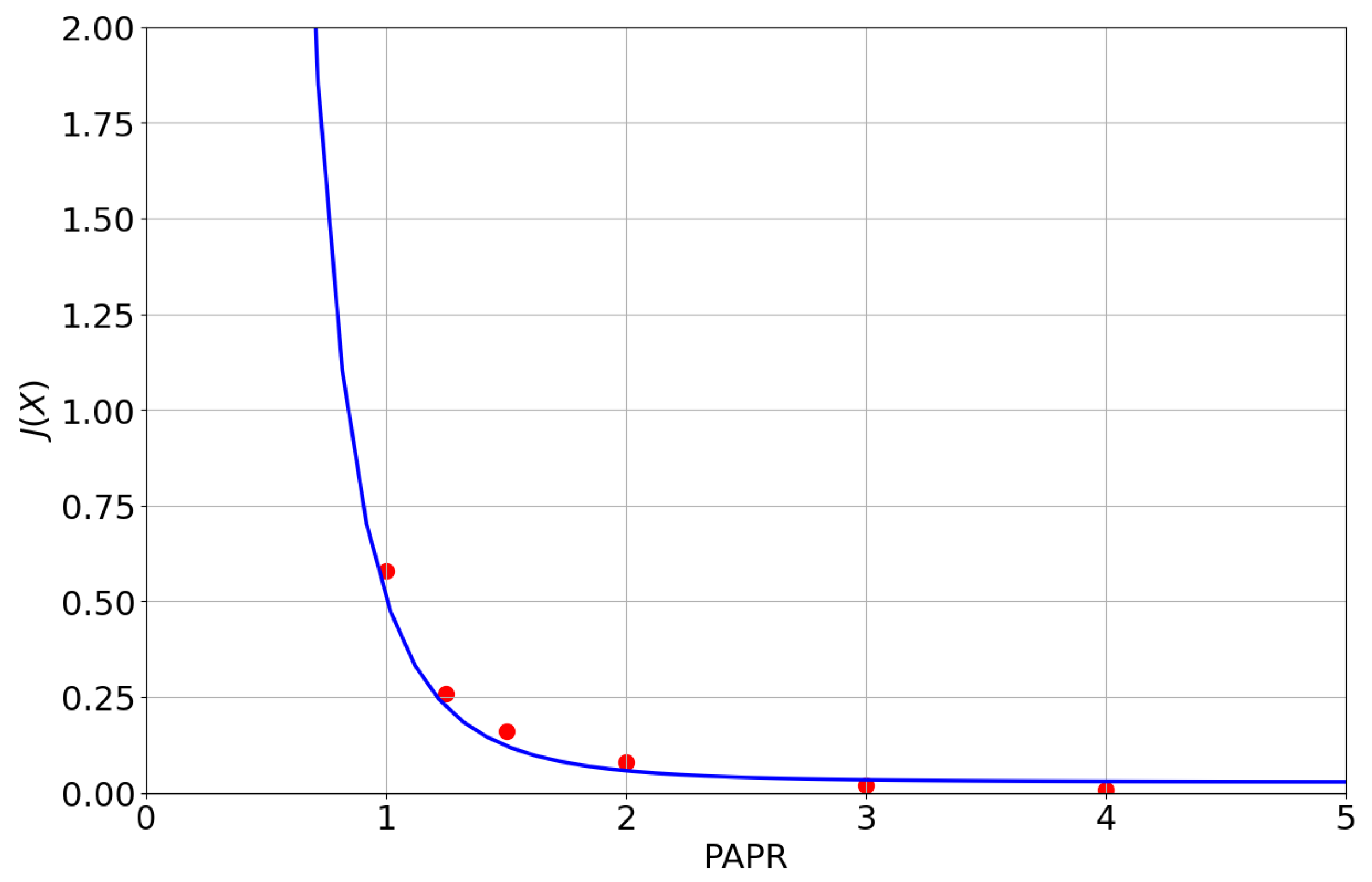
• The randomness of the envelope may cause the transmitter to experience a decline in efficiency: higher peaks when compared to the average power of the envelope lead to lower transmitter performance. Thus, PAPR is used to optimize these waveforms.

  $$\mathrm{PAPR}={\displaystyle \frac{{max}_n{\left|x\left[n\right]\right|}^2}{\frac{1}{N}{\sum }_{n=1}^N{\left|x\left[n\right]\right|}^2}},$$

  (3)

  where $x\left[n\right]$ is the discrete version of the complex envelope, which is usually defined as a complex exponential $x\left(t\right)=e^{j\varphi \left(t\right)}$, B is the bandwidth, and N is the number of samples, which is the product of the sampling frequency and the integration time: $N=f_s\tau$. Figure 1 illustrates how a high PAPR affects SNR [9]; ideally, we want PAPR close to 1.

2.2. NRT Waveform Design

Waveform design in NRT has received some recent attention due to the need to enhance its correlation properties, coupled with the increase in its computational capacity. In [11], noise signals were generated by introducing noise to a linear frequency modulation (LFM) chirp; yet, the traditional way to generate NRT waveforms is by introducing Gaussian independent, identically distributed (iid) samples into the phase of a unimodular sequence or into the in-phase (I) and quadrature (Q) components. This sequence is then optimized, usually by filtering in the Fourier domain with a spectral shape equal to the square root of a window function, $H\left(n\right)=\sqrt{w\left(n\right)}$. Several algorithms have been proposed to minimize PAPR while maintaining a low-range sidelobe level, namely BLASA (band-limited algorithm for sidelobes attenuation [12]) and COSPAR (combined spectral shaping and peak-to-average power reduction [13]).

BLASA aims to attenuate the range sidelobes while keeping the spectral shape within given bounds, defining PAPR as a constraint for marine pulsed radar systems. Based on the CAN (cyclic algorithm new) family of algorithms [14], BLASA approach minimizes a value that expresses the difference between a representation of the ACF and the desired one. The authors also present a BLASA MIMO version.

COSPAR approaches the problem in a different way: the authors propose generating a Taylor window spectral shape, adding a random phase component in the Fourier domain, and finally implementing a PAPR reduction algorithm, based on the Gerchberg–Saxton algorithm [15], which aims to maintain the ACF shape.

Finally, FMeth [9] was proposed to reduce the range sidelobes in a specific lag interval close to the mainlobe, using a concept based on inverse filtering. For more in-depth information, [16] provides an extensive understanding in signal design for NRT.

2.3. Noise Radar Recognition

We have already partly addressed how NRT fits into the LPI category. However, there are several other techniques that may be exploited by a LPI system, such as frequency agility or low power transmissions. Modern highly sensitive ESM systems tackle this challenge by employing advanced signal analysis and time–frequency techniques. The latter is a robust approach used to analyze signals in both the time and frequency domains simultaneously, providing insight into how signal properties evolve over time. These methods are representations of the energy distribution along time and frequency. Examples include the Wigner–Ville distribution (WVD) [17], the Choi–Williams distribution (CWD) [18], the short-time Fourier transform (STFT) [19], and continuous wavelet transform (CWT) [20]. However, the time–frequency power distribution of a NRT signal is ideally similar to a noise distribution, so it is hard to distinguish between them.

Noise radar classification has also been researched to some extent. Spectral kurtosis was used to classify noise radar waveforms [21]; this is a statistical measure used to describe the shape of the distribution of a signal, which quantifies how the spectral content of a signal deviates from a Gaussian distribution. Higher values of spectral kurtosis indicate sharper peaks in the spectrum, while lower values suggest a flatter spectral distribution.

2.4. Waveform Entropy

It was already discussed above how time–frequency analysis is implemented to detect LPI radar systems. However, relative entropy, or Kullback–Leibler divergence, is becoming a popular metric for detecting LPI signals, since it has the ability to provide a direct measurement of how much one probability distribution deviates from another. This is not only useful for implementation in ESM systems [22] but also for adaptive techniques [23] and, as proposed in this paper, to design noise radar waveforms.

The Kullback–Leibler divergence (KLD) is defined as

$$D_{\mathrm{KL}}(f_1\left(x\right)\Vert f_2\left(x\right))={\int }_{-\infty }^{+\infty }{f}_1\left(x\right)log{\displaystyle \frac{f_1\left(x\right)}{f_2\left(x\right)}}dx,$$

(4)

where $f_1\left(x\right)$ and $f_2\left(x\right)$ are the probability density functions (PDF) to be compared. This is achieved in practice by taking the eigenvalue vectors of the standardized mean vector and covariance matrix of both the waveform to be evaluated and Gaussian noise.

Negentropy is a related concept based on differential entropy, which can be used to design waveforms. The main difference is that negentropy is a measure of how much a distribution deviates from a Gaussian distribution with the same variance. Since the power of the waveform is known, negentropy is a useful concept, and straightforward to estimate by evaluating the third and fourth moments of the sequence.

Assume that the designed waveform $x\left(n\right)$ is a realization of random variable X with PDF $f\left(x\right)$. Then, its differential entropy is

$$H\left(X\right)=-\mathbb{E}[logf\left(x\right)]=-{\int }_{x}f\left(x\right)logf\left(x\right)dx.$$

(5)

Negentropy is obtained by subtracting the estimated differential entropy from the entropy of a Gaussian PDF,

$$J\left(X\right)=H_G\left(X\right)-H\left(X\right),$$

(6)

where $H_G\left(X\right)$ is the differential entropy of a Gaussian with variance ${\sigma }^2$, well known to be $H_G\left(X\right)={\displaystyle \frac{1}{2}}\ln \left(2\pi e{\sigma }^2\right)$. If X is non-Gaussian, negentropy can be approximated using higher-order statistics; a common approximation is

$$J\left(X\right)\approx {\displaystyle \frac{1}{12}}{\left(\mathbb{E}\left[X^3\right]\right)}^2+{\displaystyle \frac{1}{48}}{\kappa }^2,$$

(7)

where $\mathbb{E}\left[X^3\right]$ is the third moment of X and $\kappa$ is the kurtosis of X [24,25].

Since the kurtosis is the fourth standardized moment $\kappa =\mathbb{E}\left[X^4\right]/{\sigma }^2$, for a signal represented by a zero-mean random variable X (where the average power $P_{\mathrm{avg}}$ coincides with the variance ${\sigma }^2$), the variance can be expressed as a function of PAPR:

$$\mathrm{Var}\left(X\right)={\displaystyle \frac{{max\left|X\right|}^2}{\mathrm{PAPR}}}.$$

(8)

Moreover, kurtosis can be expressed as a function of PAPR, and the approximation of negentropy in Equation (7) becomes

$$J\left(X\right)\approx {\displaystyle \frac{1}{12}}{\left(\mathbb{E}\left[X^3\right]\right)}^2+{\displaystyle \frac{1}{48}}{\left(\left(\mathbb{E}\left[X^4\right]\right)·{\displaystyle \frac{P_{\mathrm{peak}}^2}{{\mathrm{PAPR}}^2}}\right)}^2,$$

(9)

where $P_{\mathrm{peak}}$ is the maximum value of the waveform sequence. Notice that PAPR is not injective: each possible X does not lead to a unique PAPR, i.e., there are different signals that are unimodular (PAPR = 1). Therefore, negentropy cannot be written as a function of PAPR alone for the full set of solutions, being instead jointly influenced by both PAPR and the higher-order moments of the signal distribution.

From Equation (9), illustrated in Figure 2, we can conclude that minimizing the distance of both high-order moments of the generated waveform to the Gaussian ones minimizes negentropy. Furthermore, as illustrated by the red points in Figure 2, we add the simulation results obtained in [16] for an estimation of negentropy using the histogram approximation of the PDF of a single noise waveform with a uniform spectrum, $50\mathrm{MHz}$ bandwidth, and $0.5$ variance. Consequently, we validate our theoretical expression and conclude that Equation (9) accurately fits the waveforms in [16] for fixed values of high-order moments of X: $\mathbb{E}\left[X^3\right]\cong 0.55$, $\mathbb{E}\left[X^4\right]\cong 4.80$, and $P_{\mathrm{peak}}=1$. Note that PAPR cannot define a function of X alone; for each case, it is necessary to estimate the distinct parameters represented in Equation (9). Furthermore, note that the approximation in Equation (7) suffers from non-robustness due to the need to estimate kurtosis. Therefore, the approximation in Equation (9) is more accurate for kurtosis values close to 3. Moreover, it is important to keep in mind that generating noise signals by designing a random phase and implementing a complex exponential is different that generating iid I and Q components. The kurtosis of the complex exponential is close to 0, since it maps a real Gaussian distributed sequence to a non-Gaussian distribution in the complex plane. Moreover, it is important to keep in mind that generating noise signals by designing a random phase and applying a complex exponential is different from generating iid I and Q components. The resulting complex exponential signal has a non-Gaussian distribution with a constant amplitude and a uniformly distributed phase, unlike a Gaussian distribution in the complex plane produced by iid I and Q components.

For iid Gaussian I and Q components, the amplitude distribution of the resulting complex signal has a higher kurtosis, often around 3. In contrast, the constant–amplitude nature of the complex exponential can lead to a lower effective kurtosis for any real-valued projection of the signal. In the following section, we chose to implement the former option since the complexity of the proposed algorithm decreases polynomially with the number of samples.

3. Multi-Objective Optimization Problem Formulation

We formulate waveform design as a multi-objective optimization problem (MOP), as described in this section. The MOP allows for a structured approach to balance the competing goals, ensuring a comprehensive evaluation of potential solutions. In the context of this study, we consider the transmitted signal defined as

$$x\left(t\right)=a\left(t\right)e^{j\varphi },\varphi \in [-\pi ,\pi ],$$

(10)

with $a\left(t\right)$ denoting the amplitude, where a windowing function can be implemented in the time domain. We use this approach instead of generating Gaussian iid I and Q components since its quicker to optimize a vector of size N instead of $2N$. Thus, in discrete time, we work with vectors $\mathit{a}=\left[a\right(0),a(1),...,a(N-1\left)\right]$ and $\mathit{\varphi }=\left[\varphi \right(0),\varphi (1),...,\varphi (N-1\left)\right]$:

$${\mathit{x}}_a=[x_a\left(0\right),...,x_a(N-1)]=\mathit{a}\odot e^{j\mathit{\varphi }},$$

(11)

where ⊙ is the Hadamard element-wise product. ${\mathit{x}}_a$ is the initial $\mathit{x}$ before the Fourier transforms.

The signal $\mathit{x}$ is then obtained by shaping in Fourier domain with a desired window function $\mathit{w}$ limited in the baseband bandwidth between ${\displaystyle \frac{-B}{2}}$ and ${\displaystyle \frac{B}{2}}$,

$$\mathit{x}={\mathcal{F}}^{-1}\{\mathcal{F}\left({\mathit{x}}^{\prime }\right)\odot \mathit{w}\},$$

(12)

with $\mathcal{F}$ and ${\mathcal{F}}^{-1}$ standing for the discrete Fourier transform (DFT) and inverse DFT (IDFT), respectively.

In the MOP, we use as metrics PAPR (Equation (3)) and in order to minimize the sidelobe level, the integrated sidelobe level (ISL) expresses the power of the ACF sidelobes,

$$\mathrm{ISL}={\displaystyle \frac{1}{|r_0{|}^2}}\sum _{n\ne 0}{\left|r_n\right|}^2,$$

(13)

where r is the autocorrelation function (see Equation (1)), which may be computed efficiently in the Fourier domain,

$$\mathit{r}={\mathcal{F}}^{-1}\{\mathcal{F}\left(\mathit{x}\right)\odot {\mathcal{F}}^{*}\left(\mathit{x}\right)\},$$

(14)

where ${(·)}^{*}$ denotes complex conjugation. Hence, the MOP aiming at minimizing ISL and PAPR can be written as:

$$\left\{\begin{array}{cc}{\mathrm{minimize}}_{\mathit{\varphi }}\hfill & \mathrm{ISL}\hfill \\ {\mathrm{minimize}}_{\mathit{\varphi }}\hfill & \mathrm{PAPR}\hfill \\ \mathrm{subject}\mathrm{to}\hfill & -\pi \le {\varphi }_n\le \pi ,\hfill \end{array}\right.$$

(15)

where the notation denotes solving the MOP over the vector variable $\mathit{\varphi }$.

Shaping a non-deterministic sequence leaves deterministic information that is transmitted along with the waveform. Therefore, ambiguity function (AF) analysis allows us to understand better this behavior. It provides information about the potential range and Doppler ambiguities in a radar signal and is crucial for radar system design and analysis, helping to understand the trade-offs between range and Doppler resolution:

$$A(m,f_d)=\sum _{n=0}^{N-1}x\left[n\right]x^{*}[n-m]e^{-j2\pi f_{d}n}.$$

(16)

To better understand how the AF is impacted by implementing deterministic sequences, Figure 3 shows the plot for a frequency modulated signal, while Figure 4 showcases the AF of Gaussian-distributed noise.

One of the main purposes of using NRT is to keep it as undetectable as possible. Apart from analyzing the AF of a sequence, negentropy has been introduced to keep an NRT sequence as random as possible, by studying how it impacts PAPR [16]. Besides proposing the use of MOE to design NRT waveforms, we introduce the use of negentropy as a constraint in the MOP. Finally, the the MOP that will be tackled is

$$\left\{\begin{array}{cc}{\mathrm{minimize}}_{\mathit{\varphi }}\hfill & \mathrm{ISL}\hfill \\ {\mathrm{minimize}}_{\mathit{\varphi }}\hfill & \mathrm{PAPR}\hfill \\ \mathrm{subject}\mathrm{to}\hfill & -\pi \le {\varphi }_n\le \pi \hfill \\ \mathrm{subject}\mathrm{to}\hfill & J\left(X\right)<\alpha ,\hfill \end{array}\right.$$

(17)

where $\alpha$ is a preset value defined beforehand. In this work, we will study it in the interval $(0,1.8]$: values between 0 and 1.8, excluding 0. This interval is chosen because when optimizing without constraints, the negentropy values are always less than $1.8$. Therefore, it would be pointless to use a constraint value larger than the latter.

4. Algorithm Description

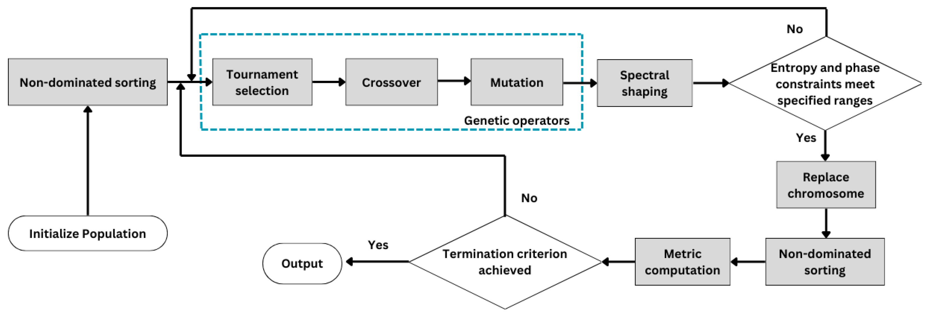
Before describing the proposed MOE algorithm, we introduce the family of techniques it belongs to and how it applies to our problem. Evolutionary algorithms (EAs) are heuristic search techniques inspired by Darwinian evolution, which have the robustness and flexibility to find global solutions to challenging optimization problems. Although there are significant differences in how the evolutionary mechanisms are applied, all of the EA variants share a common fundamental idea: the existence of a population of individuals exposed to environmental pressure resulting in selection that is usually achieved by having the populations average fitness increase as a result of survival of the fittest.

Accordingly, when an EA is used to solve a problem requiring the optimization of two or more potentially conflicting objectives, it is called a MOE algorithm. Unlike single-objective optimization algorithms, MOEAs do not converge to one optimal solution. Instead, a MOP has a set of optimal solutions—called a Pareto set—which are also called non-inferior, admissible, or efficient solutions. The non-dominated vectors, when plotted in objective space, are known as the Pareto front (PF).

Designing radar waveforms using MOE algorithms is not a new idea. In fact, in [26,27], the authors studied the application of several MOE algorithms for phase-coding a waveform maximizing the probability of detection and minimizing the Cramer–Rao lower bound (CRLB) on the variance of the frequency estimate to improve Doppler accuracy.

The next section will describe the proposed algorithm from the aforementioned family and how we applied it to our problem, which is designing a sequence by solving the MOP already discussed in Section 2.

SS-NSGA Description

The proposed algorithm, called spectral shaping non-dominated sorting genetic algorithm (SS-NSGA) is rooted in the NSGA-II algorithm. The latter is a popular EA proposed in [8] that excels for its speed, with computation complexity $O\left(M{A}^2\right)$ where M is the number of objectives and A is the population size.

The SS-NSGA maintains a population of candidate solutions represented as individuals. It implements a non-dominated sorting technique to rank individuals based on their Pareto dominance relationship, where one solution is better if it has at least one objective better than another solution, and all the others are not worse. To maintain diversity within each Pareto front, it calculates the crowding distance for each solution, which is a measure of the average distance between the solution itself and its neighbors in the objective space. Then, it implements elitist selection, crossover, and mutation operations to enhance diversity and convergence of solutions over each generation. Thereafter, the resulting waveform sequences are shaped in the Fourier domain with a Taylor window, while constraining the result vector to the phase of the complex exponential waveform and negentropy values represented in Equation (17). The algorithm continues until a termination criterion is met, such as achieving a desired objective value or reaching a specified number of generations. Figure 5 shows a summarized flowchart of SS-NSGA.

Besides having success in many real world problems, NSGA-II is chosen out of other algorithms, such as strength Pareto evolutionary algorithm 2 (SPEA2) and multi-objective evolutionary algorithm, based on decomposition (MOEA/D), because of its computational efficiency, since we are dealing with a very demanding problem, and its ability do search for diverse solutions by evaluating its crowding distance.

5. Experiments

5.1. Experiment Design

The experiments are divided into two main phases:

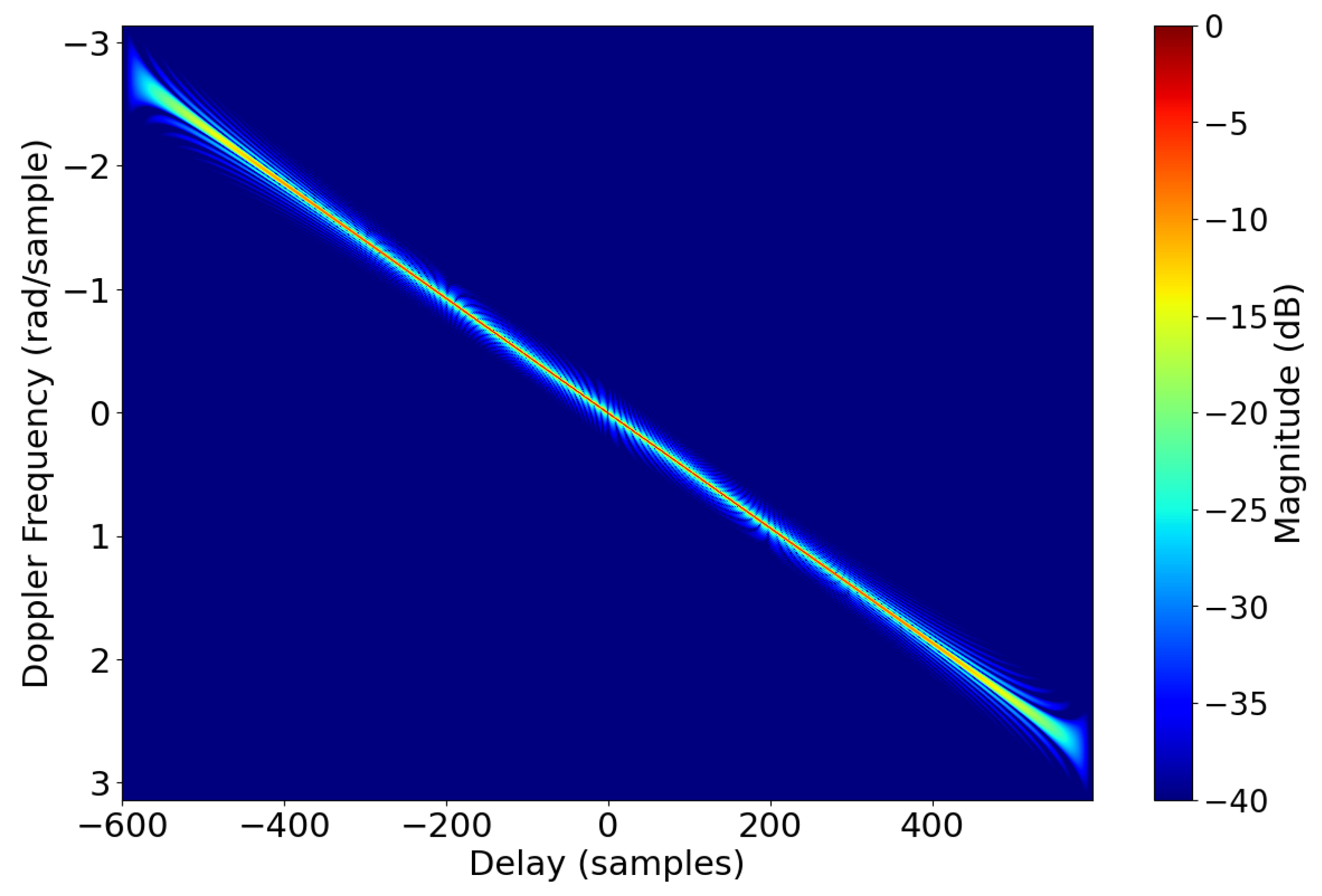
• First, the problem is solved subject to Equation (15), reaching a set of Pareto optimal solutions and plotting its AF;
• Then, the problem is solved as described in Equation (17). Negentropy $J\left(X\right)$ is set to a set of values $\alpha \in [0,1.8]$ and a new metric $\beta =\mathrm{ISL}+10\mathrm{PAPR}$ is presented as a function of the chosen negentropy. This metric is chosen particularly by scaling PAPR up, since the values of the ISL typically register one decimal place higher.

In order to create an unbiased study, all the algorithm parameters are the same for the two cases. The initial population of $\mathit{\varphi }$s is generated randomly with a Gaussian distribution. Then, it is evaluated by solving Equation (12) with $\mathit{a}$ as a unit vector and $\mathit{w}$ as a Taylor window [28] with coefficients limited from $-B/2$ to $B/2$, allowing the solution to be constrained in a certain bandwidth and with the desired shape. The termination criterion is the number of generations, which is the same for all trials. The genetic operators used are: binary tournament selection based on the crowded-comparison operator [29], simulated binary crossover [30], and polynomial mutation [31].

We assume a bandwidth of B = 100 MHz, a sampling frequency at the analog-to-digital converter (ADC) of $f_s$ = 200 MHz and a time duration of T = 6 μs. Therefore, the waveform has $N=f_s·T$ = 1200 samples.

MOEAs and SS-NSGA are stochastic algorithms. Therefore, for vast amounts of data such as radar waveforms, there is a need for a large number of evaluations. In our experiment, the algorithm converges following a logarithmic trend due to its inherent structure and the computational steps involved in each evaluation. We could observe that for the 1200 samples, we needed to run it 10,000 times, which translates to around one hour of runtime on a common laptop. It is essential to understand that this hour of processing time generate us around 1000 distinct signals which is directly related to the population size. Furthermore, real-time generations is not desired for our case, since we may store a set of thousands of waveforms before transmission.

When up-sampling the waveform to the Nyquist rate, interpolation anomalies may be introduced which increase PAPR, leading to inefficiencies in power usage and potential distortions. These unintended distortions occur since up-sampling involves inserting additional samples between the original ones, which can create new peaks if not managed properly, increasing PAPR by 2–3 dB [13]. Incorporating techniques such as low-pass filtering during up-sampling or designing waveforms directly at the higher sampling rate can be implemented to mitigate these issues. In this work, we opted to work with a waveform directly at the higher sampling rate (Nyquist rate). However, the bandwidth of the optimized signal could be higher, leading to potential issues such as the DAC not being able to deal with such high sampling frequencies. Consequently, as a way to mitigate these potential issues, we added a weight of 10 to the PAPR objective, generating waveforms with a lower PAPR of approximately 1.3, giving more flexibility to the up-sampling potential effects.

5.2. Results

When tackling the problem in Equation (15), the algorithm converges to the Pareto front displayed in Figure 6. We can generate thousands of solutions, i.e., different waveforms, with a PAPR between $1.1$ and $1.6$, while maintaining it constrained to a certain bandwidth and minimizing the range sidelobes, as can be seen in Figure 7. We compare our results to the well-known CAN algorithm [14] to generate unimodular noise waveforms, and conclude that the average of all the signals generated has a similar sidelobe level with a PAPR of $1.15$. Furthermore, we introduce negentropy to design noise radar waveforms and leave versatility in the algorithm to implement other constraints or objectives. Additionally, from Figure 8, we can conclude that the average of all the final population performs slightly worse than the CAN algorithm. However, the best solution out of the population slightly outperforms CAN.

When comparing to the well-known algorithms for noise radar waveform design previously discussed, the following conclusions can be drawn:

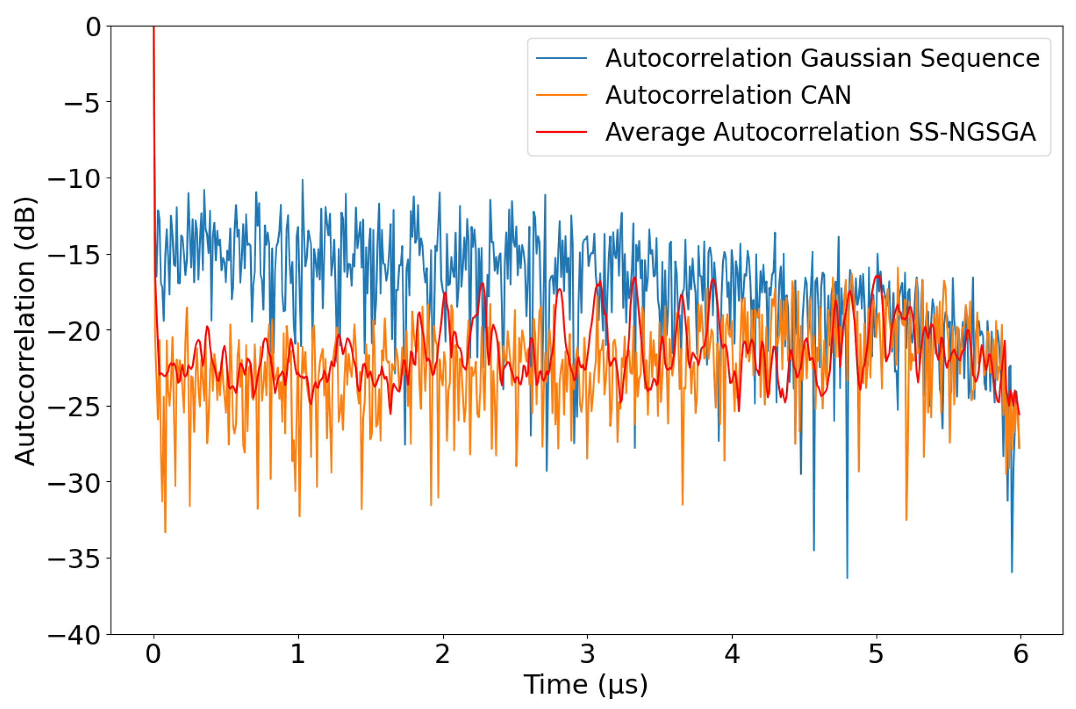
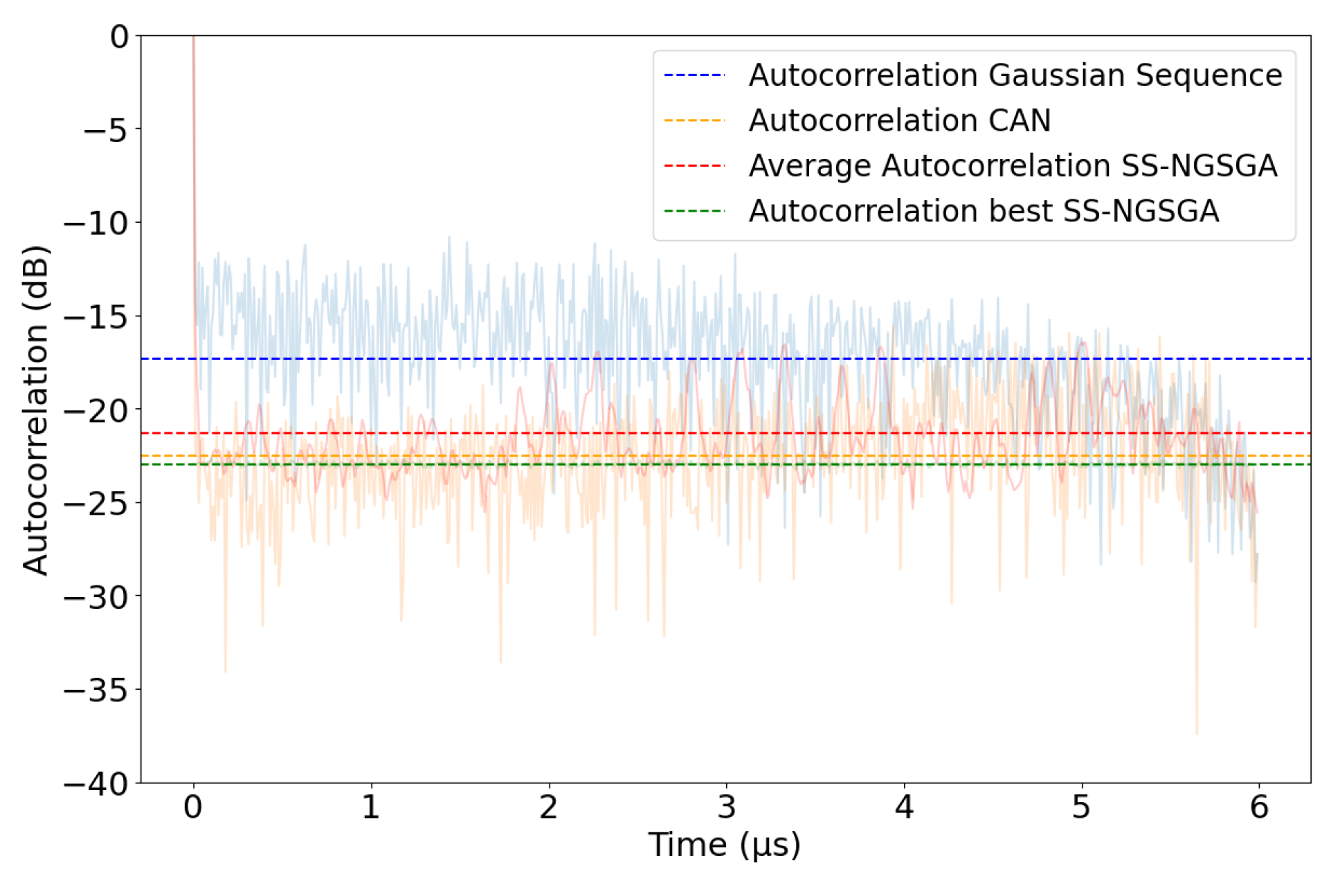
• BLASA [12] exhibits performance comparable to CAN regarding sidelobe level of the ACF. Consequently, our best solution may outperform the latter algorithm by approximately 1 dB (see Figure 8). However, the LPI properties of BLASA, and by this we mean the time–frequency representation, are closer to Gaussian noise than our algorithm without any constraints.
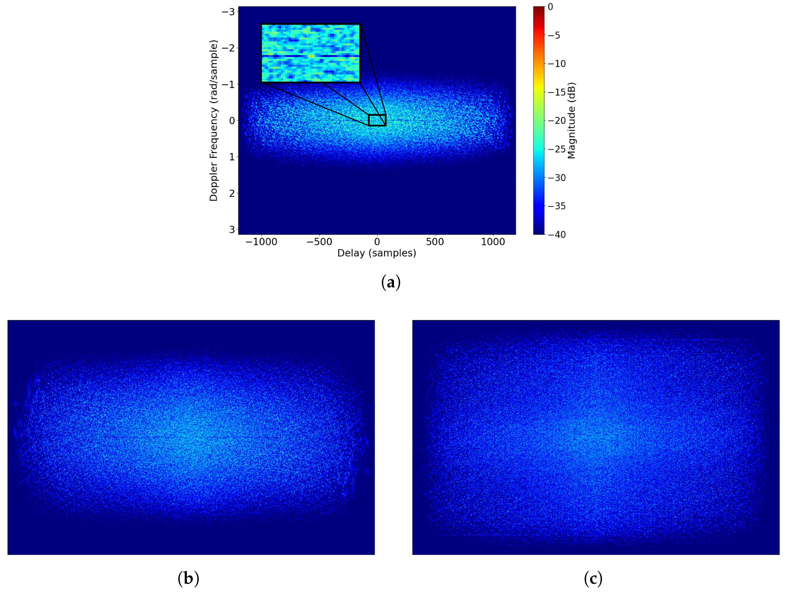
• COSPAR [13] performs better than our algorithm for the same PAPR, where for a fixed time–bandwidth product, the values depend on the chosen sidelobe level of the Taylor window. However, besides COSPAR achieving a great value of spectral kurtosis, which is a way to detect noise radar synthesized waveforms, our algorithm allows for time–frequency representation that is closer to a Gaussian distribution.

To demonstrate this claim, we make a comparison of the time–frequency representations of COSPAR, CAN and our method to the representation of a Gaussian sequence. For each method, the ambiguity function plot of the optimized sequence is computed, converted to grayscale, resized, and normalized. Then, the Kullback–Leibler divergence is calculated as in Equation (4), where the PDF represented by $f_1\left(x\right)$ and $f_2\left(x\right)$, are now matrices expressing the normalized grayscale pixels of the image of the evaluated method and the Gaussian sequence, respectively. Observe that zero KLD indicates that the signal is identical to the Gaussian reference time–frequency image, whereas greater values suggest a more distant representation from the reference one.

Figure 9 illustrates COSPAR, CAN, our method without constraint, and with a negentropy constraint of 0.2 and 0.9. Although COSPAR achieves spectral kurtosis values close to 0, it performs similarly to our method regarding KLD. CAN performs better than both methods, but when we constrain the optimization problem with negentropy values, we can lower KLD significantly, with a cost of ISL (see Figure 9).

In summary, whilst both BLASA and COSPAR yield commendable results suitable for varied applications, this paper introduces an algorithm that occupies an intermediate position and can be tailored to specific requirements. Although the proposed algorithm may outperform BLASA or COSPAR in certain metrics, it does not excel in all metrics simultaneously. Most importantly, this work introduces the concept of negentropy to design noise sequences which can be utilized by radar systems, and an algorithm that can be customized to a specific environment: giving more emphasis on the sidelobe levels of the ACF, or on the LPI features.

On the second experiment already described, the algorithm ran for different values of the negentropy upper bound (see Equation (17)). The results are plotted in relation to the metric $\beta$ and are displayed in Figure 10. The obtained results are similar to the ones simulated in [16] for a varying PAPR. We can achieve $J\left(X\right)$ close to 0 with PAPR = 4. Yet, the sidelobe levels achieved are too high, making the waveform unusable, with our metric achieving very high values.

To better understand how the sidelobes and AF are impacted by constraining the waveform to a certain $J\left(X\right)$, Figure 11a displays the AF for an optimized waveform without any constraint and the AF for $J\left(X\right)=0.9$ and $J\left(X\right)=0.2$ in Figure 11b,c, respectively. We see that the more we constrain the optimization problem, the more the shape of the AF gets closer to that of a Gaussian random sequence. Hence, besides achieving good performance for solving the stand-alone MOP, we derived a solution for shaping the AF, that can be applied to various situations and be an object for studying NRT radar recognition and performance of ESM systems.

5.3. Time–Frequency Analysis

As discussed in the Introduction, modern ESM systems may employ time–frequency analysis techniques to classify LPI radars. Some authors already discussed this topic for NRT waveforms, as in [13]. Nonetheless, we choose to analyze our generated waveform with respect to its STFT and CWT, since both provide different information on how frequency varies with time, complementing each other. STFT maintains the same resolution for time and frequency, while CWT enables to observe transient information associated with amplitude and phase shifts, giving better frequency resolution for long scales and time resolution for short scales. This is achieved by introducing a scaling parameter a and having a wavelet ${\psi }^{*}$ with finite-time support:

$$W(a,\tau )={\int }_{-\infty }^{\infty }x\left(t\right)·{\displaystyle \frac{1}{\sqrt{a}}}{\psi }^{*}\left({\displaystyle \frac{t-\tau }{a}}\right)dt.$$

(18)

Figure 12a displays the STFT of the designed waveform. We have chosen to display the less noise-like waveform from the generated dataset of signals and we still see that it is similar to noise by being spread across the time–frequency plane. We also demonstrate that we can shape the ambiguity function (Figure 11) and, consequently, the STFT, by constraining the optimization problem, which can enhance the LPI properties at the cost of higher ISL and PAPR.

In the CWT analysis, we use the Morlet wavelet [32], which is a widely used continuous wavelets in time–frequency analysis that provides a good compromise between time and frequency resolution. The CWT of Gaussian noise is displayed in Figure 13c. We observe that our waveform, similarly to the STFT analysis, is spread across the time–frequency plane. However, it has a cluster of energy over the high-frequency components. This may be an object of study in future work, whether we can implement time–frequency analysis to detect these waveforms or not. Also, by constraining the MOP, we can change the CWT of the signal pattern close to that of Figure 13c.

6. Conclusions and Future Work

We have discussed how noise radar differs from conventional radar, its advantages and waveform design challenges. Subsequently, we explored the ongoing efforts to tackle these issues and proposed a new method for solving the range sidelobe level while maintaining a desired PAPR.

While multi-objective evolutionary algorithms have previously been used to solve radar waveform design challenges, such as designing optimal phase codes, we propose an implementation of these techniques to address larger sequences in noise radar waveform design, accompanied by an additional study of how negentropy constraints affect the results. We introduced the use of evolutionary algorithms for noise radar technology waveform design, but most importantly, we demonstrate that negentropy can be used to design noise radar waveforms. Furthermore, we derive an expression to estimate negentropy based on waveforms’ high-order moments and PAPR, validating it with simulation results from other authors.

The signals that result from the optimization algorithm are not entirely non-deterministic. Instead, they are tailored and consequently lose some of their characteristics, which is why low-probability-of-intercept analysis and experiments are important. Hence, we conducted a time–frequency analysis in Section 5.3 on the optimized signal and compared it to Gaussian noise and the well-known linear chirp. Most importantly, we incorporated negentropy as a randomness constraint to tailor the ambiguity function and enhance the low-probability-of-intercept characteristics of the waveform, although with a trade-off in integrated sidelobe level and peak-to-average power ratio. In doing so, we established a method to tailor waveforms for specific low-probability-of-intercept characteristics, which is an important tool and opens avenues for future research, from noise radar technology classification to adaptive techniques. Moreover, when the algorithm is executed for a sufficient duration, the optimal solution within the population not only marginally surpasses the performance of well-known cyclic algorithms but also ensures that the average performance of the population remains comparable to these algorithms.

Looking forward, and being aware that this is not a real-time implementation, at least with a computer, we want to address the application of parallel processing techniques or implementation on a field-programmable gate array allowing for real-time generation and implementation of adaptive techniques. We also want to address noise radar waveform design for multiple-input multiple-output radar, and to implement this waveform in a real environment testing it against real electronic support measures systems.

References

1. Ankel, M.; Jonsson, R.; Bryllert, T.; Ulander, L.M.H.; Delsing, P. Bistatic noise radar: Demonstration of correlation noise suppression. IET Radar Sonar Navig. 2023, 17, 351–361. [Google Scholar] [CrossRef]
2. Lai, C.P.; Narayanan, R.M. Ultrawideband Random Noise Radar Design for Through-Wall Surveillance. IEEE Trans. Aerosp. Electron. Syst. 2010, 46, 1716–1730. [Google Scholar] [CrossRef]
3. Meller, M.; Tujaka, S. Processing of Noise Radar Waveforms using Block Least Mean Squares Algorithm. IEEE Trans. Aerosp. Electron. Syst. 2012, 48, 749–761. [Google Scholar] [CrossRef]
4. Sénica, A.L.; Marques, P.A.C.; Figueiredo, M.A.T. Artificial Intelligence Applications in Noise Radar Technology. IET Radar Sonar Navig. 2024, 18, 986–1001. [Google Scholar] [CrossRef]
5. Thayaparan, T.; Spaans, A. Noise Radar Technology Basics; Technical Memorandum; Defence R&D Canada: Ottawa, ON, Canada, 2006; Available online: https://apps.dtic.mil/sti/tr/pdf/ADA462896.pdf (accessed on 31 January 2025).
6. Savci, K.; Stove, A.G.; De Palo, F.; Erdogan, A.Y.; Galati, G.; Lukin, K.A.; Lukin, S.; Marques, P.; Pavan, G.; Wasserzier, C. Noise Radar—Overview and Recent Developments. IEEE Aerosp. Electron. Syst. Mag. 2020, 35, 8–20. [Google Scholar] [CrossRef]
7. Galati, G.; Pavan, G. Noise Radar Technology as an Interference Prevention Method. J. Electr. Comput. Eng. 2013, 2013, 146986. [Google Scholar] [CrossRef]
8. Deb, K.; Pratap, A.; Agarwal, S.; Meyarivan, T. A fast and elitist multiobjective genetic algorithm: NSGA-II. IEEE Trans. Evol. Comput. 2002, 6, 182–197. [Google Scholar]
9. Palo, F.D.; Galati, G.; Pavan, G.; Wasserzier, C.; Savci, K. Introduction to noise radar and its waveforms. Sensors 2020, 20, 5187. [Google Scholar] [CrossRef]
10. Turin, G. An introduction to matched filters. IRE Trans. Inf. Theory 1960, 6, 311–329. [Google Scholar]
11. Govoni, M.A.; Li, H.; Kosinski, J.A. Range-Doppler resolution of the linear-FM noise radar waveform. IEEE Trans. Aerosp. Electron. Syst. 2013, 49, 658–664. [Google Scholar] [CrossRef]
12. De Palo, F.; Galati, G. Range sidelobes attenuation of pseudorandom waveforms for civil radars. In Proceedings of the 2017 European Radar Conference (EURAD), Nuremberg, Germany, 11–13 October 2017; pp. 114–117. [Google Scholar]
13. Savci, K.; Galati, G.; Pavan, G. Low-PAPR waveforms with shaped spectrum for enhanced low probability of intercept noise radars. Remote Sens. 2021, 13, 2372. [Google Scholar] [CrossRef]
14. He, H.; Li, J.; Stoica, P. Waveform Design for Active Sensing Systems: A Computational Approach; Cambridge University Press: Cambridge, UK, 2012. [Google Scholar]
15. Gerhberg, R.; Saxton, W. A practical algorithm for the determination of phase from image and diffraction plane picture. Optik 1972, 35, 237–246. [Google Scholar]
16. Galati, G.; Pavan, G.; Wasserzier, C. Signal design and processing for noise radar. EURASIP J. Adv. Signal Process. 2022, 2022, 52. [Google Scholar]
17. Ville, J. Theorie et applications de la notion de signal analytique. Cables Transm. 1948, 1, 61–74. [Google Scholar]
18. Choi, H.I.; Williams, W.J. Improved time-frequency representation of multicomponent signals using exponential kernels. IEEE Trans. Acoust. Speech Signal Process. 1989, 37, 862–871. [Google Scholar] [CrossRef]
19. Cohen, L. Time-Frequency Analysis; Prentice Hall PTR: Englewood Cliffs, NJ, USA, 1995; Volume 778. [Google Scholar]
20. Aguiar-Conraria, L.; Soares, M.J. The continuous wavelet transform: Moving beyond uni-and bivariate analysis. J. Econ. Surv. 2014, 28, 344–375. [Google Scholar] [CrossRef]
21. Çotuk, N.; Kayran, A.H.; Aytun, A.; Savci, K. Detection of Marine Noise Radars with Spectral Kurtosis Method. IEEE Aerosp. Electron. Syst. Mag. 2020, 35, 22–31. [Google Scholar]
22. Zhao, M.; Xu, S.; Sun, B. Evaluation of Waveform RF Stealth Performance Based on Relative Entropy. In Proceedings of the 8th International Conference on Communication and Information Processing, ICCIP ’22, Beijing, China, 3–5 November 2022; pp. 156–162. [Google Scholar] [CrossRef]
23. Ziemann, M.R.; Metzler, C.A. Adaptive LPD Radar Waveform Design with Generative Adversarial Neural Networks. In Proceedings of the 2023 57th Asilomar Conference on Signals, Systems, and Computers, Pacific Grove, CA, USA, 29 October–1 November 2023; pp. 1039–1043. [Google Scholar]
24. Jones, M.C.; Sibson, R. What is projection pursuit? J. R. Stat. Soc. Ser. A 1987, 150, 1–18. [Google Scholar] [CrossRef]
25. Bühlmann, V. Negentropy. In Posthuman Glossary; Bloomsbury Academic: London, UK, 2018; pp. 273–277. [Google Scholar]
26. Stringer, J.; Lamont, G.; Akers, G. Radar phase-coded waveform design using MOEAs. In Proceedings of the 2012 IEEE Congress on Evolutionary Computation, Brisbane, Australia, 10–15 June 2012; pp. 1–8. [Google Scholar]
27. Chopra, A. Association Control Based Load Balancing in Wireless Cellular Networks Using Preamble Sequences. Ph.D. Thesis, Open Access Te Herenga Waka-Victoria University of Wellington, Wellington, New Zealand, 2012. [Google Scholar]
28. Taylor, T.T. Design of line-source antennas for narrow beamwidth and low side lobes. Trans. Ire Prof. Group Antennas Propag. 1955, 3, 16–28. [Google Scholar] [CrossRef]
29. Goldberg, D.E.; Deb, K. A comparative analysis of selection schemes used in genetic algorithms. In Foundations of Genetic Algorithms; Elsevier: Amsterdam, The Netherlands, 1991; Volume 1, pp. 69–93. [Google Scholar]
30. Deb, K.; Sindhya, K.; Okabe, T. Self-adaptive simulated binary crossover for real-parameter optimization. In Proceedings of the 9th Annual Conference on Genetic and Evolutionary Computation, GECCO ’07, London, UK, 7–11 July 2007; pp. 1187–1194. [Google Scholar] [CrossRef]
31. Deb, K.; Agrawal, R.B. Simulated binary crossover for continuous search space. Complex Syst. 1995, 9, 115–148. [Google Scholar]
32. Lin, J.; Qu, L. Feature extraction based on Morlet wavelet and its application for mechanical fault diagnosis. J. Sound Vib. 2000, 234, 135–148. [Google Scholar] [CrossRef]
Figure 1. SNR loss versus PAPR.
Remotesensing 17 01327 g001
Figure 2. Illustration of negentropy as a function of PAPR (Equation (9) with E [ X 3 ] = 0.55 , E [ X 4 ] = 4.80 , P peak = 1 ). In red, negentropy of single noise waveforms estimated in [16].
Remotesensing 17 01327 g002
Figure 3. Frequency modulated signal—chirp ambiguity function.
Remotesensing 17 01327 g003
Figure 4. Gaussian noise ambiguity.
Remotesensing 17 01327 g004
Figure 5. Summarized flowchart of SS-NSGA.
Remotesensing 17 01327 g005
Figure 6. Objective space of the MOP without constraints.
Remotesensing 17 01327 g006
Figure 7. ACF of Gaussian noise, CAN and our method’s average in blue, orange and red respectively.
Remotesensing 17 01327 g007
Figure 8. Average ACF sidelobes of Gaussian noise, CAN algorithm, our method’s average and best solution in blue, orange, red, and green, respectively.
Remotesensing 17 01327 g008
Figure 9. KLD of COSPAR, CAN, our method without constraint and with negentropy equal to 0.2 and 0.9.
Remotesensing 17 01327 g009
Figure 10. β metric for different negentropy constraints.
Remotesensing 17 01327 g010
Figure 11. AF for the optimized waveforms with no constraint (a), with J ( X ) = 0.9 (b) and J ( X ) = 0.2 (c) respectively.
Remotesensing 17 01327 g011
Figure 12. STFT of the optimized waveform (a), a LFM chirp (b) and Gaussian noise (c).
Remotesensing 17 01327 g012
Figure 13. CWT with Morlet Wavelet distribution of the optimized waveform (a), a LFM chirp (b) and Gaussian noise (c).
Remotesensing 17 01327 g013
Disclaimer/Publisher’s Note: The statements, opinions and data contained in all publications are solely those of the individual author(s) and contributor(s) and not of MDPI and/or the editor(s). MDPI and/or the editor(s) disclaim responsibility for any injury to people or property resulting from any ideas, methods, instructions or products referred to in the content.