Article

A New Method for Determining the Wave Turbopause Based on SABER/TIMED Data

1
Institute for Frontiers in Astronomy and Astrophysics, Beijing Normal University, Beijing 100875, China
2
School of Physics and Astronomy, Beijing Normal University, Beijing 100875, China
3
State Key Laboratory of Space Weather, National Space Science Center, Chinese Academy of Sciences, Beijing 100045, China
4
Key Laboratory of Science and Technology on Environmental Space Situation Awareness, National Space Science Center, Chinese Academy of Sciences, Beijing 100045, China
5
Deep Space Exploration Laboratory, Beijing 100195, China
6
Macau Institute of Space Technology and Application, Macau University of Science and Technology, Macau 999078, China
*
Author to whom correspondence should be addressed.
Remote Sens. 2025, 17(4), 623; https://doi.org/10.3390/rs17040623
Submission received: 21 December 2024 / Revised: 19 January 2025 / Accepted: 10 February 2025 / Published: 12 February 2025
(This article belongs to the Section Atmospheric Remote Sensing)

Abstract

:
The determination of the wave turbopause is vital for understanding the dynamics of atmospheric processes in the Mesosphere and Lower Thermosphere (MLT). In this study, we introduce a novel approach for identifying the wave turbopause, using SABER/TIMED temperature data and number density data, addressing the limitations associated with traditional linear fitting methods that can lead to ambiguities in results. Our approach is grounded in the conservation-of-energy principle, which facilitates the introduction of an energy index to effectively delineate the boundaries of the turbopause layer. This method allows us to define several key parameters: the lower boundary height, upper boundary height, turbopause height, and turbopause layer thickness. Analyzing long-term SABER data specifically over Beijing, we observed that the turbopause layer exhibited significant seasonal and inter-annual variations. Our findings indicated that the average height of the lower boundary was approximately 69.17 km, while the average height of the upper boundary was around 93.85 km. The energy index provided a comprehensive assessment of atmospheric wave activity, revealing periodic variations at different altitudes within the turbopause layer. The proposed method not only offers a more precise and applicable characterization of the turbopause but also enhances our capacity for atmospheric modeling and empirical investigations. Future work will focus on extending this methodology, to analyze the comprehensive SABER data collected globally. We aim to uncover insights into the seasonal characteristics of the turbopause across various geographic regions, allowing for a more detailed understanding of its behavior under different climatic conditions, ultimately contributing to a deeper understanding of MLT dynamics.

1. Introduction

Atmospheric turbulence is a prevalent physical phenomenon that spans the entire atmosphere, from the boundary layer to the thermosphere. Within the Mesosphere and Lower Thermosphere (MLT), the turbulence varies in a very unique way. In the mesosphere, turbulence intensity generally increases with altitude. This trend changes near a specific height known as the turbopause, where the intensity of the turbulence decreases sharply near that height.
The turbopause is conventionally defined as the transition zone between turbulent mixing processes and molecular diffusion, marked by the height at which the turbulent mixing coefficient is equal to the molecular diffusion coefficient [1]. The height of the turbopause is the boundary between different physical processes, which may significantly influence the behavior of the atmosphere.
In the region near the turbopause, the distribution of atmospheric constituents becomes increasingly complex, due to the change in mixing mechanisms. Below the turbopause, turbulent diffusion predominates, leading to a relatively uniform distribution of atmospheric components through vigorous turbulent mixing. Conversely, above the turbopause, molecular motions take precedence, due to the high kinematic viscosity, which dampens turbulent motions. As a result, the vertical distribution of neutral constituents is influenced by their respective molecular weights.
Determining the turbopause is a key aspect of atmospheric science, playing a critical role in several applications, including the development of parameterization schemes in upper atmosphere numerical physical models, such as the Whole Atmosphere Community Climate Model (WACCM). Additionally, accurate turbopause identification is essential for the setting of the mass functions used to determine neutral species densities in empirical models such as NRLMSIS 2.0 [2], as well as for the retrieval of data products from satellites operating in the Mesosphere and Lower Thermosphere (MLT), such as the ICON satellite. The turbopause marks a transition point where the mixing mechanisms and wave propagation processes undergo significant changes, making its position vital for detailed investigations of the physics of middle and upper atmosphere.
Common methods for estimating the height of the turbopause include rocket soundings [3], radar measurements [1,4,5], and satellite observations [6,7], each offering unique perspectives and advantages. Satellite soundings provide extensive global coverage and long-term, all-weather data collection on significant timescales. On the other hand, ground-based radars, including meteor radar and MF radar, allow high-resolution temporal data, offering continuous results at high frequencies. In situ soundings, carried out by rockets or balloon-borne instruments, contribute high-sampling, high-precision measurements that are invaluable for local studies.
Based on various studies, the heights of the turbopause have been found to vary significantly, typically concentrating within the range of 80 and 120 km ([1,5,6,8]). This variability can be attributed to differences in observational methods, criteria used to define and identify the turbopause, and spatial and temporal factors inherent to atmospheric dynamics. These differences highlight the complexity of upper atmosphere studies and emphasize the use of multiple observational techniques to gain a comprehensive understanding of the spatial and temporal transformation characteristics of turbopause and their implications for atmospheric models and processes.
The concept of the “wave turbopause”, introduced by Offermann et al. [9], serves as a crucial characterization of the atmospheric turbopause, emphasizing the vertical propagation characteristics of atmospheric waves. This term reflects the height at which the amplitudes of temperature waves experience a significant increase in the vertical direction. Below the wave turbopause, turbulent dissipation predominantly governs energy loss, inhibiting wave propagation. Conversely, above the wave turbopause, energy dissipation shifts to molecular processes, which are comparatively minor, making waves lose less energy during propagation.
Building on this foundational idea, John and Kishore Kumar later introduced the notion of the “double wave-turbopause” [7]. Whether it is wave turbopause or double wave turbopause, both concepts rely on linear fitting techniques applied to different characteristic regions of temperature standard deviation profiles to calculate the turbopause’s height. A critical aspect of this method is the selection of temperature standard deviation profile regions, which must exhibit different characteristics to ensure accurate identification. Traditionally, researchers have relied on experience to select these regions. However, given that the temperature variance changes with altitude, applying uniform selection criteria across different profiles can introduce significant errors.
In response to these limitations, Zhao et al. [10] developed a more sophisticated approach by constructing a cubic spline function of the standard deviation curve from discrete raw data. Their utilization of a numerical differentiation method based on Tikhonov regularization allowed for a more precise identification of the wave turbopause. Specifically, they defined the wave turbopause as the first maximum above the last crossing of the temperature standard deviation derivative profile from negative to positive, providing a systematic way to locate this boundary.
Although prior studies have largely focused on representing the turbopause solely in terms of altitude, our research aimed to redefine the turbopause layer as a distinct region where significant changes in atmospheric turbulence occur. By understanding the turbopause not just as a specific height but as a dynamic layer, we can better analyze the atmospheric processes and interactions that define the MLT. Understanding the turbopause layer is essential for a comprehensive grasp of atmospheric processes, including the transport and distribution of various gases. This knowledge is vital for improving atmospheric models, enhancing weather prediction, and exploring the implications of climate change on the upper atmosphere. Moreover, insights into the behavior of the turbopause could aid in the advancement of research on atmospheric chemistry and dynamics, eventually contributing to more accurate representation of atmospheric phenomena in scientific studies and models.
This paper presents a novel approach to determining the turbopause, using principles of energy conservation, with the aim of enhancing understanding of its height and evolutionary characteristics without the difficulty of individualizing ranges common in traditional methods, such as Offermann’s. By leveraging TIMED/SABER temperature data, we established a set of parameters to effectively describe the turbopause. In Section 2, we will describe in detail the data and methods we used. Firstly, we dive into the details of the data utilized and the preprocessing techniques employed to ensure the integrity and reliability of the analyses. We then provide a comprehensive study of the traditional and new methods, illustrating the differences between the two methods and describing the advantages of the new method. In Section 3, we describe how we applied the new proposed method to the Beijing region to analyze the results of each parameter of the turbopause layer, as the Beijing region could represent, to some extent, the characteristics of the turbopause layer in the mid-latitude region. In Section 4, we analyze the mechanisms affecting the parameters of the turbopause layer. Finally, Section 5 summarizes the key findings and reaffirms the essential caution required for researchers studying dynamics near the turbopause in the middle and upper atmospheres. Throughout this work, we will refer to the ‘turbopause’ as a proxy for the ’wave turbopause’ unless stated otherwise.

2. Materials and Methods

2.1. Data and Preprocessing

The TIMED satellite (Thermosphere Ionosphere Mesosphere Energetics and Dynamics), launched in September 2001, operates in a quasi-sun-synchronous orbit with an altitude of approximately 625 km and an inclination of 74.1°. It completed an orbit around Earth in about 1.6 h. Due to the slow orbital progression of the satellite, it requires approximately 60 days to cover the entire local solar time [11]. SABER (Sounding of the Atmosphere using Broadband Emission Radiometry) is one of the four payloads aboard the TIMED satellite. It is an infrared spectrometer equipped with 10 channels, designed to measure kinetic temperatures from CO2 15- μ m Earth limb emissions within a tangent altitude range of approximately 15 to 120 km [12]. The latitudinal coverage of SABER observations is asymmetric, extending from 83° in one hemisphere to 52° in the other, and it reverses approximately every 60 days. The vertical resolution of SABER data is about 2 km. The reliability of SABER data has been well-established, enabling various studies on atmospheric waves and modifications to atmospheric models (e.g., [13,14]).
In this study, we used SABER 2.0 Level 2A data from 2002 to 2022, ensuring rigorous data integrity through comprehensive quality control measures. These measures included checks for data vacancy, extreme values, validity ranges, vertical consistency, and statistical climate checks, which collectively enhanced the reliability of the dataset.
For our analysis, we computed the background temperature and the number density by averaging SABER temperature and number density profiles across a 5° × 20° (latitude × longitude) grid over a 60-day period. This method allowed us to derive gridded means and standard deviations, facilitating a clearer understanding of the atmospheric conditions. To maintain temporal continuity, we implemented a 60-day sliding window that encompassed 30 days of data prior to and following a reference date, shifting the window forward every 15 days. Our primary focus was the Beijing area, specifically defined within the grid coordinates of 40°N, 120°E. While our analysis was localized, we acknowledge the importance of exploring global variations, which we plan to address in future research endeavors.
The temperature standard deviation functions as a “general parameter” or a comprehensive measure of wave activity in the atmosphere, but it is important to recognize its limitations in distinguishing between the various types of waves present in the middle atmosphere. The primary types of atmospheric waves in this region include gravity waves, traveling planetary waves, stationary planetary waves, and tides ([15]).
When considering global gridded mean temperature data, it is evident that stationary planetary waves contribute to the variations observed across different longitudes. However, the standard deviation of temperature within a specific grid cell is largely influenced by the effects of atmospheric gravity waves, propagating planetary waves, and tides. This interplay complicates the interpretation of the temperature standard deviation as a straightforward indicator of wave activity, as it aggregates contributions from multiple wave types without distinguishing their individual impacts.
To accurately characterize wave dynamics in the middle atmosphere, future research may need to develop or utilize more refined metrics that can isolate the contributions of each wave type, thereby enhancing our understanding of their distinct roles and interactions within atmospheric processes.

2.2. Methods for Determining the Wave Turbopause

2.2.1. Traditional Calculation Method Based on the Vertical Variations of Temperature Fluctuations

According to the linear theory of waves, atmospheric waves (e.g., planetary waves, tides, gravity waves, etc.) propagate vertically upward with an exponential increase in amplitude, as shown in Formula (1):
A = A 0 e x p ( z z 0 2 H )
where A is the amplitude, z is the height, z 0 is the reference height, A0 is the amplitude at the reference height, and H is the atmospheric scale height.
As shown by Offermann et al. [9], the temperature standard deviation is indeed a useful metric for characterizing the total fluctuations associated with atmospheric wave activity. It typically exhibits two distinct sections in its profile, with respect to altitude. In the lower-altitude section, the temperature standard deviation tends to increase slowly with height, indicating that the propagation of atmospheric waves is suppressed due to factors such as increased atmospheric stability or damping effects. On the other hand, in the upper-altitude section, the temperature standard deviation exhibits a more rapid increase with height, suggesting that there is significantly less dissipation of energy as the atmospheric wave energy propagates. The altitude at which the two fitted lines from these distinct regions intersect is identified as the “wave turbopause”.
However, an important feature of the temperature standard deviation profile is the transitional height region that exists between these two slopes. In this transitional zone, the standard deviation increases with altitude, exhibiting inflection points that signify changes in wave activity behavior. This region is critical because it marks the onset of turbulence weakening, during which some atmospheric waves may break or attenuate while others may experience enhancement as they continue to propagate upward. The traditional method of identifying the wave turbopause primarily focuses on the altitude at which these two distinct steady-state behaviors intersect. While this provides a single height defining the turbopause, it does not adequately capture the dynamic characteristics and variations occurring within the three identified layers of the atmospheric structure. A more comprehensive approach that includes the analysis of the transitional height section, along with the distinct lower and upper sections, would improve our understanding of the complex interactions between different atmospheric waves and the conditions under which they propagate or dissipate.
In previous studies, two regions, 40–75 km and 95–110 km, were always artificially delineated, and the two fitting ranges were chosen because the profile of the temperature standard deviation varied linearly at these two altitudes ([6,9,16]). However, the temperature standard deviation profiles were not always smooth in the designated regions, particularly in the 40–75 km range, as shown in Figure 1. This inherent variability in the profiles suggests that the traditional fixed division can result in different degrees of error when analyzing the temperature standard deviation under different atmospheric conditions. Therefore, it is imperative to adapt the selection of regions based on the specific characteristics of the temperature standard deviation profile.
For instance, Figure 1 illustrates the temperature standard deviation observed over Beijing on 15 September 2002. The figure features various colored straight lines representing different selections of altitude ranges. In the lower region, the temperature standard deviation profiles were analyzed using divisions of 30–65 km, 40–60 km, and 40–75 km. Notably, the profiles for the 30–65 km and 40–60 km ranges aligned more closely with a trend of linear increase with height compared to the broader 40–75 km division. At higher altitudes, the profiles were divided into 90–109 km, 95–109 km, and 100–109 km. Here, the temperature standard deviation gradient was smoother above 90 km compared to lower altitudes. This observation emphasizes the importance of carefully selecting the altitude zones according to the characteristics of the temperature standard deviation profile in each case. It is apparent that once the division ranges change, the height of the intersections of the two fitting lines that are taken as the height of the turbopause may change significantly.
As demonstrated in Figure 1, if the temperature standard deviation of 30–65 km and 90–110 km was linearly fitted, the intersection of the two lines was 80.85 km. If the temperature standard deviation of 40–60 km and 100–110 km was fitted linearly, the intersection point of the two lines was 86.85 km. This resulted in a difference of roughly 6 km between the two derived heights, leaving ambiguity regarding which option provided a more accurate representation of the turbopause. This made it impossible to determine the true height of the turbopause for the same temperature standard deviation profile. Meanwhile, these two heights alone did not describe the difference between the height segments in which these two heights were calculated.
This observation highlights a limitation of the traditional method for the determination of the turbopause, where the determined position is significantly influenced by the specific height ranges selected for the linear fitting process. As these height ranges are not clearly defined, the resulting turbopause height can vary. Offermann also mentions this, and, overall, the different divisions result in a 3.3 km error in the position of the turbopause [9].
Moreover, as shown in Figure 1, there are some more complex vertical variations in the temperature standard deviation when analyzing a local grid. This suggests that how to divide the fitting height region will have a more obvious effect on the turbopause of the local grid. From Figure 1, it is evident that the temperature rose to approximately 260 K at altitudes of 30–50 km, then exhibited a general downward trend between 50–100 km, before increasing again above 100 km. The turbopause is expected to be situated in the region where the temperature decreases with height. Given that the temperature gradient is positive in the lower thermosphere, this section of the atmosphere is characterized by stable convection. Additionally, the temperature standard deviation in regions where the temperature increases with height varies smoothly with altitude. Therefore, it is very important to determine the height range of different behaviors of atmospheric waves in the process of upward propagation.
John and Kishore Kumar [7] observed that the slopes of the temperature standard deviation curves are not uniform above 95 km, indicating differing growth rates at these altitudes. Consequently, they proposed employing linear fits for two specific altitude ranges: 90–100 km and 105–115 km. By intersecting the fitted lines from these ranges with those from the 40–75 km region, they identified two intersection points. These heights were designated as the double wave turbopause, while the vertical range between these two points is referred to as the wave turbopause layer. The fluctuating wave turbopause here refers to the change in the vertical upward propagation of the wave after its suppression by turbulence has been weakened.
However, the selection of these areas still requires manual intervention, making it challenging to develop universally applicable criteria. To address this, we propose a new approach. This methodology aims to provide a more standardized and readily applicable means of identifying turbopause characteristics without the individualized handling that complicates traditional methods.

2.2.2. New Method Based on the Vertical Propagation of Wave Energy

Exploiting the variations in energy loss of atmospheric waves as they propagate vertically across different altitude ranges, we utilize the temperature standard deviation ( σ ) as a proxy for the amplitude of these waves, and the square of the amplitude ( σ 2 ) serves as the representation of the potential energy associated with the wave. In accordance with linear theory, atmospheric waves exhibit a proportional relationship between potential energy and kinetic energy. Thus, the atmospheric potential energy can be used to fully characterize the energy of atmospheric waves. Then, in the process of non-dissipative propagation of atmospheric waves, the energy of the wave should be conserved, as shown in Formula (2):
C = ρ · σ 2
where C is defined as the energy index, which represents the wave energy, σ is the temperature standard deviation, and ρ is the atmospheric density. However, it is important to note that while SABER does not provide direct measurements of atmospheric density, it does offer data on atmospheric number density. In the altitude range of 50 to 110 km, the variation of atmospheric density with height closely mirrors that of atmospheric number density. This characteristic allowed us to substitute the number density for the density in our analyses without significantly compromising the accuracy of our results:
C = n · σ 2
where C is defined as the energy index, which represents the wave energy, and n is the atmospheric number density.
Ideally, atmospheric waves do not dissipate during propagation, and the energy index should remain constant. However, this assumption does not hold true in reality. Below the turbopause, the presence of turbulence leads to significant energy dissipation, suppressing the growth of wave amplitude with increasing altitude. This effect is considerably more pronounced than the attenuation of atmospheric molecular number density with height, resulting in rapid decay of the energy index in this lower region. But above the turbopause, the dissipation of energy from atmospheric waves diminishes. As a result, the energy index stabilizes and approaches a constant value in this upper region. This apparent difference in energy index with height above and below the turbopause provides a key indicator to determine the location of the turbopause. By analyzing the variation of these energy indices with height, the height of the turbopause can be ascertained. However, it is also very difficult because this characterization is gradual.
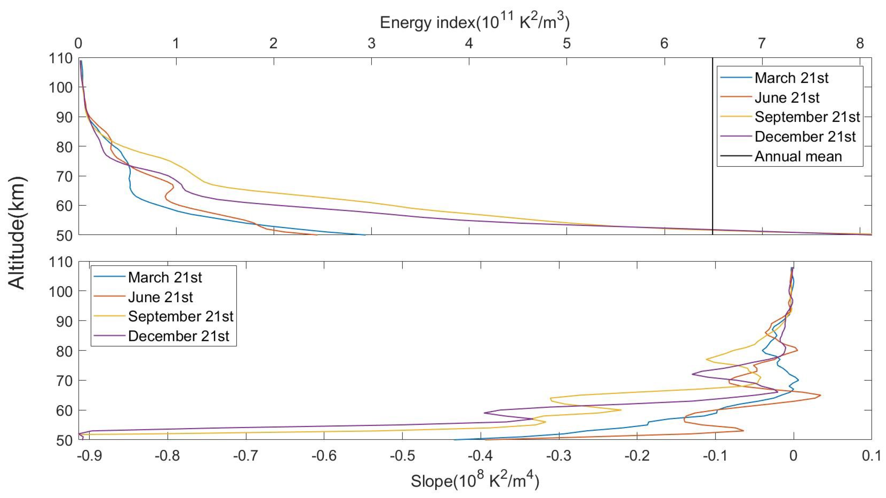
Figure 2 shows the energy index with height in the Beijing grid on 21 March, 21 June, 21 September, and 21 December 2006, respectively, as examples. First, we conducted a 5 km average on the original energy index data. This smoothing process served to filter out minor fluctuations that might have obscured significant trends in the energy index profile.
We mainly studied the change of energy index above the stratopause (50 km). As illustrated in Figure 2, several different decay processes of the energy index could be observed with increasing height. Initially, the profiles exhibited a notably rapid decay phase where turbulent dissipation played a dominant role. Then, there was a transition to a slower decaying phase. Finally, the energy index entered a very gradual decay phase, in which molecular dissipation became the primary dissipation mechanism.
We focused our investigation on variations of the energy index above the stratopause (50 km). As illustrated in Figure 2, the energy index exhibited several distinct decay processes with increasing altitude in this region. Each profile initially experienced a rapid decay phase characterized by the dominance of turbulent dissipation. Following this, there was a transition into a phase where the rate of decay began to slow down. Eventually, the profiles reached an extremely slow decay phase, in which molecular dissipation became the predominant factor. These three distinct sections of the energy index profile corresponded to three altitude bands, each exhibiting different patterns of temperature standard deviation with altitude.
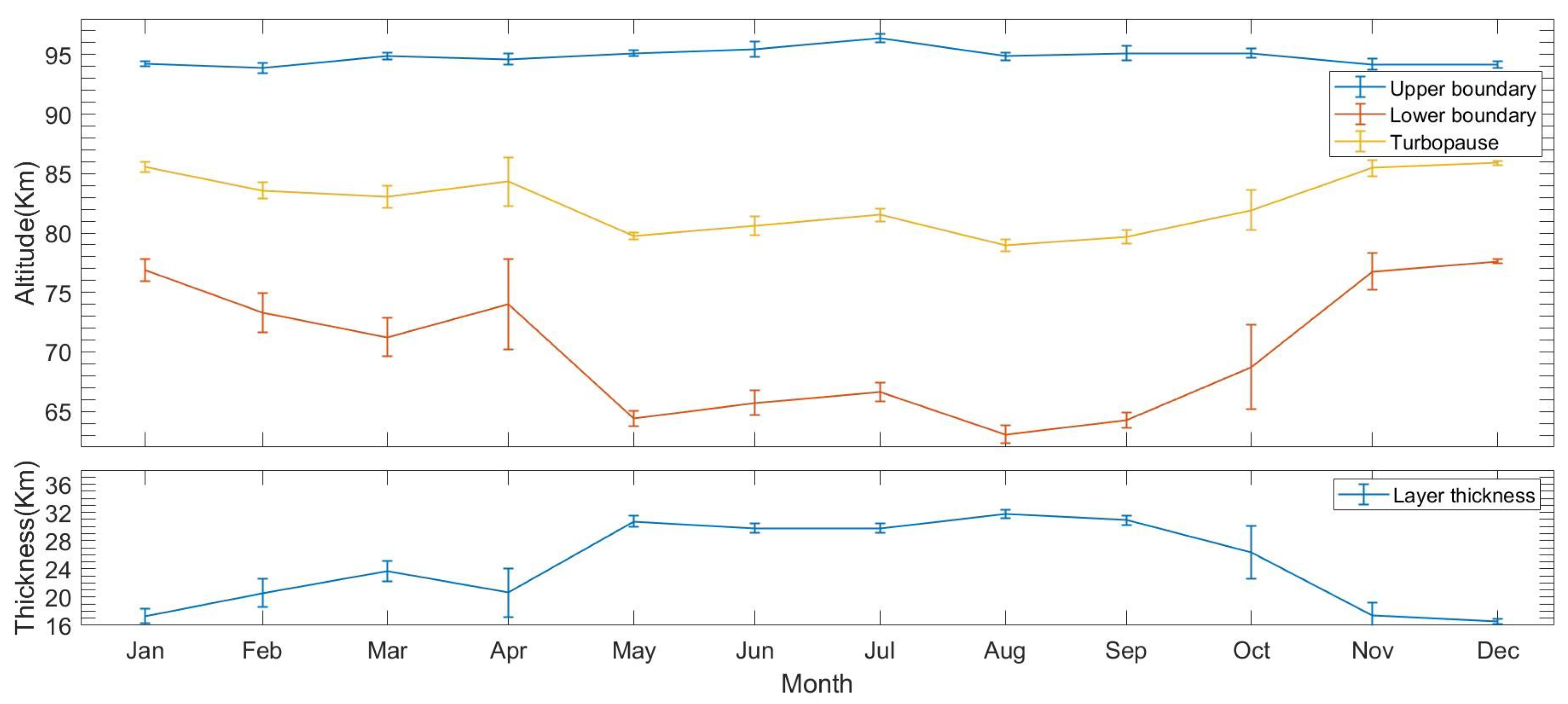
According to the observations presented in Figure 2, the upper boundary of the turbopause layer was defined at the altitude where molecular dissipation was fully dominant, marking the height where its influence became significantly pronounced. The lower boundary of the turbopause layer was set at the altitude where the inhibition of atmospheric wave activity by turbulence began to diminish. The turbopause was located in the turbopause layer, and its position was represented by the average of the upper and lower boundary positions. The thickness of the turbopause layer was the difference between the lower boundary and the upper boundary. Based on the vertical variation of the energy index C, the slope of which could be calculated, we differentiated the energy index by a central difference of 3 km to find the slope of the profile, as shown in Figure 2. This calculation enabled a detailed inspection of how the energy index evolved with altitude.
Each slope profile had similar characteristics. Initially, there was a rapid decay in the slope value until it reached a minimum point. Following this sharp decline, the slope began to increase again with altitude. Eventually, the slope stabilized, approaching a value close to zero at higher altitudes. The height at which the slope value started to be relatively stable and small was the height of the upper boundary of the turbopause layer.
The variation of the energy index with height within the range of 50 to 80 km could be classified into two distinct categories. The first type of energy index profile was smaller at 50 km, and there was a clear inflection point in the change with height, which may have been caused by the filtering of fluctuations by the summer wind. The second type of energy index profile was larger at 50 km, and there was no obvious inflection point in the altitude change. The annual average value of the energy index at 50 km was utilized to differentiate between these two profiles quantitatively. As shown in Figure 2, the average energy index at 50 km in 2009 was 6.92 · 10 11 K 2 / m 3 . The energy index profile on 21 March and 21 June was the first type of profile, and the profile on September 21st and December 21st was the second type of profile. Due to the inherent differences in characteristics between these profile types, it followed that the methodologies employed to determine the height of the lower boundary of the turbopause layer also had to vary accordingly.
For the first type of energy index profile, the presence of an inflection point with the energy index slope greater than 0 in the 50–60 km altitude band was a sign of this type of profile. This inflection point was interpreted as the altitude where atmospheric waves began to break up in significant quantities, due to wind filtration, indicating the onset of turbulence and energy dissipation processes.
In the context of the second type of energy index profile, the energy index exhibited a rapid decay, indicating a significant reduction in the energy available for atmospheric wave activity. This phenomenon was mainly related to turbulent activity, and the weakening of the inhibition effect of turbulence on atmospheric wave activity was mainly caused by the weakening of turbulence activity. Below 70 km, the atmosphere is generally regarded as being uniformly mixed [2]. This uniformity suggests higher levels of turbulent activity, as turbulent mixing tends to enhance the dispersal and dissipation of wave energy, so we needed to focus our analysis above 70 km. Since the characteristics are not obvious, we consider the lower boundary of the turbopause layer to be the location where the energy index began to be less than or equal to 1/e of the maximum energy index above 70 km.
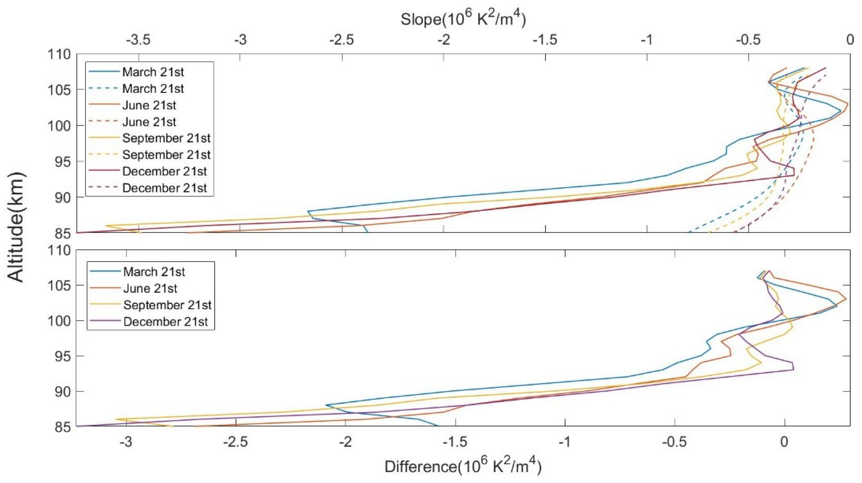
The upper boundary of the turbopause layer was the height at which the slope of the energy index began to maintain a small value. As illustrated in Figure 2, there was only a minor difference between the values of various energy indices around 90 km, but the slope value showed a downward trend in general. After reaching a certain height, the slope began to exhibit oscillatory behavior with height. To pinpoint the altitude at which this oscillation initiated, a linearly fitted slope profile was constructed that extended from various heights to the highest point of the energy index profile. This fitted profile is depicted as a dashed line in Figure 3. The following figure in Figure 3 shows how the difference between the two slope profiles obtained by different methods changed with height. The analysis revealed that the difference between the two slope profiles initially decreased with increasing height. However, as height continued to increase, this difference began to oscillate, displaying fluctuations around 0. The height at which the difference began to change from negative to positive was the height of the upper boundary of the turbopause layer.
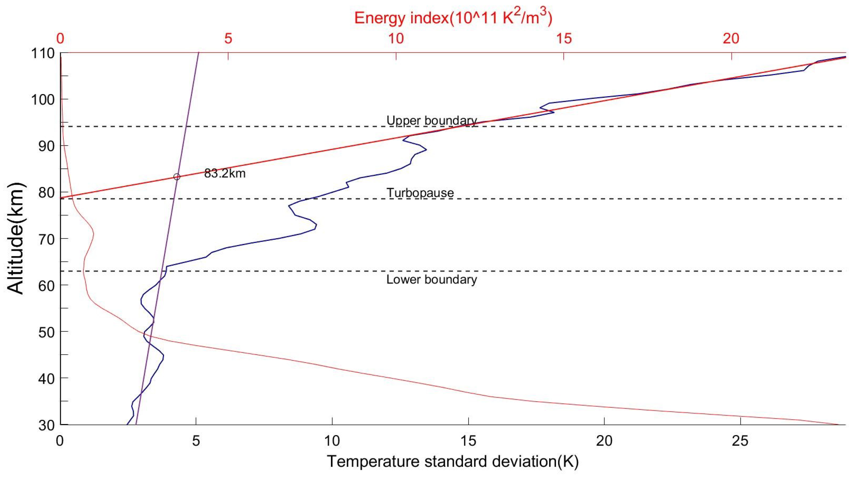
Figure 4 illustrates the variation of temperature standard deviation and the energy index with height, providing a comparative analysis of the two methods applied in our study. There is a very clear correspondence between the two profiles, suggesting the three different regions of variation of the energy index and the temperature standard deviation corresponded to each other. The region of the energy index profile that experienced a rapid decline corresponded to the lower portion of the temperature standard deviation profile, where the values increased linearly with height. The segment of the temperature standard deviation profile that marked the transition between the upper and lower boundaries of the turbopause was reflected in the energy index profile. The slow decreasing region of the energy index profile corresponded to the rapid increase observed at the upper portion of the temperature standard deviation profile.
A comparison between the traditional method and the new method for determining the turbopause reveals several key insights. Notably, the turbopause identified by the traditional method fell within the turbopause layer delineated by the new method. Above the upper boundary of this turbopause layer, the temperature standard deviation exhibited a relatively smooth variation with height, reflecting a more stable atmospheric profile. This observation emphasizes the significance of understanding the turbopause as a part of the transition zone. The traditional method primarily relies on linear wave theory, which provides valuable insight but may lack a description of the transition region. In contrast, the new method introduces a perspective based on energy conservation, which improves the traditional method by integrating variations in different profiles. Compared to traditional methods, the new method avoids relying on manual selection of segmentation regions for fitting.
By calculating a set of parameters, the new method expands the conventional view of the ‘turbopause’ to ‘turbopause layer’. This includes determining the upper and lower boundaries, the thickness of the turbopause layer, and the specific height of the turbopause itself. Importantly, this set of parameters aligns more closely with the intrinsic characteristics of the turbopause layer as a transitional region. It is also noteworthy that the turbopause height identified by the new method is computed as the average of the upper and lower boundaries. However, due to the exponential decrease in atmospheric density with height, the actual height of the turbopause is likely to be closer to the height of the upper boundary of the turbopause layer.

3. Result

3.1. Patterns of Change in Energy Index with Time–Altitude Variation

Using the methodology above, we calculated the energy index and several parameters associated with the turbopause layer of the Beijing grid (40° ± 2.5°, 120° ± 10°). The time–altitude distribution of the energy index is illustrated in Figure 5.
As illustrated in Figure 5, the energy index exhibited a downward trend with increasing altitude, characterized by an almost exponential decay that gradually slowed at higher elevations. This behavior can be attributed to the definition of the energy index, which was calculated as the product of the atmospheric density and the square of the temperature standard deviation. At lower altitudes, the influence of density reduction significantly outweighed relatively minor increases in atmospheric wave intensity, as indicated by the square of the temperature standard deviation. Consequently, the energy index experienced a pronounced exponential decline in this region. However, at higher altitudes the dynamic of the atmospheric waves changed. Here, the increase in the intensity of fluctuations became more pronounced, which offset the persistent decline in density and led to a moderation of the decline in the energy index. This suggests a significant seasonal variation in the energy index, as there are seasonal variations in both atmospheric waves and density.
Figure 6 illustrates that the main cycles of change in the energy index were different at different altitudes. In the range of 50–70 km, the cycle of energy indicators was dominated by the annual cycle, and the semi-annual cycle was weak. From 71 km and above, the semi-annual cycle started to strengthen. From 74 to 84 km, the semi-annual cycle was obvious, but the inter-annual cycle remained less distinct. Moreover, the distribution of cycles started to become chaotic, with some less distinct cycles appearing, especially around 89 km.
At altitudes around 85 km, the inter-annual cycle reasserted its dominance over other cycles, while the semi-annual cycle weakened considerably. From 89 km, the quasi-4-month cycle emerged as the most pronounced feature of the energy index, overshadowing both the annual and semi-annual cycles, which were both weak in this region. Additionally, near 89 km large-scale cycles were observed near this altitude, including variations spanning approximately 1.2 to 1.7 years, as well as phenomena associated with Quasi-Biennial Oscillation (QBO). From above 97 km, the quasi-4-month cycle became weaker and the energy index was dominated by the semi-annual cycle and the inter-annual cycle.

3.2. The Change of Parameters of Turbopause with Time

The monthly variations of the relevant parameters in the turbopause region, as calculated by the new method, are illustrated in Figure 7. From the data presented in Figure 7, it is clear that both the upper and lower boundaries of the turbopause layer exhibited significant inter-annual variability. Notably, the timing of the maximum and minimum values for these boundaries appeared to be inversely related. The upper boundary reached its minimum in December and its maximum in July, while the lower boundary exhibited its minimum in August and maximum in December. This pattern indicates a complex relationship between the thermal and dynamic processes within the turbopause layer region. Furthermore, there was evidence of semi-annual variations, particularly regarding the lower boundary, which peaked around February or March and again in August or September. Importantly, the amplitude of the seasonal variations was more pronounced for the lower boundary compared to the upper boundary. The mean values of the lower boundary and upper boundary were 69.17 km and 93.85 km, respectively.
Based on Figure 6, it appears that the larger values corresponding to both the upper and lower boundaries of the turbopause layer predominantly lie within the range of 70–80 km, aligning with a semi-annual variation in the energy index. The lower boundary values that were smaller typically occurred below 70 km, indicating an energy index that primarily demonstrated annual variability. The upper boundary values, on the other hand, were found within regions of more complex energy index variation cycles where the annual cycle did not dominate.
The position of the turbopause was obtained by averaging the upper boundary and the lower boundary, with an average of 81.51 km, so it also had very obvious seasonal characteristics. The thickness of the turbopause layer also had an obvious seasonal variation, but the phase was almost opposite to that of the lower boundary. This may be attributed to the relatively smaller inter-annual variation of the upper boundary compared to that of the lower boundary. This disparity suggests that the processes governing changes in these two layers are influenced by different factors and do not follow identical patterns.
The calculations also indicate that the error bars at the upper boundary were consistently smaller than those at the lower boundary. The error bar for the height of the upper boundary was relatively small in each month, indicating that the height variation of the upper boundary in each month was very small. The error bar of the height of the lower boundary was larger in spring and fall and smaller in summer and winter. The spring and autumn seasons were the transition seasons in which the proportion of the two types of energy index profiles changed in Figure 2, indicating that the factors affecting the energy index were relatively complex in these two seasons.
Figure 8 shows the results of the spectrum analysis of the upper boundary of the turbopause layer, the lower boundary of the turbopause layer, the position of the turbopause, and the thickness of the turbopause layer. As illustrated in Figure 8, the main cycle of variation for all parameters was the annual cycle. In addition to the inter-annual cycle, the lower boundary had a cycle of about 390 days, which may have been due to the splitting of the inter-annual cycle. It also had a distinct semi-annual cycle. The intensity of the semi-annual cycle was much lower than the intensity of the annual cycle. The upper boundary and the position of the turbopause also had periods of about 1.4–1.7 years, 2 years, and 3 years. This may have been related to atmospheric waves, and the energy index also had long periods near the upper boundary. In addition to these significant cycles, the upper and lower boundaries of the turbopause layer also had peaks near 120 days, but they were not significant.
The calculation of the Fourier transform shows that the amplitude of the annual cycle of the lower boundary was 5.81 km and the amplitude of the annual cycle of the upper boundary was 0.79 km, so it can be concluded that, as in Figure 7, the inter-annual variation of the lower boundary was stronger. And there were also different distributions between the significant cycles at the lower boundary and the significant cycles at the upper boundary. These indicate that the structure of atmospheric waves changes during the upward propagation process.
The findings of the study conducted by Offermann et al. [6] also pointed out that there is a significant seasonal variation in the turbopause at 40°N, which is higher in winter and summer and lower in fall and spring. They also illustrated that seasonal variation is annual at high latitudes and semi-annual at low latitudes and that there is a transition between the two at mid-latitudes. The reason for the kind of seasonal variation in the turbopause calculated by the traditional method may be that the turbopause is located between the upper and lower boundaries of the turbopause layer. The upper boundary is higher in summer and lower in winter, whereas the lower boundary has the opposite seasonal variation, and it is possible that the seasonal variation in the turbopause is due to a combination of factors affecting the upper boundary and factors affecting the lower boundary.

4. Discussion

The energy index is a comprehensive indicator of atmospheric waves, covering various types, such as tide, gravity waves, and planetary waves. However, it cannot distinguish between specific wave types. Atmospheric waves can be significantly modulated by prevailing wind fields. For example, gravity waves are filtered by these winds, which, in turn, affects the characteristics of the turbulent layer. To explore the influence of wind on the turbopause layer, we used zonal wind data obtained from the medium-frequency radar located in Langfang (39.4°N, 116.7°E). The analysis of the zonal wind data shown in Figure 9 indicates that there were significant inter-annual variations in winds at different altitudes. Specifically, the data indicated a distinct seasonal behavior in zonal wind between altitudes of 70 and 85 km. During the summer months, the zonal winds were predominantly directed eastward, while in the winter months they shifted to a westward orientation.
There was a strong correlation between the height of the lower boundary of the turbopause layer and the zonal wind. At 70 to 85 km, during periods when the zonal wind was directed eastward in this altitude range, the lower boundary of the turbopause layer was observed to drop. When the zonal wind was directed westward, the lower boundary of the turbopause layer rose. This relationship suggests that the behavior of the zonal wind plays a pivotal role in modulating the characteristics of the turbopause layer, likely due to the filtering effects exerted on gravity waves. Offermann et al. [6] also pointed out that the turbopause is found mainly near a zero-wind line or in regimes of low zonal wind speed, which is close to 85 km.
The mechanism behind this phenomenon may be related to the dynamics of gravity wave breaking, particularly in the summer months when significant wind reversal is noted at approximately 85 km. As gravity waves propagate upwards, if their phase velocity approaches the local wind speed, this can reduce the Richardson number, indicating the production of turbulence. Supporting these observations, Liu et al. [17] identified a persistent layer of enhanced gravity wave dissipation around the altitude range of 80 to 85 km. Mzé et al. [18] found that gravity wave dissipation is significantly more pronounced above 70 km compared to lower altitudes throughout all seasons. This increased rate of dissipation in the summer months is likely related to the wind inversion seen at 85 km, which can encourage gravity wave breaking and subsequent turbulence production.
As atmospheric waves propagate upward, when these waves reach a critical threshold of instability, they break, resulting in turbulence [19]. This breaking process not only generates turbulence but also plays a role in determining the position of the turbopause, so the intensity and characteristics of the atmospheric waves influence the turbopause layer. Moreover, the energy index of atmospheric waves exhibits distinct periodic changes at varying altitudes. These variations can be interpreted as reflecting shifts in the composition and structure of the atmospheric waves as they ascend through different layers of the atmosphere.
At mid-latitudes, atmospheric dynamics is significantly influenced by gravity waves and quasi-2-day waves, particularly at altitudes below 70 km, where their amplitudes are dominant. Both types of waves exhibit strong annual variations, which can profoundly affect atmospheric behavior and stability [20]. As gravity waves ascend and reach altitudes above 70 km, they can become unstable. Mzé et al. [18] employed Rayleigh radar techniques to investigate the vertical distribution of potential energy associated with gravity waves in the mid-northern latitudes. They found an inter-annual variation at the bottom of the mesosphere and found a semi-annual cycle at about 75 km.
In the altitude range of 88 to 98 km, Tian et al. [21] found that gravity fluctuation fluxes with periods of less than 2 h show seasonal variations in the middle atmosphere (MLT) region at 40°N. They observed that easterly momentum variations show a clear inter-Annual Oscillation (AO), while at the bottom and top of the MLT region there is the effect of the Semi-Annual Oscillation (SAO). Meanwhile, close to 95 km altitude, the study also found a quasi-4-month oscillation. On the other hand, the meridional momentum flux is characterized by strong inter-annual oscillations below 95 km, while above 92 km it exhibits weak Semi-Annual Oscillations, and a quasi-4-month oscillation was also observed above 95 km. In addition, Huang et al. [22] showed that 6.5 DW with a period of quasi-4-month is also very obvious in the middle atmosphere region, and the effect is especially significant in the northern hemisphere region. Gong et al. [23], on the other hand, pointed out that the amplitude of Triangular Oscillation (TAO) is as important as AO and SAO in the middle atmosphere region, which further emphasizes the relative importance of the multiple modes of oscillation in the dynamics of the MLT region.
The study of atmospheric tides, particularly in the MLT region, indicates that their amplitudes become increasingly noticeable at altitudes above approximately 98 km. Research indicates that at mid-latitudes, the amplitude of the semi-diurnal tide often exceeds that of the diurnal tide [24]. Yu et al. [25] further elucidated this phenomenon by highlighting the presence of a clear SAO within the diurnal tides. In the semi-diurnal component, SAO dominates the low-latitude stations. However, at mid-latitudes, AO becomes more pronounced. Moreover, around the altitude of 100 km, the diurnal tide experiences breaking, leading to a transition where the semi-diurnal tide becomes the primary influence, resulting in the energy index being mainly inter-annual and semi-annual changes.
At 78 to 100 km, the period of the energy index becomes very complex, and this property could be caused by the combination of planetary waves, tides, gravity waves and their interactions, probably mainly gravity waves and planetary waves. In this region, there may be no obvious dominant fluctuations, and the intensity of various atmospheric fluctuations is small, which will be coupled with different periodic changes.
Atmospheric turbulence is often associated with atmospheric waves, and there have been many studies on the relationship between atmospheric waves and turbulent activity, with the majority of studies focusing on atmospheric gravity waves and atmospheric turbulent activity [26,27], but there have also been carried out on the relationship between atmospheric turbulent activity and tides [5] or planetary waves [16]. Ge et al. [16] mentioned that there is a connection between turbopause calculated using traditional methods and the 6.5 DW. Since we did not calculate the specific value of a wave, the results from the Beijing area show that gravity waves may have a greater influence on the changes of the lower boundary of the turbopause layer. Some gravity waves with short vertical wavelengths will break up in the process of upward propagation, and there will be a half-year change of gravity waves around 75 km.
In addition, the turbopause is usually located in the altitude range of about 78 to 93 km. Around this height, there are significant interactions between the various atmospheric waves. The main waves are likely to be gravity waves and planetary waves, which play an important role in the atmosphere. As a transition region, the turbopause layer is not only an interface between the troposphere and the outer atmosphere, but also a place where various atmospheric fluctuations and dynamic activities converge. Within the turbulent layer, complex atmospheric wave interactions occur frequently. These waves interact with each other, leading to significant changes in the behavior of waves in the atmosphere. For example, gravity waves are affected by planetary waves and vice versa.

5. Conclusions

In this paper, we propose a novel method for determining the height of the turbopause, using SABER/TIMED temperature data and number density data. This method addresses the limitations of traditional linear fitting techniques, which often introduce subjectivity and uncertainty due to variances in regional data selection and fitting procedures. We also introduce a new set of parameters to characterize the turbopause more comprehensively. The methodology focuses on the identification of both the upper and lower boundaries of the turbopause layer, which can be defined by analyzing changes in the energy index, which is a quantitative measure of atmospheric wave activity. Both the upper and lower boundaries of the turbopause layer exhibit significant inter-annual variability. Notably, the phases of these two boundaries are inversely correlated, which means that when one boundary rises, the other tends to fall. Furthermore, we observe that the amplitude of the inter-annual cycle for the lower boundary is greater than that of the upper boundary.
Both the wind speed and the intensity of the atmospheric wave affect the position of the turbopause. Wind speed plays a vital role in this dynamic because it influences the behavior and propagation of atmospheric waves. These interactions can modify the vertical structure of the atmosphere and, consequently, impact the height at which the turbopause is located. The energy of the waves in the atmosphere can be quantified using an energy index, which serves as a tool to represent the intensity and characteristics of atmospheric waves. This index exhibits varying periodic changes at different altitudes, and this change can represent the dominant wave in the atmospheric wave, to some extent. The cycle of variation of the energy index at different altitudes is predominantly annual. However, two altitude segments are not predominantly annual, and the upper and lower boundaries of the turbopause layer are also related to these two height regions. Furthermore, the periodic variation of the parameters of the turbopause layer is also dominated by annual variation.
Gravity waves play an important role in atmospheric dynamics at lower altitudes. From approximately 50 km upward, gravity waves start to break, a phenomenon that occurs when the waves transfer energy to the surrounding atmosphere, creating turbulence and promoting mixing. At an altitude of about 90 km, another important atmospheric wave, the tides, begins to become more and more pronounced. Moreover, the intensity of the planetary waves changes with increasing altitude, and the proportion of the total energy of the atmospheric waves accounted for by these waves changes at different altitudes.
The turbopause—which represents a transitional layer in the atmosphere where the composition of air begins to change significantly, due to the influence of molecular diffusion and atmospheric wave activity—plays a significant role in various fields, including atmospheric weather modeling, climate studies, and environmental monitoring. In our next study, we plan to apply the newly developed method to the SABER/TIMED data set on a global scale. The results of the study could provide valuable information for understanding the spatial and temporal characteristics of the turbopause layer. A dataset documenting the characteristics of the turbopause layer will also be available, which can be used directly in modeling the middle and upper atmosphere.

Author Contributions

Conceptualization, C.X.; methodology, C.X. and Z.W.; software, Z.W.; validation, Z.W., C.X., X.H., J.Y. and X.C.; formal analysis, Z.W.; investigation, C.X. and Z.W.; resources, X.H., J.Y., X.C. and K.L.; writing—original draft preparation, Z.W.; writing—review and editing, Z.W., C.X., L.X., X.W., Y.Y. and H.L.; visualization, Z.W.; supervision, C.X.; project administration, C.X.; funding acquisition, C.X. All authors have read and agreed to the published version of the manuscript.

Funding

This research is funded by the National Natural Science Foundation of China (NSFC) Grant No.12241101, 42174192, 91952111.

Data Availability Statement

The original contributions presented in this study are included in the article. Further inquiries can be directed to the corresponding author.

Acknowledgments

Thanks to the team of SABER/TIMED for supporting data, which are public and available at https://saber.gats-inc.com/.

Conflicts of Interest

The authors declare no conflicts of interest.

References

  1. Hall, C.M.; Holmen, S.E.; Meek, C.E.; Manson, A.H.; Nozawa, S. Change in turbopause altitude at 52 and 70 N. Atmos. Chem. Phys. 2016, 16, 2299–2308. [Google Scholar] [CrossRef]
  2. Emmert, J.T.; Drob, D.P.; Picone, J.M.; Siskind, D.E.; Jones, M.; Mlynczak, M.G.; Bernath, P.F.; Chu, X.; Doornbos, E.; Funke, B.; et al. NRLMSIS 2.0: A whole-atmosphere empirical model of temperature and neutral species densities. Earth Space Sci. 2021, 8, e2020EA001321. [Google Scholar] [CrossRef]
  3. Lehmacher, G.A.; Larsen, M.F.; Collins, R.L.; Barjatya, A.; Strelnikov, B. On the short-term variability of turbulence and temperature in the winter mesosphere. Ann. Geophys. 2018, 36, 1099–1116. [Google Scholar] [CrossRef]
  4. Roper, R.; Berkey, F. Mesospheric and lower thermospheric turbulence over Bear Lake, Utah, 1999–2003. J. Atmos. Sol.-Terr. Phys. 2011, 73, 921–924. [Google Scholar] [CrossRef]
  5. Wang, Z.; Xiao, C.; Hu, X.; Yang, J.; Cheng, X.; Xu, Q.; Xiao, L.; Wu, X. Short-Period Variation of the Activity of Atmospheric Turbulence in the MLT Region over Langfang. Atmosphere 2023, 14, 1045. [Google Scholar] [CrossRef]
  6. Offermann, D.; Jarisch, M.; Schmidt, H.; Oberheide, J.; Grossmann, K.; Gusev, O.; Russell III, J.; Mlynczak, M. The “wave turbopause”. J. Atmos. Sol.-Terr. Phys. 2007, 69, 2139–2158. [Google Scholar] [CrossRef]
  7. John, S.R.; Kumar, K.K. The concept of wave-turbopause layer and its signature in the global mesosphere-lower thermospheric gravity wave activity: CONCEPT OF WAVE-TURBOPAUSE LAYER. J. Geophys. Res. 2012, 117, A10310. [Google Scholar] [CrossRef]
  8. Lehmacher, G.A.; Scott, T.D.; Larsen, M.F.; Bilén, S.G.; Croskey, C.L.; Mitchell, J.D.; Rapp, M.; Lübken, F.J.; Collins, R.L. The Turbopause experiment: Atmospheric stability and turbulent structure spanning the turbopause altitude. Ann. Geophys. 2011, 29, 2327–2339. [Google Scholar] [CrossRef]
  9. Offermann, D.; Jarisch, M.; Oberheide, J.; Gusev, O.; Wohltmann, I.; Russell, J.; Mlynczak, M. Global wave activity from upper stratosphere to lower thermosphere: A new turbopause concept. J. Atmos. Sol.-Terr. Phys. 2006, 68, 1709–1729. [Google Scholar] [CrossRef]
  10. Zhao, X.R.; Sheng, Z.; Li, J.W.; Yu, H.; Wei, K.J. Determination of the “Wave Turbopause” Using a Numerical Differentiation Method. J. Geophys. Res. Atmos. 2019, 124, 10592–10607. [Google Scholar] [CrossRef]
  11. Russell, J.M., III; Mlynczak, M.G.; Gordley, L.L.; Tansock, J.J., Jr.; Esplin, R.W. Overview of the SABER experiment and preliminary calibration results. In Proceedings of the SPIE’s International Symposium on Optical Science, Engineering, and Instrumentation, Denver, CO, USA, 18–23 July 1999; Larar, A.M., Ed.; p. 277. [Google Scholar] [CrossRef]
  12. Mertens, C.J.; Mlynczak, M.G.; López-Puertas, M.; Wintersteiner, P.P.; Picard, R.H.; Winick, J.R.; Gordley, L.L.; Russell, J.M. Retrieval of mesospheric and lower thermospheric kinetic temperature from measurements of CO 2 15 µm Earth Limb Emission under non-LTE conditions. Geophys. Res. Lett. 2001, 28, 1391–1394. [Google Scholar] [CrossRef]
  13. Xiao, C.; Hu, X.; Tian, J. Global temperature stationary planetary waves extending from 20 to 120 km observed by TIMED/SABER. J. Geophys. Res. 2009, 114, D17101. [Google Scholar] [CrossRef]
  14. Cheng, X.; Yang, J.; Xiao, C.; Hu, X. Density Correction of NRLMSISE-00 in the Middle Atmosphere (20–100 km) Based on TIMED/SABER Density Data. Atmosphere 2020, 11, 341. [Google Scholar] [CrossRef]
  15. Offermann, D.; Gusev, O.; Donner, M.; Forbes, J.M.; Hagan, M.; Mlynczak, M.G.; Oberheide, J.; Preusse, P.; Schmidt, H.; Russell, J.M. Relative intensities of middle atmosphere waves. J. Geophys. Res. 2009, 114, D06110. [Google Scholar] [CrossRef]
  16. Ge, W.; Sheng, Z.; Huang, Y.; He, Y.; Liao, Q.; Chang, S. Different Influences on “Wave Turbopause” Exerted by 6.5 DWs and Gravity Waves. Remote Sens. 2023, 15, 800. [Google Scholar] [CrossRef]
  17. Liu, X.; Xu, J.; Yue, J.; Kogure, M. Persistent Layers of Enhanced Gravity Wave Dissipation in the Upper Mesosphere Revealed From SABER Observations. Geophys. Res. Lett. 2022, 49. [Google Scholar] [CrossRef]
  18. Mzé, N.; Hauchecorne, A.; Keckhut, P.; Thétis, M. Vertical distribution of gravity wave potential energy from long-term Rayleigh lidar data at a northern middle-latitude site. JGR Atmos. 2014, 119. [Google Scholar] [CrossRef]
  19. Fritts, D.C.; Alexander, M.J. Gravity wave dynamics and effects in the middle atmosphere. Rev. Geophys. 2003, 41, 1003. [Google Scholar] [CrossRef]
  20. Namboothiri, S.P.; Kishore, P.; Igarashi, K. Observations of the quasi-2-day wave in the mesosphere and lower thermosphere over Yamagawa and Wakkanai. J. Geophys. Res. 2002, 107, ACL 13-1–ACL 13-13. [Google Scholar] [CrossRef]
  21. Tian, C.; Hu, X.; Liu, Y.; Cheng, X.; Yan, Z.; Cai, B. Seasonal Variations of High-Frequency Gravity Wave Momentum Fluxes and Their Forcing toward Zonal Winds in the Mesosphere and Lower Thermosphere over Langfang, China (39.4 N, 116.7 E). Atmosphere 2020, 11, 1253. [Google Scholar] [CrossRef]
  22. Huang, Y.Y.; Zhang, S.D.; Li, C.Y.; Li, H.J.; Huang, K.M.; Huang, C.M. Annual and interannual variations in global 6.5 DWs from 20 to 110 km during 2002–2016 observed by TIMED/SABER: Long-Term Variations of 6.5 DWs. J. Geophys. Res. Space Phys. 2017, 122, 8985–9002. [Google Scholar] [CrossRef]
  23. Gong, Y.; Li, C.; Ma, Z.; Zhang, S.; Zhou, Q.; Huang, C.; Huang, K.; Li, G.; Ning, B. Study of the Quasi-5-Day Wave in the MLT Region by a Meteor Radar Chain. JGR Atmos. 2018, 123, 9474–9487. [Google Scholar] [CrossRef]
  24. Igarashi, K.; Namboothiri, S.; Kishore, P. Tidal structure and variability in the mesosphere and lower thermosphere over Yamagawa and Wakkanai. J. Atmos. Sol.-Terr. Phys. 2002, 64, 1037–1053. [Google Scholar] [CrossRef]
  25. Yu, Y.; Wan, W.; Ren, Z.; Xiong, B.; Zhang, Y.; Hu, L.; Ning, B.; Liu, L. Seasonal variations of MLT tides revealed by a meteor radar chain based on Hough mode decomposition. JGR Space Phys. 2015, 120, 7030–7048. [Google Scholar] [CrossRef]
  26. Guo, Y.; Liu, A.Z.; Gardner, C.S. First Na lidar measurements of turbulence heat flux, thermal diffusivity, and energy dissipation rate in the mesopause region. Geophys. Res. Lett. 2017, 44, 5782–5790. [Google Scholar] [CrossRef]
  27. Sedlak, R.; Hannawald, P.; Schmidt, C.; Wüst, S.; Bittner, M.; Stanič, S. Gravity wave instability structures and turbulence from more than 1.5 years of OH* airglow imager observations in Slovenia. Atmos. Meas. Tech. 2021, 14, 6821–6833. [Google Scholar] [CrossRef]
Figure 1. The picture on the right is the daily mean temperature profile at 40°N on 15 September 2002, and the picture on the left is the temperature standard deviation profile and fitted lines for different height segments. The solid black line shows the temperature standard deviation for the 40°N latitude circle and the dashed black line shows the temperature standard deviation for the Beijing grid (40° ± 2.5°, 120° ± 10°). The colored lines represent the results of fitting the standard deviation of the temperature of the latitude circle at 40°N with different altitude segments.
Remotesensing 17 00623 g001
Figure 2. Energy index and its slope change with the height of the Beijing grid on 21 March, 21 June, 21 September, and 15 December 2006 for different colors. The black line represents the annual average at 50 km of the energy index.
Remotesensing 17 00623 g002
Figure 3. In the graph above, the solid line represents the slope of the energy index, and the dashed line represents the fit slope of the energy index from its current height to its apex. The chart below shows the difference between the two.
Remotesensing 17 00623 g003
Figure 4. Temperature standard deviation(blue) and energy index(red) change with height on 15 September 2002. The two colored straight lines are fitted to 30–65 km and 91–110 km, respectively.
Remotesensing 17 00623 g004
Figure 5. The energy index of the Beijing grid varied with season and height.
Remotesensing 17 00623 g005
Figure 6. Normalized spectral graphs of energy indices at different altitudes. The black lines represent areas with confidence levels above 0.99.
Remotesensing 17 00623 g006
Figure 7. The position of the upper boundary of the turbopause layer, the position of the lower boundary of the turbopause layer, the position of turbopause, and the thickness of the turbopause layer change with months. The values for each month are the average of approximately 21 years for each month.
Remotesensing 17 00623 g007
Figure 8. Lomb–Scargle diagram of the upper boundary of the turbopause layer, the lower boundary of the turbopause layer, and the position of the turbopause. These straight lines represent their respective positions with 99% confidence.
Remotesensing 17 00623 g008
Figure 9. Variation of zonal wind with height and season. The black line means the zonal wind is zero. The red line represents the upper boundary and the blue line represents the lower boundary.
Remotesensing 17 00623 g009
Disclaimer/Publisher’s Note: The statements, opinions and data contained in all publications are solely those of the individual author(s) and contributor(s) and not of MDPI and/or the editor(s). MDPI and/or the editor(s) disclaim responsibility for any injury to people or property resulting from any ideas, methods, instructions or products referred to in the content.

