
Leveraging Ice, Cloud, and Land Elevation Satellite-2 Laser Altimetry and Surface Water Ocean Topography Radar Altimetry for Error Diagnosis in Hydraulic Models: A Case Study of the Chao Phraya River


Abstract
1. Introduction
2. Materials
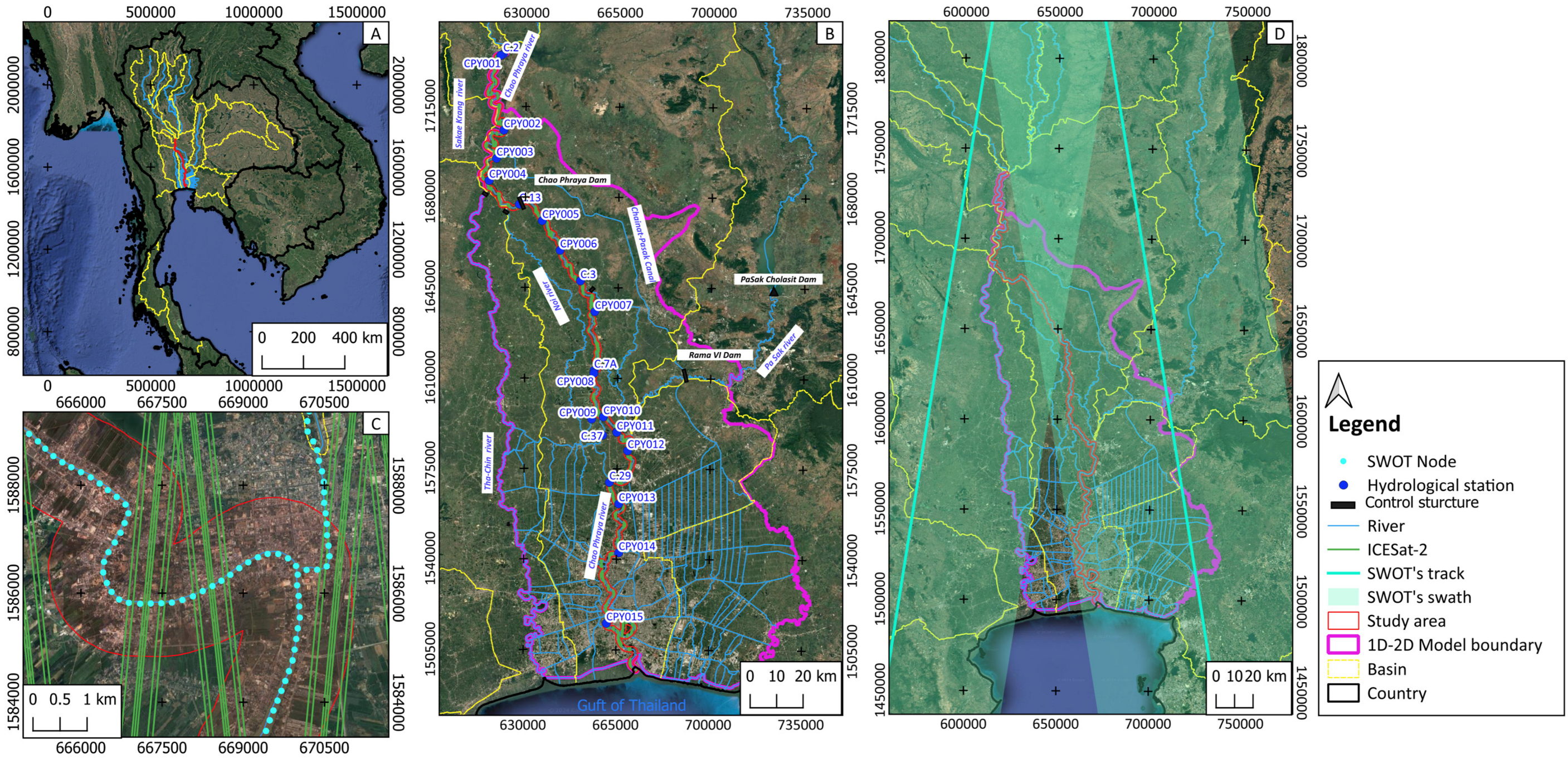
2.1. Study Area
2.2. Hydraulic Model
2.3. ICESat-2 Satellite Laser Altimetry
- ATL03: ATLAS/ICESat-2 L2A Global Geolocated Photon Data
- ATL13: ATLAS/ICESat-2 L3A Inland Water Surface Height
2.4. Surface Water and Ocean Topography (SWOT) Satellite
2.5. Water Mask
2.6. In Situ Data
3. Methods
3.1. Hydraulic Modeling Setup
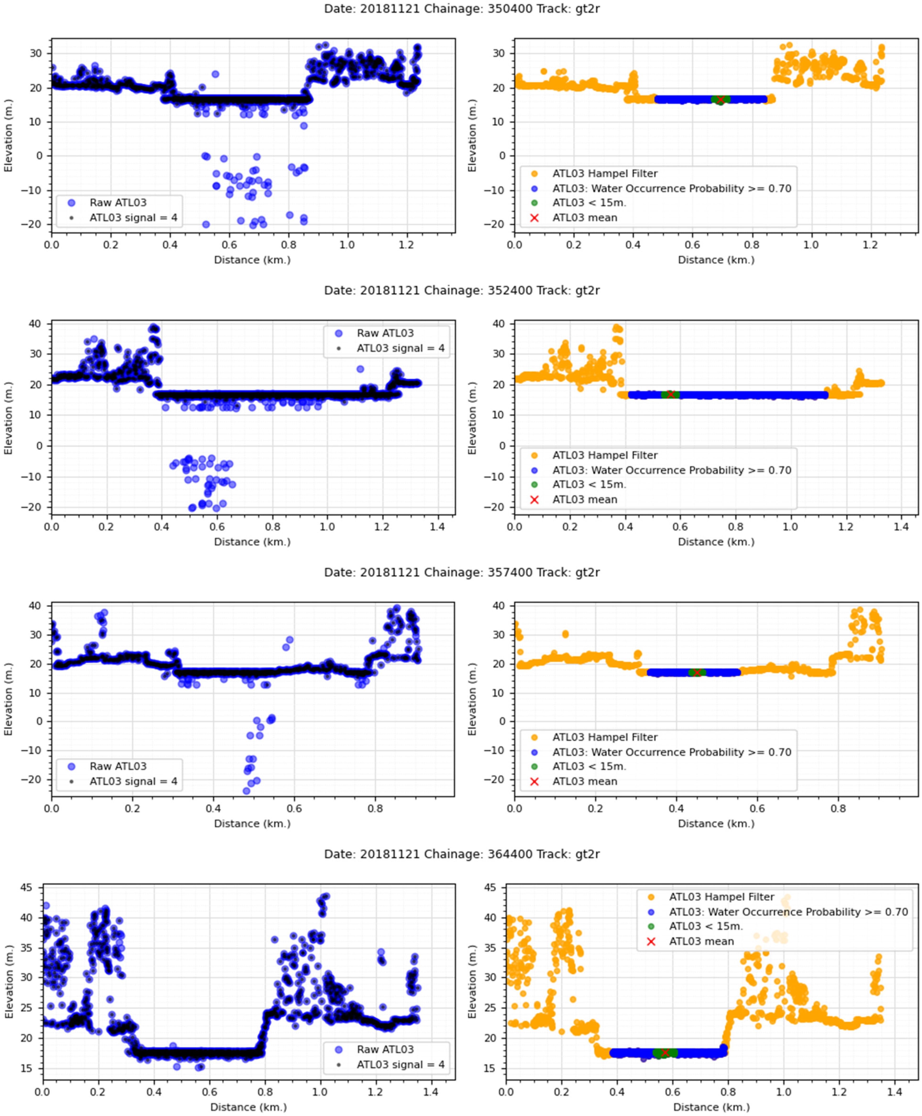
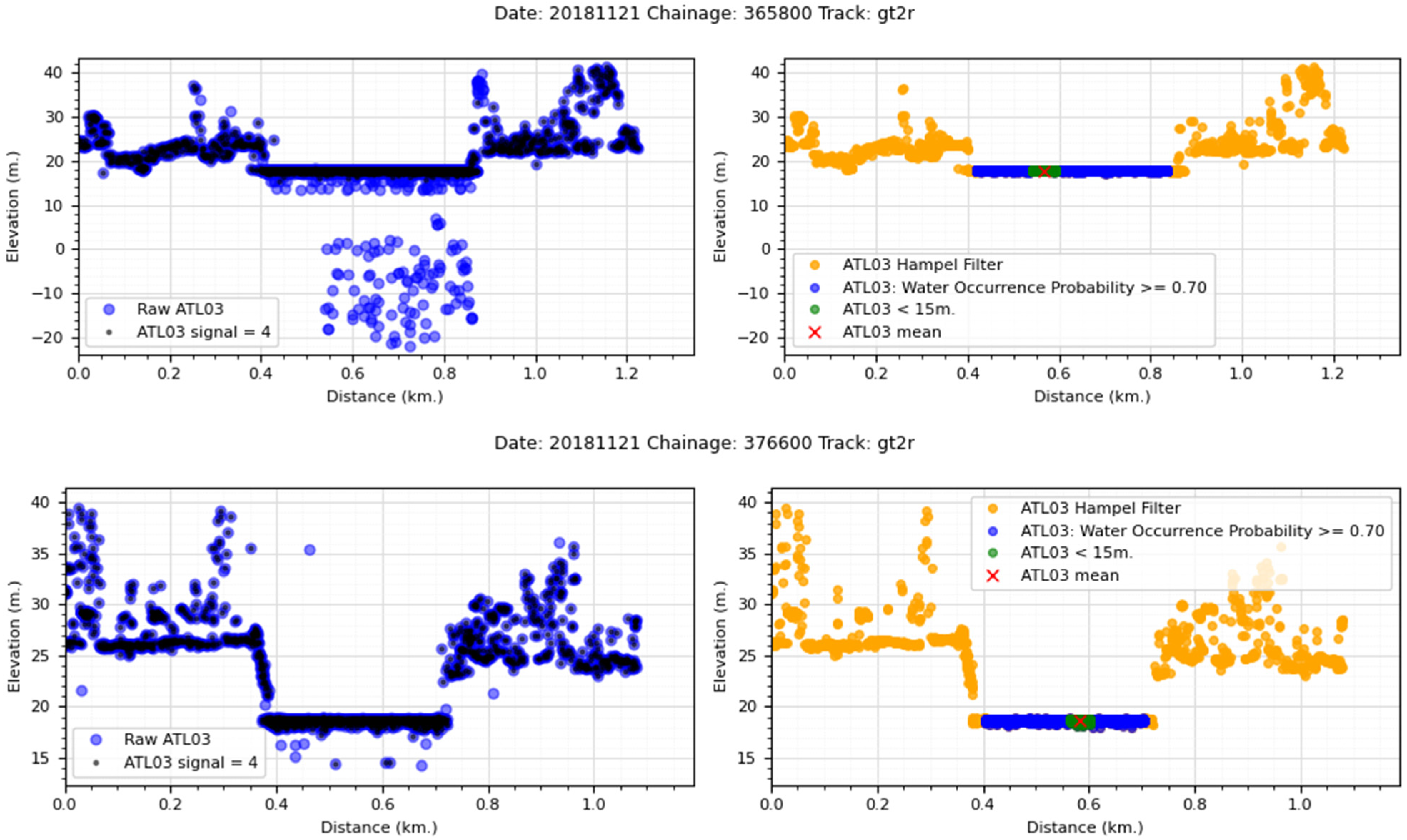
3.2. ICESat-2 ATL03 Data Processing
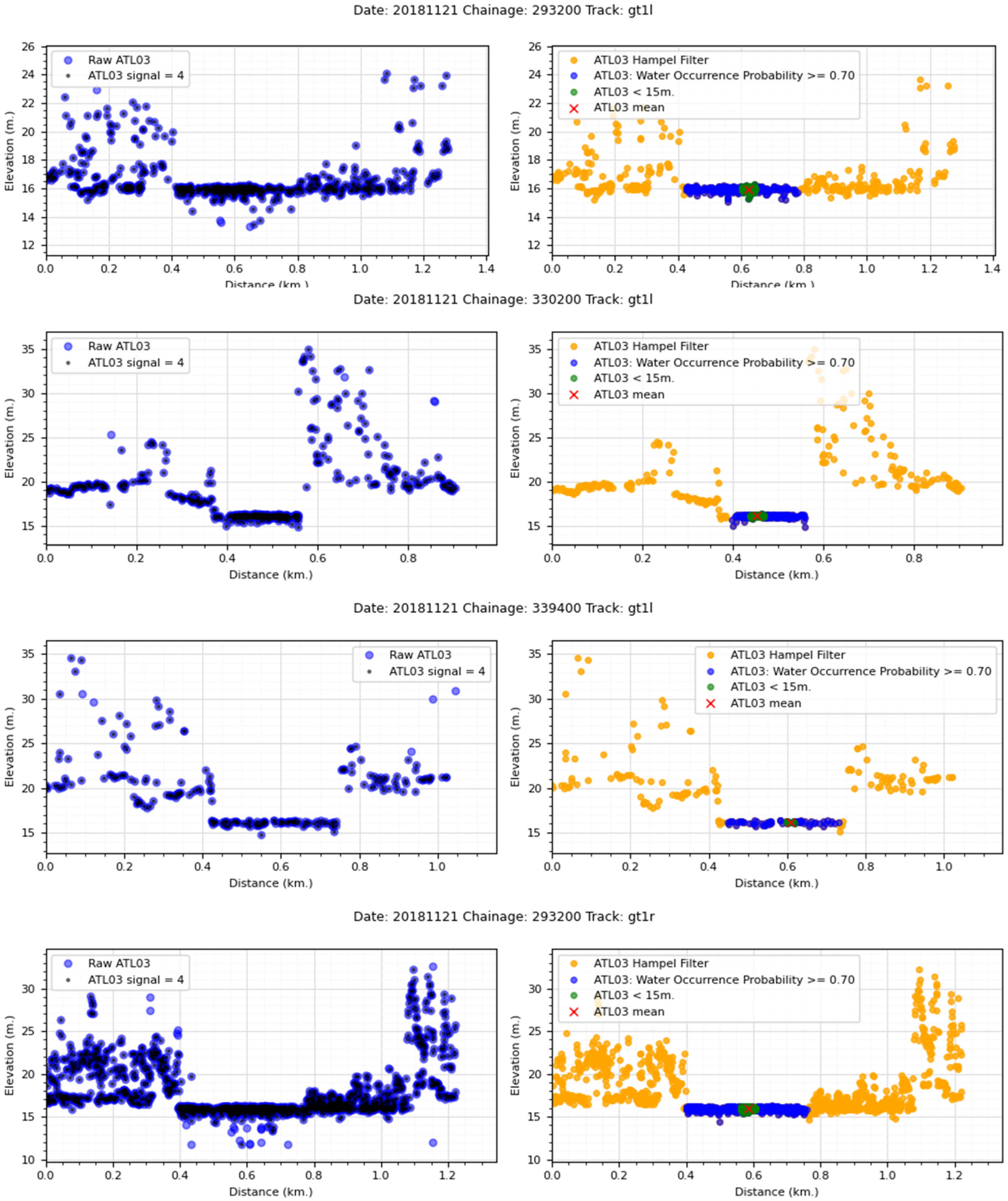
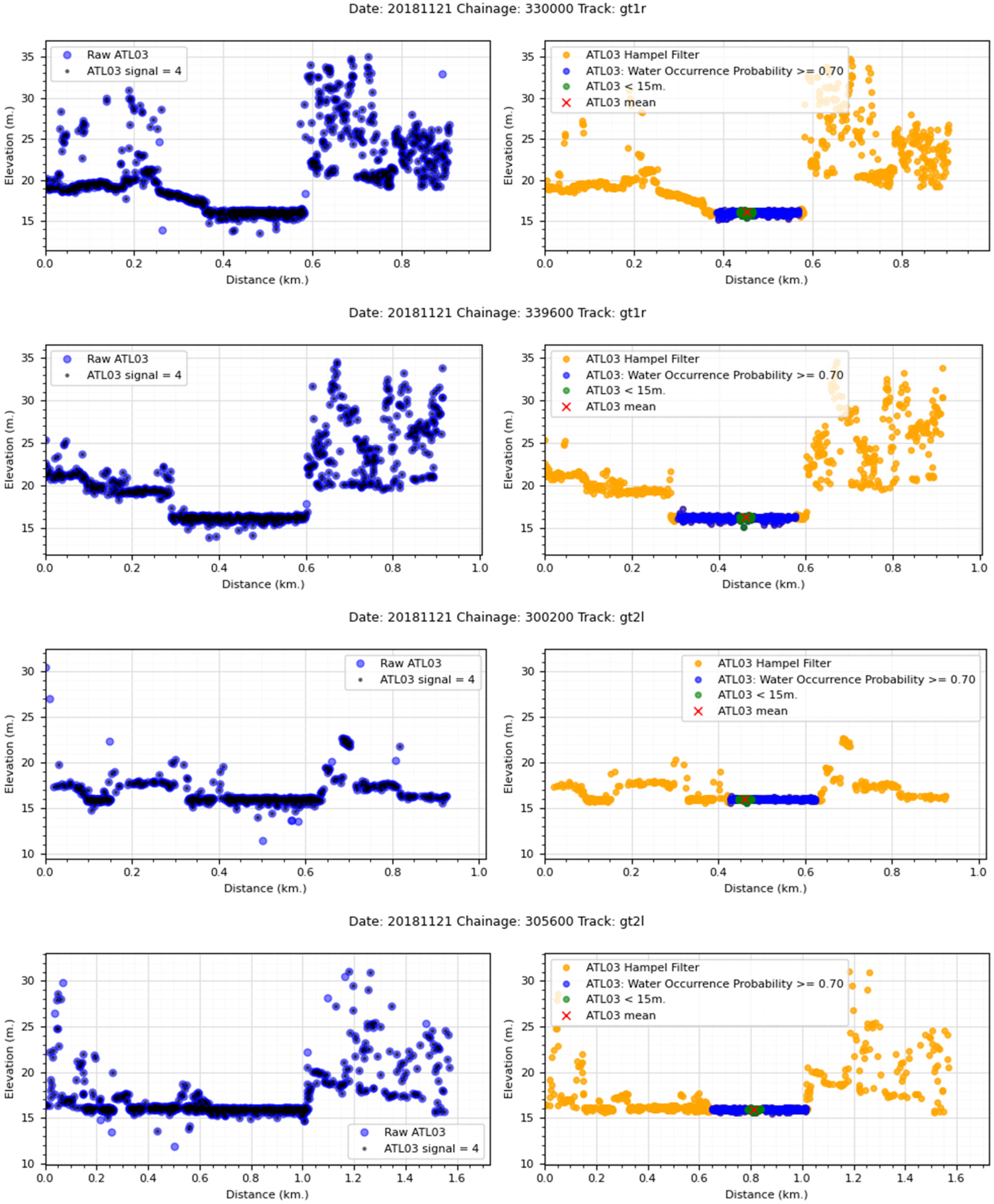
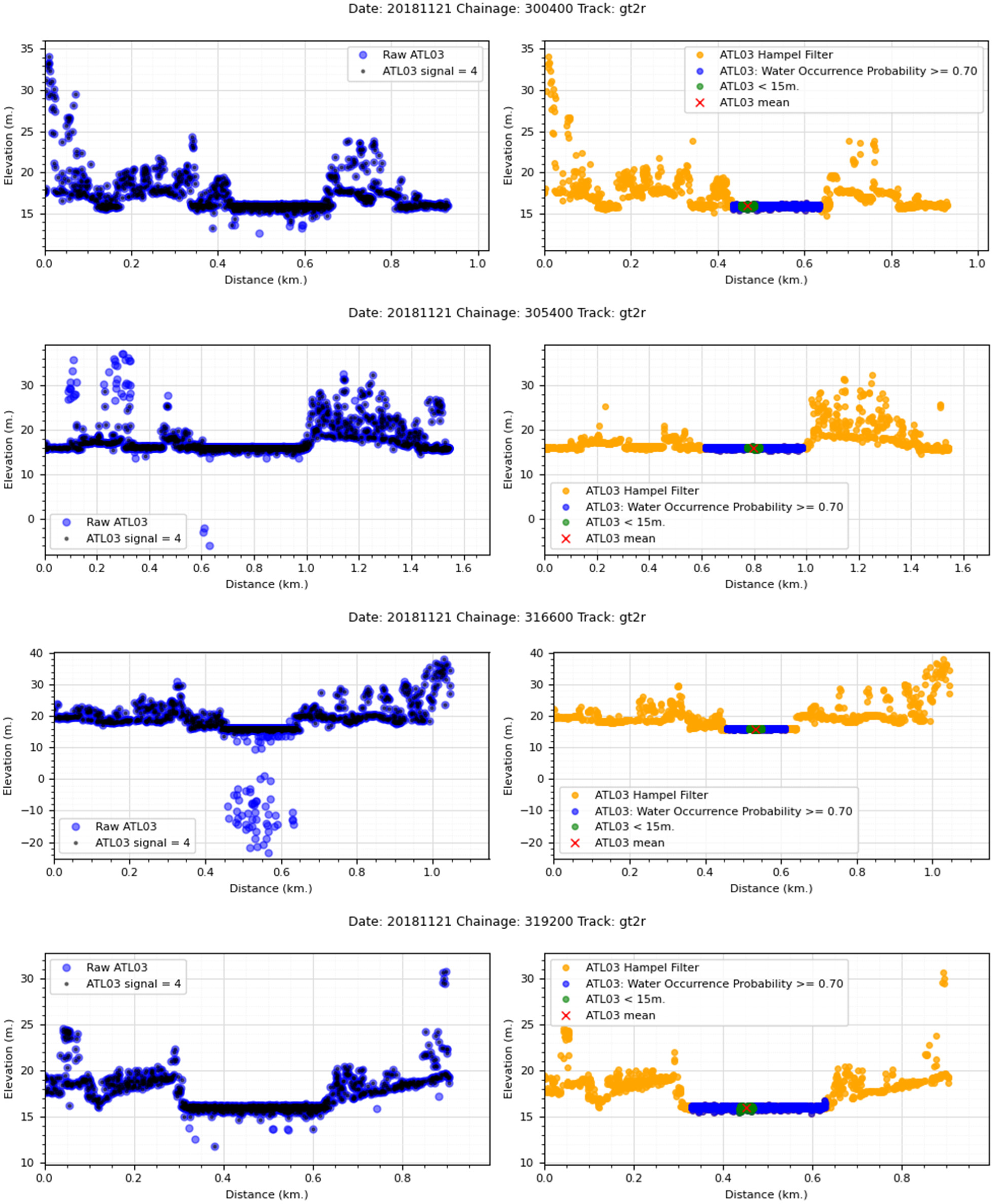
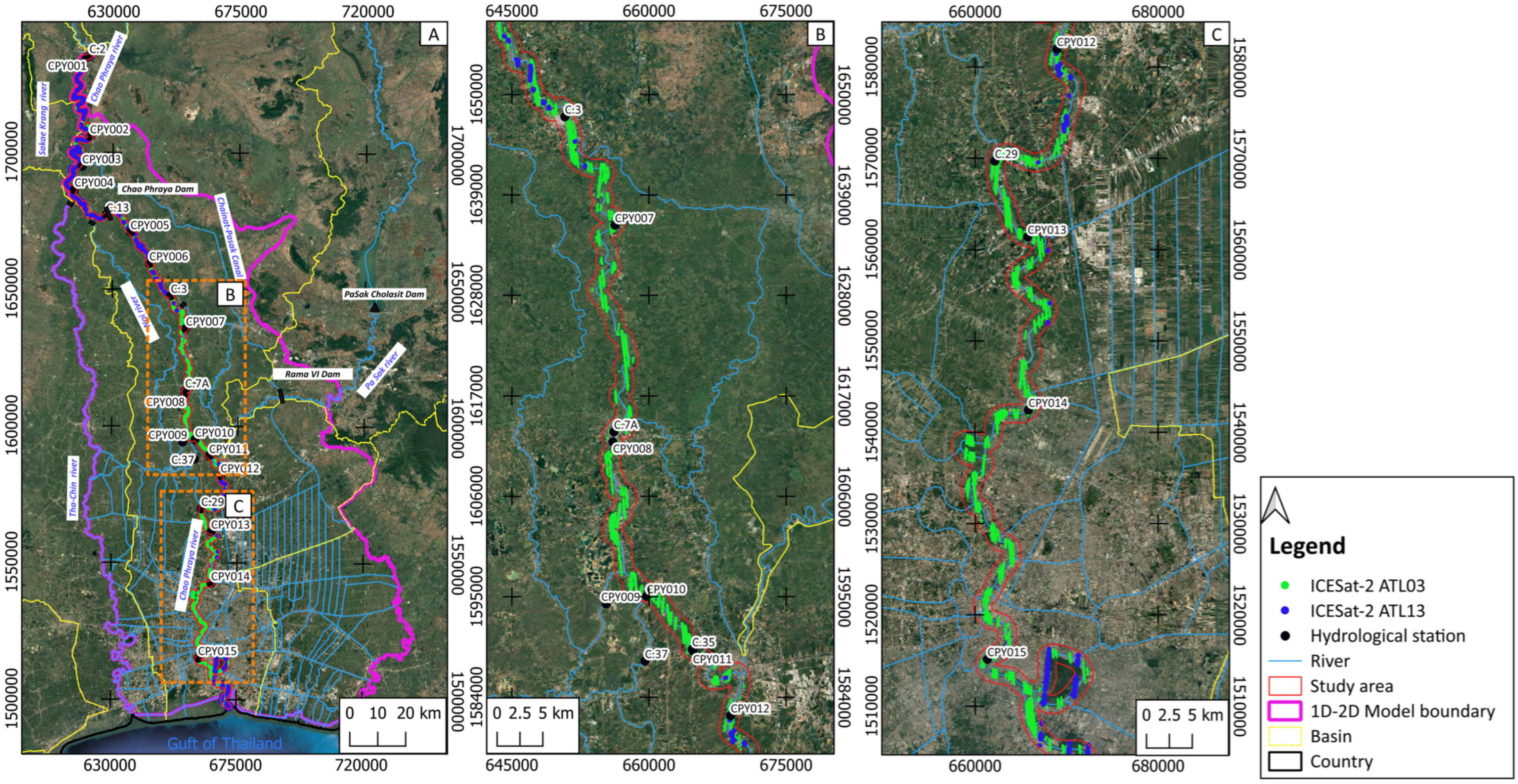
- ▪ The ICESat-2 ATL03 data were processed to extract the following parameters: latitude (Lat_ph), longitude (Long_ph), height (h_ph) relative to the WGS84 ellipsoid, photon signal confidence (signal_conf_ph), and time (delta_time) in Coordinated Universal Time (UTC). To ensure data accuracy and relevance, only measurements within a 1-kilometer distance from the CPY river’s centerline were considered, as shown in Figure 6A.
- ▪ To evaluate WSE, it is necessary to use the same vertical datum reference. In this study, the vertical datum reference used was TGM2017 [40] to standardize the datum, which provides the best fit for Thailand. Equation (1) was used to establish accurate measurements of vertical elevation.
- ▪ Subsequently, chainage points for the ICESat-2 ATL03 product were assigned following the same convention as the hydraulic model to ensure consistency. The ATL03 photons were filtered using the photon signal confidence (signal_conf_ph) parameter, which categorizes confidence levels into three groups: high (4), medium (3), and low (2) confidence. In this study, only ATL03 photons with a high confidence level (signal_conf_ph = 4) were utilized, following the approach described by [41,42], as illustrated in Figure 6B.
- ▪ To remove outliers from the photon cloud, we implemented the Hampel filter method [43] on the ATL03 photons to eliminate noise. The ATL03 photon products can mix the land elevation in between channels with WSE. To address this issue, we applied a water mask from Section 2.5, retaining only observations falling within water pixels with water occurrences higher than 70% (Figure 4B), as depicted in Figure 6C.
- ▪ Taking into account the river delineation extracted from the hydraulic model (Section 3.1), we only considered WSE points that were less than 15 m away from the river centerline. This ensures that ATL03 WSE points fall within the river during the low-flow period [44]. The WSE points within 15 m of the river centerline were averaged to provide unique observations for different dates at each chainage, as shown in Figure 6C. The total number of estimated ATL03 WSE was 1495 WSE, as shown along the CPY river in Figure 6D.
3.3. SWOT Data Processing
- ▪ The nodes shapefile of the L2_HR_RiverSP product were processed to extract the following parameters: latitude (lat), longitude (long), WSE (wse) relative to the EGM2008 geoid model, EGM2008 geoid height (geoid_hght) [45], and time (time) in UTC time scale. The details of these parameters are described in [38].
- ▪ Each simulated SWOT orbit track observes a different set of nodes, leading to varying numbers of observations for each node. To manage this variability, we applied a water mask from Section 2.5, selectively including only nodes falling within water pixels where water occurrence exceeds 70%, as shown in Figure 7A. Nodes were assigned chainage following the hydraulic model’s convention to maintain consistency.
- ▪ To evaluate WSE, it is essential to use a consistent vertical datum reference. The SWOT WSE was referenced using Equation (2), which converts the WSE reference from the EGM2008 geoid model to the TGM2017 geoid model.
- ▪ To remove noise from the SWOT WSE along the river profile, we implemented the Locally Weighted Regression and Smoothing Scatterplots (LOWESS) method [46]. The CPY river was divided into two river profiles at the CPY dam location to account for the notable differences in WSE profiles upstream and downstream of the dam, as shown in Figure 7B. To eliminate noise along the river profile in the SWOT WSE data, we applied a ±0.3 m range from the smoothed WSE profile using the LOWESS method for each date. This filtering process helps in obtaining a cleaner WSE profile by removing noisy data points that deviate significantly from the smoothed data, as shown in Figure 7C.
3.4. In Situ Data Processing
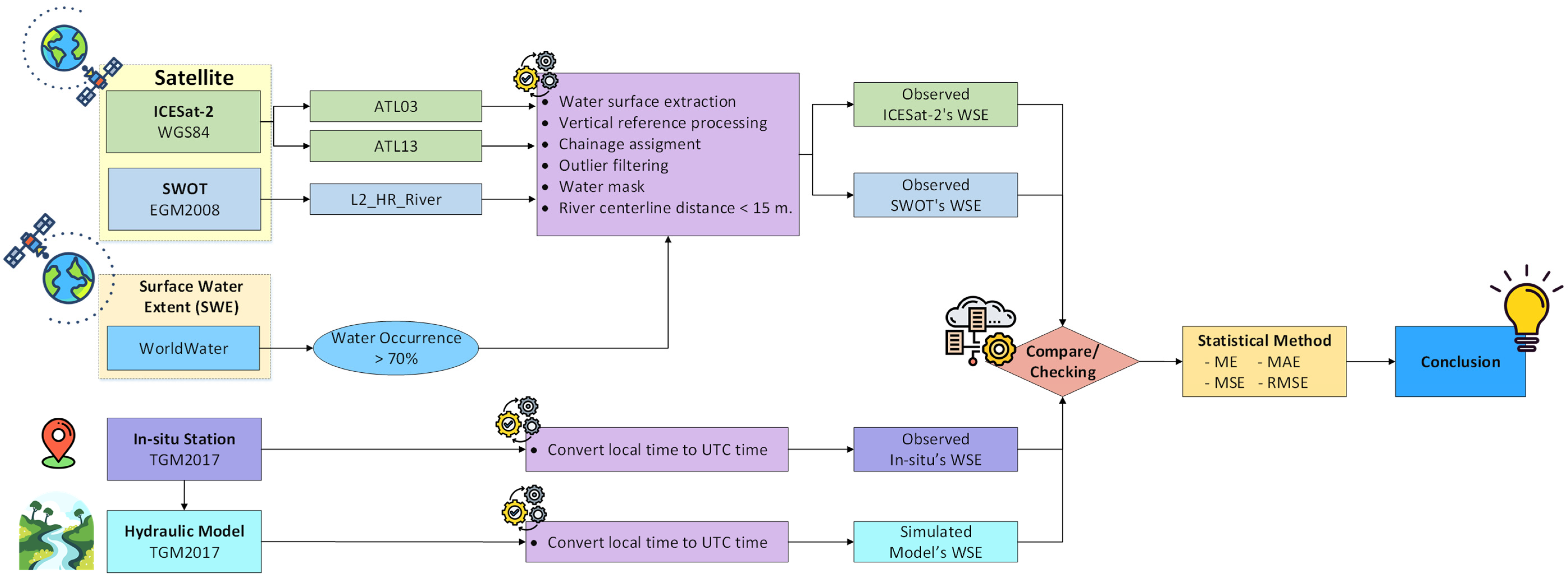
3.5. Water Surface Elevation (WSE) Evaluation
4. Results
4.1. Hydraulic Model Calibration Results
4.2. ICESat-2 ATL03 Data Processing Results
4.3. SWOT Data Processing Results
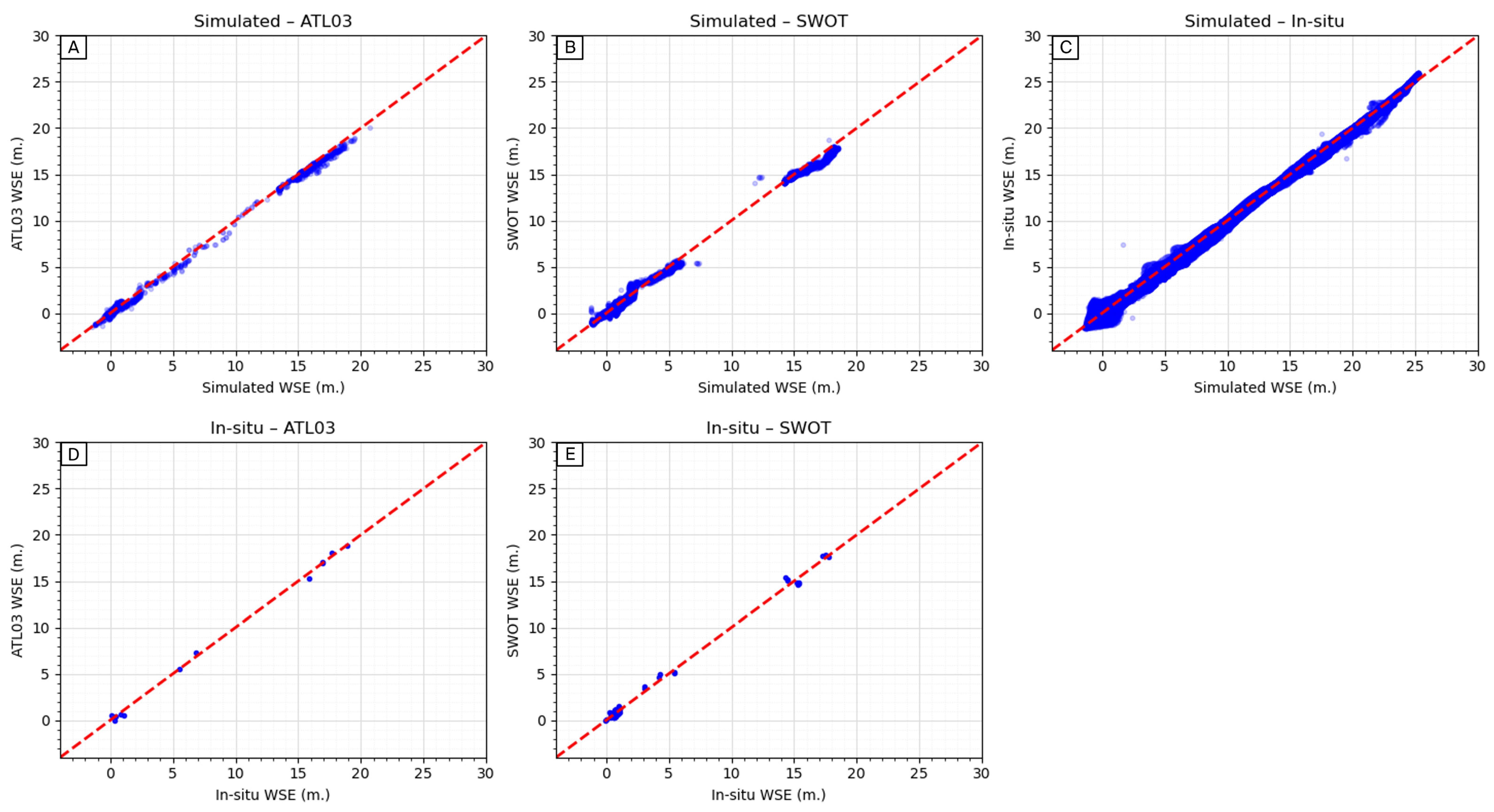
4.4. Evaluation of Water Surface Elevation (WSE) Data Products
5. Discussion
5.1. ICESat-2 Data Selection
5.2. SWOT Data Selection
- (1)
- The L2_HR_LakeSP product provides WSE, area, and storage change data for monitoring lakes and reservoirs.
- (2)
- (3)
- The L2_HR_FPDEM product provides a floodplain digital elevation map in raster format, which can be used to monitor and compare simulated flood maps from flood modeling in terms of depth and area such as [52].
5.3. Model Performance
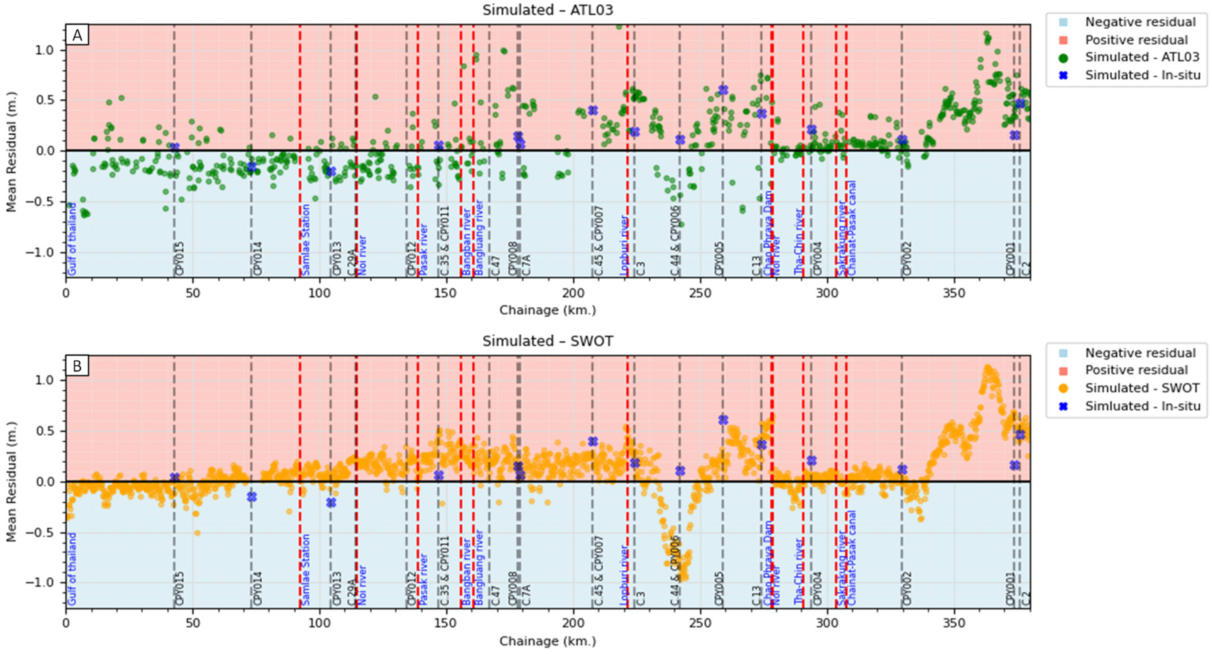
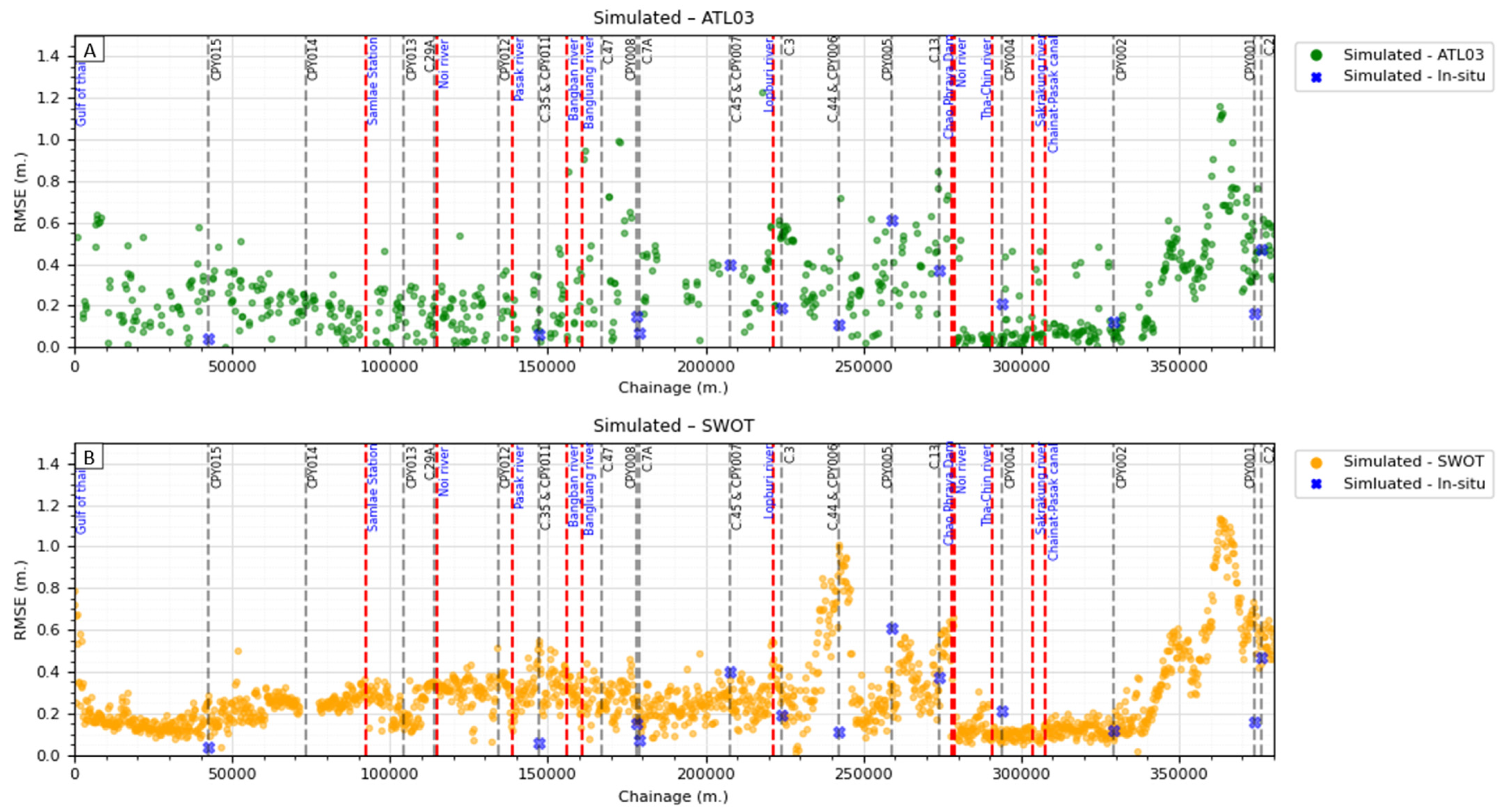
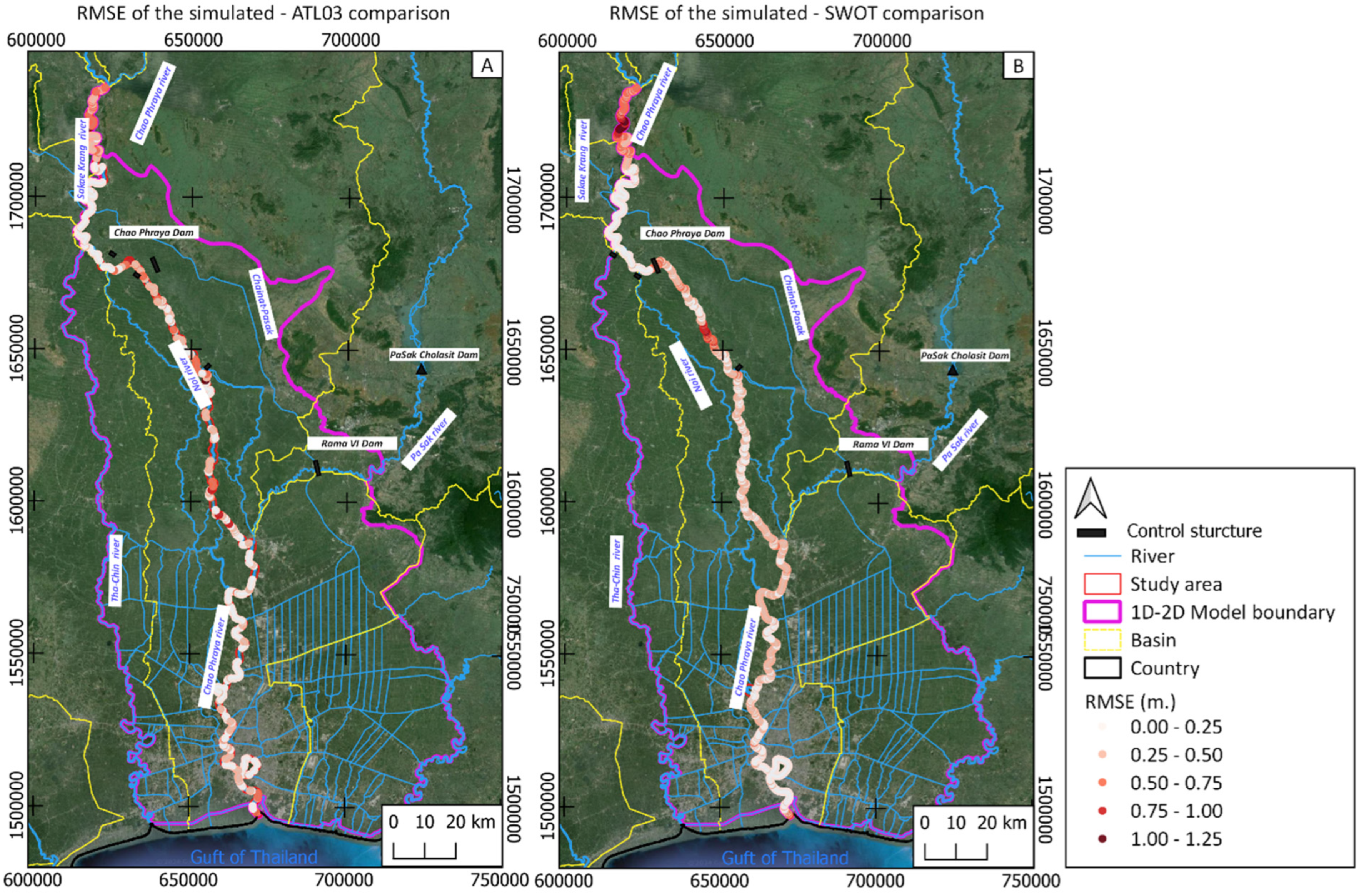
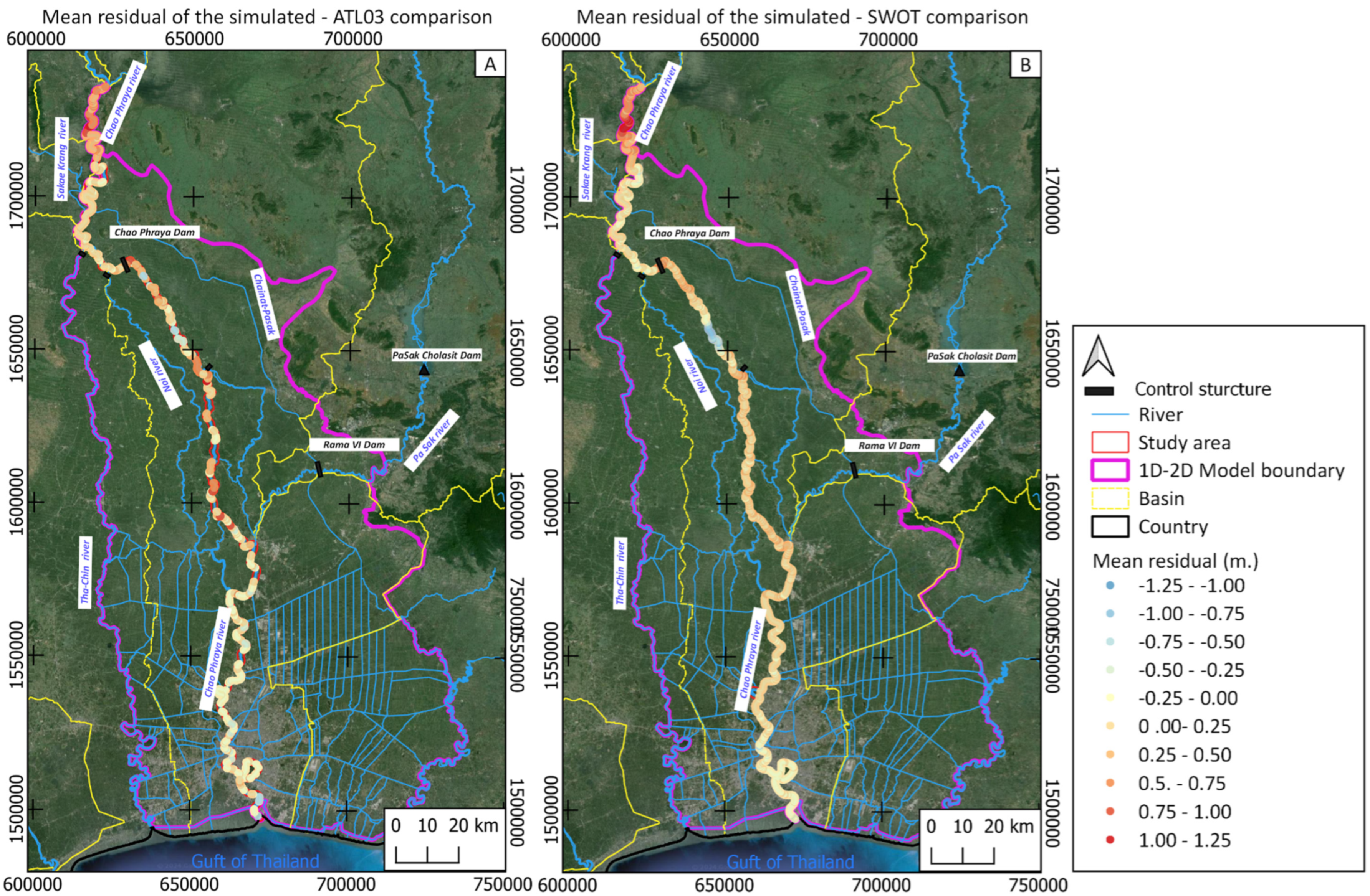
- ▪ Cross-section survey data: The hydraulic model incorporated cross-section survey data collected between 2009 and 2013 for the CPY river. The use of this older data affects the representation of the cross-sectional area and river width as inputs to the hydraulic model, leading to errors in the simulated WSE, particularly in the delta areas. Notably, between chainages 380 km and 330 km, the bottom level of the CPY cross-section profile is higher than that of the adjacent bottom level, resulting in simulated WSE values that are higher than both ATL03 WSE and SWOT WSE, with a mean residual of +1.2 m. Conversely, between chainages 250 km and 230 km, the bottom level is lower than that of the adjacent bottom level, leading to simulated WSE values that are lower than both ATL03 WSE and SWOT WSE, with a mean residual of −0.5 m, as shown in Figure 10. Similar challenges have been observed in studies of the Niger Delta [60], Pacific Ocean, and Japan sea [61] and are relevant to our study area.
- ▪ Water management data: Thailand has many agencies relevant to water management, such as RID, HII, and NAVY, as explained in Section 2.6. Additionally, other water agencies, such as the Metropolitan Waterworks Authority (MWA) provide clean and safe water for public consumption; the Provincial Waterworks Authority (PWA) sources and procures raw water for use in the water supply; and the Department of Drainage and Sewerage (DDS) of the Bangkok Metropolitan Administration (BMA) manages drainage and flood control in Bangkok city. Furthermore, approximately 80 percent of the study area is fully irrigated. These activities impact the flow in the CPY river through pumping operations, but these data were not included in the hydraulic model due to a lack of available data, leading to decreased performance of the simulated WSE. As described by [62], the exclusion of these data led to discharge losses of around 52% from the CPY river. Notably, at a chainage of 96.8 km, the Samlae station operated by MWA pumps approximately 40–50 m³/s to supply drinking water, which was not included in the model.
- ▪ Water management plan data: There are ongoing implementations of water management plans in the study area, such as the Ayutthaya Bypass channel [63] at an upstream chainage of 156.6 km and a downstream chainage of 120 km, along with ongoing land use changes in the lower CPY basin [64], which impact WSE simulations.
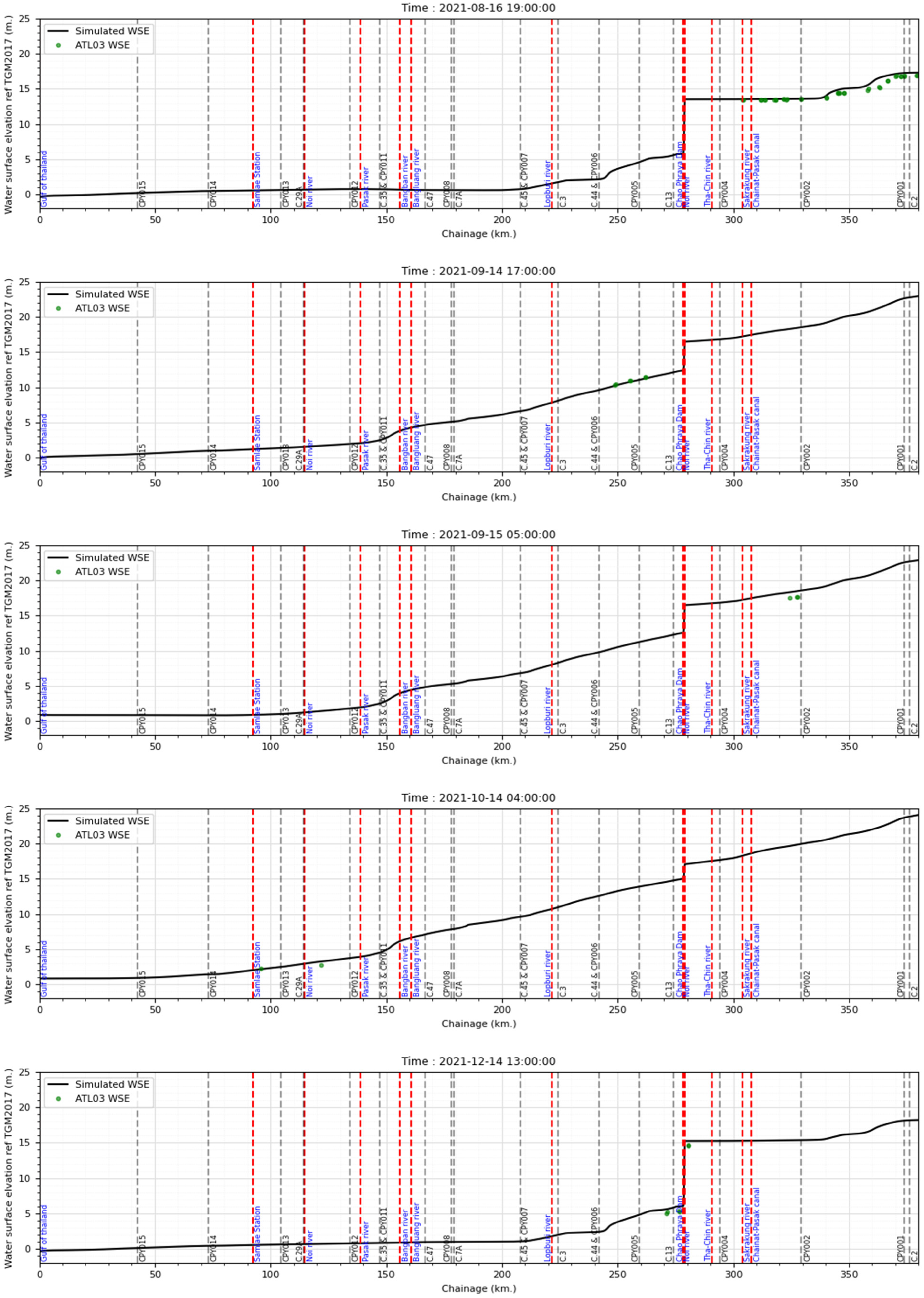
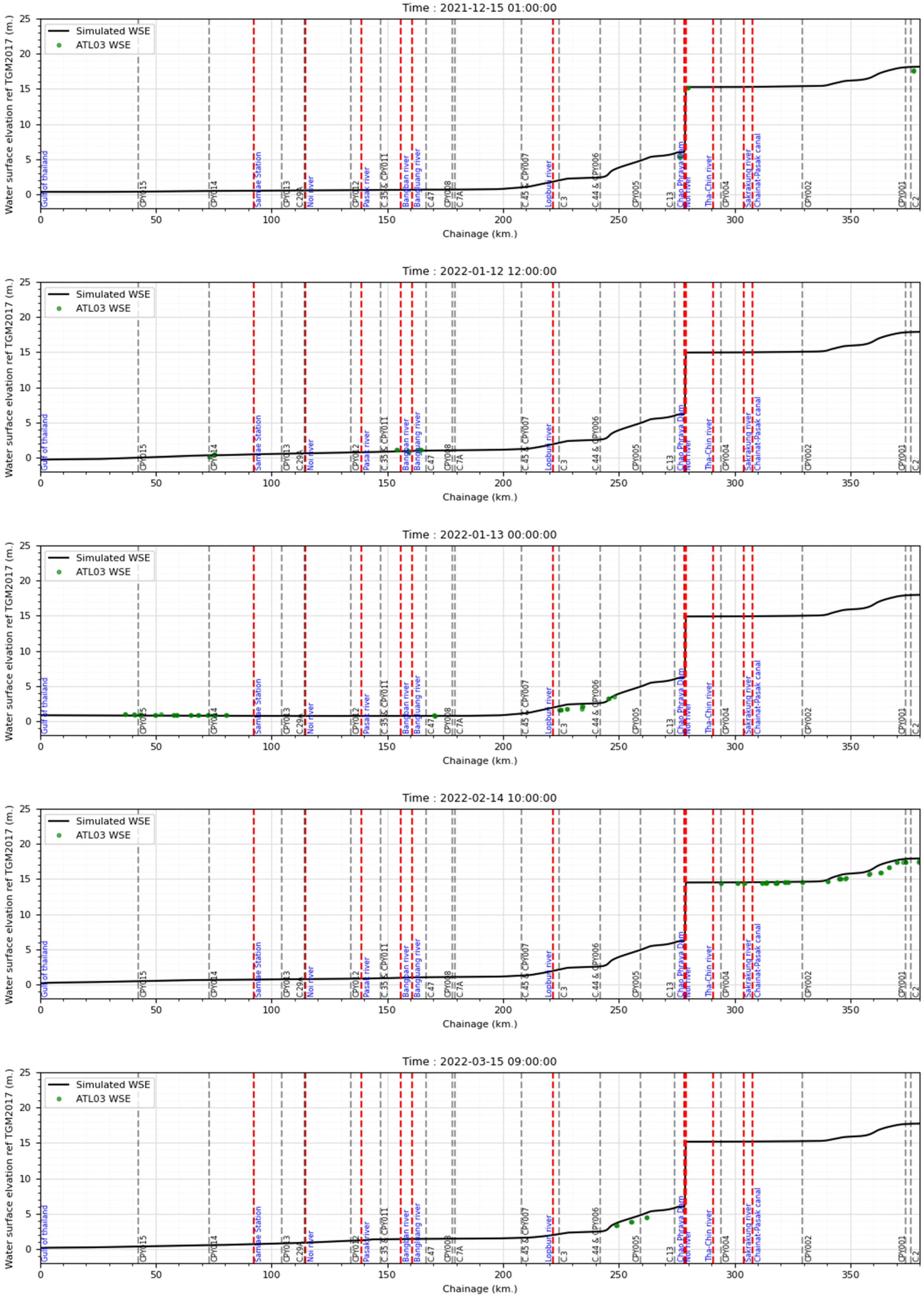
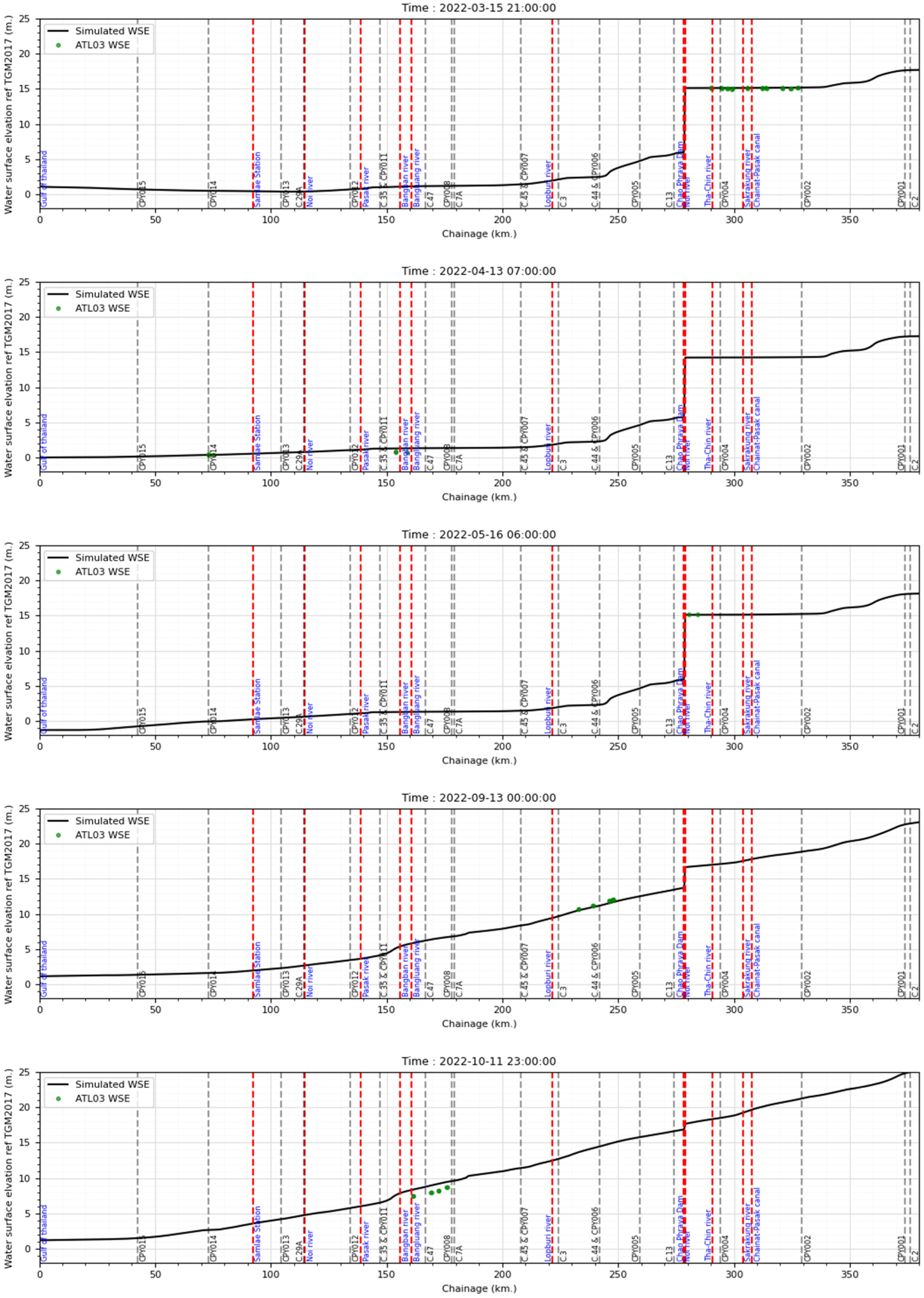
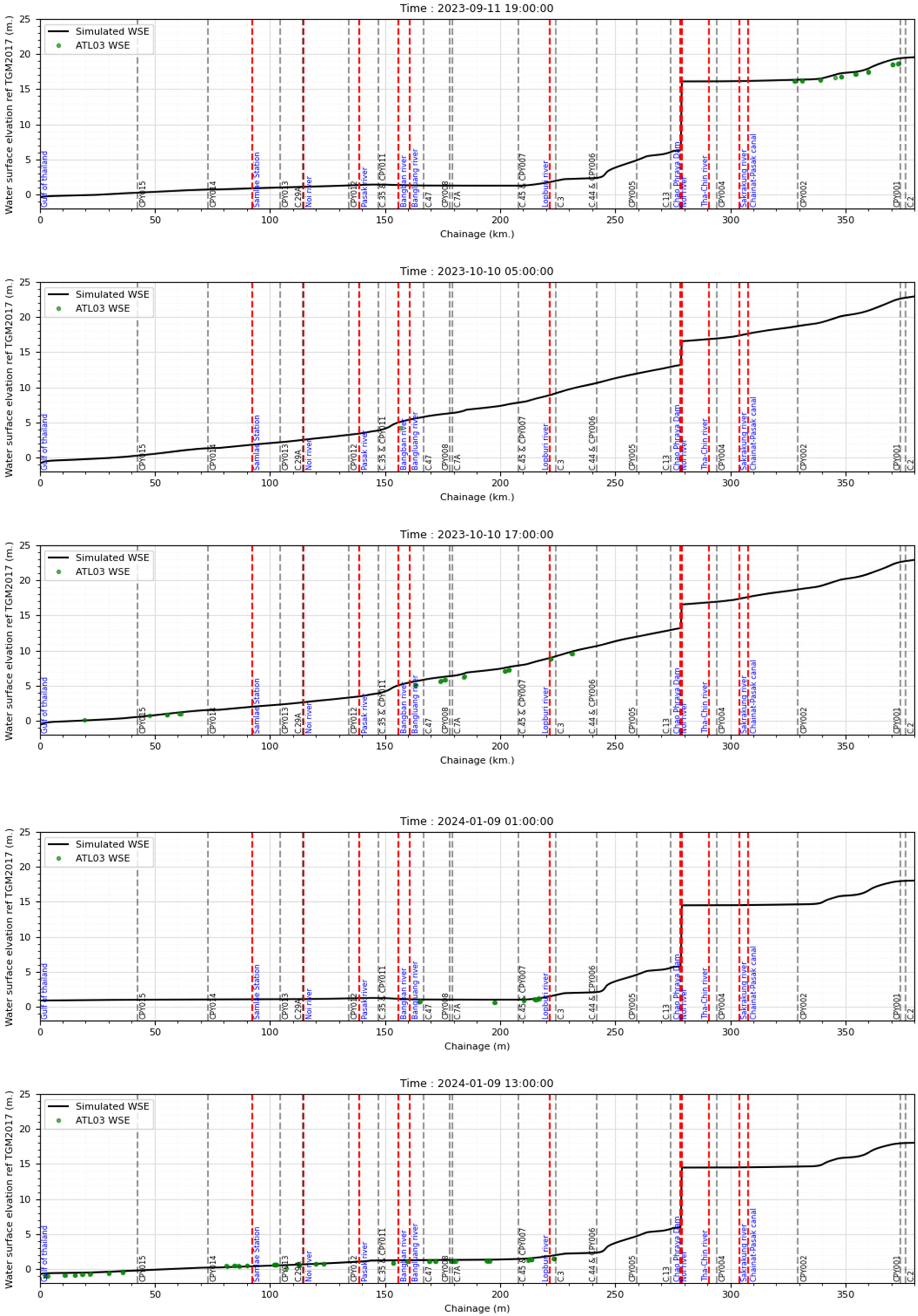
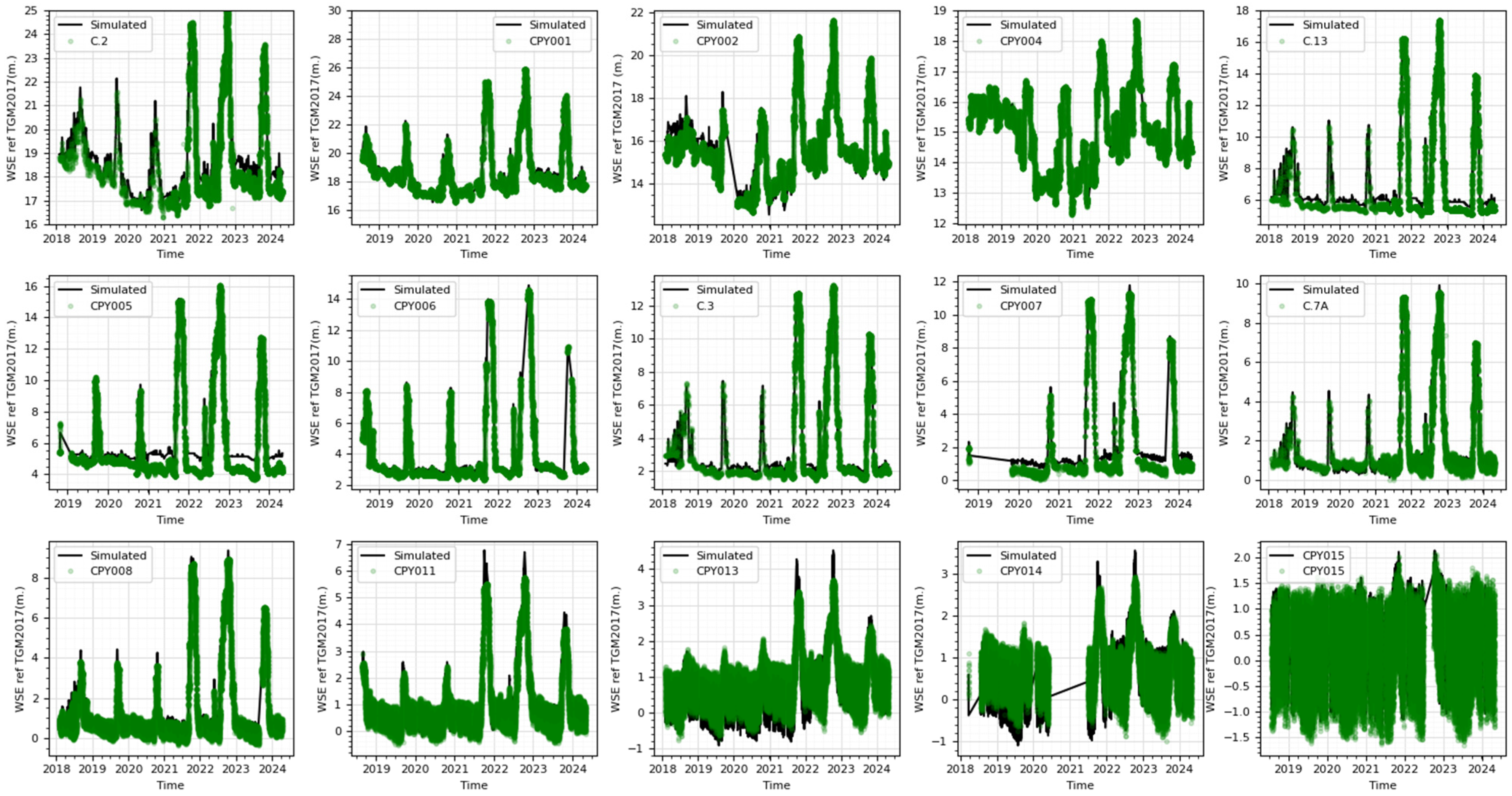
- ▪ Hydraulic model: The process of river hydraulic modeling integrates both hydrological and hydraulic data to simulate river flow and water levels. The performance of the hydraulic model is affected by various factors, such as input data, parameters, control structures, and hydraulic geometry [65]. Additionally, the simulated runoff from the hydrological model contributes to this uncertainty. Meanwhile, the main objectives of the hydraulic model from the operational flood forecasting system are flood warning and flood prediction. The hydraulic model primarily focuses on high-flow conditions. As shown in Figure A3, the simulated WSE performs well under high-flow conditions, whereas it overestimates in situ data under low-flow conditions.
5.4. Model Improvement
- ▪ Cross-section survey: Cross-section data serve as the primary input for the hydraulic model, which simulates cross-sectional area and water level. Updating cross-section data is necessary to keep it current, especially between chainages 380 km and 330 km, and downstream of the CPY dam, from chainage 270 km to 220 km. However, collecting survey data is costly and time-consuming. Estimating the effective cross-section shape using satellite earth observation [48,66] is a viable alternative to reduce the cost and time required for updates.
- ▪ Water management and water management plan data: Collaboration between water management agencies to share data, along with the installation of real-time telemetry, is essential for developing more robust models.
- ▪ Resistance coefficients: Manning’s roughness coefficient [67] is used in the hydraulic model to estimate the mean velocity and discharge in open channels, representing the resistance to flow in channels and floodplains. Adjusting this coefficient can significantly enhance model accuracy, for example by using seasonal variations in Manning’s roughness coefficient [68] or by integrating satellite data (SWOT) to improve roughness estimates along the river [69].
- ▪ Integrating comprehensive data sources: To further enhance model accuracy and reliability, it is crucial to combine various data sources. Integrating in situ data, ATL03 WSE, and SWOT WSE from this study will provide a more comprehensive dataset, allowing for a more robust calibration and validation process and ultimately improving the hydraulic model’s performance.
6. Conclusions
Author Contributions
Funding
Data Availability Statement
Acknowledgments
Conflicts of Interest
Appendix A. ICESat-2 ATL03 Data Processing
Appendix A.1. Illustrates the ICESat-2 ATL03 Data Processing for Each Chainage on 21 November 2018


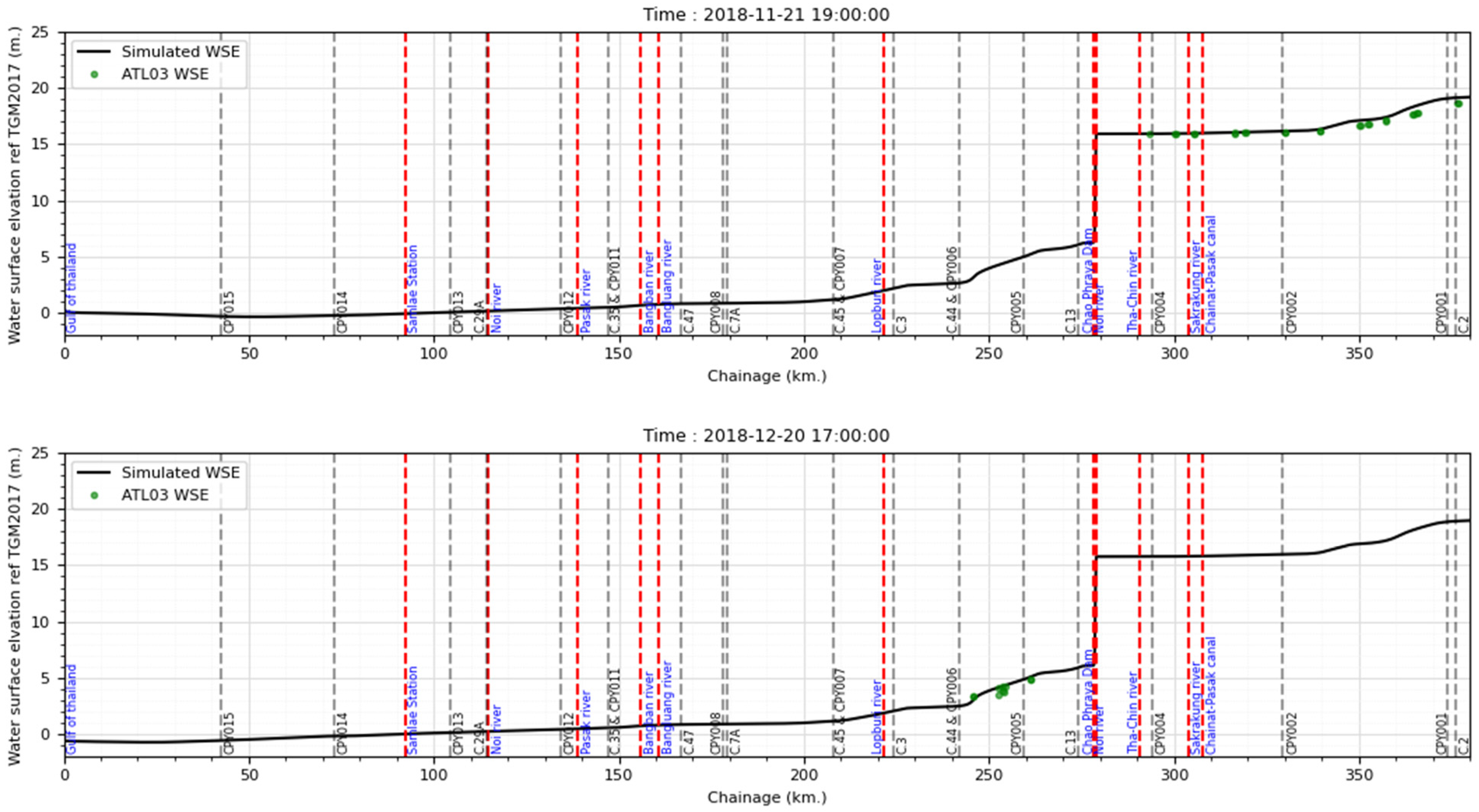
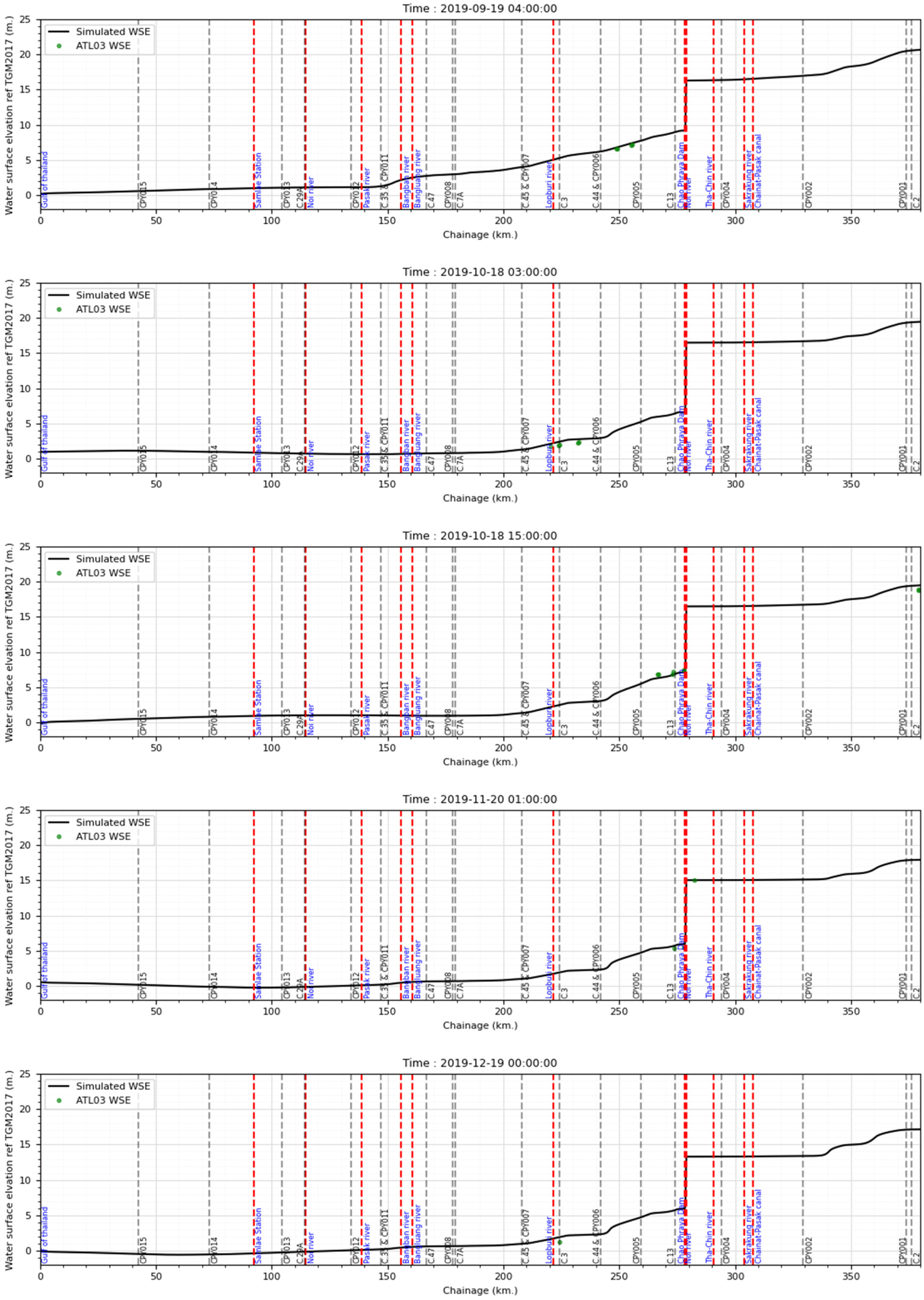
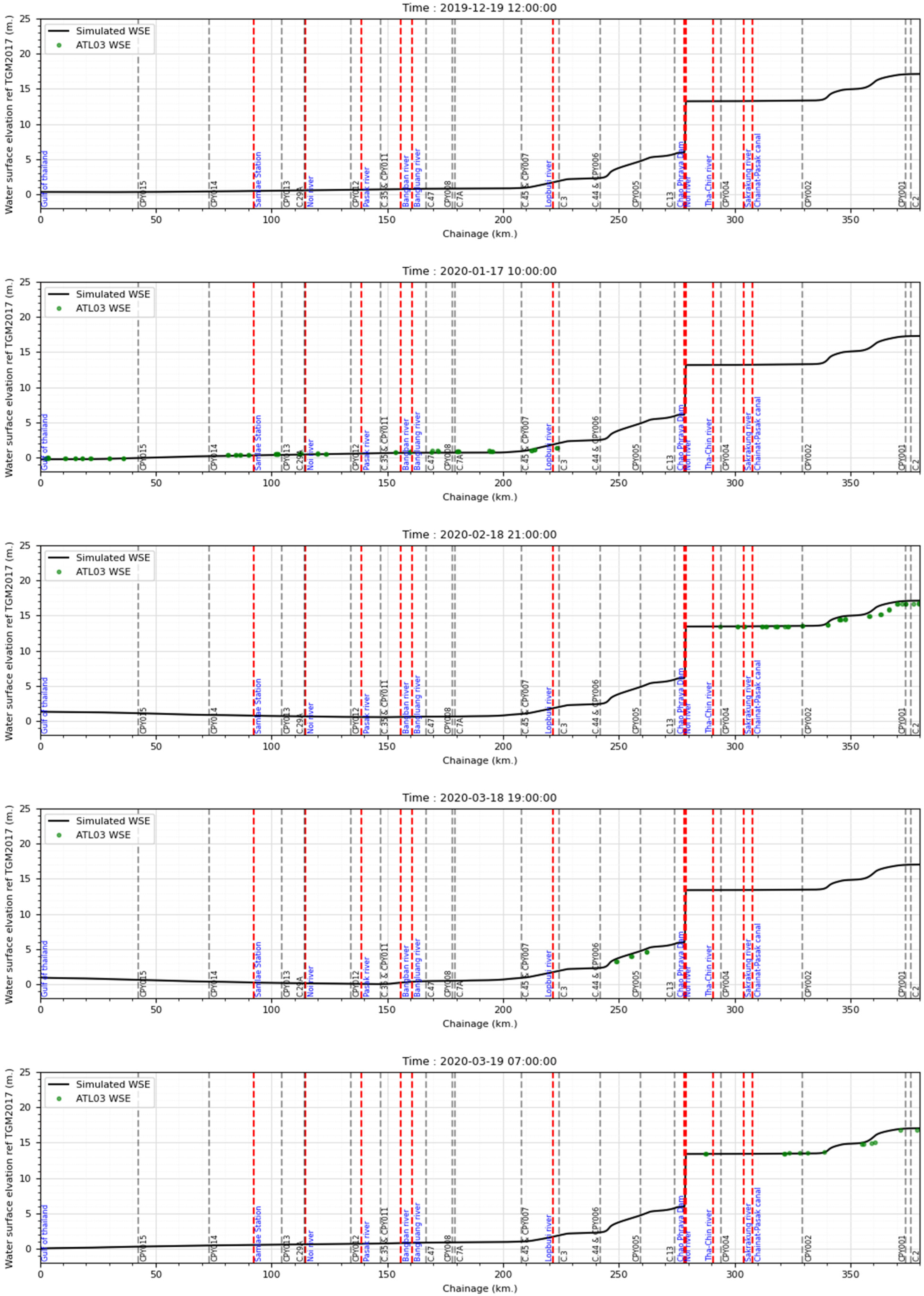
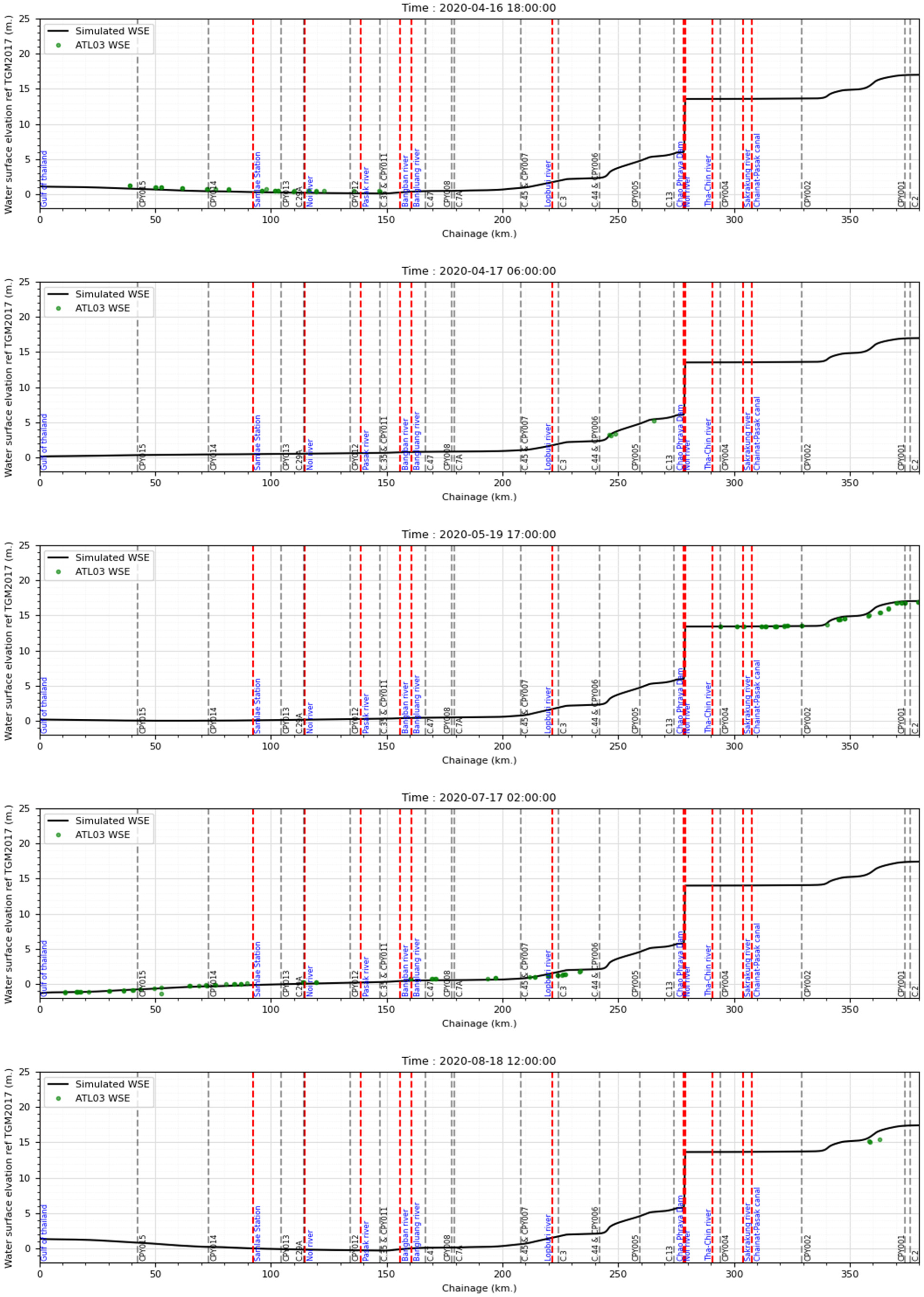
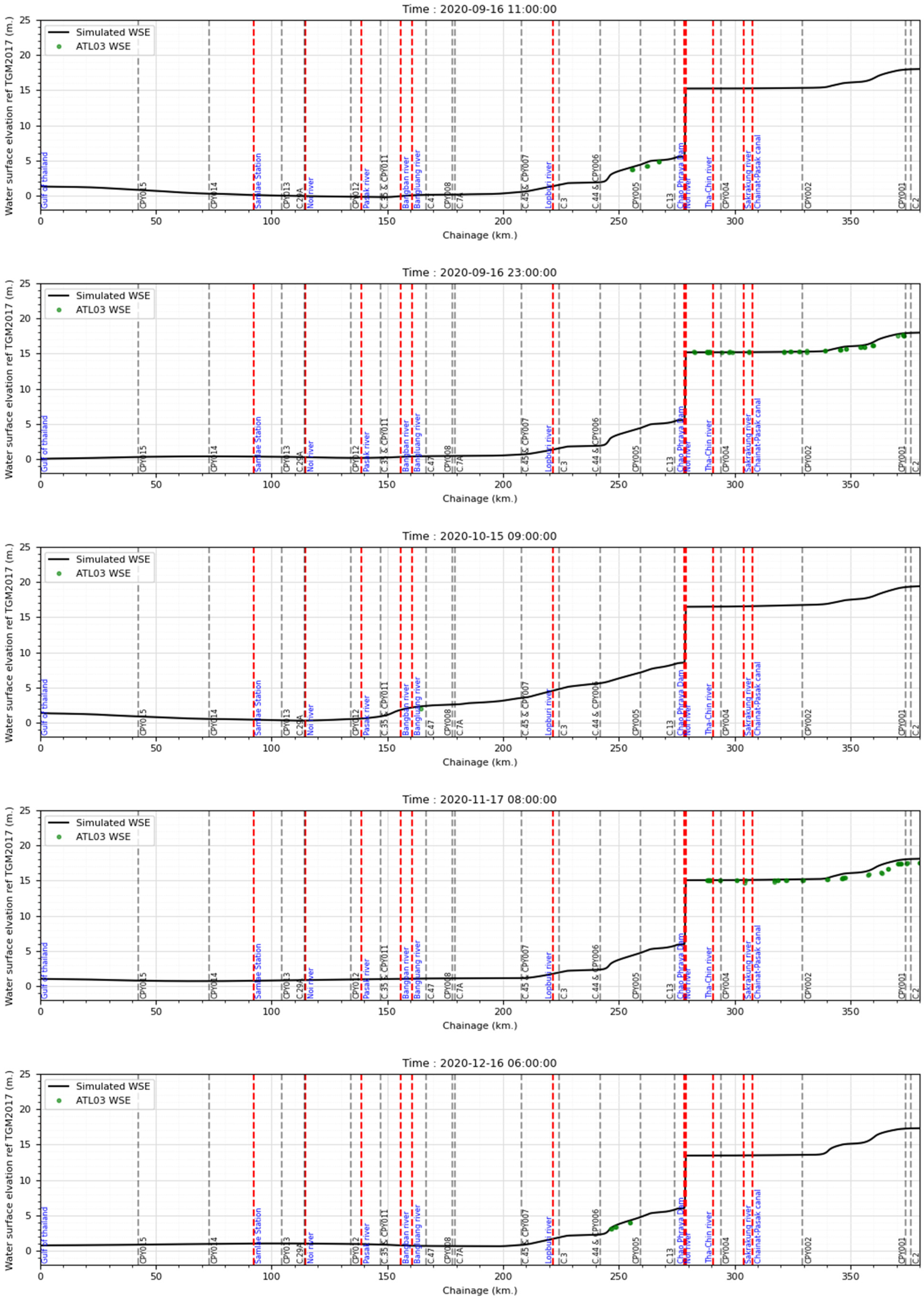
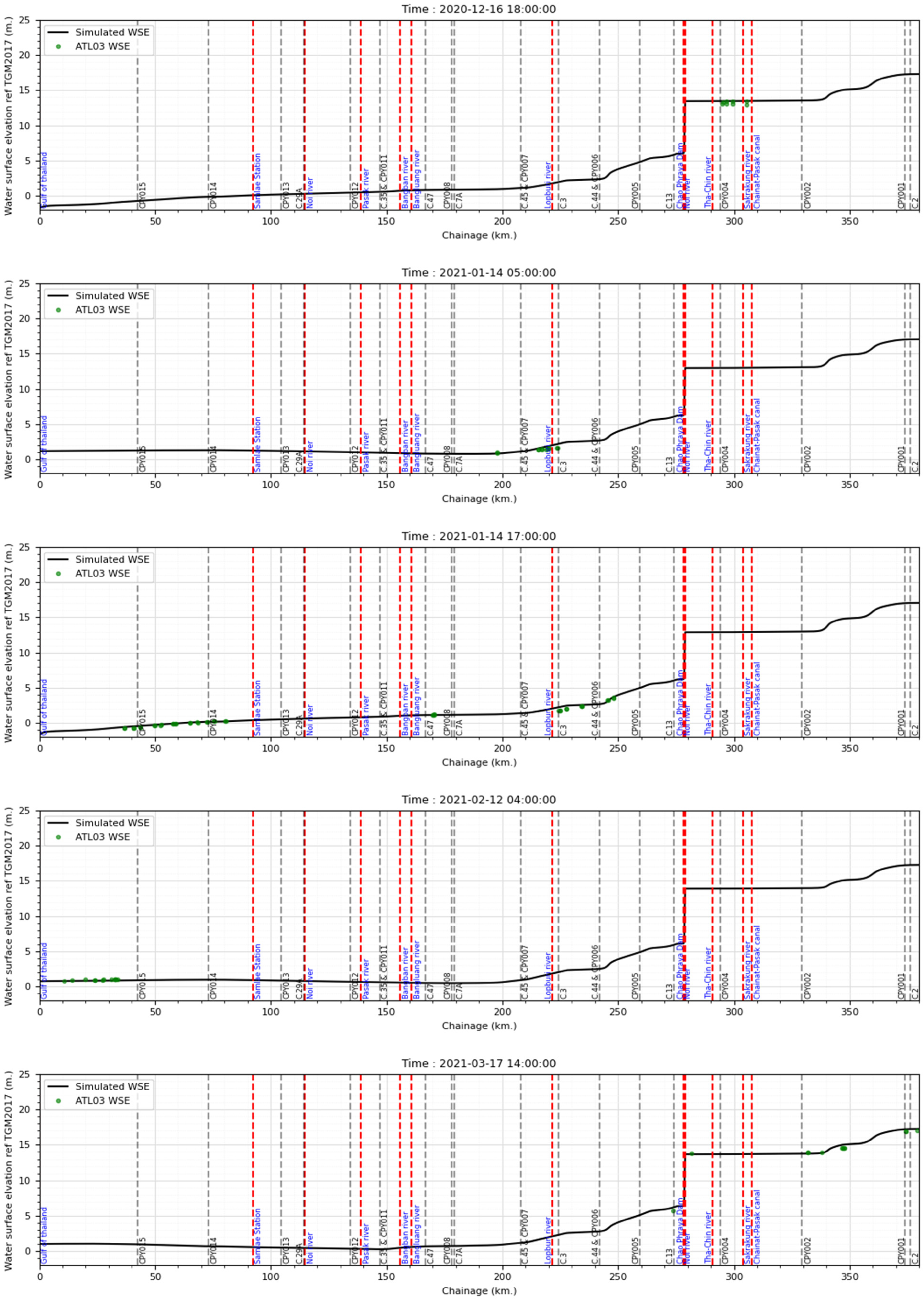
Appendix A.2. Illustrates the Comparison Between Simulated WSE Derived from the Hydraulic Model and ATL03 WSE from ICESat-2 at Various Time Intervals


Appendix B. SWOT Data Processing
Illustrates the Comparison Between Simulated WSE Derived from the Hydraulic Model and SWOT WSE from the SWOT Satellite at Various Time Intervals


Appendix C. Water Surface Elevation (WSE) Evaluation
Appendix C.1. Simulated—In Situ WSE Comparison

Appendix C.2. WSE Profile Comparison
References
- Gasmelseid, T.M. Handbook of Research on Hydroinformatics: Technologies, Theories and Applications; IGI Global: Hershey, PA, USA, 2010; pp. 1–587. [Google Scholar] [CrossRef]
- Wang, L.; Lian, Y.; Li, Z. Hydraulic Analysis for Strategic Management of Flood Risks along the Illinois River. Environ. Earth Sci. 2019, 78, 80. [Google Scholar] [CrossRef]
- Godyn, I. A Revised Approach to Flood Damage Estimation in Flood Risk. Water 2021, 13, 2713. [Google Scholar] [CrossRef]
- Icyimpaye, G.; Abdelbaki, C.; Mourad, K.A. Hydrological and Hydraulic Model for Flood Forecasting in Rwanda. Model. Earth Syst. Environ. 2022, 8, 1179–1189. [Google Scholar] [CrossRef]
- Arduino, G.; Reggiani, P.; Todini, E. Recent Advances in Flood Forecasting and Flood Risk Assessment. Hydrol. Earth Syst. Sci. 2005, 9, 280–284. [Google Scholar] [CrossRef]
- Charoensuk, T.; Lolupiman, T.; Chantip, S.; Sisomphon, P. Modeling Dike Breaching in The Chao Phraya River Basin Using High Resolution Elevation Data (Lidar). In Proceedings of the 13th International Conference on Hydroscience & Engineering. Advancement of Hydro-Engineering for Sustainable Development, Chongqing, China, 18–22 June 2018. [Google Scholar]
- Gu, X.W.; Yang, W.L.; Dong, G.T.; Dang, S.Z. Application of One-Dimensional Hydraulic Model for Flood Simulation in Yellow River Delta. Adv. Mater. Res. 2014, 955–959, 2969–2972. [Google Scholar] [CrossRef]
- Kidson, R.L.; Richards, K.S.; Carling, P.A. Hydraulic Model Calibration for Extreme Floods in Bedrock-Confined Channels: Case Study from Northern Thailand. Hydrol. Process. 2006, 20, 329–344. [Google Scholar] [CrossRef]
- Domeneghetti, A.; Tarpanelli, A.; Brocca, L.; Barbetta, S.; Moramarco, T.; Castellarin, A.; Brath, A. The Use of Remote Sensing-Derived Water Surface Data for Hydraulic Model Calibration. Remote Sens. Environ. 2014, 149, 130–141. [Google Scholar] [CrossRef]
- Lollino, G.; Arattano, M.; Rinaldi, M.; Giustolisi, O.; Marechal, J.C.; Grant, G.E. Engineering Geology for Society and Territory—Volume 3: River Basins, Reservoir Sedimentation and Water Resources; Springer: Berlin/Heidelberg, Germany, 2015; Volume 3, pp. 1–657. [Google Scholar] [CrossRef]
- Kittel, C.M.M.; Hatchard, S.; Neal, J.C.; Nielsen, K.; Bates, P.D.; Bauer-Gottwein, P. Hydraulic Model Calibration Using CryoSat-2 Observations in the Zambezi Catchment. Water Resour. Res. 2021, 57, e2020WR029261. [Google Scholar] [CrossRef]
- Domeneghetti, A.; Molari, G.; Tourian, M.J.; Tarpanelli, A.; Behnia, S.; Moramarco, T.; Sneeuw, N.; Brath, A. Testing the Use of Single- and Multi-Mission Satellite Altimetry for the Calibration of Hydraulic Models. Adv. Water Resour. 2021, 151, 103887. [Google Scholar] [CrossRef]
- Neumann, T.A.; Martino, A.J.; Markus, T.; Bae, S.; Bock, M.R.; Brenner, A.C.; Brunt, K.M.; Cavanaugh, J.; Fernandes, S.T.; Hancock, D.W.; et al. The Ice, Cloud, and Land Elevation Satellite—2 Mission: A Global Geolocated Photon Product Derived from the Aadvanced Ttopographic Llaser Aaltimeter Ssystem. Remote Sens. Environ. 2019, 233, 111325. [Google Scholar] [CrossRef] [PubMed]
- Dandabathula, G.; Srinivasa Rao, S. Validation of ICESat-2 Surface Water Level Product ATL13 with Near Real Time Gauge Data. Hydrology 2020, 8, 19. [Google Scholar] [CrossRef]
- Yuan, C.; Gong, P.; Bai, Y. Performance Assessment of ICESat-2 Laser Altimeter Data for Water-Level Measurement over Lakes and Reservoirs in China. Remote Sensing 2020, 12, 770. [Google Scholar] [CrossRef]
- Guo, X.; Jin, S.; Zhang, Z. Evaluation of Water Level Estimation in the Upper Yangtze River from ICESat-2 Data. Prog. Electromagn. Res. Symp. 2021, 2021, 2260–2264. [Google Scholar] [CrossRef]
- Xie, J.; Li, B.; Jiao, H.; Zhou, Q.; Mei, Y.; Xie, D.; Wu, Y.; Sun, X.; Fu, Y. Water Level Change Monitoring Based on a New Denoising Algorithm Using Data from Landsat and ICESat-2: A Case Study of Miyun Reservoir in Beijing. Remote Sensing 2022, 14, 4344. [Google Scholar] [CrossRef]
- Zhou, H.; Liu, S.; Mo, X.; Hu, S.; Zhang, L.; Ma, J.; Bandini, F.; Grosen, H.; Bauer-Gottwein, P. Calibrating a Hydrodynamic Model Using Water Surface Elevation Determined from ICESat-2 Derived Cross-Section and Sentinel-2 Retrieved Sub-Pixel River Width. Remote Sens. Environ. 2023, 298, 113796. [Google Scholar] [CrossRef]
- Scherer, D.; Schwatke, C.; Dettmering, D.; Seitz, F. ICESat-2 Based River Surface Slope and Its Impact on Water Level Time Series From Satellite Altimetry. Water Resour. Res. 2022, 58, e2022WR032842. [Google Scholar] [CrossRef]
- Narin, O.G.; Abdikan, S. Multi-Temporal Analysis of Inland Water Level Change Using ICESat-2 ATL-13 Data in Lakes and Dams. Environ. Sci. Pollut. Res. 2023, 30, 15364–15376. [Google Scholar] [CrossRef] [PubMed]
- Chen, Y.; Liu, Q.; Ticehurst, C.; Sarker, C.; Karim, F.; Penton, D.; Sengupta, A. Refining ICESAT-2 ATL13 Altimetry Data for Improving Water Surface Elevation Accuracy on Rivers. Remote Sens. 2024, 16, 1706. [Google Scholar] [CrossRef]
- Fjørtoft, R.; Gaudin, J.M.; Pourthié, N.; Lalaurie, J.C.; Mallet, A.; Nouvel, J.F.; Martinot-Lagarde, J.; Oriot, H.; Borderies, P.; Ruiz, C.; et al. KaRIn on SWOT: Characteristics of near-Nadir Ka-Band Interferometric SAR Imagery. IEEE Trans. Geosci. Remote Sens. 2014, 52, 2172–2185. [Google Scholar] [CrossRef]
- Durand, M.; Neal, J.; Rodríguez, E.; Andreadis, K.M.; Smith, L.C.; Yoon, Y. Estimating Reach-Averaged Discharge for the River Severn from Measurements of River Water Surface Elevation and Slope. J. Hydrol. 2014, 511, 92–104. [Google Scholar] [CrossRef]
- Cha, Y.; Park, S.S.; Kim, K.; Byeon, M.; Stow, C.A. Reply to comment by J. S. Selker et al. on “Capabilities and limitations of tracing spatial temperature patterns by fiber-optic distributed temperature sensing”. Water Resour. Res. 2014, 50, 5375–5377. [Google Scholar] [CrossRef]
- Langhorst, T.; Pavelsky, T.M.; Frasson, R.P.d.M.; Wei, R.; Domeneghetti, A.; Altenau, E.H.; Durand, M.T.; Minear, J.T.; Wegmann, K.W.; Fuller, M.R. Anticipated Improvements to River Surface Elevation Profiles from the Surface Water and Ocean Topography Mission. Front. Earth Sci. 2019, 7, 102. [Google Scholar] [CrossRef]
- Chevalier, L.; Desroches, D.; Laignel, B.; Fjortoft, R.; Turki, I.; Allain, D.; Lyard, F.; Blumstein, D.; Salameh, E. High-Resolution SWOT Simulations of the Macrotidal Seine Estuary in Different Hydrodynamic Conditions. IEEE Geosci. Remote Sens. Lett. 2019, 16, 5–9. [Google Scholar] [CrossRef]
- Sisomphon, P.; Boonya-aroonnet, S.; Chonwattana, S. Towards the development of a decision support system for flood management in chao phraya river basin, thailand. In Proceedings of the International Conference on Flood Resilience, Experiences in Asia and Europe, Exeter, UK, 5–7 September 2013. [Google Scholar]
- Charoensuk, T.; Luchner, J.; Balbarini, N.; Sisomphon, P.; Bauer-Gottwein, P. Enhancing the Capabilities of the Chao Phraya Forecasting System through the Integration of Pre-Processed Numerical Weather Forecasts. J. Hydrol. Reg. Stud. 2024, 52, 101737. [Google Scholar] [CrossRef]
- DHI Water and Environment. MIKE 11 Reference Manual; Scribd: San Francisco, CA, USA, 2021; ISBN 1672-1683. [Google Scholar]
- DHI MIKE 21 FLOW MODEL FM, Reference Mannual; Scribd: San Francisco, CA, USA, 2018; Volume 55.
- DHI Water and Environment. MIKE FLOOD Reference Manual; Scribd: San Francisco, CA, USA, 2019; Volume 37. [Google Scholar]
- Markus, T.; Neumann, T.; Martino, A.; Abdalati, W.; Brunt, K.; Csatho, B.; Farrell, S.; Fricker, H.; Gardner, A.; Harding, D.; et al. The Ice, Cloud, and Land Elevation Satellite-2 (ICESat-2): Science Requirements, Concept, and Implementation. Remote Sens. Environ. 2017, 190, 260–273. [Google Scholar] [CrossRef]
- Tom Neumann; Anita Brenner; David Hancock; John Robbins; Jack Saba; Kaitlin Harbeck; Aimée Gibbons; Jeffrey Lee; Scott Luthcke; Tim Rebold Algorithm Theoretical Basis Document (ATBD) for Global Geolocated Photons ATL03. Remote Sens. Environ. 2021, 2, 7–208.
- Jasinski, M.; Gsfc, N.; Stoll, J.; Hancock, D.; Robbins, J.; Nattala, J.; Morison, J.; Jones, B.; Ondrusek, M.; Parrish, C.; et al. ICESat-2 Algorithm Theoretical Basis Document (ATBD) for Along Track Inland Surface Water Data, ATL13, Version 6; Goddard Space Flight Center Greenbelt, NASA: Greenbelt, MD, USA, 2023; Volume 2. [CrossRef]
- Biancamaria, S.; Lettenmaier, D.P.; Pavelsky, T.M. The SWOT Mission and Its Capabilities for Land Hydrology. Surv. Geophys. 2016, 37, 307–337. [Google Scholar] [CrossRef]
- Desai, S.; Chen, C.; Picot, N.; Fjørtoft, R.; Bohe, A. SWOT Project Release Note for Sample Data Products; NASA: Greenbelt, MD, USA, 2021; Volume 16.
- Surface Water Ocean Topography (SWOT). 2024. SWOT Level 2 River Single-Pass Vector Data Product, Version C. Ver. C. PO.DAAC, CA, USA. Dataset. Available online: https://doi.org/10.5067/SWOT-RIVERSP-2.0 (accessed on 5 May 2024).
- JPLD-56413 Revision B. SWOT Product Description Document: Level 2 KaRIn High Rate River Single Pass Vector (L2_HR_RiverSP) Data Product. In Jet Propulsion Laboratory Internal Document; NASA SWOT: Hawthorne, CA, USA, 2023.
- Tottrup, C.; Druce, D.; Meyer, R.P.; Christensen, M.; Riffler, M.; Dulleck, B.; Rastner, P.; Jupova, K.; Sokoup, T.; Haag, A.; et al. Surface Water Dynamics from Space: A Round Robin Intercomparison of Using Optical and SAR High-Resolution Satellite Observations for Regional Surface Water Detection. Remote Sens. 2022, 14, 2410. [Google Scholar] [CrossRef]
- Dumrongchai, P.; Srimanee, C.; Duangdee, N.; Bairaksa, J. The Determination of Thailand Geoid Model 2017 (TGM2017) from Airborne and Terrestrial Gravimetry. Terr. Atmos. Ocean. Sci. 2021, 32, 859–874. [Google Scholar] [CrossRef]
- Lian, W.; Zhang, G.; Cui, H.; Chen, Z.; Wei, S.; Zhu, C.; Xie, Z. Extraction of High-Accuracy Control Points Using ICESat-2 ATL03 in Urban Areas. Int. J. Appl. Earth Obs. Geoinf. 2022, 115, 103116. [Google Scholar] [CrossRef]
- Smith, B.; Fricker, H.A.; Holschuh, N.; Gardner, A.S.; Adusumilli, S.; Brunt, K.M.; Csatho, B.; Harbeck, K.; Huth, A.; Neumann, T.; et al. Land Ice Height-Retrieval Algorithm for NASA’s ICESat-2 Photon-Counting Laser Altimeter. Remote Sens. Environ. 2019, 233, 111352. [Google Scholar] [CrossRef]
- Pearson, R.K.; Neuvo, Y.; Astola, J.; Gabbouj, M. Generalized Hampel Filters. Eurasip J. Adv. Signal Process. 2016, 2016, 87. [Google Scholar] [CrossRef]
- Coppo Frias, M.; Liu, S.; Mo, X.; Nielsen, K.; Ranndal, H.; Jiang, L.; Ma, J.; Bauer-Gottwein, P. River Hydraulic Modeling with ICESat-2 Land and Water Surface Elevation. Hydrol. Earth Syst. Sci. 2023, 27, 1011–1032. [Google Scholar] [CrossRef]
- Pavlis, N.K.; Holmes, S.A.; Kenyon, S.C.; Factor, J.K. The Development and Evaluation of the Earth Gravitational Model 2008 (EGM2008). J. Geophys. Res. Solid Earth 2012, 117, 1–12. [Google Scholar] [CrossRef]
- Cleveland, W.S. Robust Locally Weighted Regression and Smoothing Scatterplots. J. Am. Stat. Assoc. 1979, 74, 829–836. [Google Scholar] [CrossRef]
- Xu, N.; Zheng, H.; Ma, Y.; Yang, J.; Liu, X.; Wang, X. Global Estimation and Assessment of Monthly Lake/Reservoir Water Level Changes Using ICESat-2 ATL13 Products. Remote Sens. 2021, 13, 2744. [Google Scholar] [CrossRef]
- Musaeus, A.F.; Kittel, C.M.M.; Luchner, J.; Frias, M.C.; Bauer-Gottwein, P. Hydraulic River Models From ICESat-2 Elevation and Water Surface Slope. Water Resour. Res. 2024, 60, e2023WR036428. [Google Scholar] [CrossRef]
- Yamazaki, D.; Ikeshima, D.; Tawatari, R.; Yamaguchi, T.; O’Loughlin, F.; Neal, J.C.; Sampson, C.C.; Kanae, S.; Bates, P.D. A High-Accuracy Map of Global Terrain Elevations. Geophys. Res. Lett. 2017, 44, 5844–5853. [Google Scholar] [CrossRef]
- Li, Y.; Gao, H.; Jasinski, M.F.; Zhang, S.; Stoll, J.D. Deriving High-Resolution Reservoir Bathymetry from ICESat-2 Prototype Photon-Counting Lidar and Landsat Imagery. IEEE Trans. Geosci. Remote Sens. 2019, 57, 7883–7893. [Google Scholar] [CrossRef]
- Bergeron, J.; Siles, G.; Leconte, R.; Trudel, M.; Desroches, D.; Peters, D.L. Assessing the Capabilities of the Surface Water and Ocean Topography (SWOT) Mission for Large Lake Water Surface Elevation Monitoring under Different Wind Conditions. Hydrol. Earth Syst. Sci. 2020, 24, 5985–6000. [Google Scholar] [CrossRef]
- Frasson, R.P.d.M.; Schumann, G.J.P.; Kettner, A.J.; Brakenridge, G.R.; Krajewski, W.F. Will the Surface Water and Ocean Topography (SWOT) Satellite Mission Observe Floods? Geophys. Res. Lett. 2019, 46, 10435–10445. [Google Scholar] [CrossRef]
- Domeneghetti, A.; Schumann, G.J.P.; Frasson, R.P.M.; Wei, R.; Pavelsky, T.M.; Castellarin, A.; Brath, A.; Durand, M.T. Characterizing Water Surface Elevation under Different Flow Conditions for the Upcoming SWOT Mission. J. Hydrol. 2018, 561, 848–861. [Google Scholar] [CrossRef]
- Frasson, R.P.d.M.; Pavelsky, T.M.; Fonstad, M.A.; Durand, M.T.; Allen, G.H.; Schumann, G.; Lion, C.; Beighley, R.E.; Yang, X. Global Relationships Between River Width, Slope, Catchment Area, Meander Wavelength, Sinuosity, and Discharge. Geophys. Res. Lett. 2019, 46, 3252–3262. [Google Scholar] [CrossRef]
- JPL D-105505 “Algorithm Theoretical Basis Document (ATBD) for Level 2 KaRIn High Rate River Single Pass Science Algorithm Software”. In Jet Propulsion Laboratory Internal Document 2023; NASA SWOT: Hawthorne, CA, USA, 2023; pp. 1–54.
- Andreadis, K.M.; Clark, E.A.; Lettenmaier, D.P.; Alsdorf, D.E. Prospects for River Discharge and Depth Estimation through Assimilation of Swath-Altimetry into a Raster-Based Hydrodynamics Model. Geophys. Res. Lett. 2007, 34, 1–5. [Google Scholar] [CrossRef]
- Biancamaria, S.; Durand, M.; Andreadis, K.M.; Bates, P.D.; Boone, A.; Mognard, N.M.; Rodríguez, E.; Alsdorf, D.E.; Lettenmaier, D.P.; Clark, E.A. Assimilation of Virtual Wide Swath Altimetry to Improve Arctic River Modeling. Remote Sens. Environ. 2011, 115, 373–381. [Google Scholar] [CrossRef]
- Munier, S.; Polebistki, A.; Brown, C.; Belaud, G.; Lettenmaier, D.P. SWOT Data Assimilation for Operational Reservoir Management on the Upper Niger River Basin. Water Resour. Res. 2015, 51, 554–575. [Google Scholar] [CrossRef]
- Elmer, N.J.; Hain, C.; Hossain, F.; Desroches, D.; Pottier, C. Generating Proxy SWOT Water Surface Elevations Using WRF-Hydro and the CNES SWOT Hydrology Simulator. Water Resour. Res. 2020, 56, e2020WR027464. [Google Scholar] [CrossRef]
- Abam, T.K.S.; Omuso, W.O. On River Cross-Sectional Change in the Niger Delta. Geomorphology 2000, 34, 111–126. [Google Scholar] [CrossRef]
- Ogawa, Y.; Fujita, Y.; Shuto, N. Change in the Cross-Sectional Area and Topography at River Mouth. Coast. Eng. Jpn. 1984, 27, 233–247. [Google Scholar] [CrossRef]
- Chettanawanit, K.; Charoensuk, T.; Luangdilok, N.; Thanathanphon, W.; Mooktaree, A.; Lolupiman, T.; Kyaw, K.K.; Sisomphon, P. Simulation of Water Losses for the 1D Salinity Forecasting Model in Chao Phraya River. Eng. Access 2022, 8, 161–166. [Google Scholar] [CrossRef]
- JICA. Data Collection Survey on the Outer Ring Road Diversion Channel in the Comprehensive Flood Management Plan for the Chao Phraya River Basin in the Kingdom of Thailand; JICA: Tokyo, Japan, 2018.
- Visessri, S.; Ekkawatpanit, C. Flood Management in the Context of Climate and Land-Use Changes and Adaptation within the Chao Phraya River Basin. J. Disaster Res. 2020, 15, 579–587. [Google Scholar] [CrossRef]
- Mohd Anuar, M.A.; Mohd Adnan, M.S.; Lim, F.H. Uncertainty in River Hydraulic Modelling: A Review for Fundamental Understanding; Springer: Singapore, 2022; Volume 214, ISBN 9789811679193. [Google Scholar]
- Bauer-Gottwein, P.; Zakharova, E.; Coppo Frías, M.; Ranndal, H.; Nielsen, K.; Christoffersen, L.; Liu, J.; Jiang, L. A Hydraulic Model of the Amur River Informed by ICESat-2 Elevation. Hydrol. Sci. J. 2023, 68, 2027–2041. [Google Scholar] [CrossRef]
- Chow, V. Te Applied Hydrology. J. Hydrol. 1968, 6, 224–225. [Google Scholar] [CrossRef]
- Hadiani, M.O.; Gholami, V.; Azar, Z. Investigation on the Effect of the Season in Determination of Manning Roughness Coefficient in Predicting Flood Hydraulic Behavior (Case Study: Haraz River). J. Environ. Stud. 2009, 35, 11–18. [Google Scholar]
- de Moraes Frasson, R.P. Chapter 5—Using the Surface Water and Ocean Topography Mission Data to Estimate River Bathymetry and Channel Roughness. In Earth Observation, Earth Observation for Flood Applications; Elsevier Ltd.: Amsterdam, The Netherlands, 2021; pp. 105–128. ISBN 9780128194126. [Google Scholar]


| Dataset | Data Collection | Repeat Cycle | Datum Reference | |
|---|---|---|---|---|
| Satellite products | ||||
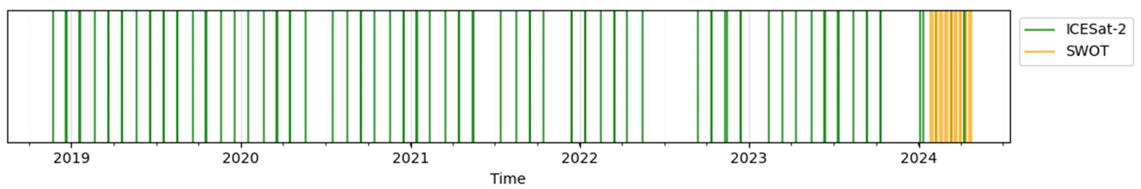
| ICESat-2 ATL03 | Global Geolocated Photon Data | 21 Nov 2018–9 Apr 2024 | 91 days | WGS84 ellipsoid |
| ICESat-2 ATL13 | Inland Water Surface Height | 20 Dec 2018–9 Apr 2024 | 91 days | WGS84 ellipsoid |
| SWOT L2_HR_RiverSP_2.0 | Surface Water and Ocean Topography mission | 26 Jan 2024–22 Apr 2024 | 21 days | EGM2008 geoid |
| WorldWater’s SWE | Water occurrence | 2017–2021 | - | - |
| In situ | ||||
| HII station | WSE | 1 Jan 2018–30 Apr 2024 | Hourly | TGM2017 |
| RID station | Discharge and WSE | 1 Jan 2018–30 Apr 2024 | Daily | TGM2017 |
| Dimension 1 | Dimension 2 | Name of Pair Comparison | Period |
|---|---|---|---|
| Simulated WSE | ATL03 WSE | Simulated—ATL03 | 2018–2024 (87 days) |
| Simulated WSE | SWOT WSE | Simulated—SWOT | 2024 (17 days) |
| Simulated WSE | In situ WSE | Simulated—In situ | 2018–2024 (Daily and Hourly time-step) |
| In situ WSE | ATL03 WSE | In situ—ATL03 | 2018–2024 (87 days) |
| In situ WSE | SWOT WSE | In situ—SWOT | 2024 (17 days) |
| ATL03 WSE | SWOT WSE | ATL03—SWOT | 2024 (The ICESat-2 and SWOT satellite passes do not intersect in time. |
| No | Name of Pair Comparison | Statistical Method | |||
|---|---|---|---|---|---|
| ME (m.) | MAE (m.) | MSE (m.) | RMSE (m.) | ||
| 1 | Simulated—ATL03 | 0.18 | 0.32 | 0.16 | 0.36 |
| 2 | Simulated—SWOT | 0.12 | 0.24 | 0.11 | 0.33 |
| 3 | Simulated—In situ | 0.17 | 0.31 | 0.15 | 0.37 |
| 4 | In situ—ATL03 | 0.03 | 0.32 | 0.14 | 0.34 |
| 5 | In situ—SWOT | −0.10 | 0.33 | 0.16 | 0.35 |
| 6 | ATL03—SWOT | The WSE data from ATL03 and SWOT do not align on the same time. | |||
Disclaimer/Publisher’s Note: The statements, opinions and data contained in all publications are solely those of the individual author(s) and contributor(s) and not of MDPI and/or the editor(s). MDPI and/or the editor(s) disclaim responsibility for any injury to people or property resulting from any ideas, methods, instructions or products referred to in the content. |
© 2025 by the authors. Licensee MDPI, Basel, Switzerland. This article is an open access article distributed under the terms and conditions of the Creative Commons Attribution (CC BY) license (https://creativecommons.org/licenses/by/4.0/).
Share and Cite
Charoensuk, T.; Luchner, J.; Bauer-Gottwein, P. Leveraging Ice, Cloud, and Land Elevation Satellite-2 Laser Altimetry and Surface Water Ocean Topography Radar Altimetry for Error Diagnosis in Hydraulic Models: A Case Study of the Chao Phraya River. Remote Sens. 2025, 17, 621. https://doi.org/10.3390/rs17040621
Charoensuk T, Luchner J, Bauer-Gottwein P. Leveraging Ice, Cloud, and Land Elevation Satellite-2 Laser Altimetry and Surface Water Ocean Topography Radar Altimetry for Error Diagnosis in Hydraulic Models: A Case Study of the Chao Phraya River. Remote Sensing. 2025; 17(4):621. https://doi.org/10.3390/rs17040621
Chicago/Turabian StyleCharoensuk, Theerapol, Jakob Luchner, and Peter Bauer-Gottwein. 2025. "Leveraging Ice, Cloud, and Land Elevation Satellite-2 Laser Altimetry and Surface Water Ocean Topography Radar Altimetry for Error Diagnosis in Hydraulic Models: A Case Study of the Chao Phraya River" Remote Sensing 17, no. 4: 621. https://doi.org/10.3390/rs17040621
APA StyleCharoensuk, T., Luchner, J., & Bauer-Gottwein, P. (2025). Leveraging Ice, Cloud, and Land Elevation Satellite-2 Laser Altimetry and Surface Water Ocean Topography Radar Altimetry for Error Diagnosis in Hydraulic Models: A Case Study of the Chao Phraya River. Remote Sensing, 17(4), 621. https://doi.org/10.3390/rs17040621