Article

Exploiting Weighted Multidirectional Sparsity for Prior Enhanced Anomaly Detection in Hyperspectral Images

1
Shanghai Key Laboratory of Chips and Systems for Intelligent Connected Vehicle, School of Microelectronics, Shanghai University, Shanghai 200444, China
2
State Key Laboratory of Integrated Chips and Systems, Fudan University, Shanghai 201203, China
3
School of Mechatronic Engineering and Automation, Shanghai University, Shanghai 200444, China
4
School of Intelligent Systems Engineering, Sun Yat-sen University, Guangzhou 510275, China
*
Author to whom correspondence should be addressed.
Remote Sens. 2025, 17(4), 602; https://doi.org/10.3390/rs17040602
Submission received: 29 December 2024 / Revised: 2 February 2025 / Accepted: 8 February 2025 / Published: 10 February 2025

Abstract

:
Anomaly detection (AD) is an important topic in remote sensing, aiming to identify unusual or abnormal features within the data. However, most existing low-rank representation methods usually use the nuclear norm for background estimation, and do not consider the different contributions of different singular values. Besides, they overlook the spatial relationships of abnormal regions, particularly failing to fully leverage the 3D structured information of the data. Moreover, noise in practical scenarios can disrupt the low-rank structure of the background, making it challenging to separate anomaly from the background and ultimately reducing detection accuracy. To address these challenges, this paper proposes a weighted multidirectional sparsity regularized low-rank tensor representation method (WMS-LRTR) for AD. WMS-LRTR uses the weighted tensor nuclear norm for background estimation to characterize the low-rank property of the background. Considering the correlation between abnormal pixels across different dimensions, the proposed method introduces a novel weighted multidirectional sparsity (WMS) by unfolding anomaly into multimodal to better exploit the sparsity of the anomaly. In order to improve the robustness of AD, we further embed a user-friendly plug-and-play (PnP) denoising prior to optimize the background modeling under low-rank structure and facilitate the separation of sparse anomalous regions. Furthermore, an effective iterative algorithm using alternate direction method of multipliers (ADMM) is introduced, whose subproblems can be solved quickly by fast solvers or have closed-form solutions. Numerical experiments on various datasets show that WMS-LRTR outperforms state-of-the-art AD methods, demonstrating its better detection ability.

1. Introduction

With the development of remote sensing and sensor technology, hyperspectral images (HSIs) that simultaneously observe the geometric and physical characteristics of objects have received significant attention. HSIs have extensive applications in image denoising [1,2,3], anomaly detection (AD) [4,5,6], classification [7,8,9], fusion [10,11], and unmixing [12,13]. As a crucial research topic, AD aims to identify abnormal regions from HSIs that are significantly different from the background. This process usually divides the image into an abnormal part and a background part, facilitating the rapid localization of potential target objects and providing valuable data for further feature analysis and resource exploration.
Various AD methods have been proposed and studied over the past few decades. One popular method is called RX, which can be traced back to [14]. The main concept involves initially computing the mean and covariance of the background and then using the Mahalanobis distance between pixels to identify anomalies. Later, Chang et al. [15] proposed an RX method by using discriminative measures. Kwon et al. [16] introduced kernel-based RX to explore higher-order correlations between bands. Guo et al. [17] considered weighted RX by imposing different weights on anomaly and background to improve the estimation performance. Subsequently, Zhou et al. [18] developed cluster kernel RX and Ren et al. [19] suggested superpixel-based dual-window RX. Although these RX-based methods have the advantages of simple formulations and fast calculations, their AD performance will be greatly reduced in scenes with a complex background.
Another popular method is based on sparse learning [20] or low-rank representation (LRR) [21]; see, e.g., [22,23,24,25]. Xu et al. [26] introduced the low-rank and sparse representation (LRASR) method and experimentally demonstrated its advantages over RX. Recently, Zhang et al. [27] combined Mahalanobis distance with LRASR to improve detection accuracy, denoted as LSMAD. Cheng et al. [28] proposed the graph and total variation (TV) regularized LRR (GTVLRR) method to preserve geometric structures. Shen et al. [29] proposed the SaFra method, using a matrix factorization approach with framelet and saliency priors for AD. Lin et al. [30] proposed super robust principal component analysis (SuperRPCA), which integrates local neighbor information from collaborative superpixel representation detector (CSRD) superpixel computation with the global information from the RPCA framework to enhance AD. However, the above-mentioned matrix-based methods lack in-depth exploration of spectral information, which may lead to insufficient detection capabilities.
From a data representation perspective, a tensor can be a better choice [31,32,33,34,35]. Li et al. [36] introduced the prior-based tensor approximation (PTA) method, which incorporates TV regularization to enforce piecewise smoothness in the embedding space. Wang et al. [37] employed PCA for data preprocessing and utilized tensor low-rank sparse representation for AD. In order to enhance the representation of background, Sun et al. [38] introduced a low average rank with a TV regularization model for AD (LARTVAD), which leverages the characteristics of low average rank to reconstruct the background. Additionally, Feng et al. [39] introduced the adoption of tensor ring decomposition which factors in TV regularization for AD (TRDFTVAD). Ren et al. [40] proposed a unified nonconvex framework named hyperspectral AD via generalized shrinkage mappings (HADGSMs), which aims to improve the approximation of LRR-based methods. However, representation-based methods typically use the nuclear norm to separate background and anomaly in HSI [41,42]. The nuclear norm serves as a convex approximation of the rank function and fails to account for the varying contributions of different singular values, leading to errors in the background estimation of the HSI. Besides, these methods primarily focus on the relationships within the spectral dimension, overlooking the correlations in the spatial dimension. Furthermore, it is also important to point out that these methods overly emphasize the low-rank information in the spectral dimension while neglecting the fact that noise in the original HSI can disrupt the low-rank structure.
At the same time, deep learning methods are becoming increasingly prevalent in AD tasks because of their capability to extract features. The bulk of pixels are attributed to the background, with anomalies accounting for only a few pixels in the HSIs. As a result, the background typically shows small reconstruction errors, while anomalies often exhibit large reconstruction errors. To this end, Wang et al. [43] introduced the autonomous AD network (AUTO-AD), which employs fully convolutional layers to construct autoencoders (AE), improving the background reconstruction capability. In addition, Fan et al. [44] proposed robust graph AE (RGAE) to introduce graph regularization into the latent layer of AE to capture inter-pixel relationships. Besides, Xiang et al. [45] introduced a guided autoencoder (GAED) to integrate guiding modules into the network, reducing the reconstruction of anomalous targets, and consequently, enhancing the reconstruction of background features. Mu et al. [46] proposed an unsupervised framework based on a multivariate probability distribution AE (MPDA) to address AD in complex scenarios. Liu et al. [47] introduced a novel separation training strategy to suppress anomalies during background reconstruction and proposed the multiscale network (MSNet). These deep-learning-based detectors notably decrease testing time but require retraining when applied to different test scenarios, and they lack sufficient physical interpretability.
Recently, the benefits of plug-and-play (PnP) denoising have become increasingly evident in remote sensing image processing [48,49]. Zhuang et al. [50] proposed FastHyDe, a fast HSI denoising method that combines BM3D [51] and BM4D [52]. Furthermore, Fu et al. [53] proposed the denoising CNN-based AD (DeCNN-AD) method by using convolutional neural networks for noise reduction. Liu et al. [54] proposed FRCTR-PnP, which inserts BM3D denoising to reduce small tensor singular values to preserve image details. Moreover, Zhuang et al. [55] embedded the prior image extracted from FFDNet [56] into the hybrid denoising framework and proposed FastHyMix. Therefore, a natural question is whether it is possible to propose a novel method with physical interpretability that simultaneously addresses the problems of (1) inaccurate singular value contribution estimation by the nuclear norm, (2) the neglect of spatial dimensional relationships in many AD methods, and (3) the impact of noise on the background low-rank structure in the original HSI.
Motivated by the above works, this paper introduces a novel AD method named weighted multidirectional sparsity regularized low-rank tensor representation (WMS-LRTR) to address the above three limitations simultaneously. The nuclear norm is the biased estimate, which exaggerates the influence of larger singular values on the rank, leading to deviations from the true rank and affecting the background estimation. To solve this problem, we adopt the weighted tensor nuclear norm (WTNN) to impose different weights on the singular values, which effectively preserves the background tensor by adaptive shrinkage. Considering the 3D structure of HSI, there is a correlation between abnormal pixels across different dimensions. Therefore, we extend the structured sparsity to 3D space to fully leverage spatial information, which is named weighted multidirectional sparsity (WMS). WMS is introduced to extract anomaly by leveraging low-rank information across spatial and spectral dimensions, while also capturing multidirectional structured features. In addition, to avoid the influence of noise on the original HSI, a PnP denoising prior is incorporated to not only remove noise but also enhance background modeling under the low-rank assumption, thereby facilitating the separation of sparse abnormal regions. In this paper, BM4D is used as the PnP denoising prior, recognized as a 3D image denoising algorithm. Given that HSI comprises both 2D spatial information and 1D spectral information, BM4D is well-suited for HSI denoising. The overall workflow of our proposed WMS-LRTR is illustrated in Figure 1. Before detection, the HSI is preprocessed using principal component analysis (PCA) to reduce the spectral dimension. This not only decreases computation time but also improves detection performance; see Section 4.4.3. The preprocessed HSI tensor is then decomposed, with WTNN and WMS employed to construct a clean background dictionary. In addition, the PnP prior is applied to denoise the HSI, preserving its low-rank properties, and WMS is used to extract anomalies. Ultimately, the detection result is generated after the computation of WMS-LRTR.
The primary contributions of WMS-LRTR can be summarized as follows:
  • We propose a novel AD method named WMS-LRTR that incorporates both the low-rank property of the background and the structured sparsity of the anomaly and enhances the robustness of AD.
  • We extend the anomaly tensor to multimodal and design an adaptive dictionary construction method to generate a clean background dictionary. WTNN is employed to effectively allocate singular value contributions, while WMS leverages the correlations between abnormal pixels across different dimensions, thereby enhancing the ability to explore structured features in abnormal regions.
  • We construct an efficient algorithm based on ADMM, where all subproblems are relatively easy to solve. Besides, numerical experiments on eight datasets demonstrate that the detection ability of WMS-LRTR surpasses nine benchmark AD methods.
The reminder of this paper is organized as follows. Section 2 offers a brief overview of notations and related work. Section 3 introduces a new formulation along with an optimization algorithm. Section 4 presents numerical comparisons and detailed discussions. Finally, Section 5 provides the conclusion of this paper.

2. Preliminaries

2.1. Notations

In this paper, vectors are denoted by bold lowercase letters, i.e.,  x , matrices by uppercase letters, i.e., X, and tensors by upper cursive letters, i.e.,  X . For a tensor X R m 1 × m 2 × m 3 , the unfolding matrix of X in the k-th dimension is defined as:
X ( k ) = u n f o l d ( X , k ) = X ( k ) ( 1 ) X ( k ) ( 2 ) X ( k ) ( n k ) , k = 1 , 2 , 3 .
Besides, fold is the inverse of unfold, which is defined as:
f o l d ( X ( k ) , k ) = X , k = 1 , 2 , 3 .
Next, we introduce some definitions used in the following sections.
Definition 1 
(Block circulant matrix). For a tensor A R m 1 × m 2 × m 3 , the block circulant matrix is given by:
b c i r c ( A ) = A ( 1 ) A ( m 3 ) A ( 2 ) A ( 2 ) A ( 1 ) A ( 3 ) A ( m 3 ) A ( m 3 1 ) A ( 1 ) R m 1 m 3 × m 2 m 3 ,
where A ( i ) is the i-th frontal slice with the dimension m 1 × m 2 .
Definition 2 
(Tensor product). For two tensors X R m 1 × m 2 × m 3 and Y R m 2 × m 4 × m 3 , the tensor product Z R m 1 × m 4 × m 3 is defined as follows:
Z = X Y = f o l d ( b c i r c ( X ) u n f o l d ( Y , 2 ) , 2 ) .
Definition 3 
(Frobenius norm). For a tensor X R m 1 × m 2 × m 3 , the Frobenius norm can be defined as:
X F 2 = i = 1 m 1 j = 1 m 2 k = 1 m 3 X 2 ( i , j , k ) ,
where X ( i , j , k ) represents the element located at the ( i , j , k ) position in X .
Definition 4 
( L 1 -norm). For a tensor X R m 1 × m 2 × m 3 , the  L 1 -norm is given by:
X 1 = i = 1 m 1 j = 1 m 2 k = 1 m 3 | X ( i , j , k ) | ,
where | X ( i , j , k ) | is the absolute value of X ( i , j , k ) .
Definition 5 
( L F , 1 -norm). For a tensor X R m 1 × m 2 × m 3 , the  L F , 1 -norm is given by:
X F , 1 = i = 1 m 1 j = 1 m 2 k = 1 m 3 X 2 ( i , j , k ) .
Definition 6 
(t-SVD [57]). For a tensor X R m 1 × m 2 × m 3 , the tensor singular value decomposition (t-SVD) is denoted as:
X = U S V ,
where U R m 1 × m 1 × m 3 , V R m 2 × m 2 × m 3 are orthogonal tensors, and  S R m 1 × m 2 × m 3 is the f-diagonal tensor.
Definition 7 
(WTNN [58]). For a tensor X R m 1 × m 2 × m 3 , WTNN is calculated as the weighted sum of all singular values of all frontal slices, that is:
X WTNN = j = 1 m 3 i = 1 m i n ( m 1 , m 2 ) ω ( i , i , j ) σ ( i , i , j ) ,
where σ ( i , i , j ) is composed of the corresponding singular values derived from t-SVD of X and  ω ( i , i , j ) is the weighted tensor.

2.2. Related Work

For an HSI tensor X R m 1 × m 2 × m 3 , where m 1 , m 2 are the spatial dimensions and m 3 is the spectral dimension. LRR is used to represent data within a low-rank subspace. In general, the mathematical formulation can be given by:
min W , E W + λ E 1 s . t . X = A W + E ,
where X R m 1 m 2 × m 3 is the unfolding matrix along the spectral dimension, A R m 1 m 2 × n represents the background dictionary, W R n × m 3 denotes the coefficient matrix, E R m 1 m 2 × m 3 describes the anomaly, W is the nuclear norm of W, E 1 is the L 1 -norm of E, and  λ > 0 is the trade-off parameter.
Note that HSIs are essentially 3D, matrix representation may break the data structure. In this regard, the LRR model in (10) can be extended to tensor cases. For a tensor X R m 1 × m 2 × m 3 , the representative PCA-TLRSR is constructed by:
min W , E W WTNN + λ E F , 1 s . t . X = A W + E ,
where A R m 1 × n × m 3 is the background dictionary tensor, W R n × m 2 × m 3 is the representation coefficient tensor, E R m 1 × m 2 × m 3 is the sparse anomaly tensor, and W WTNN and E F , 1 are defined before.
It is important to point out that the L F , 1 -norm in (11) does not consider the correlation between abnormal pixels across different dimensions and lacks sensitivity to spatially local information, particularly with regard to exploring high-dimensional tensor-structured data. For an image E R m 1 m 2 × m 3 , the structured sparsity [59,60] can be considered as:
Ω ( E ) = j = 1 m 3 g G e g j ,
where e j R m 1 m 2 is the j-th column with m 1 m 2 variables, g G is a subset containing overlapping blocks, and  e g j denotes the maximum number of pixels in the overlapping block g. In this paper, the block size is chosen to be 2 × 2 ; see Section 4.4.4.

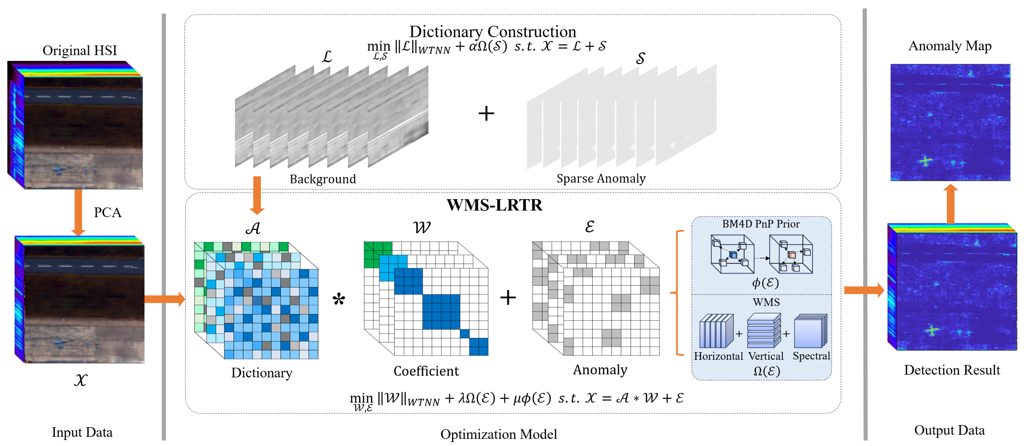
3. The Proposed Method

We initially propose the mathematical formulation by extending structured sparsity to the tensor case, followed by presenting the optimization algorithm in this section.

3.1. New Formulation

For the anomaly E R m 1 × m 2 × m 3 , it can be unfolded from two spatial dimensions and one spectral dimension as:
E ( i ) = u n f o l d ( E , i ) , i = 1 , 2 , 3 ,
where E ( 1 ) R m 2 m 3 × m 1 , E ( 2 ) R m 1 m 3 × m 2 , and E ( 3 ) R m 1 m 2 × m 3 . Then, one can put the resulting three matrices into the structured sparsity to take into account the structured information. For each Ω ( E ( i ) ) , fold it back into the tensor form to get:
E ( i ) = f o l d ( Ω ( E ( i ) ) , i ) , i = 1 , 2 , 3 ,
which allows us to obtain the final WMS by assigning weights to the above tensors, respectively, that is:
Ω ( E ) = γ 1 E ( 1 ) + γ 2 E ( 2 ) + γ 3 E ( 3 ) ,
where γ 1 , γ 2 , γ 3 are three weighting parameters.
In this paper, we refer to this as WMS and show the schematic diagram in Figure 2. By unfolding the anomaly tensor in three dimensions, WMS can effectively extract anomalies from horizontal, vertical, and spectral directions. Specifically, two 2 × 2 sliding blocks of overlapping pixels are used to systematically explore the entire image, and anomalies are then identified by calculating the maximum value within each sliding block. Now, we present the WMS-LRTR model as:
min W , E W WTNN + λ Ω ( E ) + μ ϕ ( E ) s . t . X = A W + E ,
where ϕ ( · ) is the PnP denoising prior [52] and λ , μ are the positive trade-off parameters. Compared with PCA-TLRSR in (11), WMS-LRTR in (16) has two advantages:
  • Ω ( E ) considers the correlation between abnormal pixels across different dimensions and captures multidirectional structured features than E F , 1 , thereby preserving more spatially local anomaly characteristics.
  • ϕ ( E ) complements Ω ( E ) by filtering out noise to preserve the background low-rank structure and facilitate the separation of sparse anomalous regions, thus improving the robustness of AD.

3.2. Optimization Algorithm

This section discusses how to apply the ADMM [61] to solve (16). Two auxiliary variables Z , Y are introduced first, and we reformulate (16) as:
min Z , E , Y , W Z WTNN + λ Ω ( E ) + μ ϕ ( Y ) s . t . X = A W + E , Z = W , Y = E ,
whose augmented Lagrangian function is:
L β ( Z , E , Y , W , Q 1 , Q 2 , Q 3 ) = Z WTNN + λ Ω ( E ) + μ ϕ ( Y ) + Q 1 , X A W E + β 2 X A W E F 2 + Q 2 , Z W + β 2 Z W F 2 + Q 3 , Y E + β 2 Y E F 2 ,
where Q 1 , Q 2 , Q 3 represent the Lagrange multipliers and β > 0 is the penalty parameter. According to the ADMM, Equation (17) can be solved by iteratively updating one variable while keeping the others fixed.
  • The Z -subproblem can be simplified to:
    min Z Z WTNN + β 2 Z W k + Q 2 k β F 2 ,
    where (19) can be addressed using the weighted tensor singular value thresholding according to [58].
  • The E -subproblem can be solved by:
    min E λ Ω ( E ) + β 2 X A W k E + Q 1 k β F 2 + β 2 Y k E + Q 3 k β F 2 ,
    which is equivalent to:
    min E λ Ω ( E ) + β E T k 2 F 2 ,
    where T k = X A W k + Q 1 k β + Y k + Q 3 k β . Then, Equation (21) can be written as:
    min E ( i ) λ Ω ( E ( i ) ) + β E ( i ) T ( i ) k 2 F 2 , i = 1 , 2 , 3 ,
    where E ( i ) = u n f o l d ( E , i ) , i = 1 , 2 , 3 . According to [59], Equation (22) can be solved through the proximal operator. It then follows from the quadratic min-cost flow technique that:
    E ( i ) k + 1 = P r o x ( T ( i ) k 2 , 2 λ β ) , i = 1 , 2 , 3 ,
    then the solution can be obtained by folding E ( i ) and assigning weights to the above tensors, respectively, that is:
    E k + 1 = γ 1 f o l d ( E ( 1 ) k + 1 , 1 ) + γ 2 f o l d ( E ( 2 ) k + 1 , 2 ) + γ 3 f o l d ( E ( 3 ) k + 1 , 3 ) .
  • The Y -subproblem can be rewritten as:
    min Y μ ϕ ( Y ) + β 2 Y E k + 1 + Q 3 k β F 2 ,
    where ϕ ( Y ) is the PnP information, serving as a method for prior denoising supported by BM4D. For convenience, the solution of (25) is given by:
    Y k + 1 = D e n o i s e r ( E k Q 3 k β , μ β ) ,
    where μ β is the noise level.
  • The W -subproblem can be transformed to:
    min W X A W E k + 1 + Q 1 k β F 2 + Z k + 1 W + Q 2 k β F 2 ,
    which can be solved by:
    W k + 1 = ( A A + I ) 1 ( A ( X E k + 1 + Q 1 k β ) + Z k + 1 + Q 2 k β ) ,
    where A is the transpose of A .
  • The Lagrange multipliers Q 1 , Q 2 , Q 3 are updated by:
    Q 1 k + 1 = Q 1 k + β ( X A W k + 1 E k + 1 ) , Q 2 k + 1 = Q 2 k + β ( Z k + 1 W k + 1 ) , Q 3 k + 1 = Q 3 k + β ( Y k + 1 E k + 1 ) , β = min { κ β , β max } .
To sum up, the whole iterative framework is presented in Algorithm 1.
Algorithm 1 Optimization framework
Input: Given data X , dictionary A , parameters λ , μ , β , γ 1 , γ 2 , γ 3 , β max = 10 8 , κ = 1.1 , ϵ = 10 6
Initialize:  Z 0 , L 0 , Y 0 , W 0 , E 0 , Q 1 0 , Q 2 0 , Q 3 0 initialized to 0, set iteration number k = 0
While not converged do
   1:
Update Z k + 1 by weighted tensor singular value thresholding [58]
   2:
Update E k + 1 by (24)
   3:
Update Y k + 1 by (26)
   4:
Update W k + 1 by (28)
   5:
Update Q 1 k + 1 , Q 2 k + 1 , Q 3 k + 1 by (29)
   6:
check convergence:
max Z k + 1 Z k , E k + 1 E k , Y k + 1 Y k , W k + 1 W k ϵ
   7:
k = k + 1
End While
Output:  E

3.3. Dictionary Construction

In LRTR-based AD methods, the quality of the background dictionary is important for enhancing AD accuracy. Some existing methods regard the entire HSI as a dictionary, and this construction method usually has two drawbacks [62,63]. First, the dictionary contains too many elements, resulting in significant computational overhead. Second, HSI is inevitably affected by noise during the acquisition and transmission. Therefore, we perform PCA preprocessing on the HSI tensor before dictionary construction to reduce both the computational burden and the impact of noisy bands. Tensor robust principal component analysis (TRPCA) [57] utilizes the tensor nuclear norm and and L 1 -norm to decompose the input data tensor into low-rank and sparse tensors. Inspired by TRPCA, our dictionary construction strategy employs WTNN appropriately allocate the singular value weights to preserve the low-rank characteristics of the background, while Ω ( S ) is used to merge the abnormal pixels of each band from spatial and spectral dimensions, enhancing anomaly sparsity and resulting in a cleaner background:
min L , S L WTNN + α Ω ( S ) s . t . X = L + S ,
where α is the positive trade-off parameter, L is the low-rank background, and S is the sparse anomaly. Equation (30) is solved using ADMM with the augmented Lagrangian function given by:
L β ( L , S , Q 4 ) = L WTNN + α Ω ( S ) + Q 4 , X L S + β 2 X L S F 2 ,
where Q 4 represents the Lagrange multiplier and β > 0 is the penalty parameter. Equation (31) can be solved in a similar way as in Section 3.2.
  • The L -subproblem can be simplified to:
    min L L WTNN + β 2 X L S k + Q 4 k β F 2 ,
    where the solution of (32) is similar to (19).
  • The S -subproblem can be simplified to:
    min S α Ω ( S ) + β 2 X L k S + Q 4 k β F 2 ,
    which has a closed-form solution similar to (22).
  • The Lagrange multipliers Q 4 is updated by:
    Q 4 k + 1 = Q 4 k + β ( X L k + 1 S k + 1 ) , β = min { κ β , β max } .
The resulting background component L is then used as the constructed dictionary A , i.e., A = L . This construction strategy is based on LRTR, and the resulting tensor dictionary A preserves the inherent spatial–spectral structure.

4. Experiments and Discussions

In this section, WMS-LRTR is compared with nine benchmark methods, including RX [14], LRASR [26], GTVLRR [28], AUTO-AD [43], RGAE [44], DeCNN-AD [53], PTA [36], PCA-TLRSR [37], and LARTVAD [38]. Among them, RX, LRASR, and GTVLRR are three classical methods, and others are proposed in recent years. All experiments in this paper are performed on Matlab R2018a and Pytorch 1.9.0 on a computer with Intel i5-10210U CPU@1.60 GHz and 12 GB RAM in Windows 10.

4.1. Dataset Description

To evaluate the effectiveness of WMS-LRTR, thirteen datasets from Airport–Beach–Urban (ABU) database are considered. ABU was captured by the airborne visible/infrared imaging spectrometer (AVIRIS) sensor and the reflective optics system imaging spectrometer (ROSIS) sensor and contains three subscenes in total: airport, beach, and urban, see Figure 3. The size is 100 × 100 × N or 150 × 150 × N , where N is in the range from 102 to 207. The details of these datasets are listed in Table 1.

4.2. Implementation Details

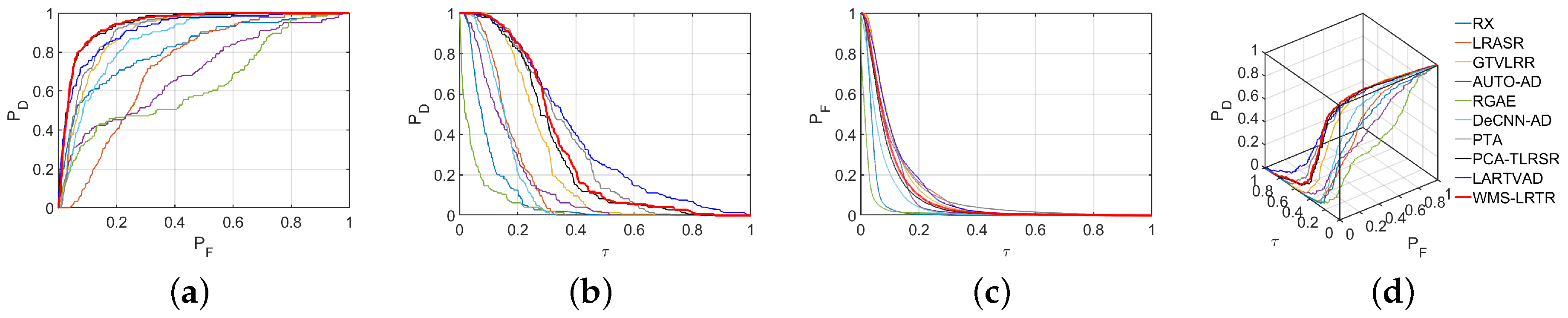
4.2.1. Performance Indicators

In this paper, we employ three commonly used evaluation metrics, namely, AD map, 3D receiver operating characteristic (ROC) curve [64], and area under the ROC curve (AUC). The interplay among detection probability P D , false alarm probability P F , and detection threshold τ is depicted by the 3D ROC curve. Furthermore, three 2D ROC curves representing ( P D , P F ), ( P D , τ ), and ( P F , τ ) can be obtained from the 3D ROC curve. The ROC curve of ( P D , P F ) is near the upper left corner and ( P D , τ ) is near the upper right corner, indicating better detection performance. On the contrary, the ROC curve of ( P F , τ ) is close to the lower left corner, indicating a stronger ability to suppress the background. Consequently, we can derive AUC ( D , F ) , AUC ( D , τ ) , and AUC ( F , τ ) from these curves. Integrating these evaluation indicators with each other, the following four comprehensive evaluation indicators can be obtained, which are, respectively, called AUC TD , AUC BS , AUC TDBS , and AUC ODP . Typically, AUC ( D , F ) and AUC TDBS are used to assess the efficiency of the detector, while AUC ODP assesses the overall detection performance. These three indicators are considered the most important. Moreover, AUC ( D , τ ) and AUC TD evaluate the target detection capability. AUC ( F , τ ) and AUC BS evaluate the background suppression capability.

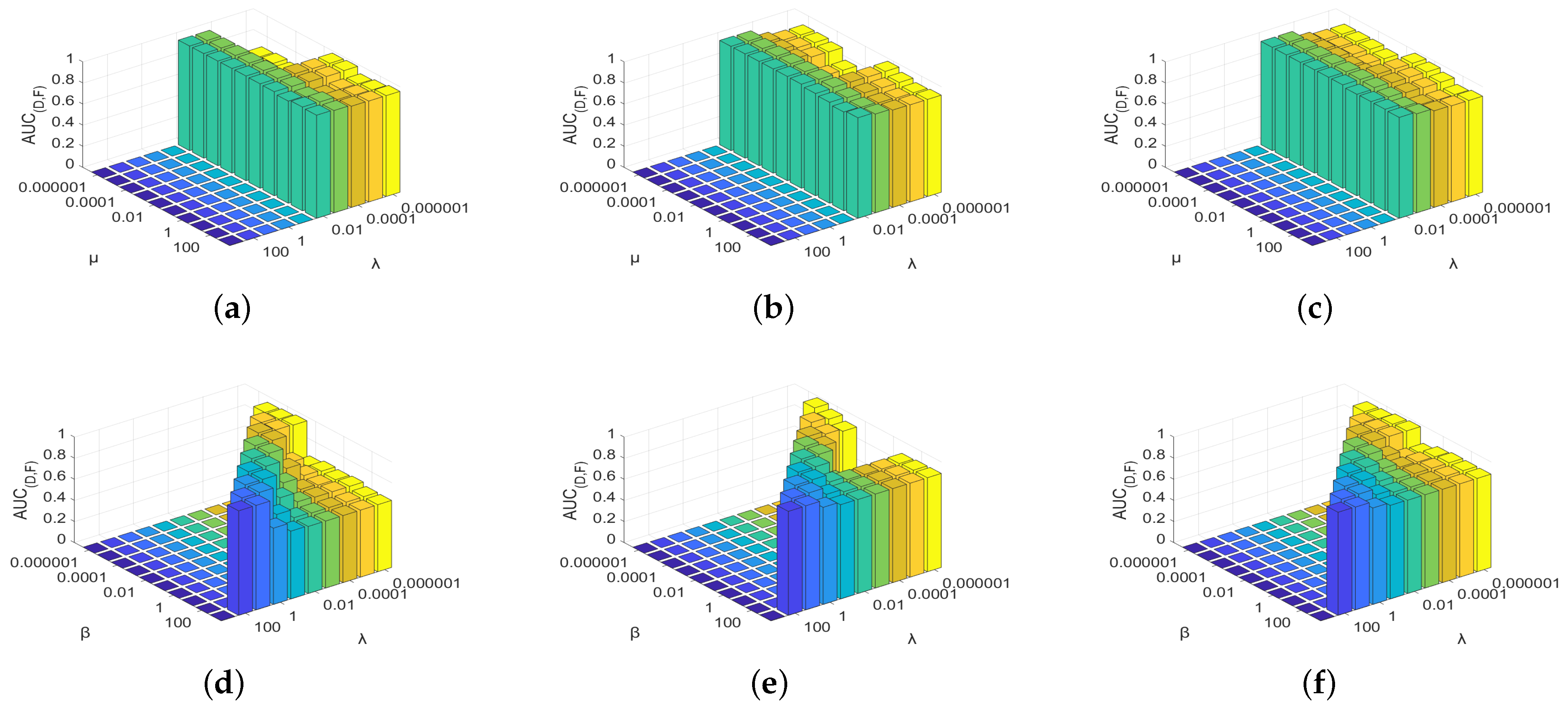
4.2.2. Parameter Selection

In WMS-LRTR, there exist three parameters, i.e., λ , μ , and β . Their variation range is set from 10 6 to 10 4 . The AUC ( D , F ) changes under different parameter settings on Urban-3, Urban-4, and Urban-5 are shown in Figure 4a–f, respectively. Then, we discuss the selection of spectral dimensions for PCA. Figure 5 illustrates the AUC ( D , F ) values vary with the spectral dimension. The best spectral dimensions for the thirteen datasets are 4, 5, 12, 5, 12, 12, 11, 12, 8, 8, 4, 6, and 8, respectively. In all experiments, when { λ , μ , β } are set to { 10 2 , 10 2 , 10 1 }, WMS-LRTR exhibits the superior performance. For convenience, γ 1 , γ 2 , γ 3 are set to 1 / 3 . The parameters of the compared methods are set to the optimal values recommended in the respective literature. For LRASR, the number of clusters K is set to 15, with each cluster containing 20 atoms. The parameters λ and β are varied within the range of 0.01 to 1. For GTVLRR, the parameters λ , β , and γ are set to 0.05, 0.2, and 0.02, respectively. The trade-off parameter λ , the number of superpixels S, and the dimension of the hidden layer n _ h i d in RGAE are set to 0.01, 150, and 100, respectively. The parameters of DeCNN-AD are K, β , and λ and we set them to 5, 0.1, and 0.1. For PTA, the truncated low-rank r, α , and τ are set to 1, 1, and 0.01, respectively, while μ is chosen from the range 0.1 to 0.5. The parameters in PCA-TLRSR are set based on the recommendations provided in [37]. For the parameters K, β , and λ in LARTVAD, we set them to 80, 0.1, and 1, respectively.

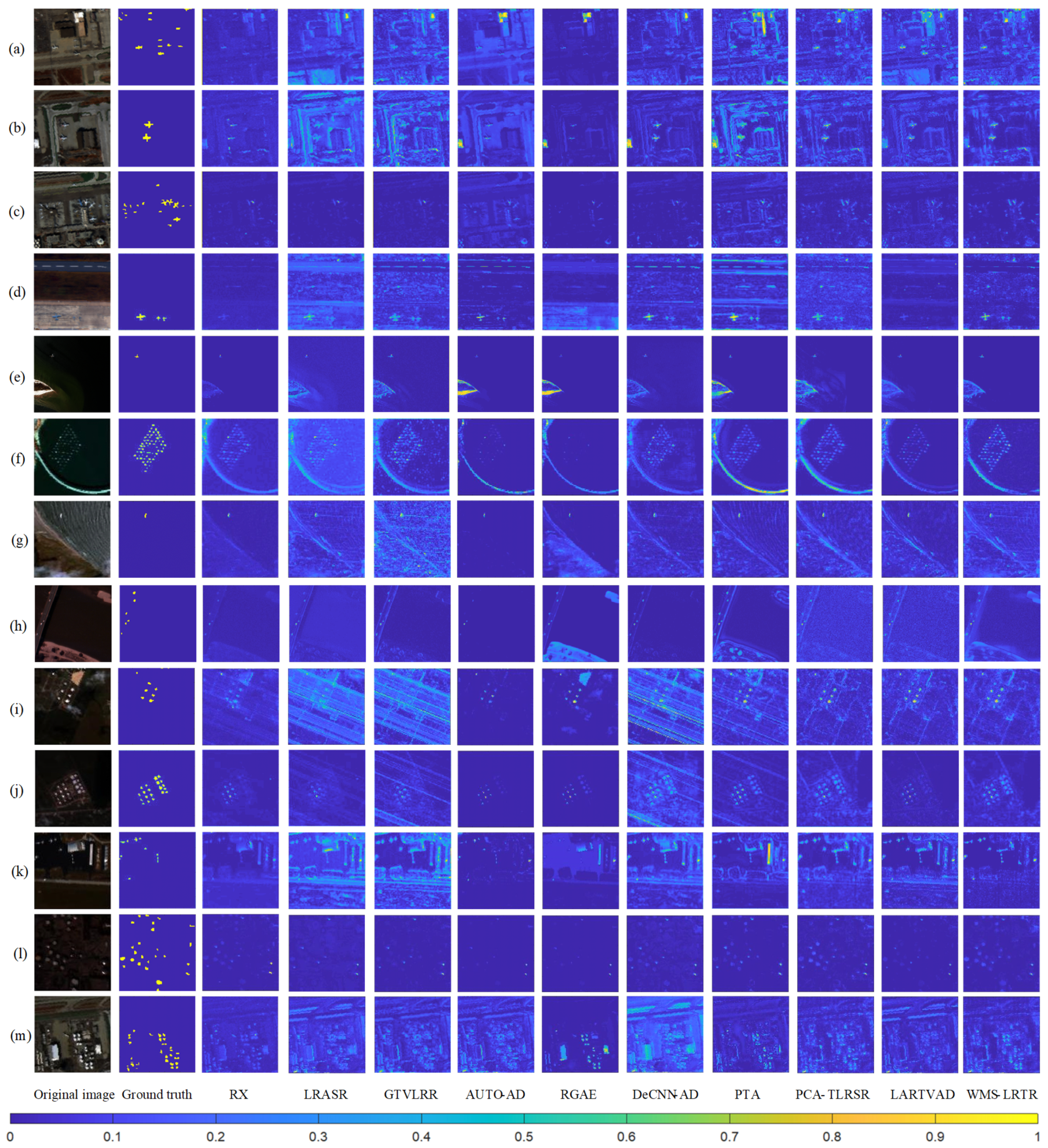
4.3. Numerical Results

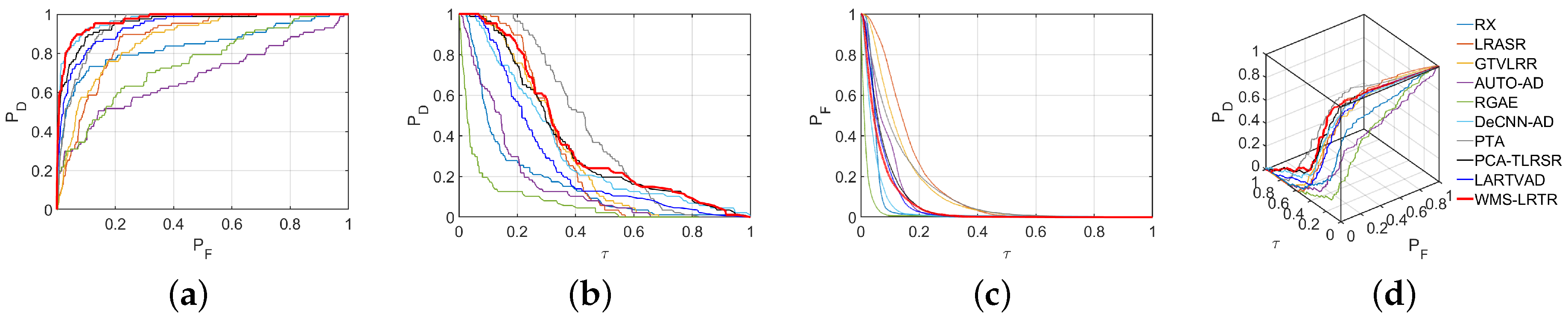
4.3.1. Experiments on the Airport Scenes

Figure 3 illustrates the AD maps for all the compared methods on the Airport scenes. Among all the methods, RX, LRASR, and GTVLRR detect fewer anomalies. AUTO-AD and RGAE demonstrate strong background suppression capabilities, but their detection performance is not excellent. PTA shows better detection ability but tends to generate redundant background components in the AD map. Among the remaining methods, the proposed WMS-LRTR successfully detects more anomalies while effectively suppressing the background.
In addition, the ROC curves for Airport-1 and Airport-2 are shown in Figure 6 and Figure 7. As can be seen in Figure 6a and Figure 7a, WMS-LRTR surpasses all methods to achieve the best performance. In Figure 6b and Figure 7b, WMS-LRTR shows slightly inferior to PTA. However, in Figure 6c and Figure 7c, PTA performs significantly worse than WMS-LRTR. Therefore, as demonstrated in Figure 6d and Figure 7d, WMS-LRTR exhibits better overall performance compared to all other methods. Additionally, Table 2 shows the AUC values for all methods on the Airport scenes. As can be seen from Table 2, for AUC ( D , F ) , which evaluates detector efficiency, WMS-LRTR outperforms all other methods, achieving the highest value across the four datasets. Besides, for AUC ODP , which assesses overall performance, WMS-LRTR achieves either the best or the second-best value across the datasets, further demonstrating its effectiveness.

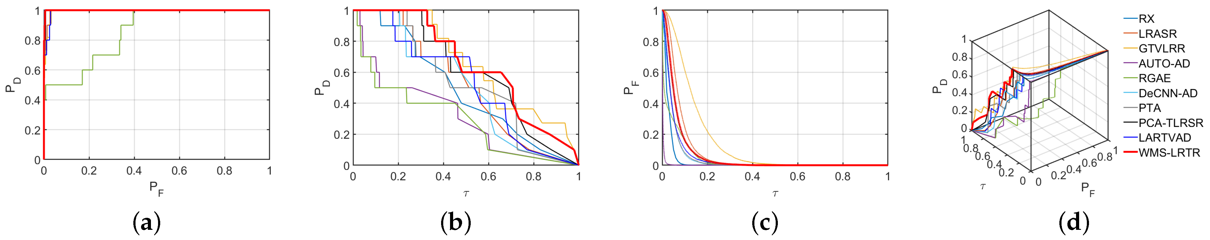
4.3.2. Experiments on the Beach Scenes

Figure 3 depicts the visualization maps of compared methods on the Beach scenes. For Beach-1 and Beach-2, AUTO-AD and RGAE perform poorly, while other methods are able to identify the majority of the anomalies. Among these methods, WMS-LRTR exhibits better background suppression ability and detection efficiency. For Beach-3 and Beach-4, AUTO-AD based on deep learning shows excellent background suppression ability. Among the other methods, anomalies detected by WMS-LRTR are obvious, although it should be acknowledged that its background suppression ability is slightly weaker than AUTO-AD.
Figure 8 and Figure 9 give the related ROC curves on Beach-2 and Beach-3. In Figure 8a,b and Figure 9a,b, the ROC curve of WMS-LRTR is closest to the upper left and right corners, respectively. In Figure 8c and Figure 9c, WMS-LRTR is slightly inferior to AUTO-AD and RGAE. Besides, the AUC values on the Beach scenes are provided in Table 3. As shown in Table 3, both AUC ( D , F ) and AUC ODP achieve either the best or suboptimal performance across the four datasets, further demonstrating the better efficiency and overall detection capability of WMS-LRTR.

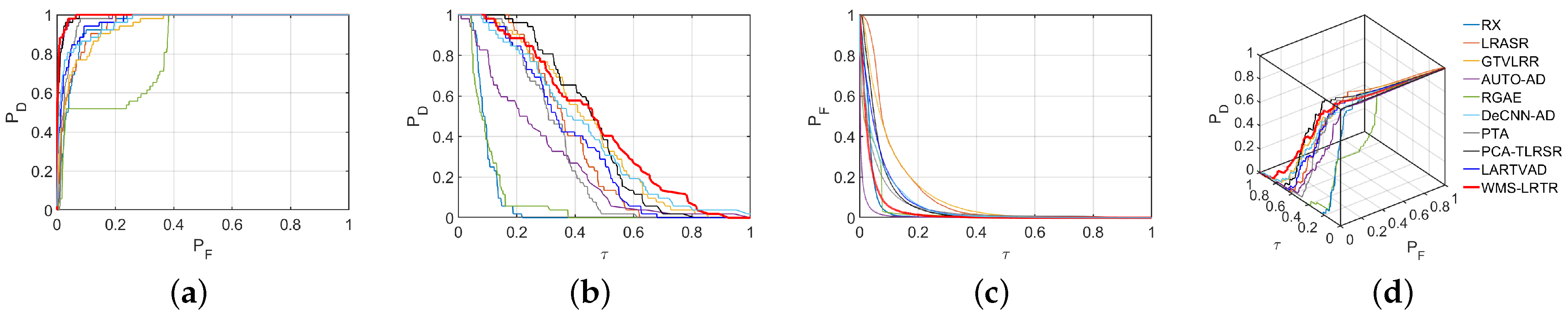
4.3.3. Experiments on the Urban Scenes

Figure 3 shows the detection visual results for the Urban scenes. AUTO-AD and RGAE exhibit good background suppression ability on these five datasets, but they fail to detect all anomalies or mistakenly classify background pixels as anomalies. LRASR, GTVLRR, and DeCNN-AD mistakenly identify more background as abnormal targets, resulting in a poorer visual effect. RX and LARTVAD do not perform well in AD, as many anomalies are not detected. PTA, PCA-TLRSR, and WMS-LRTR are able to detect all anomalies Compared with the previous two methods, WMS-LRTR exhibits better detection effectiveness and identifies fewer background pixels as anomalies.
The ROC curves of the Urban scenes are shown in Figure 10, Figure 11, Figure 12, Figure 13 and Figure 14. From the ROC curves of ( P D , P F ) on these datasets, WMS-LRTR is consistently in the upper left corner, indicating its significantly superior performance compared to other methods. Besides, there is a crossover between WMS-LRTR and other methods for the ROC curves of ( P D , τ ), but WMS-LRTR is the closest to the upper right corner. WMS-LRTR performs slightly worse than AUTO-AD and RGAE for the ROC curves of ( P F , τ ), but these two methods show poorer performance on the other ROC curves. From Figure 10c, Figure 11c, Figure 12c, Figure 13c and Figure 14c, it is evident that the ROC curve of WMS-LRTR consistently appears in the lower left corner across these five datasets, which demonstrates that WMS-LRTR maintains a low false alarm rate across different threshold τ . In addition, all AUC values are presented in Table 4. For AUC ( D , F ) , which evaluates the effectiveness of detectors, WMS-LRTR obtains the optimal value on the five datasets. For AUC ODP , which evaluates the overall detection performance, WMS-LRTR also achieves the optimal value on all datasets. Finally, Table 5 presents the average AUC values across the thirteen datasets. Except for AUC ( F , τ ) , all other indicators show that WMS-LRTR achieved the best values. Furthermore, the AUC ( D , F ) is increased by about 1.6% compared to PCA-TLRSR. These quantitative experimental results clearly demonstrate the superiority of WMS-LRTR over other competing methods.

4.4. Discussion

4.4.1. Statistical Separability Analysis

In this section, we utilize boxplots to visualize ability of WMS-LRTR to distinguish anomalies from the background. The resulting boxplots are shown in Figure 15, where the green box illustrates the distribution of the background, and the red box represents the distribution of the anomalies. The distance between the two boxes serves as an intuitive indicator of the ability to separate anomalies from the background. A larger distance between the two boxes indicates better AD ability. For Urban-1, Urban-3, and Urban-5, WMS-LRTR has the best ability to separate anomaly and background. For Airport-1 and Beach-2, all methods exhibit poor separation, but WMS-LRTR still achieves the best performance. However, for Beach-3, Urban-2, and Urban-4, the separation capability of WMS-LRTR is slightly lower than AUTO-AD and RGAE, resulting in a suboptimal result. In summary, the proposed WMS-LRTR method demonstrates a better capability for separating anomalies from the background.

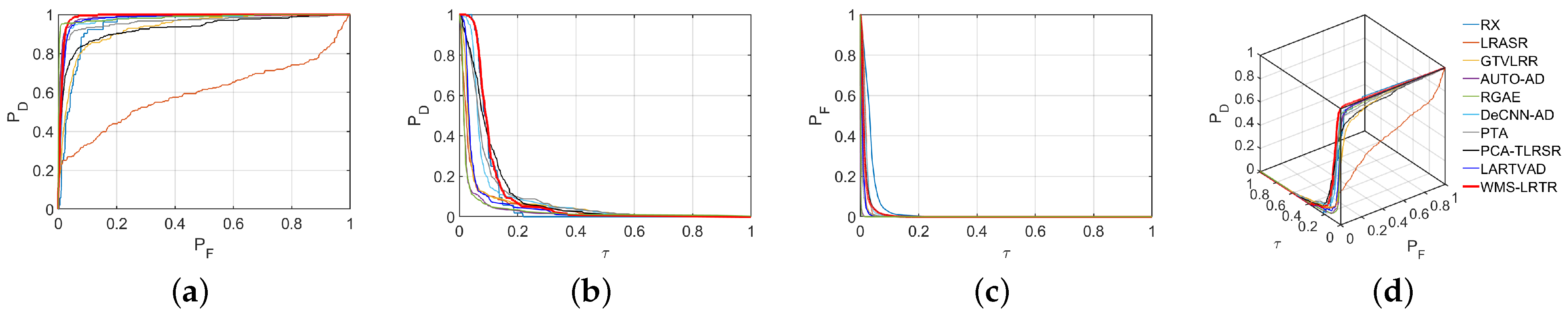
4.4.2. Noise Resistance Analysis

This section discusses the noise resistance ability of WMS-LRTR. In the experiment, we apply Gaussian noise with a density of 0.2 to each band and randomly select 20 bands with a density of 0.2 salt and pepper noise to generate two synthetic datasets, called Noisy Beach-3 and Noisy Urban-3. The visualization results are depicted in Figure 16, with the corresponding AUC values provided in Table 6. The detection maps of WMS-LRTR are closest to the ground truth, with PTA achieving the second-best performance. In addition, the other methods exhibit poor performance, being severely affected by noise, and detect almost no anomalies. As shown in Table 6, WMS-LRTR achieves a relatively high AUC ( D , F ) and AUC ODP value even in the presence of severe noise interference. In addition, in noisy environments, WMS-LRTR demonstrates the best background suppression ability, with both AUC ( F , τ ) and AUC BS achieving optimal values, which can be attributed to the PnP denoising prior. On the two noisy datasets, the AUC ( D , F ) of WMS-LRTR is higher by 0.2% and 2.2% compared to the second-best PTA method. In summary, the proposed WMS-LRTR method has excellent noise resistance ability and still maintains superior AD performance even in severe noisy cases.

4.4.3. Ablation Analysis

Ablation experiments are carried out on four datasets in this section. Table 7 summarizes the AUC ( D , F ) values without PCA, WTNN, WMS, and PnP denoising prior, respectively. In the case without WMS, we apply the L F , 1 -norm which can explore tensor sparsity as an alternative. As shown in Table 7, AUC ( D , F ) of WMS-LRTR is higher by 3.3%, 3.6%, 0.5%, and 1.5%, respectively, in the four cases, which convinces the effectiveness of WMS-LRTR. In addition, the corresponding runtime is also provided in Table 7, from which it is evident that PCA significantly reduces the computational load required for detection. This is the reason why we employ PCA as a data preprocessing step.
Moreover, Table 8 further demonstrates the superiority of WMS. We compare the AUC ( D , F ) results of WMS with those obtained by considering only a single direction, respectively. Since WMS simultaneously explores the sparsity of abnormal local structural features from three dimensions, horizontal, vertical, and spectral, and considers the spatial characteristics of HSI, it achieves better results than only considering one direction.
In addition, Table 9 presents the runtime in seconds of compared methods. It can be seen that the runtime of WMS-LRTR is slightly slower, primarily due to the computational overhead caused by WMS and PnP denoising. Nonetheless, WMS-LRTR demonstrates superior detection ability compared to other methods. Therefore, although there is a trade-off in execution time, the performance improvement justifies this compromise within reasonable limits.

4.4.4. Block Size Analysis

This section discusses the configuration of the block size involved in WMS. As shown in Table 10, increasing the block size does not lead to a significant improvement in detection capability. On the contrary, as the block size increases, the number of pixels involved in each calculation grows, resulting in a heavier computational burden. Therefore, considering both detection performance and computational time, we set the block size to 2 × 2 .

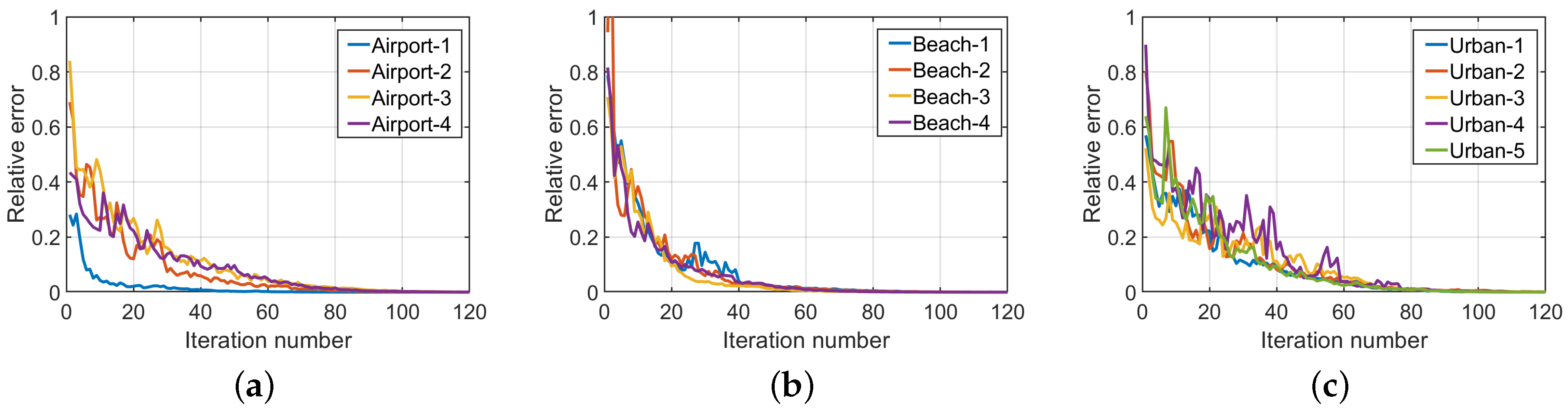
4.4.5. Convergence Analysis

This section presents the relative errors with the number of iterations on all selected datasets. It follows from Figure 17 that fluctuations in the relative errors are observed within the initial 40 iterations, and the convergence curves gradually become smoother in the subsequent iterations. Furthermore, the relative errors approach zero within 100 iterations for all datasets. This observation further validates the convergence capability of WMS-LRTR.

5. Conclusions

This paper introduces a WMS-LRTR method for AD. Specifically, WTNN estimates the background effectively, WMS can exploit the local structure through tensor unfolding, while PnP denoising prior can effectively preserve low-rank property of the background. By integrating them in a tensor approximation framework, we ensure the low-rank property of the background, local structured sparsity of the anomaly, and the robustness of AD. Comprehensive experiments with nine methods on eight datasets demonstrate that WMS-LRTR outperforms the others, with the average AUC ( D , F ) increased by approximately 1.6% compared to the second-best PCA-TLRSR method. Moreover, the statistical separability, noise resistance, ablation, and convergence have been discussed in detail.
Although WMS-LRTR achieves better detection results, it often takes more time. In the future, we are interested in developing faster optimization algorithms to reduce the computational cost. In addition, we will combine it with advanced deep learning methods to further improve the performance.

Author Contributions

J.L., J.J. and X.X. completed the methodology, collected the experimental data, and wrote the manuscript. J.L., X.X., W.L. and J.Z. completed the checking and revision of the manuscript. All authors have read and agreed to the published version of the manuscript.

Funding

This work was supported in part by the National Natural Science Foundation of China under Grant 62204044 and 12371306, and in part by the State Key Laboratory of Integrated Chips and Systems under Grant SKLICS-K202302.

Data Availability Statement

Datasets are available at http://xudongkang.weebly.com/data-sets.html (accessed on 11 January 2013). Our codes will be available at https://github.com/Jason011212 (accessed on 5 February 2025).

Conflicts of Interest

The authors declare no conflicts of interest.

References

  1. Zhang, H.; Chen, H.; Yang, G.; Zhang, L. LR-Net: Low-Rank Spatial-Spectral Network for Hyperspectral Image Denoising. IEEE Trans. Image Process. 2021, 30, 8743–8758. [Google Scholar] [CrossRef] [PubMed]
  2. Zhuang, L.; Ng, M.K.; Gao, L.; Wang, Z. Eigen-CNN: Eigenimages Plus Eigennoise Level Maps Guided Network for Hyperspectral Image Denoising. IEEE Trans. Geosci. Remote Sens. 2024, 62, 5512018. [Google Scholar] [CrossRef]
  3. Zhang, Q.; Zheng, Y.; Yuan, Q.; Song, M.; Yu, H.; Xiao, Y. Hyperspectral Image Denoising: From Model-Driven, Data-Driven, to Model-Data-Driven. IEEE Trans. Neural Netw. Learn. Syst. 2024, 35, 13143–13163. [Google Scholar] [CrossRef]
  4. Dong, Y.; Shi, W.; Du, B.; Hu, X.; Zhang, L. Asymmetric Weighted Logistic Metric Learning for Hyperspectral Target Detection. IEEE Trans. Cybern. 2022, 52, 11093–11106. [Google Scholar] [CrossRef] [PubMed]
  5. Li, C.; Zhang, B.; Hong, D.; Yao, J.; Chanussot, J. LRR-Net: An Interpretable Deep Unfolding Network for Hyperspectral Anomaly Detection. IEEE Trans. Geosci. Remote Sens. 2023, 61, 5513412. [Google Scholar] [CrossRef]
  6. Chang, C.I.; Chen, S.; Zhong, S.; Shi, Y. Exploration of Data Scene Characterization and 3D ROC Evaluation for Hyperspectral Anomaly Detection. Remote Sens. 2024, 16, 135. [Google Scholar] [CrossRef]
  7. Han, Y.; Zhu, H.; Jiao, L.; Yi, X.; Li, X.; Hou, B.; Ma, W.; Wang, S. SSMU-Net: A Style Separation and Mode Unification Network for Multimodal Remote Sensing Image Classification. IEEE Trans. Geosci. Remote Sens. 2023, 61, 5407115. [Google Scholar] [CrossRef]
  8. Chen, H.; Ru, J.; Long, H.; He, J.; Chen, T.; Deng, W. Semi-Supervised Adaptive Pseudo-Label Feature Learning for Hyperspectral Image Classification in Internet of Things. IEEE Internet Things J. 2024, 11, 30754–30768. [Google Scholar] [CrossRef]
  9. Huang, S.; Liu, Z.; Jin, W.; Mu, Y. Superpixel-based multi-scale multi-instance learning for hyperspectral image classification. Pattern Recognit. 2024, 149, 110257. [Google Scholar]
  10. Gao, H.; Li, S.; Dian, R. Hyperspectral and Multispectral Image Fusion Via Self-Supervised Loss and Separable Loss. IEEE Trans. Geosci. Remote Sens. 2022, 60, 5537712. [Google Scholar] [CrossRef]
  11. Wang, X.; Wang, X.; Zhao, K.; Zhao, X.; Song, C. FSL-Unet: Full-Scale Linked Unet With Spatial–Spectral Joint Perceptual Attention for Hyperspectral and Multispectral Image Fusion. IEEE Trans. Geosci. Remote Sens. 2022, 60, 5539114. [Google Scholar] [CrossRef]
  12. Li, H.C.; Feng, X.R.; Wang, R.; Gao, L.; Du, Q. Superpixel-Based Low-Rank Tensor Factorization for Blind Nonlinear Hyperspectral Unmixing. IEEE Sens. J. 2024, 24, 13055–13072. [Google Scholar] [CrossRef]
  13. Li, M.; Yang, B.; Wang, B. EMLM-Net: An Extended Multilinear Mixing Model-Inspired Dual-Stream Network for Unsupervised Nonlinear Hyperspectral Unmixing. IEEE Trans. Geosci. Remote Sens. 2024, 62, 5509116. [Google Scholar] [CrossRef]
  14. Reed, I.; Yu, X. Adaptive multiple-band CFAR detection of an optical pattern with unknown spectral distribution. IEEE Trans. Acoust. Speech Signal Process. 1990, 38, 1760–1770. [Google Scholar] [CrossRef]
  15. Chang, C.I.; Chiang, S.S. Anomaly detection and classification for hyperspectral imagery. IEEE Trans. Geosci. Remote Sens. 2002, 40, 1314–1325. [Google Scholar] [CrossRef]
  16. Kwon, H.; Nasrabadi, N. Kernel RX-algorithm: A nonlinear anomaly detector for hyperspectral imagery. IEEE Trans. Geosci. Remote Sens. 2005, 43, 388–397. [Google Scholar] [CrossRef]
  17. Guo, Q.; Zhang, B.; Ran, Q.; Gao, L.; Li, J.; Plaza, A. Weighted-RXD and Linear Filter-Based RXD: Improving Background Statistics Estimation for Anomaly Detection in Hyperspectral Imagery. IEEE J. Sel. Top. Appl. Earth Obs. Remote Sens. 2014, 7, 2351–2366. [Google Scholar] [CrossRef]
  18. Zhou, J.; Kwan, C.; Ayhan, B.; Eismann, M.T. A Novel Cluster Kernel RX Algorithm for Anomaly and Change Detection Using Hyperspectral Images. IEEE Trans. Geosci. Remote Sens. 2016, 54, 6497–6504. [Google Scholar] [CrossRef]
  19. Ren, L.; Zhao, L.; Wang, Y. A Superpixel-Based Dual Window RX for Hyperspectral Anomaly Detection. IEEE Geosci. Remote Sens. Lett. 2020, 17, 1233–1237. [Google Scholar] [CrossRef]
  20. Donoho, D. Compressed sensing. IEEE Trans. Inf. Theory 2006, 52, 1289–1306. [Google Scholar] [CrossRef]
  21. Liu, G.; Lin, Z.; Yan, S.; Sun, J.; Yu, Y.; Ma, Y. Robust Recovery of Subspace Structures by Low-Rank Representation. IEEE Trans. Pattern Anal. Mach. Intell. 2013, 35, 171–184. [Google Scholar] [CrossRef]
  22. Chen, Y.; Nasrabadi, N.M.; Tran, T.D. Sparse Representation for Target Detection in Hyperspectral Imagery. IEEE J. Sel. Top. Signal Process. 2011, 5, 629–640. [Google Scholar] [CrossRef]
  23. Li, J.; Zhang, H.; Zhang, L.; Ma, L. Hyperspectral Anomaly Detection by the Use of Background Joint Sparse Representation. IEEE J. Sel. Top. Appl. Earth Obs. Remote Sens. 2015, 8, 2523–2533. [Google Scholar] [CrossRef]
  24. Ling, Q.; Guo, Y.; Lin, Z.; An, W. A Constrained Sparse Representation Model for Hyperspectral Anomaly Detection. IEEE Trans. Geosci. Remote Sens. 2019, 57, 2358–2371. [Google Scholar] [CrossRef]
  25. Qin, H.; Shen, Q.; Zeng, H.; Chen, Y.; Lu, G. Generalized Nonconvex Low-Rank Tensor Representation for Hyperspectral Anomaly Detection. IEEE Trans. Geosci. Remote Sens. 2023, 61, 5526612. [Google Scholar] [CrossRef]
  26. Xu, Y.; Wu, Z.; Li, J.; Plaza, A.; Wei, Z. Anomaly Detection in Hyperspectral Images Based on Low-Rank and Sparse Representation. IEEE Trans. Geosci. Remote Sens. 2016, 54, 1990–2000. [Google Scholar] [CrossRef]
  27. Zhang, Y.; Du, B.; Zhang, L.; Wang, S. A Low-Rank and Sparse Matrix Decomposition-Based Mahalanobis Distance Method for Hyperspectral Anomaly Detection. IEEE Trans. Geosci. Remote Sens. 2016, 54, 1376–1389. [Google Scholar] [CrossRef]
  28. Cheng, T.; Wang, B. Graph and Total Variation Regularized Low-Rank Representation for Hyperspectral Anomaly Detection. IEEE Trans. Geosci. Remote Sens. 2020, 58, 391–406. [Google Scholar] [CrossRef]
  29. Shen, X.; Liu, H.; Nie, J.; Zhou, X. Matrix Factorization With Framelet and Saliency Priors for Hyperspectral Anomaly Detection. IEEE Trans. Geosci. Remote Sens. 2023, 61, 5504413. [Google Scholar] [CrossRef]
  30. Lin, J.T.; Lin, C.H. SuperRPCA: A Collaborative Superpixel Representation Prior-Aided RPCA for Hyperspectral Anomaly Detection. IEEE Trans. Geosci. Remote Sens. 2024, 62, 5532516. [Google Scholar] [CrossRef]
  31. Zhang, X.; Wen, G.; Dai, W. A Tensor Decomposition-Based Anomaly Detection Algorithm for Hyperspectral Image. IEEE Trans. Geosci. Remote Sens. 2016, 54, 5801–5820. [Google Scholar] [CrossRef]
  32. Zhou, P.; Lu, C.; Feng, J.; Lin, Z.; Yan, S. Tensor Low-Rank Representation for Data Recovery and Clustering. IEEE Trans. Pattern Anal. Mach. Intell. 2021, 43, 1718–1732. [Google Scholar] [CrossRef]
  33. A, R.; Mu, X.; He, J. Enhance Tensor RPCA-Based Mahalanobis Distance Method for Hyperspectral Anomaly Detection. IEEE Geosci. Remote Sens. Lett. 2022, 19, 6008305. [Google Scholar] [CrossRef]
  34. Shang, W.; Jouni, M.; Wu, Z.; Xu, Y.; Dalla Mura, M.; Wei, Z. Hyperspectral Anomaly Detection Based on Regularized Background Abundance Tensor Decomposition. Remote Sens. 2023, 15, 1679. [Google Scholar] [CrossRef]
  35. Sun, S.; Liu, J.; Zhang, Z.; Li, W. Hyperspectral Anomaly Detection Based on Adaptive Low-Rank Transformed Tensor. IEEE Trans. Neural Netw. Learn. Syst. 2024, 35, 9787–9799. [Google Scholar] [CrossRef]
  36. Li, L.; Li, W.; Qu, Y.; Zhao, C.; Tao, R.; Du, Q. Prior-Based Tensor Approximation for Anomaly Detection in Hyperspectral Imagery. IEEE Trans. Neural Netw. Learn. Syst. 2022, 33, 1037–1050. [Google Scholar] [CrossRef] [PubMed]
  37. Wang, M.; Wang, Q.; Hong, D.; Roy, S.K.; Chanussot, J. Learning Tensor Low-Rank Representation for Hyperspectral Anomaly Detection. IEEE Trans. Cybern. 2023, 53, 679–691. [Google Scholar] [CrossRef]
  38. Sun, S.; Liu, J.; Chen, X.; Li, W.; Li, H. Hyperspectral Anomaly Detection With Tensor Average Rank and Piecewise Smoothness Constraints. IEEE Trans. Neural Netw. Learn. Syst. 2023, 34, 8679–8692. [Google Scholar] [CrossRef] [PubMed]
  39. Feng, M.; Chen, W.; Yang, Y.; Shu, Q.; Li, H.; Huang, Y. Hyperspectral Anomaly Detection Based on Tensor Ring Decomposition With Factors TV Regularization. IEEE Trans. Geosci. Remote Sens. 2023, 61, 5514114. [Google Scholar] [CrossRef]
  40. Ren, L.; Gao, L.; Wang, M.; Sun, X.; Chanussot, J. HADGSM: A Unified Nonconvex Framework for Hyperspectral Anomaly Detection. IEEE Trans. Geosci. Remote Sens. 2024, 62, 5503415. [Google Scholar] [CrossRef]
  41. Xiao, Q.; Zhao, L.; Chen, S.; Li, X. Robust Tensor Low-Rank Sparse Representation With Saliency Prior for Hyperspectral Anomaly Detection. IEEE Trans. Geosci. Remote Sens. 2023, 61, 5529920. [Google Scholar] [CrossRef]
  42. Cheng, X.; Mu, R.; Lin, S.; Zhang, M.; Wang, H. Hyperspectral Anomaly Detection via Low-Rank Representation with Dual Graph Regularizations and Adaptive Dictionary. Remote Sens. 2024, 16, 1837. [Google Scholar] [CrossRef]
  43. Wang, S.; Wang, X.; Zhang, L.; Zhong, Y. Auto-AD: Autonomous Hyperspectral Anomaly Detection Network Based on Fully Convolutional Autoencoder. IEEE Trans. Geosci. Remote Sens. 2022, 60, 5503314. [Google Scholar] [CrossRef]
  44. Fan, G.; Ma, Y.; Mei, X.; Fan, F.; Huang, J.; Ma, J. Hyperspectral Anomaly Detection With Robust Graph Autoencoders. IEEE Trans. Geosci. Remote Sens. 2022, 60, 5511314. [Google Scholar] [CrossRef]
  45. Xiang, P.; Ali, S.; Jung, S.K.; Zhou, H. Hyperspectral Anomaly Detection With Guided Autoencoder. IEEE Trans. Geosci. Remote Sens. 2022, 60, 5538818. [Google Scholar] [CrossRef]
  46. Mu, Z.; Wang, Y.; Zhang, Y.; Song, C.; Wang, X. MPDA: Multivariate Probability Distribution Autoencoder for Hyperspectral Anomaly Detection. IEEE Trans. Geosci. Remote Sens. 2024, 62, 5538513. [Google Scholar] [CrossRef]
  47. Liu, H.; Su, X.; Shen, X.; Zhou, X. MSNet: Self-Supervised Multiscale Network With Enhanced Separation Training for Hyperspectral Anomaly Detection. IEEE Trans. Geosci. Remote Sens. 2024, 62, 5520313. [Google Scholar] [CrossRef]
  48. Wang, X.; Chen, J.; Richard, C. Tuning-Free Plug-and-Play Hyperspectral Image Deconvolution With Deep Priors. IEEE Trans. Geosci. Remote Sens. 2023, 61, 5506413. [Google Scholar] [CrossRef]
  49. He, Y.; Zhang, C.; Zhang, B.; Chen, Z. FSPnP: Plug-and-Play Frequency–Spatial-Domain Hybrid Denoiser for Thermal Infrared Image. IEEE Trans. Geosci. Remote Sens. 2024, 62, 5000416. [Google Scholar] [CrossRef]
  50. Zhuang, L.; Bioucas-Dias, J.M. Fast Hyperspectral Image Denoising and Inpainting Based on Low-Rank and Sparse Representations. IEEE J. Sel. Top. Appl. Earth Obs. Remote Sens. 2018, 11, 730–742. [Google Scholar] [CrossRef]
  51. Dabov, K.; Foi, A.; Katkovnik, V.; Egiazarian, K. Image Denoising by Sparse 3-D Transform-Domain Collaborative Filtering. IEEE Trans. Image Process. 2007, 16, 2080–2095. [Google Scholar] [CrossRef] [PubMed]
  52. Maggioni, M.; Katkovnik, V.; Egiazarian, K.; Foi, A. Nonlocal Transform-Domain Filter for Volumetric Data Denoising and Reconstruction. IEEE Trans. Image Process. 2013, 22, 119–133. [Google Scholar] [CrossRef] [PubMed]
  53. Fu, X.; Jia, S.; Zhuang, L.; Xu, M.; Zhou, J.; Li, Q. Hyperspectral Anomaly Detection via Deep Plug-and-Play Denoising CNN Regularization. IEEE Trans. Geosci. Remote Sens. 2021, 59, 9553–9568. [Google Scholar] [CrossRef]
  54. Liu, Y.Y.; Zhao, X.L.; Zheng, Y.B.; Ma, T.H.; Zhang, H. Hyperspectral Image Restoration by Tensor Fibered Rank Constrained Optimization and Plug-and-Play Regularization. IEEE Trans. Geosci. Remote Sens. 2022, 60, 5500717. [Google Scholar] [CrossRef]
  55. Zhuang, L.; Ng, M.K. FastHyMix: Fast and Parameter-Free Hyperspectral Image Mixed Noise Removal. IEEE Trans. Neural Netw. Learn. Syst. 2023, 34, 4702–4716. [Google Scholar] [CrossRef]
  56. Zhang, K.; Zuo, W.; Zhang, L. FFDNet: Toward a Fast and Flexible Solution for CNN-Based Image Denoising. IEEE Trans. Image Process. 2018, 27, 4608–4622. [Google Scholar] [CrossRef]
  57. Lu, C.; Feng, J.; Chen, Y.; Liu, W.; Lin, Z.; Yan, S. Tensor Robust Principal Component Analysis with a New Tensor Nuclear Norm. IEEE Trans. Pattern Anal. Mach. Intell. 2020, 42, 925–938. [Google Scholar] [CrossRef] [PubMed]
  58. Mu, Y.; Wang, P.; Lu, L.; Zhang, X.; Qi, L. Weighted tensor nuclear norm minimization for tensor completion using tensor-SVD. Pattern Recognit. Lett. 2020, 130, 4–11. [Google Scholar] [CrossRef]
  59. Mairal, J.; Jenatton, R.; Bach, F.; Obozinski, G.R. Network Flow Algorithms for Structured Sparsity. Adv. Neural Inf. Process. Syst. 2010, 23, 1–9. [Google Scholar]
  60. Liu, X.; Zhao, G.; Yao, J.; Qi, C. Background Subtraction Based on Low-Rank and Structured Sparse Decomposition. IEEE Trans. Image Process. 2015, 24, 2502–2514. [Google Scholar] [CrossRef]
  61. Boyd, S.; Parikh, N.; Chu, E.; Peleato, B.; Eckstein, J. Distributed Optimization and Statistical Learning via the Alternating Direction Method of Multipliers. Found. Trends® Mach. Learn. 2011, 3, 1–122. [Google Scholar]
  62. He, X.; Wu, J.; Ling, Q.; Li, Z.; Lin, Z.; Zhou, S. Anomaly Detection for Hyperspectral Imagery via Tensor Low-Rank Approximation With Multiple Subspace Learning. IEEE Trans. Geosci. Remote Sens. 2023, 61, 5509917. [Google Scholar] [CrossRef]
  63. Sun, S.; Liu, J.; Li, W. Spatial Invariant Tensor Self-Representation Model for Hyperspectral Anomaly Detection. IEEE Trans. Cybern. 2024, 54, 3120–3131. [Google Scholar] [CrossRef]
  64. Chang, C.I. An Effective Evaluation Tool for Hyperspectral Target Detection: 3D Receiver Operating Characteristic Curve Analysis. IEEE Trans. Geosci. Remote Sens. 2021, 59, 5131–5153. [Google Scholar] [CrossRef]
Figure 1. The illustration of the proposed method.
Remotesensing 17 00602 g001
Figure 2. The schematic diagram of the proposed weighted multidirectional sparsity.
Remotesensing 17 00602 g002
Figure 3. The detection maps on (a) Airport-1, (b) Airport-2, (c) Airport-3, (d) Airport-4, (e) Beach-1, (f) Beach-2, (g) Beach-3, (h) Beach-4, (i) Urban-1, (j) Urban-2, (k) Urban-3, (l) Urban-4, and (m) Urban-5.
Remotesensing 17 00602 g003
Figure 4. The AUC ( D , F ) values of (a) λ / μ on Urban-3, (b) λ / μ on Urban-4, (c) λ / μ on Urban-5, (d) λ / β on Urban-3, (e) λ / β on Urban-4, and (f) λ / β on Urban-5.
Remotesensing 17 00602 g004
Figure 5. The spectral dimension selection on ( a ) the Airport scenes, ( b ) the Beach scenes, ( c ) the Urban scenes.
Remotesensing 17 00602 g005
Figure 6. The ROC curves on the Airport-1 dataset. (a) ROC curves of ( P D , P F ), (b) ROC curves of ( P D , τ ), (c) ROC curves of ( P F , τ ), and (d) ROC curves of ( P D , τ , P F ).
Remotesensing 17 00602 g006
Figure 7. The ROC curves on the Airport-2 dataset. (a) ROC curves of ( P D , P F ), (b) ROC curves of ( P D , τ ), (c) ROC curves of ( P F , τ ), and (d) ROC curves of ( P D , τ , P F ).
Remotesensing 17 00602 g007
Figure 8. The ROC curves on the Beach-2 dataset. (a) ROC curves of ( P D , P F ), (b) ROC curves of ( P D , τ ), (c) ROC curves of ( P F , τ ), and (d) ROC curves of ( P D , τ , P F ).
Remotesensing 17 00602 g008
Figure 9. The ROC curves on the Beach-3 dataset. (a) ROC curves of ( P D , P F ), (b) ROC curves of ( P D , τ ), (c) ROC curves of ( P F , τ ), and (d) ROC curves of ( P D , τ , P F ).
Remotesensing 17 00602 g009
Figure 10. The ROC curves on the Urban-1 dataset. (a) ROC curves of ( P D , P F ), (b) ROC curves of ( P D , τ ), (c) ROC curves of ( P F , τ ), and (d) ROC curves of ( P D , τ , P F ).
Remotesensing 17 00602 g010
Figure 11. The ROC curves on the Urban-2 dataset. (a) ROC curves of ( P D , P F ), (b) ROC curves of ( P D , τ ), (c) ROC curves of ( P F , τ ), and (d) ROC curves of ( P D , τ , P F ).
Remotesensing 17 00602 g011
Figure 12. The ROC curves on the Urban-3 dataset. (a) ROC curves of ( P D , P F ), (b) ROC curves of ( P D , τ ), (c) ROC curves of ( P F , τ ), and (d) ROC curves of ( P D , τ , P F ).
Remotesensing 17 00602 g012
Figure 13. The ROC curves on the Urban-4 dataset. (a) ROC curves of ( P D , P F ), (b) ROC curves of ( P D , τ ), (c) ROC curves of ( P F , τ ), and (d) ROC curves of ( P D , τ , P F ).
Remotesensing 17 00602 g013
Figure 14. The ROC curves on the Urban-5 dataset. (a) ROC curves of ( P D , P F ), (b) ROC curves of ( P D , τ ), (c) ROC curves of ( P F , τ ), and (d) ROC curves of ( P D , τ , P F ).
Remotesensing 17 00602 g014
Figure 15. The boxplots of all compared methods. a: RX; b: LRASR; c: GTVLRR; d: AUTO-AD; e: RGAE; f: DeCNN-AD; g: PTA; h: PCA-TLRSR; i: LARTVAD; j: WMS-LRTR.
Remotesensing 17 00602 g015
Figure 16. The detection maps on (a) Noisy Beach-3 and (b) Noisy Urban-3.
Remotesensing 17 00602 g016
Figure 17. The relative errors on ( a ) the Airport scenes, ( b ) the Beach scenes, ( c ) the Urban scenes.
Remotesensing 17 00602 g017
Table 1. The details of the thirteen datasets.
DatasetSensorLocationSizeBandsSpatial Resolution
(m)
Spectral Resolution
(nm)
Airport-1AVIRISLos Angeles100 × 1002057.110.0
Airport-2AVIRISLos Angeles100 × 1002057.110.0
Airport-3AVIRISLos Angeles100 × 1002057.110.0
Airport-4AVIRISGulfport100 × 1001913.410.0
Beach-1AVIRISCat Island150 × 15018817.210.0
Beach-2AVIRISSan Diego100 × 1001937.510.0
Beach-3AVIRISBay Champagne100 × 1001884.410.0
Beach-4ROSISPavia150 × 1501021.310.0
Urabn-1AVIRISTexas Coast100 × 10020417.210.0
Urabn-2AVIRISTexas Coast100 × 10020717.210.0
Urabn-3AVIRISGainesville100 × 1001913.510.0
Urabn-4AVIRISLos Angeles100 × 1002057.110.0
Urabn-5AVIRISLos Angeles100 × 1002057.110.0
Table 2. The AUC values on the Airport scenes.
DatasetAUCRX
[14]
LRASR
[26]
GTVLRR
[28]
AUTO-AD
[43]
RGAE
[44]
DeCNN-AD
[53]
PTA
[36]
PCA-TLRSR
[37]
LARTVAD
[38]
WMS-LRTR
Airport-1 AUC ( D , F ) 0.82210.72840.89970.69410.63870.86620.91090.94200.92020.9435
AUC ( D , τ ) 0.09870.17110.26650.15950.05060.15620.34710.30880.25400.3284
AUC ( F , τ ) 0.04240.12090.11530.09910.02550.06890.11910.09180.08160.1001
AUC TD 0.92080.89961.16470.85360.68891.02241.25801.25081.17421.2718
AUC BS 0.77970.60750.78440.59500.61280.79740.79180.85020.83860.8433
AUC TDBS 0.05630.05020.14960.06030.02520.08730.22790.21700.17240.2282
AUC ODP 0.87840.77861.04930.75440.66350.95361.13881.15901.09271.1717
Airport-2 AUC ( D , F ) 0.84030.87070.86700.67640.74700.96560.94110.95430.93870.9704
AUC ( D , τ ) 0.18410.31560.31750.19760.07700.32570.43340.37050.28450.3807
AUC ( F , τ ) 0.05160.16130.13790.08620.01960.04760.12920.07530.06920.0652
AUC TD 1.02451.18631.18450.84390.82391.29131.37451.32481.22331.3511
AUC BS 0.78880.70940.72910.59020.72740.91800.81190.87900.86960.9052
AUC TDBS 0.13250.15420.17970.08140.05740.27810.30420.29520.21540.3155
AUC ODP 0.97091.02491.04670.75780.80441.24371.24531.24951.15411.2859
Airport-3 AUC ( D , F ) 0.92880.92340.92310.92100.88730.92350.92470.95400.88770.9579
AUC ( D , τ ) 0.06600.05620.06950.12780.05110.06760.16650.13980.12030.1333
AUC ( F , τ ) 0.01450.01260.01550.03950.00570.01230.04160.02790.03260.0194
AUC TD 0.99480.97960.99271.04880.93840.99161.09111.09451.00801.0912
AUC BS 0.91440.91080.90770.88150.88160.91170.88310.92680.85510.9385
AUC TDBS 0.05160.04360.05400.08830.04540.05530.12490.11190.08770.1139
AUC ODP 0.98040.96700.97721.00940.93270.97931.04961.06660.97541.0718
Airport-4 AUC ( D , F ) 0.95260.95660.98360.98400.75080.92390.98410.99330.91730.9961
AUC ( D , τ ) 0.07360.37470.44370.40710.11720.42290.64760.43500.09310.5110
AUC ( F , τ ) 0.02480.10530.09420.02670.07490.16460.10440.09240.03110.0427
AUC TD 1.02621.33131.42731.39110.86791.34671.63171.42831.01041.5071
AUC BS 0.92780.85130.88940.95730.67590.75930.87980.90080.88620.9534
AUC TDBS 0.04890.26930.34960.38040.04230.25830.54320.34260.06200.4684
AUC ODP 1.00151.22601.33321.36440.79301.18221.52731.33580.97931.4645
↑ indicates a higher result is better, ↓ indicates a lower result is better, bold indicates the best result, and underline indicates the second-best result.
Table 3. The AUC values on the Beach scenes.
DatasetAUCRX
[14]
LRASR
[26]
GTVLRR
[28]
AUTO-AD
[43]
RGAE
[44]
DeCNN-AD
[53]
PTA
[36]
PCA-TLRSR
[37]
LARTVAD
[38]
WMS-LRTR
Beach-1 AUC ( D , F ) 0.98040.91550.97200.95100.93950.96350.97420.96730.96060.9883
AUC ( D , τ ) 0.24960.21610.30810.12880.10550.27780.27110.32980.22650.3715
AUC ( F , τ ) 0.00650.04600.02370.01830.01420.01810.01770.02350.01450.0111
AUC TD 1.23041.13161.28011.07981.04501.19131.24521.29711.18711.3598
AUC BS 0.97420.86940.94830.93270.92530.94540.95650.94370.94600.9772
AUC TDBS 0.24310.17010.28450.11050.09130.20960.25340.30630.21190.3604
AUC ODP 1.22381.08561.25651.06151.03081.17321.22751.27351.17251.3487
Beach-2 AUC ( D , F ) 0.91060.63570.92740.88030.90200.90670.91670.92730.92300.9604
AUC ( D , τ ) 0.15300.13350.22360.04720.02000.17740.17010.24540.11540.2820
AUC ( F , τ ) 0.04880.09070.04690.01730.01800.03200.05360.04770.02530.0398
AUC TD 1.06360.76921.15100.92750.92201.08411.08681.17271.03841.2424
AUC BS 0.86180.54500.88050.86300.88400.87470.86310.87960.89770.9206
AUC TDBS 0.10420.04280.17670.02990.00200.14540.11650.19770.09010.2422
AUC ODP 1.01480.67861.10410.91010.90401.05221.03331.12501.01301.2026
Beach-3 AUC ( D , F ) 0.99980.99530.99230.99910.86680.99850.99890.99850.99390.9993
AUC ( D , τ ) 0.53140.55780.65270.37240.35690.54390.56790.63870.56400.6765
AUC ( F , τ ) 0.02590.07960.14300.00290.03970.04280.04590.06290.04900.0639
AUC TD 1.53121.55311.64501.37151.22371.54241.56681.63721.55791.6758
AUC BS 0.97390.91570.84930.99620.82710.95570.95300.93560.94490.9354
AUC TDBS 0.50550.47820.50970.36950.31720.50110.52200.57580.51500.6126
AUC ODP 1.50531.47361.50201.36851.18401.49961.52091.57431.50891.6118
Beach-4 AUC ( D , F ) 0.95380.92160.97960.98380.90410.96800.97010.94630.95780.9724
AUC ( D , τ ) 0.13430.19490.24200.10470.22100.18820.35790.29910.30900.3287
AUC ( F , τ ) 0.02330.05100.02360.00120.03770.00810.03530.08070.07170.0694
AUC TD 1.08811.11671.22171.08851.12521.15621.32801.24541.26681.3010
AUC BS 0.93050.87080.95600.98260.86640.95990.93490.86560.88610.9030
AUC TDBS 0.11100.14400.21850.10360.18340.18010.32260.21840.23730.2593
AUC ODP 1.06481.06571.19811.08731.08751.14811.29271.16471.19511.2317
↑ indicates a higher result is better, ↓ indicates a lower result is better, bold indicates the best result, and underline indicates the second-best result.
Table 4. The AUC values on the Urban scenes.
DatasetAUCRX
[14]
LRASR
[26]
GTVLRR
[28]
AUTO-AD
[43]
RGAE
[44]
DeCNN-AD
[53]
PTA
[36]
PCA-TLRSR
[37]
LARTVAD
[38]
WMS-LRTR
Urban-1 AUC ( D , F ) 0.99070.94520.82780.98860.98210.92380.98080.98100.97730.9942
AUC ( D , τ ) 0.31430.41980.32120.22450.37490.46610.50010.49770.52060.5271
AUC ( F , τ ) 0.05560.17070.16810.00500.01680.14990.08820.06210.06570.0682
AUC TD 1.30501.36501.14901.21311.35701.38991.48091.47871.49791.5213
AUC BS 0.93510.77450.65970.98360.96530.77390.89260.91890.91160.9260
AUC TDBS 0.25870.24910.15310.21950.35810.31620.41190.43560.45490.4589
AUC ODP 1.24941.19420.98101.20811.34021.24001.39271.41661.43221.4531
Urban-2 AUC ( D , F ) 0.99460.86400.84990.98930.98710.93400.95920.98540.95970.9959
AUC ( D , τ ) 0.11780.06360.13240.08120.11010.20470.20010.18700.13200.2144
AUC ( F , τ ) 0.01350.01860.04240.00140.00530.03920.01300.02280.01420.0243
AUC TD 1.11240.92760.98231.07051.09731.13871.15931.17241.09171.2103
AUC BS 0.98110.84540.80750.98790.98190.89480.94620.96260.94550.9716
AUC TDBS 0.10430.04500.09000.07980.10490.16550.18710.16420.11780.1901
AUC ODP 1.09890.90900.93991.06901.09201.09951.14641.14961.07761.1861
Urban-3 AUC ( D , F ) 0.95130.95210.94300.98910.82230.96350.96840.99060.96790.9936
AUC ( D , τ ) 0.09630.36860.43510.26540.10180.41630.31700.44590.36430.4608
AUC ( F , τ ) 0.03510.11350.11060.00890.03760.06010.05620.06930.06720.0346
AUC TD 1.04761.32071.37811.25450.92411.37791.28541.43651.33221.4544
AUC BS 0.91620.83860.83240.98020.78470.90350.91220.92130.90070.9590
AUC TDBS 0.06120.25510.32450.25650.06420.35630.26080.37660.29710.4262
AUC ODP 1.01251.20721.26761.24570.88651.31981.22921.36721.26511.4198
Urban-4 AUC ( D , F ) 0.98870.59910.93260.98670.98620.97440.96320.93130.97960.9887
AUC ( D , τ ) 0.08910.05620.06820.03790.03720.09930.10340.11130.05930.1130
AUC ( F , τ ) 0.01140.01910.00890.00080.00140.01830.00540.01620.00740.0146
AUC TD 1.07780.81881.00851.02461.02341.07371.06661.04261.03891.1017
AUC BS 0.97730.77670.92830.98590.98480.95610.95780.91510.97220.9741
AUC TDBS 0.07770.02910.06220.03710.03580.08100.09800.09510.05190.0984
AUC ODP 1.06640.63620.99191.02381.02201.05541.06121.02631.03161.0871
Urban-5 AUC ( D , F ) 0.96920.90760.93040.87280.95690.83390.91360.96910.90430.9804
AUC ( D , τ ) 0.14610.21380.26110.07070.25330.30650.28520.28530.17210.3158
AUC ( F , τ ) 0.04370.08990.08440.00620.01790.17420.04170.06880.06600.0627
AUC TD 1.11531.12141.19150.94351.21021.14041.19881.25441.07641.2962
AUC BS 0.92550.81770.84600.86660.93900.65970.87190.90030.83830.9177
AUC TDBS 0.10240.12390.17670.06450.23540.13230.24350.21650.10610.2531
AUC ODP 1.07161.03141.10720.93721.19220.96621.15701.18561.01041.2335
↑ indicates a higher result is better, ↓ indicates a lower result is better, bold indicates the best result, and underline indicates the second-best result.
Table 5. The average AUC values on the thirteen datasets.
DatasetAUCRX
[14]
LRASR
[26]
GTVLRR
[28]
AUTO-AD
[43]
RGAE
[44]
DeCNN-AD
[53]
PTA
[36]
PCA-TLRSR
[37]
LARTVAD
[38]
WMS-LRTR
Average AUC ( D , F ) 0.94480.86270.92530.91660.87470.93430.95430.96460.94520.9801
AUC ( D , τ ) 0.17340.24170.28780.17110.14440.28100.33600.33030.24730.3572
AUC ( F , τ ) 0.03050.08300.07800.02410.02420.06430.05780.05700.04580.0474
AUC TD 1.11831.11701.21361.08551.01901.21131.29021.29501.19261.3372
AUC BS 0.91430.79480.84760.89250.85050.87000.89650.90770.89940.9327
AUC TDBS 0.14290.15800.20990.14470.12020.21280.27820.27330.20150.3098
AUC ODP 1.08761.02141.13501.06130.99481.14711.23251.23801.14681.2899
↑ indicates a higher result is better, ↓ indicates a lower result is better, bold indicates the best result, and underline indicates the second-best result.
Table 6. The comparison of AUC values under noise environments.
DatasetAUCRX
[14]
LRASR
[26]
GTVLRR
[28]
AUTO-AD
[43]
RGAE
[44]
DeCNN-AD
[53]
PTA
[36]
PCA-TLRSR
[37]
LARTVAD
[38]
WMS-LRTR
Noisy Beach-3 AUC ( D , F ) 0.92670.75430.62080.79050.80670.78060.97400.81090.86020.9755
AUC ( D , τ ) 0.53860.55230.51220.29240.34270.56650.51100.57850.73300.4833
AUC ( F , τ ) 0.24530.36670.42670.06070.06300.35060.10560.31050.57120.0491
AUC TD 1.46521.30661.13301.08291.14941.34701.48501.38941.59321.4589
AUC BS 0.68140.38760.19410.72970.74370.43000.86840.50040.28890.9264
AUC TDBS 0.29330.18560.08540.23160.27970.21580.40540.26800.16180.4342
AUC ODP 1.22000.94000.70631.02211.08640.99641.37941.07901.02201.4097
Noisy Urban-3 AUC ( D , F ) 0.68730.59190.51240.67940.45180.54920.90850.61800.68930.9281
AUC ( D , τ ) 0.44400.46110.40610.23570.07810.44450.35190.44700.68030.2803
AUC ( F , τ ) 0.35390.41270.39710.13580.09550.41770.15430.39560.62190.0714
AUC TD 1.13121.05300.91850.91510.52990.99371.26041.06501.36961.2084
AUC BS 0.33340.17910.11530.54360.35630.13150.75410.22250.06740.8567
AUC TDBS 0.09010.04840.00900.09980.01750.02680.19760.05140.05830.2089
AUC ODP 0.77740.64030.52140.77920.43440.57601.10610.66950.74771.1370
↑ indicates a higher result is better, ↓ indicates a lower result is better, bold indicates the best result, and underline indicates the second-best result.
Table 7. The comparison of AUC ( D , F ) values for ablation experiments.
DatasetWithout PCAWithout WTNNWithout WMSWithout PnP PriorWMS-LRTR
AUC ( D , F ) Time (s) AUC ( D , F ) Time (s) AUC ( D , F ) Time (s) AUC ( D , F ) Time (s) AUC ( D , F ) Time (s)
Airport-10.907614,801.7410.8294226.3140.935046.2100.9240195.4160.9435222.551
Airport-20.932212,431.5950.958596.1750.962726.7130.944162.7330.970492.963
Airport-30.927415,124.2560.9529271.9380.9546132.3160.9533179.8440.9579297.676
Airport-40.977913,547.2210.9914138.4980.995241.5200.990696.7010.9961130.514
Average0.936313,976.2030.9331183.2310.961961.6900.9530133.6740.9670185.926
Bold is used to indicate the best result.
Table 8. The AUC ( D , F ) values for a single direction and multiple directions.
DatasetIndexHorizontalVerticalSpectralMultidirectional
Airport-1 AUC ( D , F ) 0.94280.94150.94120.9435
Airport-2 AUC ( D , F ) 0.96790.96860.96290.9704
Airport-3 AUC ( D , F ) 0.95470.95260.95770.9579
Airport-4 AUC ( D , F ) 0.99580.99560.99500.9961
Bold is used to indicate the best result.
Table 9. The runtime (s) of the compared methods.
DatasetRX
[14]
LRASR
[26]
GTVLRR
[28]
AUTO-AD
[43]
RGAE
[44]
DeCNN-AD
[53]
PTA
[36]
PCA-TLRSR
[37]
LARTVAD
[38]
WMS-LRTR
Airport-10.10236.594214.27653.080151.69556.39141.5155.18546.579222.551
Airport-20.38752.394223.68424.520144.78061.70630.6235.32251.80892.963
Airport-30.08947.754171.48920.675152.96173.26636.62221.62540.472297.676
Airport-40.09240.181180.60926.694156.08077.44533.26122.45155.220130.514
Average0.16844.231197.51531.242151.37967.20235.50513.64648.520185.926
Table 10. The selection of block size in weighted multidirectional sparsity.
DatasetIndex2 × 23 × 34 × 45 × 5
Airport-1 AUC ( D , F ) 0.94350.94240.93790.9335
Time (s)222.551240.222313.199506.953
Airport-2 AUC ( D , F ) 0.97040.96630.96590.9612
Time (s)92.963111.301132.522204.909
Airport-3 AUC ( D , F ) 0.95790.95970.95870.9595
Time (s)297.676358.482419.583494.698
Airport-4 AUC ( D , F ) 0.99610.99600.99530.9955
Time (s)130.514150.457179.795278.522
Bold is used to indicate the best result.
Disclaimer/Publisher’s Note: The statements, opinions and data contained in all publications are solely those of the individual author(s) and contributor(s) and not of MDPI and/or the editor(s). MDPI and/or the editor(s) disclaim responsibility for any injury to people or property resulting from any ideas, methods, instructions or products referred to in the content.

