Improvement of FAPAR Estimation Under the Presence of Non-Green Vegetation Considering Fractional Vegetation Coverage

Abstract

The homogeneous turbid medium assumption inherent to the Beer-Lambert’s law can lead to a reduction in the shading effect between leaves when non-green vegetation canopies are present, resulting in an overestimation of the fraction of absorbed photosynthetically active radiation (FAPAR). This paper proposed a method to improve the FAPAR estimation (FAPAR_FVC) based on Beer-Lambert’s law by incorporating fractional vegetation coverage (FVC). Initially, the canopy-scale leaf area index (LAI) of the green canopy distribution area within the pixel (sample site) was determined based on the FVC. Subsequently, the canopy-scale FAPAR was calculated within the green canopy distribution area, adhering to the assumption of a homogeneous turbid medium in the Beer-Lambert’s law. Finally, the average FAPAR across the pixel (sample site) was calculated based on the FVC. This paper conducted a case study using measured data from the BigFoot Project and grass savanna in Senegal, West Africa, as well as Moderate Resolution Imaging Spectroradiometer (MODIS) LAI/FPAR products. The results indicated that the FAPAR_FVC approach demonstrated superior accuracy compared to the FAPAR determined by MODIS LAI, according to the Beer-Lambert’s law (FAPAR_LAI) and MODIS FPAR products (FAPAR_MOD). The mean absolute percentage error of FAPAR_FVC was 48.2%, which is 25.6% and 52.1% lower than that of FAPAR_LAI and FAPAR_MOD, respectively. The mean percentage error of FAPAR_FVC was 16.8%, which was 71.6% and 73.4% lower than that of FAPAR_LAI and FAPAR_MOD, respectively. The improvements in accuracy and the decrease in overestimation for FAPAR_FVC became more pronounced with increasing FVC compared to FAPAR_LAI. The findings suggested that the FAPAR_FVC method enhanced the accuracy of FAPAR estimation under the presence of non-green vegetation canopies. The method can be extended to regional scale FAPAR and gross primary production (GPP) estimations, thereby providing more accurate inputs for understanding its tempo-spatial patterns and drivers.

1. Introduction

Gross primary production (GPP) is defined as the total amount of carbon dioxide that is fixed by plants into organic matter through the process of photosynthesis over a given period, as part of the energy radiating to the canopy [1,2]. The light use efficiency (LUE) model is one of the major models frequently employed to estimate GPP [3]. The fraction of absorbed photosynthetically active radiation (FAPAR) is a fundamental input variable for the LUE model, which is used to calculate GPP [2]. Consequently, precise estimation of FAPAR is crucial for the accurate simulation of GPP [4].

FAPAR can be obtained through direct measurements using various instruments. One such method involves calculating the photosynthetically active radiation (PAR) flux by measuring it in four directions using PAR sensors, such as those carried by AccuPAR and SunScan [5,6,7]. An alternative approach involves calculating the total light transmission or gap fraction using optical instruments like LAI-2000, TRAC, DEMON, AccuPAR, and SunScan [8]. These instruments have been used to calculate canopy light interception, with measurements obtained above and below the canopy using fisheye optical sensors or probes. Implementing such methods on a large regional scale is challenging, and they are predominantly used for validating regional scale FAPAR products.

Large-scale regional FAPAR is primarily obtained by remote sensing techniques, with the predominant methods including the inversion of a vegetation radiative transfer model [2], statistical model based on vegetation indices [9,10,11,12], and the Beer-Lambert’s law calculation model based on leaf area index (LAI) [13,14,15,16,17]. The vegetation radiative transfer model inversion method establishes parameters such as observation geometry, leaf optical properties, and canopy structure to simulate the propagation process of solar radiation by modeling the reflectance of the vegetation canopy [18,19], and ultimately determines the FAPAR. The Moderate Resolution Imaging Spectroradiometer (MODIS) LAI/FPAR products, most widely used by LUE-GPP models, are based on the vegetation radiative transfer model [2]. However, previous ground-based validation results have shown that the MODIS LAI/FPAR products have an overestimation problem, especially at the beginning and end of the growth period [20,21,22,23,24,25,26].

Statistical models based on vegetation indices are also commonly used to calculate the FAPAR. These models are characterized by ease of operation, fewer parameters and variables, and efficiency [27,28,29,30]. However, statistical models require a substantial number of in situ measured samples, and there are inherent limitations to the extrapolation capability of statistical models, which restricts their application to large regional scales. Furthermore, some vegetation indices are influenced by the soil background or become saturated under high fractional vegetation coverage with some vegetation types [31,32,33,34], which also affects the application of statistical models.

According to the Beer-Lambert’s law, the FAPAR can be calculated using the LAI [35]. Consequently, FAPAR can be calculated based on the MODIS LAI products using the Beer-Lambert’s law [36]. FAPAR calculated by this method can effectively improve the estimation of GPP based on the LUE-GPP model compared to the MODIS GPP products, especially for agricultural and grassland ecosystems [37,38]. A growing body of research has adopted this approach, employing the Beer-Lambert’s law to directly estimate GPP from LAI datasets, bypassing the use of MODIS FPAR products [14,15,16,17].

However, for the Beer-Lambert’s law to calculate FAPAR via LAI, the underlying assumption is the homogeneous turbid medium assumption of the vegetation canopy [39,40,41]. Given that this assumption delineates the propagation of uncollided photons in a homogeneous turbid medium, its application to the transmission of light through a heterogeneous vegetation gap is precluded. Despite the development of correction coefficients (clumping index) for the Beer-Lambert’s law [42], the equation remains applicable only to homogeneous media [40]. For ecosystems such as grasslands, forests, shrubs, and farmlands in many areas, there are significant phenological changes in the green vegetation canopy. Vegetation shows a gradual increase in green vegetation canopy from the onset of the growth period to maturity. Thus, the green leaves of plants do not consistently and uniformly cover the entire land surface, and non-green vegetation will be present over some periods. In addition, other non-vegetation land use types, such as water and built-up areas, may also exist within a pixel (sample site). However, the leaves should be uniformly distributed throughout the pixel (sample site) if the homogeneous turbid medium assumption is used. This may induce a clear reduction in the shading effect between leaves under the presence of non-green vegetation canopy, favoring the absorption of solar radiation by vegetation. As a result, it may lead to an overestimation of FAPAR, thus affecting the accuracy of the GPP estimation.

Therefore, in this paper, to address the problem of FAPAR overestimation due to the non-green vegetation canopy not considered, we propose an improved method for FAPAR estimation considering the effect of fractional vegetation coverage (FVC) to reduce the overestimation of FAPAR calculated based on the Beer-Lambert’s law using MODIS LAI data. This will provide a more reliable source of FAPAR data for GPP estimation using LUE model.

2. Methodology

2.1. Data Collection and Preprocessing

The LAI and FAPAR ground observations utilized in this study were obtained from the BigFoot Project and three in situ measured grassland sites in Senegal, West Africa [20,43]. The BigFoot in situ measured LAI was the 8-day cell LAI averaged over 25 1 × 1 km cells as the LAI for the site within 5 × 5 km of the site, and the 8-day cell LAI over 25 1 × 1 km cells was converted to cell FAPAR using the Beer-Lambert’s law which was averaged as the BigFoot in situ measured FAPAR for the site [43]. For the three grass savanna in situ measured sites in Senegal, West Africa, LAI and FAPAR were measured on the day of the observation [20]. The aforementioned data were obtained using the online image digitization software WebPlotDigitizer at the following URL: https://apps.automeris.io/wpd4/ (accessed on 9 February 2025). This software digitizes the mean value of each sample based on plots from the relevant literature (

Table 1. Data sources for the data used in this study.

Site Name	Latitude	Longitude	Biome Types	Year	References
NOBS	55.885	98.477	boreal forest	2002	[44]
KONZ	39.089	−96.571	tallgrass prairie	2000	[43]
AGRO	40.007	88.292	cropland (corn and soybean)	2000	[45]
HARV	42.529	−72.173	temperate mixed forest	2002	[46]
TUND	71.272	−156.613	arctic tundra	2002	[43]
SEVI	34.351	−106.690	desert	2002	[47]
TAPA	2.870	−54.949	tropical broadleaf evergreen forest	2004	[43]
METL	44.451	121.573	temperate needleleaf forest	2002	[48]
CHEQ	45.945	−90.272	temperate mixed forest	2000	[43]
Dahra	15.000	−15.443	grass savanna	2001; 2002	[20]
Tessekre North	15.885	−15.081	grass savanna	2002	[20]
Tessekre South	15.796	−15.083	grass savanna	2002	[20]

).

For MODIS LAI and FAPAR data, the BigFoot Project’s data were also obtained by digitizing their mean values directly based on plots in the relevant literature. Data for West Africa, Senegal, were obtained by digitizing the researchers’ interpolated daily data from the MODIS LAI/FPAR products (MOD15) at the corresponding observation sites in the relevant documents. In the non-growth period, the GPP should be zero. To decrease the impact of GPP estimation from non-growth periods, this study only used data over the growth period. The beginning and the end of the growth period and peak vegetation growth periods were determined according to the GPP changes. GPP generally starts to grow rapidly at the beginning of the growth period, gradually wilts after reaching the mature (peak) stage, and remains stable at the end of the growth period. When GPP reached a high and relatively stable state over the growth period, this period was considered the peak growth period; other periods were considered as off-peak vegetation growth periods.

The Normalized Difference Vegetation Index (NDVI) data utilized in this study are from the MODIS reflectance products (MOD09Q1.061), which has a temporal resolution of eight days and a spatial resolution of 250 m. The aforementioned data were employed to reduce noise using the Savitzky-Golay filtering method [49]. The FVC utilized in this study was calculated through NDVI data [50,51], and the FVC was calculated using the following equation:

$$\mathrm{F}\mathrm{V}\mathrm{C}={\displaystyle \frac{\mathrm{N}\mathrm{D}\mathrm{V}\mathrm{I}-{\mathrm{N}\mathrm{D}\mathrm{V}\mathrm{I}}_{\mathrm{m}\mathrm{i}\mathrm{n}}}{{\mathrm{N}\mathrm{D}\mathrm{V}\mathrm{I}}_{\mathrm{m}\mathrm{a}\mathrm{x}}-{\mathrm{N}\mathrm{D}\mathrm{V}\mathrm{I}}_{\mathrm{m}\mathrm{i}\mathrm{n}}}}$$

(1)

where NDVI is the NDVI value for the current pixel (sample site), NDVI_max is the 95th percentile of NDVI over the growth period within the study area, and NDVI_min is the 5th percentile of NDVI for the growth period within the study area.

2.2. Methods

2.2.1. General Idea

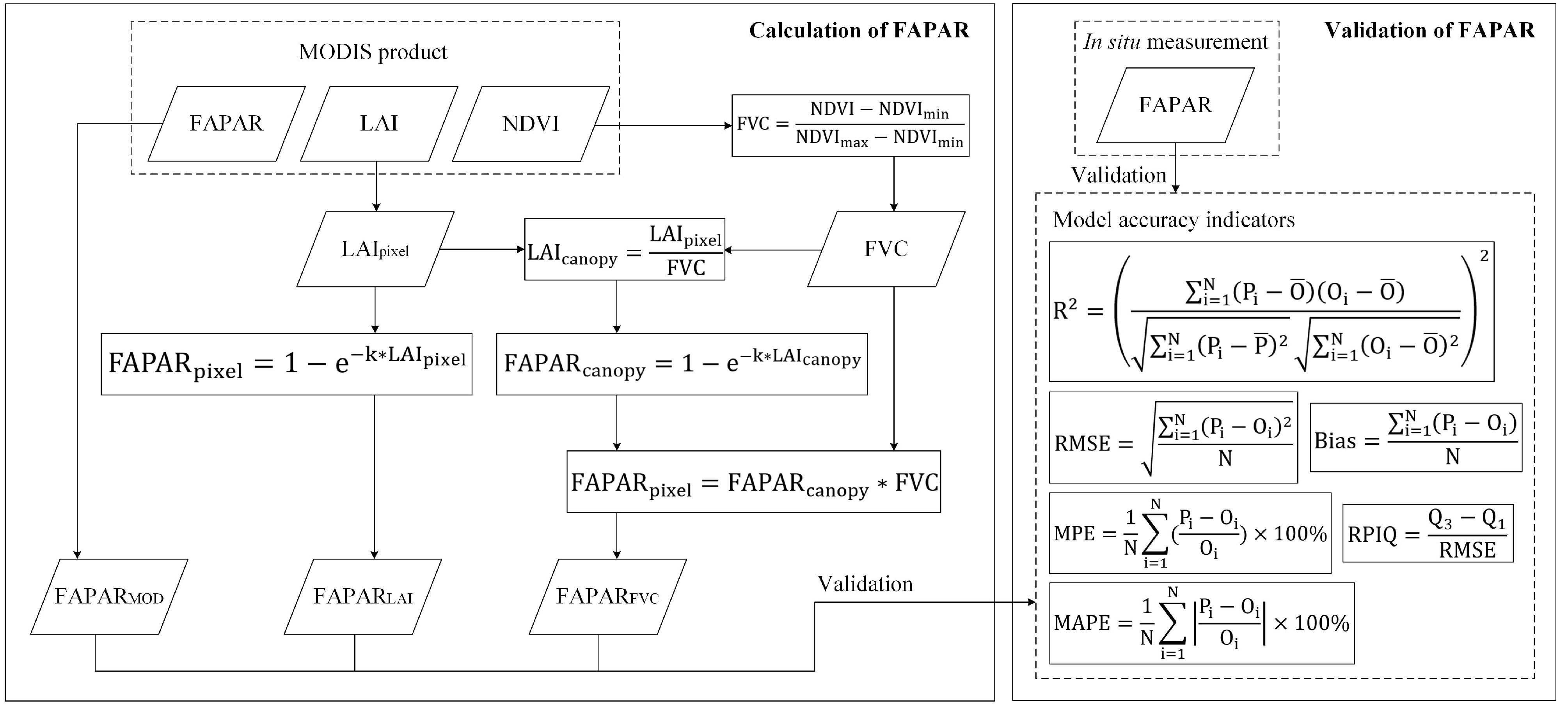
The fundamental premise of the Beer-Lambert’s law, which forms the basis of the calculation of FAPAR based on LAI, is the assumption of a homogeneous turbid medium vegetation canopy [39,40,41]. However, for vegetation types such as summer-green vegetation, canopy distributions tend to exhibit clear phenological variations, with the green leaves of the plants concentrated only in areas with green canopy distribution. Therefore, the proportion of the green canopy distribution area can be determined based on the FVC, and then the average LAI of the pixel (sample site) (LAI_pixel) can be converted into the LAI of the actual green canopy distribution area (LAI_canopy) based on the FVC, and then calculate the FAPAR of the green canopy distribution area (FAPAR_canopy) to reduce the influence of heterogeneity on the estimation of FAPAR caused by the distribution of non-green canopies, and finally derive the average FAPAR of the pixel (sample site) (FAPAR_pixel) based on the FVC (Figure 1). The schematic flowchart of the presented FAPAR models was shown in Figure 2.

2.2.2. Calculation of FAPAR

For a pixel (sample site), its FAPAR can be considered as the average of FAPAR within the pixel (sample site), encompassing both the green canopy distribution area and the non-green canopy distribution area. This can be calculated based on the canopy-scale FAPAR within the green canopy distribution area and the FVC in the pixel (sample site):

$${\mathrm{F}\mathrm{A}\mathrm{P}\mathrm{A}\mathrm{R}}_{\mathrm{p}\mathrm{i}\mathrm{x}\mathrm{e}\mathrm{l}}={\mathrm{F}\mathrm{A}\mathrm{P}\mathrm{A}\mathrm{R}}_{\mathrm{c}\mathrm{a}\mathrm{n}\mathrm{o}\mathrm{p}\mathrm{y}}\ast \mathrm{F}\mathrm{V}\mathrm{C}$$

(2)

where FAPAR_pixel is the FAPAR at the pixel (sample site) scale, FAPAR_canopy is the canopy-scale FAPAR of the green vegetation canopy distribution area, FVC is the fractional vegetation coverage, and FAPAR_canopy in the green canopy distribution area can be expressed as:

$${\mathrm{F}\mathrm{A}\mathrm{P}\mathrm{A}\mathrm{R}}_{\mathrm{c}\mathrm{a}\mathrm{n}\mathrm{o}\mathrm{p}\mathrm{y}}=1-{\mathrm{e}}^{-\mathrm{k}\ast {\mathrm{L}\mathrm{A}\mathrm{I}}_{\mathrm{c}\mathrm{a}\mathrm{n}\mathrm{o}\mathrm{p}\mathrm{y}}}$$

(3)

where k is the extinction coefficient, set at 0.5 [14,15], and LAI_canopy is the leaf area index of the green canopy distribution area.

For LAI measured at the pixel (sample site) scale, it should reflect the average situation of LAI for that pixel (sample site), which can be defined as LAI_pixel. This can be regarded as the products of the canopy-scale LAI_canopy within the green vegetation canopy distribution area and FVC, thus expressed as:

$${\mathrm{L}\mathrm{A}\mathrm{I}}_{\mathrm{p}\mathrm{i}\mathrm{x}\mathrm{e}\mathrm{l}}={\mathrm{L}\mathrm{A}\mathrm{I}}_{\mathrm{c}\mathrm{a}\mathrm{n}\mathrm{o}\mathrm{p}\mathrm{y}}\ast \mathrm{F}\mathrm{V}\mathrm{C}$$

(4)

Consequently, LAI_canopy can be calculated based on the pixel (sample site) scale LAI_pixel and FVC:

$${\mathrm{L}\mathrm{A}\mathrm{I}}_{\mathrm{c}\mathrm{a}\mathrm{n}\mathrm{o}\mathrm{p}\mathrm{y}}={\displaystyle \frac{{\mathrm{L}\mathrm{A}\mathrm{I}}_{\mathrm{p}\mathrm{i}\mathrm{x}\mathrm{e}\mathrm{l}}}{\mathrm{F}\mathrm{V}\mathrm{C}}}$$

(5)

LAI_pixel can be derived from MODIS LAI, and FVC can be inferred from MODIS NDVI as discussed in Section 2.2.1.

2.2.3. Validation of FAPAR

In this study, the coefficient of determination (R²), root mean squared error (RMSE), and mean prediction error (Bias) were employed to evaluate the estimation accuracy of FAPAR:

$${\mathrm{R}}^2={\left({\displaystyle \frac{{\sum }_{\mathrm{i}=1}^{\mathrm{N}}\left({\mathrm{P}}_{\mathrm{i}}-\overline{\mathrm{O}}\right)\left({\mathrm{O}}_{\mathrm{i}}-\overline{\mathrm{O}}\right)}{\sqrt{{\sum }_{\mathrm{i}=1}^{\mathrm{N}}{\left({\mathrm{P}}_{\mathrm{i}}-\overline{\mathrm{P}}\right)}^2}\sqrt{{\sum }_{\mathrm{i}=1}^{\mathrm{N}}{\left({\mathrm{O}}_{\mathrm{i}}-\overline{\mathrm{O}}\right)}^2}}}\right)}^2$$

(6)

$$\mathrm{R}\mathrm{M}\mathrm{S}\mathrm{E}=\sqrt{{\displaystyle \frac{{\sum }_{\mathrm{i}=1}^{\mathrm{N}}{\left({\mathrm{P}}_{\mathrm{i}}-{\mathrm{O}}_{\mathrm{i}}\right)}^2}{\mathrm{N}}}}$$

(7)

$$\mathrm{B}\mathrm{i}\mathrm{a}\mathrm{s}={\displaystyle \frac{{\sum }_{\mathrm{i}=1}^{\mathrm{N}}\left({\mathrm{P}}_{\mathrm{i}}-{\mathrm{O}}_{\mathrm{i}}\right)}{\mathrm{N}}}$$

(8)

where P_i, O_i, $\overline{\mathrm{O}}$ represent the predicted, observed, and mean of the observed values of the samples, respectively, and N signifies the number of samples. Given the observation that FAPAR exhibited significant variation across different biome types and that the impact of lower FAPAR biome types might be underestimated when solely RMSE and Bias are utilized for assessment, the mean absolute percentage error (MAPE) and the mean percentage error (MPE), and the ratio of performance to interquartile range (RPIQ) were also evaluated [50,51].

$$\mathrm{M}\mathrm{A}\mathrm{P}\mathrm{E}={\displaystyle \frac{1}{\mathrm{N}}}\sum _{\mathrm{i}=1}^{\mathrm{N}}\left|{\displaystyle \frac{{\mathrm{P}}_{\mathrm{i}}-{\mathrm{O}}_{\mathrm{i}}}{{\mathrm{O}}_{\mathrm{i}}}}\right|\times 100\%$$

(9)

$$\mathrm{M}\mathrm{P}\mathrm{E}={\displaystyle \frac{1}{\mathrm{N}}}\sum _{\mathrm{i}=1}^{\mathrm{N}}\left({\displaystyle \frac{{\mathrm{P}}_{\mathrm{i}}-{\mathrm{O}}_{\mathrm{i}}}{{\mathrm{O}}_{\mathrm{i}}}}\right)\times 100\%$$

(10)

$$\mathrm{R}\mathrm{P}\mathrm{I}\mathrm{Q}={\displaystyle \frac{{\mathrm{Q}}_3-{\mathrm{Q}}_1}{\mathrm{R}\mathrm{M}\mathrm{S}\mathrm{E}}}$$

(11)

where Q₁ is the value below which we can find 25% of the samples; Q₃ is the value below which we find 75% of the samples. This paper evaluates the MODIS FPAR products, the FAPAR calculated using Beer-Lambert’s law based on the MODIS LAI products, and the improved FAPAR that uses Beer-Lambert’s law by considering FVC. The three FAPARs are abbreviated as FAPAR_MOD, FAPAR_LAI, and FAPAR_FVC, respectively.

3. Results

3.1. Overall Situation of Model Accuracy

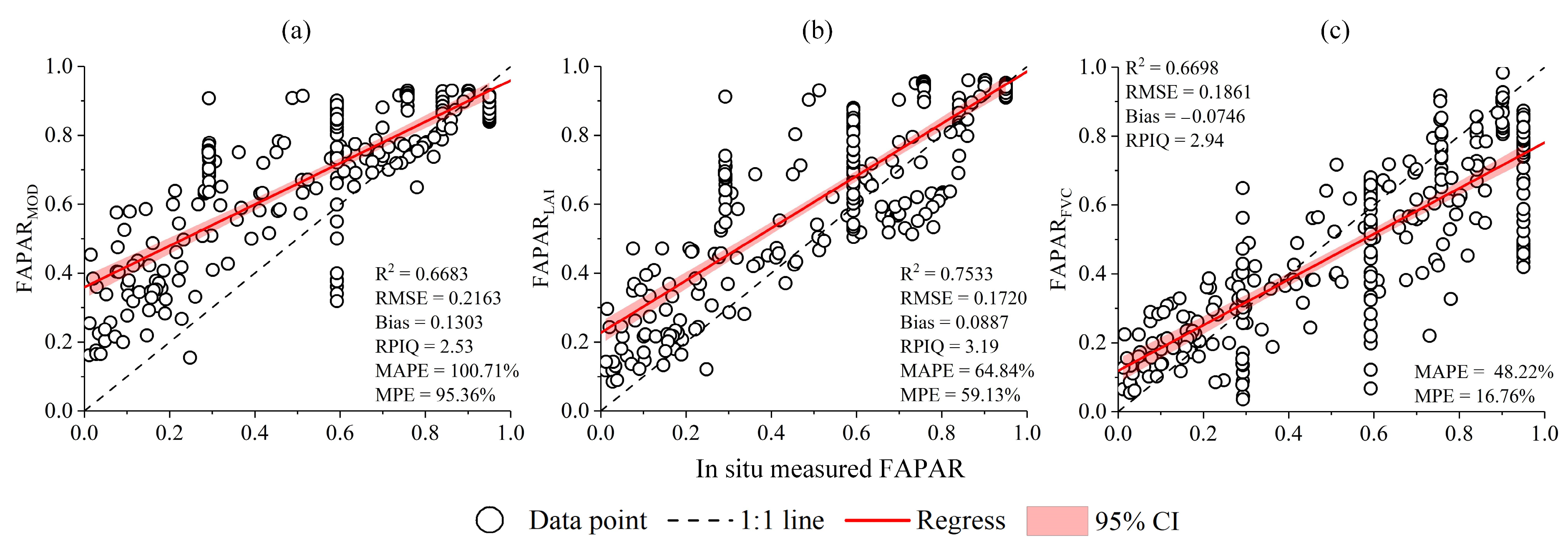
The accuracy of FAPAR_MOD was clearly lower than that of comparison models. The RMSE and MAPE of FAPAR_MOD were 0.216 and 100.7%, respectively, while the RMSE of FAPAR_LAI and FAPAR_FVC were 0.172 and 0.186, respectively, which were reduced by 20.5% and 13.9%, respectively; the MAPE were 64.8% and 48.2%, which were reduced by 35.6% and 52.1%, respectively; the RPIQ was 2.53, while that of FAPAR_LAI and FAPAR_FVC were 3.19 and 2.94, which were 26.1% and 16.2% higher, respectively. The Bias and MPE of FAPAR_MOD were 0.130 and 95.4%, respectively, while the Bias of FAPAR_LAI and FAPAR_FVC were 0.089 and −0.075, respectively, which were 31.9% and 42.8% lower in terms of quantity (regardless of positivity and negativity); the MPE were 59.1% and 16.8%, which were 38.0% and 82.4% lower in terms of quantity, respectively. The R² of FAPAR_MOD was 0.668, and the R² of FAPAR_LAI and FAPAR_FVC were 0.753 and 0.670, which were 12.7% and 0.3% higher, respectively (Figure 3).

The accuracy of FAPAR_FVC is clearly superior to that of FAPAR_LAI. The MAPE and MPE are notably better, with MAPE and MPE of 48.2% and 16.8%, respectively, for FAPAR_FVC, compared to 64.8% and 59.1%, respectively, for FAPAR_LAI, which is a reduction of 25.6% and 71.6%, respectively. RMSE, Bias, RPIQ, and R² were generally similar, with FAPAR_FVC having an 8.2% higher RMSE, a 7.8% lower RPIQ, and a 11.0% lower R² compared to FAPAR_LAI, but a 15% lower Bias, in terms of quantity, respectively (Figure 3).

All three models simulate FAPAR as overestimated, with FAPAR_FVC being the least overestimated. The MPE of FAPAR_MOD, FAPAR_LAI, and FAPAR_FVC are 95.4%, 59.1%, and 16.8%, respectively, and the MPE of FAPAR_MOD and FAPAR_LAI are 5.7 and 3.7 times the MPE of FAPAR_FVC, respectively. However, FAPAR_FVC exhibits an underestimation with a Bias of −0.075 (Figure 3).

3.2. Differences in Model Accuracy Between Biome Types

Most of the biome types showed an overestimation of FAPAR_MOD. Grass savanna, desert, arctic tundra, tallgrass prairie, cropland, temperate needleleaf forest, and temperate mixed forest showed an overestimation of FAPAR_MOD, and boreal forest and tropical broadleaf evergreen forest showed underestimation. The overestimated biomes ranged from 0.088 to 0.280 for Bias and 25.1% to 350.1% for MPE. Boreal forest and tropical broadleaf evergreen forest had Bias of −0.012 and −0.066, respectively, and MPE of −1.9% and −6.9%. Among overestimated biomes, cropland and grass savanna had the most prominent overestimation of FAPAR_MOD with MPE of 350.1% and 333.8%, respectively. This was followed by arctic tundra and desert with MPE of 168.3% and 111.2%, respectively. Then came the temperate mixed forest and tallgrass prairie, with MPE of 41.3% and 72.9% for the two sites in temperate mixed forest and 50.6% for tallgrass prairie. The least overestimated was the temperate needleleaf forest with an MPE of 25.1% (Figure 4 and

Table 2. The accuracies for FAPAR estimation in different biome types. FAPAR was the same in Figure 1. FAPAR_MOD, FAPAR_LAI, FAPAR_FVC, FVC, R², RMSE, Bias, RPIQ, MAPE, and MPE were the same in Figure 2. For biome types overestimated by FAPAR_MOD, FAPAR_LAI and FAPAR_FVC estimated FAPAR with clearly lower overestimates compared to FAPAR_MOD, with FAPAR_FVC being more clearly lower. For the biome types underestimated by FAPAR_MOD, the underestimation of FAPAR was more severe for FAPAR_LAI and FAPAR_FVC, especially for FAPAR_FVC.

Vegetation Type	Site Name	Model	R2	RMSE	Bias	RPIQ	MAPE (%)	MPE (%)
grass savanna	Dahra + Tessekre	FAPARMOD	0.90	0.20	0.18	1.92	333.75	333.75
		FAPARLAI	0.91	0.13	0.11	2.88	195.71	195.38
		FAPARFVC	0.94	0.10	0.08	3.85	142.72	141.36
arctic tundra	TUND	FAPARMOD	0.23	0.30	0.28	0.68	168.30	168.30
		FAPARLAI	0.02	0.19	0.14	1.07	109.16	107.56
		FAPARFVC	0.61	0.10	0.05	2.10	50.52	45.24
cropland (corn and soybean)	AGRO	FAPARMOD	0.87	0.25	0.20	1.86	350.12	350.12
		FAPARLAI	0.89	0.16	0.04	3.01	217.02	203.62
		FAPARFVC	0.93	0.13	−0.01	3.64	154.70	134.37
temperate mixed forest	CHEQ	FAPARMOD	0.75	0.22	0.19	1.97	43.99	41.30
		FAPARLAI	0.83	0.21	0.19	2.08	39.97	36.32
		FAPARFVC	0.84	0.10	0.03	4.55	19.19	4.36
	HARV	FAPARMOD	0.76	0.31	0.23	1.96	73.19	72.91
		FAPARLAI	0.79	0.27	0.21	2.22	65.05	64.50
		FAPARFVC	0.78	0.16	−0.06	3.90	30.16	−10.31
tallgrass prairie	KONZ	FAPARMOD	0.78	0.16	0.09	2.12	52.61	50.64
		FAPARLAI	0.83	0.15	−0.07	2.27	38.69	9.07
		FAPARFVC	0.79	0.19	−0.14	1.80	37.43	−9.67
boreal forest	NOBS	FAPARMOD	0.71	0.10	−0.01	0.20	8.53	−1.92
		FAPARLAI	0.36	0.10	−0.04	0.20	8.88	−4.65
		FAPARFVC	0.47	0.21	−0.15	0.10	19.31	−19.10
desert	SEVI	FAPARMOD	0.48	0.16	0.16	0.21	111.18	111.18
		FAPARLAI	0.42	0.05	0.04	0.66	34.01	31.16
		FAPARFVC	0.59	0.04	0.03	0.84	24.16	19.66
tropical broadleaf evergreen forest	TAPA	FAPARMOD	-	0.07	−0.07	-	6.91	−6.91
		FAPARLAI	-	0.02	−0.02	-	1.86	−1.85
		FAPARFVC	-	0.32	−0.28	-	29.48	−29.48
temperate needleleaf forest	METL	FAPARMOD	-	0.23	0.15	-	37.75	25.10
		FAPARLAI	-	0.18	0.15	-	27.28	25.43
		FAPARFVC	-	0.18	−0.09	-	22.17	−14.99

).

For biome types overestimated by FAPAR_MOD, FAPAR_LAI and FAPAR_FVC estimated FAPAR with clearly lower overestimates compared to FAPAR_MOD, with FAPAR_FVC being more clearly lower. The MAPE of FAPAR_LAI varied from 27.3 to 217.0%, with an average reduction of 32.3% compared to FAPAR_MOD; the MPE varied from 9.1 to 203.6%, with an average reduction of 37.0% compared to FAPAR_MOD; and the RPIQ of FAPAR_LAI varied from 0.20 to 3.01, with an average increase of 31.4% compared to FAPAR_MOD. The MAPE of FAPAR_FVC varied from 19.2 to 154.7%, with an average reduction of 55.8% compared to FAPAR_MOD; the MPE varied from −15.0 to 141.4%, with an average reduction of 71.4% in terms of quantity compared to FAPAR_MOD; and the RPIQ of FAPAR_FVC varied from 0.10 to 4.55, with an average increase of 89.8% compared to FAPAR_MOD (Figure 4 and Table 2).

For the biome types underestimated by FAPAR_MOD, the underestimation of FAPAR was more severe for FAPAR_LAI and FAPAR_FVC, especially for FAPAR_FVC. The MPE of FAPAR_LAI for boreal forest was −4.7%, which is 141.9% higher in terms of quantity compared to FAPAR_MOD, but the underestimation of FAPAR_LAI for tropical broadleaf evergreen forest was improved, with an MPE of −1.85%, which is 73.2% lower in terms of quantity compared to FAPAR_MOD. The underestimation of FAPAR_FVC was more severe in both boreal forest and tropical broadleaf evergreen forest, with an MPE of −19.1% and −29.5%, respectively, which were 894.8% and 326.9% lower compared to FAPAR_MOD (Figure 4 and Table 2).

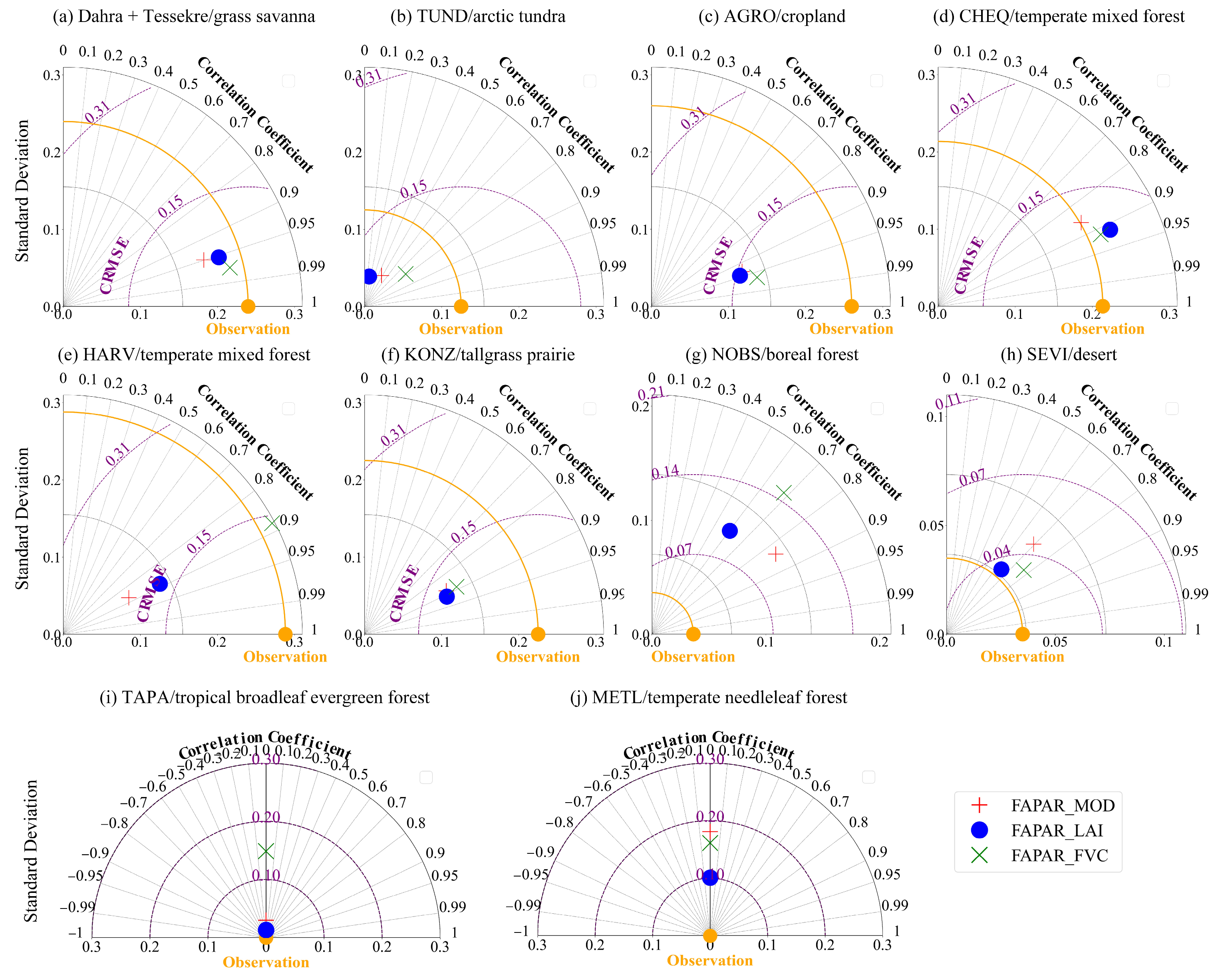
To visually evaluate the comprehensive accuracy of the three FAPAR models in terms of SD (Standard deviation), R (Correlation coefficient), and CRMSE (Centered root mean squared error) across various biome types [52], Taylor diagrams were generated using the SM module from the sklearn.metrics library in Python [53]. FAPAR_FVC exhibited superior comprehensive accuracy in grass savanna, arctic tundra, cropland, temperate mixed forest, tallgrass prairie, and desert ecosystems. In contrast, FAPAR_LAI showed better integrated performance in tropical broadleaf evergreen forest and temperate needleleaf forest environments and FAPAR_MOD achieved optimal accuracy in boreal forest regions (Figure 5).

3.3. Differences in Model Accuracy in Temporal Changes

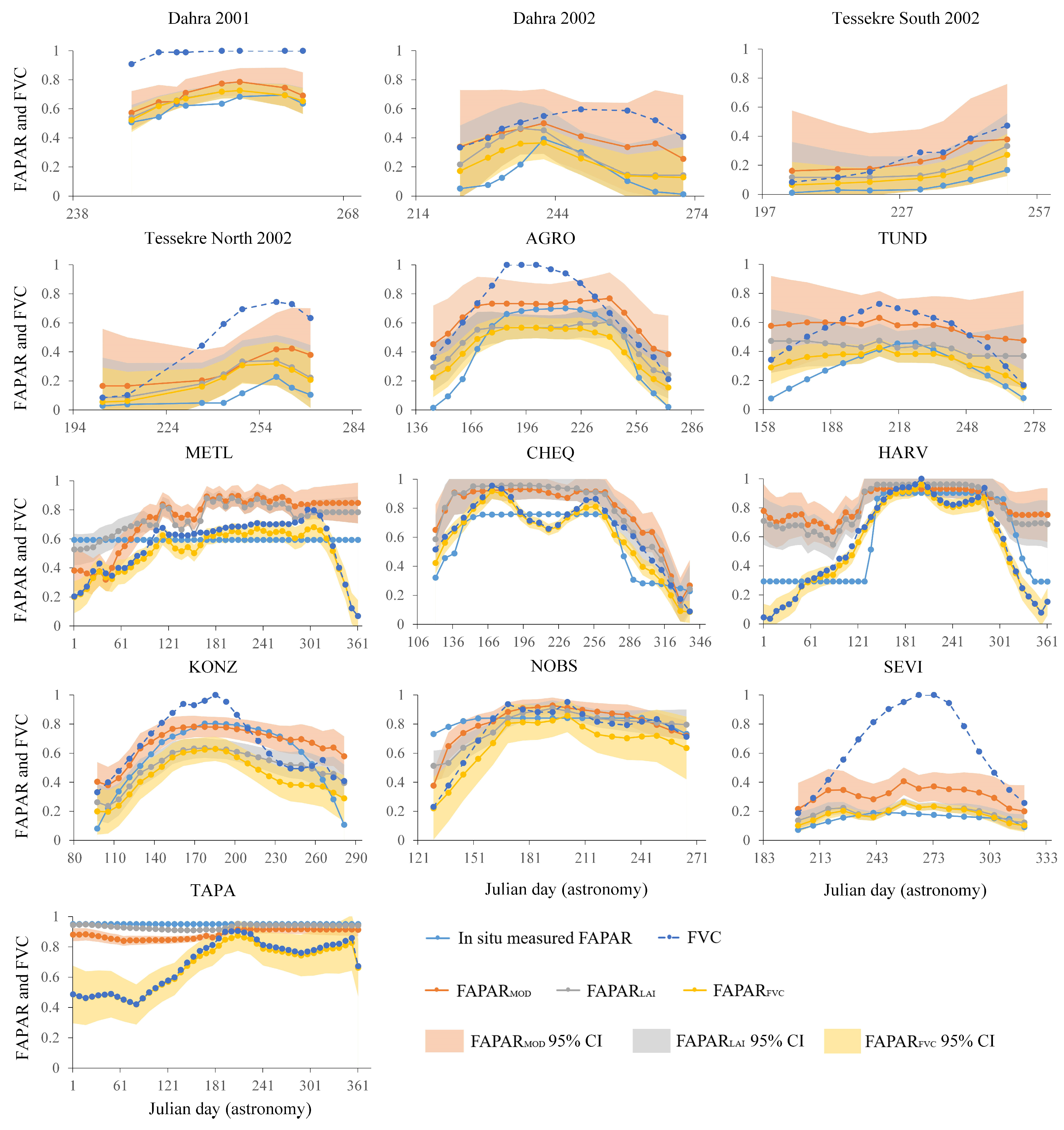
With the exception of the tropical evergreen broadleaf forest, the vegetation in the other biome types exhibited distinct phenological changes (Figure 6). Alongside the intra-annual variation of vegetation, most biome types (grass savanna, cropland, arctic tundra, temperate mixed forest, tallgrass prairie, and desert) demonstrated overestimation of FAPAR by each model during the off-peak vegetation growth period. The overestimation by FAPAR_MOD was more obvious, followed by FAPAR_LAI and FAPAR_FVC. At the peak of the vegetation growth period, all FAPAR models showed a reduction in overestimation, with some biome types (cropland and tallgrass prairie) beginning to be underestimated (Figure 6).

The Dahra data from the grass savanna represented two years of observational data (2001 and 2002) collected at the same site. The improvement in the presented method over the two years exhibited a consistent pattern. Despite the notable disparity in FAPAR between 2001 and 2002, the accuracy of FAPAR_FVC was clearly higher than that of FAPAR_LAI and FAPAR_MOD in both years. Specifically, the MAPE decreased by 9.1% and 50.2% in 2001, and by 18.9% and 56.7% in 2002, respectively.

The accuracies of the estimated FAPAR during the peak vegetation growth period were higher than those during the off-peak vegetation growth period. The MAPE and MPE of FAPAR_MOD were 171.9% and 165.8% during the off-peak vegetation growth period, respectively, while those over the peak growth period were 34.3% and 29.7%, respectively. The former were 5.0 and 5.6 times higher than those for the latter. The MAPE and MPE of FAPAR_LAI were 110.6% and 106.2% during the off-peak vegetation growth period, respectively, compared to 22.1% and 15.3% for the peak vegetation growth period, with the former being 5.0 and 6.9 times higher than the latter. The MAPE and MPE of FAPAR_FVC were 76.1% and 42.2% during the off-peak vegetation growth period, respectively, compared to 22.2% and −7.0% for the peak growth period, with the former being 3.4 and 6.0 times more in terms of quantity than the latter (

Table 3. Comparison for estimated FAPAR accuracies between different vegetation growth periods. FAPAR, FAPAR_MOD, FAPAR_LAI, FAPAR_FVC, FVC, RMSE, Bias, MAPE, and MPE were the same in Figure 2. FAPAR_FVC showed clearly higher improvement in the overestimation of FAPAR compared to FAPAR_LAI and FAPAR_MOD during the off-peak growth period than during the peak growth period.

Model	Vegetation Growth Stage	RMSE	Bias	MAPE (%)	MPE (%)
FAPARMOD	off-peak growth period	0.274	0.201	171.9	165.8
	peak growth period	0.142	0.065	34.3	29.7
FAPARLAI	off-peak growth period	0.216	0.149	110.6	106.2
	peak growth period	0.117	0.032	22.2	15.3
FAPARFVC	off-peak growth period	0.173	−0.038	76.1	42.2
	peak growth period	0.197	−0.108	22.2	−7.0

).

For FAPAR_LAI and FAPAR_FVC compared to FAPAR_MOD, FAPAR_FVC showed clearly higher improvement in the overestimation of FAPAR during the off-peak growth period than during the peak growth period, whereas FAPAR_LAI showed a similar improvement over both periods. FAPAR_FVC reduced MAPE by 35.3% and 55.7% and MPE by 74.5% and 95.8% over both periods, respectively, while FAPAR_LAI reduced MAPE by 35.7% and 35.3% and MPE by 35.0% and 38.6% over both periods, respectively (Table 3 and Figure 6).

Compared to FAPAR_LAI, the improvements in accuracy and decrease in overestimation for FAPAR_FVC were clearer during the off-peak vegetation growth period than during the peak vegetation growth period; the accuracy of FAPAR_FVC did not change much during the peak vegetation growth period, but the overestimation condition was reduced clearly. MAPE and MPE were 110.6% and 103.2% for FAPAR_LAI, and 76.1% and 42.2% for FAPAR_FVC during the off-peak growth period, which were reduced by 31.1% and 60.2%, respectively. During the peak vegetation growth period, MAPE was 22.2% for both FAPAR_LAI and FAPAR_FVC, but MPE was 15.3% and −7.0%, respectively, a 54.4% decrease in terms of quantity.

3.4. Model Accuracy and Fractional Vegetation Coverage

The accuracy of all three models in simulating FAPAR increased with increasing FVC. FAPAR_MOD had a MAPE of 19.4%, 131.55%, and 255.6%, and an MPE of 16.8%, 125.2%, and 244.9% for high, medium, and low FVC, respectively. FAPAR_LAI had a MAPE of 14.0%, 83.4%, and 164.4%, and an MPE of 7.6%, 78.4%, and 158.2% under high, medium, and low FVC, respectively. FAPAR_FVC had a MAPE of 14.0%, 65.4%, and 97.9%, and an MPE of −4.1%, 33.1%, and 25.4% under high, medium, and low FVC, respectively (

Table 4. Difference in FAPAR estimation accuracies with different FVC ranges. FAPAR was the same in Figure 1. FAPAR_MOD, FAPAR_LAI, FAPAR_FVC, FVC, RMSE, Bias, MAPE, and MPE were the same in Figure 2. The accuracy of all three models in simulating FAPAR increased with increasing FVC.

FAPAR	FVC Range	RMSE	Bias	MAPE (%)	MPE (%)
FAPARMOD	70–90%	0.124	0.068	19.4	16.8
	30–70%	0.247	0.162	131.5	125.2
	0–30%	0.314	0.221	255.8	244.9
FAPARLAI	70–90%	0.113	0.036	14.0	7.6
	30–70%	0.189	0.112	83.4	78.4
	0–30%	0.248	0.177	164.4	158.2
FAPARFVC	70–90%	0.115	−0.056	14.0	−4.1
	30–70%	0.223	−0.077	65.4	33.1
	0–30%	0.221	−0.129	97.9	25.4

).

Compared to FAPAR_MOD, FAPAR_LAI and FAPAR_FVC generally showed a decrease in the improvement of FAPAR accuracy with increasing FVC. The proportion of FAPAR decrease gradually increased with decreasing FVC (Figure 7a). The actual statistics of FAPAR_FVC reduction compared to FAPAR_LAI in this paper also showed a gradual increase with decreasing FVC (Figure 7b). FAPAR_LAI decreased MAPE by 27.6%, 36.6%, and 35.7% under high, medium, and low FVC, but MPE decreased by 54.6%, 37.3%, and 35.4%, respectively. FAPAR_FVC reduced MAPE by 27.7%, 50.3%, and 60.3% and MPE by 75.4%, 73.5%, and 89.6% under high, medium, and low FVC conditions, respectively (Table 4).

Compared to FAPAR_LAI, the improvement in accuracy for FAPAR_FVC was clearer with decreasing FVC. The MAPE of FAPAR_LAI were 14.0%, 83.4%, and 164.4%, respectively, and the FAPAR_FVC were 14.0%, 65.4%, and 97.9%, respectively, which were reduced by 0.2%, 21.5%, and 67.9%, respectively, under high, medium, and low FVC conditions; the MPE of FAPAR_LAI were 7.6%, 78.4%, and 158.2%, respectively, and the FAPAR_FVC were −4.1%, 33.1%, and 25.4%, respectively, which were reduced by 45.9%, 79.1%, and 83.9% in terms of quantity, respectively (Table 4). For the FAPAR_MOD overestimated biome types, the average FVC was 60.7 ± 24.4%, whereas for the biome types underestimated at FAPAR_MOD, the FVC was 72.3 ± 17.9% (

Table 5. Average FVC of different biome types. FAPAR was the same in Figure 1. FAPAR_MOD and FVC were the same in Figure 2.

FAPARMOD	Biome Types	Site Name	N	Average FVC	Standard Deviation
Overestimation	arctic tundra	TUND	15	0.523	0.163
	temperate needleleaf forest	METL	46	0.557	0.186
	temperate mixed forest	HARV	46	0.559	0.320
	grass savanna	Dahra + Tessekre	32	0.564	0.304
	desert	SEVI	16	0.639	0.285
	temperate mixed forest	CHEQ	28	0.657	0.221
	tallgrass prairie	KONZ	24	0.665	0.210
	cropland (corn and soybean)	AGRO	17	0.696	0.260
Underestimation	tropical broadleaf evergreen forest	TAPA	46	0.689	0.164
	boreal forest	NOBS	18	0.757	0.193

).

3.5. Relationship Between FAPAR Error and LAI Error

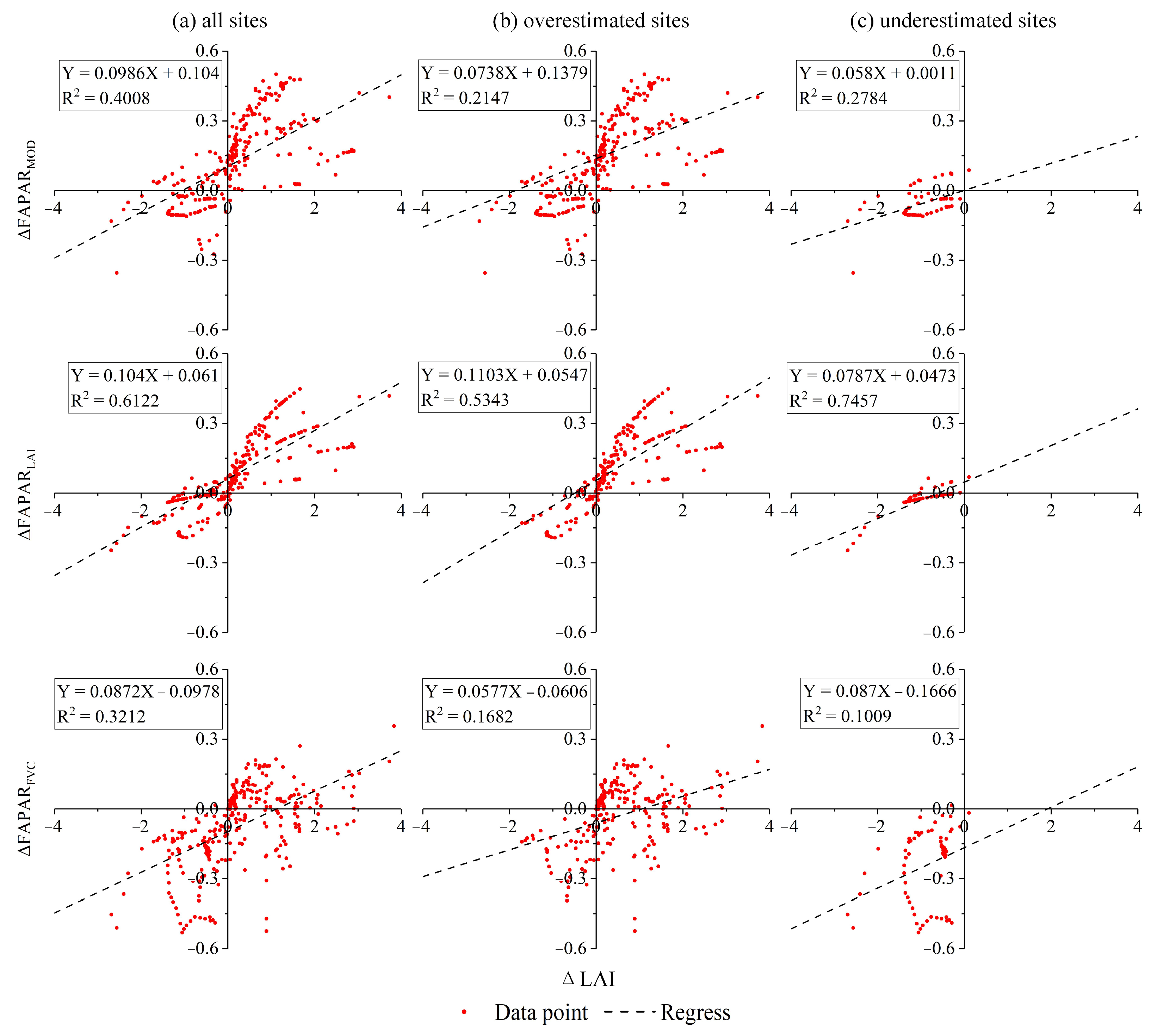
There was a significant correlation between LAI error (difference between MODIS LAI and in situ measured LAI) and FAPAR error (difference between estimated FAPAR and in situ measured FAPAR). From all samples, LAI error was significantly positively associated with errors from FAPAR_MOD, FAPAR_LAI, and FAPAR_FVC, and the R² of the regression equations were 0.401, 0.612, and 0.321, respectively (N = 288, p < 0.001). For the samples at biome types with overestimated FAPAR_MOD, the R² of the regression equations of LAI errors with errors from FAPAR_MOD, FAPAR_LAI, and FAPAR_FVC were 0.215, 0.534, and 0.168 (N = 224, p < 0.001), respectively. For the samples at biome types with underestimated FAPAR_MOD, the R² of the regression equations of LAI errors and errors from FAPAR_MOD, FAPAR_LAI, and FAPAR_FVC were 0.278 (N = 64, p < 0.001), 0.746 (N = 64, p < 0.001), and 0.101 (N = 64, p = 0.011), respectively (Figure 8).

From the full data, the LAI error explained 61.2% of the variation in FAPAR_LAI error and a 32.1% for the FAPAR_FVC error. For the samples at biome types with FAPAR_MOD overestimated, the LAI error explained 53.4% of the variation in FAPAR_LAI error and 16.8% for the FAPAR_FVC error. For the samples at sites with FAPAR_MOD underestimated, the LAI error explained 74.6% of the variation in the FAPAR_LAI error and 10.1% for FAPAR_FVC error. For the three groups of samples, after considering the FVC, the ability of LAI error to explain the variation in the FAPAR error was reduced by 47.5%, 68.5%, and 86.5%, respectively, basically more than 50% (Figure 8).

4. Discussion

4.1. Impact of Fractional Vegetation Coverage Estimation Errors on FAPAR_MOD

In this paper, we demonstrate that although the same set of MODIS LAI data is used to calculate FAPAR, the accuracy of FAPAR_LAI is clearly better than FAPAR_MOD, and the accuracy of FAPAR_FVC is clearly better than FAPAR_LAI. FAPAR_MOD calculates FAPAR based on the stochastic radiative transfer (SRT) model [54,55,56]. The SRT-based model was particularly improved for heterogeneous vegetation canopies, considering a mechanism of streaming radiation through canopy gaps; the detailed radiative transfer process of light through the canopy was taken into account in calculating FAPAR; the differences in parameters of different vegetation types were taken into account. However, errors in the estimation of FVC may have led to errors in the estimation of FAPAR_MOD due to the lack of an accurate model of the FVC [40].

There is a large intra-annual variation in the FVC of the green part of the canopy in summer-green vegetation such as grasslands, shrubs, and forests, or in vegetation that is clearly influenced by the wet and dry seasons. The green FVC is low during the off-peak vegetation growth period and may be clearly lower than the range of FVC given in the MODIS algorithm, and it may be only during the peak growth period that the FVC is roughly in line with the range given in the MODIS algorithm [7,57]. Thus, at times other than the peak growth period, the FVC may be clearly lower than the range given in the MODIS algorithm [58].

The overestimation of FVC in the MODIS algorithm actually exaggerates the distribution area of the green vegetation canopy, that is, it is equivalent to spreading the green leaves of the vegetation more dispersed inside the pixel (sample site) (Figure 1). As the green leaves are more evenly spread within the pixel, the shading effect between the leaves is reduced, and thus may lead to an overestimation of the absorption of solar radiation from the vegetation by the green leaves, resulting in an overestimation of the FAPAR.

The results of this paper showed that FAPAR_MOD exhibited overestimation for all biome types except for tropical broadleaf evergreen forest and boreal forest during the growth period, and that the overestimation of FAPAR_MOD was more pronounced during the off-peak growth period within the growth period (Figure 6), which may be related to the fact that MODIS algorithms for these vegetation types overestimated FVC during the off-peak growth period. Other studies have also shown that FAPAR_MOD overestimation occurs during the off-peak vegetation growth period [20,21,22,23,24], suggesting that the overestimation of FVC by the MODIS algorithm during these periods may have contributed to the overestimation of FAPAR_MOD.

In addition to the errors arising from FVC due to the MODIS FVC model, the misclassification of land cover type in MODIS pixels and the presence of heterogeneous land cover types with low LAI due to the presence of snow, water bodies, etc., can also affect the accuracy of the FVC estimation in calculating the estimation of the FAPAR. A study in the Mongo area of Zambia concluded that misclassifying the vegetation type at this observation site as savanna led to an incorrect estimation of the FVC, which ultimately resulted in an overestimation of FAPAR [7]. In the polar tundra of Alaska, the overestimation of FAPAR in the early and late growth period may be related to snow cover on the ground [59,60].

4.2. Effect of Presence in Non-Green Vegetation Canopy on FAPAR Estimation

FAPAR_LAI uses the Beer-Lambert’s law, a simple form of radiative transfer, to calculate FAPAR directly, whereas FAPAR_MOD calculates FAPAR based on the more complex stochastic radiative transfer (SRT) model [54,55,56]. However, both FAPAR calculations are based on the Beer-Lambert’s law. Since the vegetation canopy in most biome types cannot satisfy the homogeneous turbid medium assumption of Beer-Lambert’s law at the pixel (sample site) scale, and the presence of non-green vegetation canopies also causes errors in FAPAR_MOD and FAPAR_LAI, and FAPAR_FVC obtains a more accurate FAPAR by introducing a more accurate model of the FVC.

For cases where there is clear phenological variation in the vegetation canopy or where non-vegetation canopy is present, green leaves are concentrated in areas where green canopy is distributed. Because the Beer-Lambert’s law uses a homogeneous turbid medium assumption, green leaves are also assumed to be distributed in non-green canopy distribution areas, potentially underestimating the shading effect between leaves, which in turn exaggerates the absorption of solar radiation by vegetation, leading to an overestimation of FAPAR. Compared to the FAPAR_LAI, under different LAI conditions, FAPAR_FVC gradually decreased with decreasing FVC (Figure 7).

As a result, the improvement magnitude in FAPAR_FVC accuracy increased with the decrease in FVC compared to FAPAR_LAI (Table 4). For the FAPAR_MOD overestimated biome types, the average FVC was clearly lower than the biome types underestimated at FAPAR_MOD (Table 5), and thus the FAPAR overestimation was more clearly corrected by the FAPAR for the biome types with lower FVC (Figure 3). For most biome types, due to the obvious phenological changes in vegetation, both FAPAR_MOD and FAPAR_LAI showed overestimation as vegetation entered the growth period; with the gradual increase in the FVC, the GPP overestimation gradually decreased, during the peak vegetation growth period FAPAR overestimation eased, and then after the peak period GPP overestimation increased with the decrease in FVC (Figure 6). Since FAPAR_FVC takes into account the effect of FVC, relative to FAPAR_LAI, FAPAR accuracy improved and overestimation reduced over the off-peak vegetation growth period, and accuracy did not change much over the peak vegetation growth period (Table 3).

For boreal forest and tropical broadleaf evergreen forest, the increased underestimation of FAPAR_FVC is mainly related to the already existing underestimation of FAPAR_LAI. With FAPAR_LAI itself underestimated, FAPAR_FVC will be less than FAPAR_LAI after accounting for the effect of FVC, thus increasing the underestimation of FAPAR.

4.3. Impact of MODIS LAI Errors on FAPAR Estimation

Although the accuracy of FAPAR_FVC has been clearly better than that of FAPAR_LAI, it still has clear errors and the errors are still dominated by overestimation (Figure 3), which suggests that there are other factors affecting the accuracy of FAPAR in addition to the FVC. Since FAPAR_MOD, FAPAR_LAI and FAPAR_FVC are all calculated based on the MODIS LAI products based on the Beer-Lambert’s law, the estimated FAPAR error may be related to the LAI error. The observation in this study indicated there was a significant correlation between LAI error (difference between MODIS LAI and in situ measured LAI) and FAPAR error (difference between estimated FAPAR and in situ measured FAPAR).

From all samples, the samples at biome types with FAPAR_MOD overestimated and the samples at biome types with FAPAR_MOD underestimated, LAI error was all significantly positively associated with errors from FAPAR_MOD (Figure 8). Therefore, in addition to the factor of FVC affecting the estimated FAPAR accuracy, the accuracy of the MODIS LAI products used also have an important effect. For the three groups of samples, after considering the FVC, the ability of LAI error to explain variation in FAPAR error was reduced by basically more than 50% (Figure 8). Considering that there may be other factors which affect FAPAR accuracy, the reduction in FAPAR estimation error by considering the FVC may be roughly comparable or higher than the LAI-induced error (Figure 8).

The overestimation and underestimation of FAPAR_FVC are primarily associated with errors in MODIS LAI. As shown in Figure 8, the underestimation samples are derived from tropical broadleaf evergreen forests and boreal forests, where MODIS LAI is consistently underestimated across all samples. This underestimation of LAI consequently led to the underestimation of FAPAR in these sites. Conversely, at other sites where overestimation occurs, the number of samples with overestimated LAI clearly exceeds those with underestimated LAI, resulting in an overestimation of FAPAR.

4.4. Research Uncertainties and Future Studies

Uncertainty was first brought by NDVI data. In this paper, the FVC is introduced to improve the simulation of FAPAR, and the FVC calculation is obtained based on the NDVI calculated from remote sensing data. As the remote sensing data are affected by clouds and rain, it may lead to the underestimation of NDVI, and the underestimation of NDVI will lead to the underestimation of FVC, which in turn will lead to the underestimation of FAPAR_FVC. From the NDVI extracted from the tropical rainforest, the distribution of NDVI is about 0.4 from January to April, and 0.7 to 0.8 in other months in 2004. In the tropical rainforest area, the vegetation grows luxuriantly all year-round, and the lower NDVI may be the result of more rainfall during the corresponding period of this site [61,62,63]. The lower NDVI induced by clouds and rain may lead to the underestimation of FVC, which further leads to the underestimation of FAPAR_FVC. Therefore, the increased underestimation of FAPAR in the tropical rainforest region may also be related to the lower NDVI induced by clouds.

The NDVI is used to calculate FVC; however, NDVI may reach saturation, particularly in tropical regions with high FVC, where the NDVI typically saturates at an average value of approximately 0.8 [64]. Under this condition, both LAI and FAPAR are also at relatively high levels, and FVC is also at a high level, nearly approaching 100%. This means that NDVI saturation should not affect the FVC estimation greatly. In addition, as illustrated in Figure 7, when FVC is high, its influence on the calculation of the FAPAR_FVC model is relatively minor. When NDVI approaches saturation, FVC itself is already high. Thus, even if NDVI saturation induces some uncertainties in FVC estimation, its effect on the FAPAR_FVC should be limited. However, under conditions of low FVC, NDVI may be influenced by soil background effects. Vegetation indices that are less affected by soil background, such as EVI and SAVI, could be considered for estimating FVC.

Another uncertainty in FAPAR accuracy evaluation arises from the reliability of ground-based FAPAR measurements. The in situ measurements of FAPAR from the BigFoot project and three grassland in situ measured sites in Senegal, West Africa, were converted based on LAI data using Beer-Lambert’s law [43], which assumes that leaves are opaque and does not take into account reflections from the soil and canopy. Therefore, the Beer-Lambert’s law calculation should yield the interception PAR [7,65,66]. Considering that leaves are opaque and that there is absorption of solar radiation by non-green parts, the in situ measured FAPAR absorbed by green leaves should be overestimated. Reducing the interception of solar radiation by excluding soil and canopy reflectance would underestimate the FAPAR absorbed by green leaves, but the underestimation would only be 1% on average [7]. The fraction of interception PAR absorbed by leaves varies widely among plants, generally from 0.75 to 0.90 [67,68,69,70,71], implying that soil and canopy reflectance have a relatively small effect on the measurement of FAPAR absorbed by green leaves. Thus, the overestimation of FAPAR absorbed by green leaves due to leaf opacity and the presence of non-green portions is likely to be more pronounced. Because of the possible overestimation of FAPAR as validation data, the degree of overestimation of FAPAR_MOD, FAPAR_LAI, and FAPAR_FVC may be slightly higher than those in this study.

The non-homogeneous turbid canopy of forests or shrubs may also influence the results. Although introducing FVC can partially solve the problem of non-green vegetation canopy, this method essentially assumes that the distribution of leaves of each individual tree or shrub can be approximated as satisfying the homogeneous turbid medium assumption. Thus, this assumption is still not fully applicable in the complex vegetation structures of forests or shrubs since they exhibit three-dimensional features. The current methodology is unable to address this limitation, and further in-depth research is required to improve upon this shortcoming.

The results of this paper show that the accuracy of FAPAR_LAI calculated based on MODIS LAI is better than that of FAPAR_MOD, and FAPAR_FVC considering the effect of FVC is clearly better than FAPAR_LAI. This FAPAR algorithm can also be used for regional-scale GPP estimation, thus obtaining more accurate GPP and providing more reliable data for the analysis of GPP tempo-spatial patterns and its drivers [72]. However, the results also showed that even though the accuracy of FAPAR_FVC with FVC taken into account was clearly improved, a systematic overestimation still persisted, and the main source of error may be related to the error of MODIS LAI data, especially in biomes with significant underestimation of LAI, such as tropical broadleaf evergreen forest and boreal forest. Therefore, it is necessary to pay more attention to reducing the error of MODIS LAI and obtaining more accurate NDVI data in the subsequent GPP estimation.

5. Conclusions

This paper proposes a method to improve FAPAR estimation based on the Beer-Lambert’s law considering FVC, and conducts a case study using FAPAR and LAI from the BigFoot Project as well as from field measurements of grass savanna in Senegal, West Africa, and corresponding MODIS products. The results show that the accuracy in FAPAR_FVC is clearly better than those based on FAPAR_LAI as well as FAPAR_MOD, and FAPAR_LAI accuracy is also clearly better than FAPAR_MOD. The improvements in accuracy and the decrease in overestimation for FAPAR_FVC were clearer with decreasing FVC compared to FAPAR_LAI. The results indicate that the FAPAR_FVC method can improve the accuracy of FAPAR estimation under the presence of non-green vegetation canopies. The method can be extended to regional FAPAR and GPP simulations, providing more accurate inputs for understanding their tempo-spatial patterns and its drivers. Although the FAPAR_FVC method can improve FAPAR estimation, there is still a systematic overestimation which may be related to the error of MODIS LAI data, and thus more in-depth study is required to reduce the error of MODIS LAI.

References

1. Sabzchi-Dehkharghani, H.; Biswas, A.; Meshram, S.G.; Majnooni-Heris, A. Estimating gross and net primary productivities using earth observation products: A review. Environ. Model. Assess. 2024, 29, 179–200. [Google Scholar] [CrossRef]
2. Pei, Y.Y.; Dong, J.W.; Zhang, Y.; Yuan, W.P.; Doughty, R.; Yang, J.L.; Zhou, D.C.; Zhang, L.X.; Xiao, X.M. Evolution of light use efficiency models: Improvement, uncertainties, and implications. Agric. For. Meteorol. 2022, 317, 108905. [Google Scholar] [CrossRef]
3. Hilker, T.; Coops, N.C.; Wulder, M.A.; Black, T.A.; Guy, R.D. The use of remote sensing in light use efficiency based models of gross primary production: A review of current status and future requirements. Sci. Total Environ. 2008, 404, 411–423. [Google Scholar] [CrossRef] [PubMed]
4. Li, Z.H.; Zhang, Q.; Li, J.; Yang, X.; Wu, Y.F.; Zhang, Z.Y.; Wang, S.H.; Wang, H.Z.; Zhang, Y.G. Solar-induced chlorophyll fluorescence and its link to canopy photosynthesis in maize from continuous ground measurements. Remote Sens. Environ. 2020, 236, 111420. [Google Scholar] [CrossRef]
5. Goward, S.N.; Huemmrich, K.F. Vegetation canopy PAR absorptance and the normalized difference vegetation index: An assessment using the SAIL model. Remote Sens. Environ. 1992, 39, 119–140. [Google Scholar] [CrossRef]
6. Hipps, L.E.; Asrar, G.; Kanemasu, E.T. Assessing the interception of photosynthetically active radiation in winter wheat. Agric. Meteorol. 1983, 28, 253–259. [Google Scholar] [CrossRef]
7. Huemmrich, K.F.; Privette, J.L.; Mukelabai, M.; Myneni, R.B.; Knyazikhin, Y. Time-series validation of MODIS land biophysical products in a Kalahari woodland, Africa. Int. J. Remote Sens. 2005, 26, 4381–4398. [Google Scholar] [CrossRef]
8. Yan, G.J.; Hu, R.H.; Luo, J.H.; Weiss, M.; Jiang, H.L.; Mu, X.H.; Xie, D.H.; Zhang, W.M. Review of indirect optical measurements of leaf area index: Recent advances, challenges, and perspectives. Agric. For. Meteorol. 2019, 265, 390–411. [Google Scholar] [CrossRef]
9. Xiao, X.; Hollinger, D.; Aber, J.; Goltz, M.; Davidson, E.A.; Zhang, Q.; Moore, B., III. Satellite-based modeling of gross primary production in an evergreen needleleaf forest. Remote Sens. Environ. 2004, 89, 519–534. [Google Scholar] [CrossRef]
10. Xiao, X.; Zhang, Q.; Braswell, B.; Urbanski, S.; Boles, S.; Wofsy, S.; Moore, B., III; Ojima, D. Modeling gross primary production of temperate deciduous broadleaf forest using satellite images and climate data. Remote Sens. Environ. 2004, 91, 256–270. [Google Scholar] [CrossRef]
11. Sims, D.A.; Rahman, A.F.; Cordova, V.D.; Baldocchi, D.D.; Flanagan, L.B.; Goldstein, A.H.; Hollinger, D.Y.; Misson, L.; Monson, R.K.; Schmid, H.P.; et al. Midday values of gross CO2 flux and light use efficiency during satellite overpasses can be used to directly estimate eight-day mean flux. Agric. For. Meteorol. 2005, 131, 1–12. [Google Scholar] [CrossRef]
12. Yuan, W.; Liu, S.; Zhou, G.; Zhou, G.; Tieszen, L.L.; Baldocchi, D.; Bernhofer, C.; Gholz, H.; Goldstein, A.H.; Goulden, M.L.; et al. Deriving a light use efficiency model from eddy covariance flux data for predicting daily gross primary production across biomes. Agric. For. Meteorol. 2007, 143, 189–207. [Google Scholar] [CrossRef]
13. He, M.; Ju, W.; Zhou, Y.; Chen, J.; He, H.; Wang, S.; Wang, H.; Guan, D.; Yan, J.; Li, Y.; et al. Development of a two-leaf light use efficiency model for improving the calculation of terrestrial gross primary productivity. Agric. For. Meteorol. 2013, 173, 28–39. [Google Scholar] [CrossRef]
14. Guan, X.B.; Chen, J.M.; Shen, H.F.; Xie, X.Y. A modified two-leaf light use efficiency model for improving the simulation of GPP using a radiation scalar. Agric. For. Meteorol. 2021, 307, 108546. [Google Scholar] [CrossRef]
15. Guan, X.B.; Chen, J.M.; Shen, H.F.; Xie, X.Y.; Tan, J.B. Comparison of big-leaf and two-leaf light use efficiency models for GPP simulation after considering a radiation scalar. Agric. For. Meteorol. 2022, 313, 108761. [Google Scholar] [CrossRef]
16. Sun, Y.K.; Yuan, D.K.; Zheng, X.; Yang, S.S.; Zhang, S.; Zhang, J.H.; Bai, Y. Estimation of radiation scalar using deep learning for improved gross primary productivity estimation based on a light-use efficiency model. Int. J. Digit. Earth 2024, 17, 2402421. [Google Scholar] [CrossRef]
17. Huang, L.X.; Yuan, W.P.; Zheng, Y.; Zhou, Y.L.; He, M.Z.; Jin, J.X.; Huang, X.J.; Chen, S.Y.; Liu, M.; Guan, X.B.; et al. A dynamic-leaf light use efficiency model for improving gross primary production estimation. Environ. Res. Lett. 2024, 19, 014066. [Google Scholar] [CrossRef]
18. Verhoef, W. Light-scattering by leaf layers with application to canopy reflectance modeling—The SAIL model. Remote Sens. Environ. 1984, 16, 125–141. [Google Scholar] [CrossRef]
19. Jacquemoud, S.; Baret, F.; Andrieu, B.; Danson, F.M.; Jaggard, K. Extraction of vegetation biophysical parameters by inversion of the PROSPECT + SAIL models on sugar beet canopy reflectance data. Application to TM and AVIRIS sensors. Remote Sens. Environ. 1995, 52, 163–172. [Google Scholar] [CrossRef]
20. Fensholt, R.; Sandholt, I.; Rasmussen, M.S. Evaluation of MODIS LAI, fAPAR and the relation between fAPAR and NDVI in a semi-arid environment using in situ measurements. Remote Sens. Environ. 2004, 91, 490–507. [Google Scholar] [CrossRef]
21. Steinberg, D.C.; Goetz, S.J.; Hyer, E.J. Validation of MODIS FPAR products in boreal forests of Alaska. IEEE Trans. Geosci. Remote. Sens. 2006, 44, 1818–1828. [Google Scholar] [CrossRef]
22. D’Odorico, P.; Gonsamo, A.; Pinty, B.; Gobron, N.; Coops, N.; Mendez, E.; Schaepman, M.E. Intercomparison of fraction of absorbed photosynthetically active radiation products derived from satellite data over Europe. Remote Sens. Environ. 2014, 142, 141–154. [Google Scholar] [CrossRef]
23. Chernetskiy, M.; Gómez-Dans, J.; Gobron, N.; Morgan, O.; Lewis, P.; Truckenbrodt, S.; Schmullius, C. Estimation of FAPAR over croplands using MISR data and the earth observation land data assimilation system (EO-LDAS). Remote Sens. 2017, 9, 656. [Google Scholar] [CrossRef]
24. Stocker, B.D.; Wang, H.; Smith, N.G.; Harrison, S.P.; Keenan, T.F.; Sandoval, D.; Davis, T.; Prentice, I.C. P-model v1.0: An optimality-based light use efficiency model for simulating ecosystem gross primary production. Geosci. Model Dev. 2020, 13, 1545–1581. [Google Scholar] [CrossRef]
25. Zheng, Y.J.; Xiao, Z.Q.; Li, J.; Yang, H.; Song, J.L. Evaluation of global fraction of absorbed photosynthetically active radiation (FAPAR) products at 500 m spatial resolution. Remote Sens. 2022, 14, 3304. [Google Scholar] [CrossRef]
26. Lai, P.Y.; Marshall, M.; Darvishzadeh, R.; Nelson, A. Crop productivity under heat stress: A structural analysis of light use efficiency models. Agric. For. Meteorol. 2025, 362, 110376. [Google Scholar] [CrossRef]
27. Liang, S.Z.; Hou, X.H.; Sui, X.Y.; Wang, M. Deciduous broadleaf forests green FPAR and its relationship with spectral vegetation indices. In Proceedings of the 2017 10th International Congress on Image and Signal Processing, BioMedical Engineering and Informatics (CISP-BMEI), Shanghai, China, 14–16 October 2017; pp. 1–5. [Google Scholar] [CrossRef]
28. Majasalmi, T.; Stenberg, P.; Rautiainen, M. Comparison of ground and satellite-based methods for estimating stand-level fPAR in a boreal forest. Agric. For. Meteorol. 2017, 232, 422–432. [Google Scholar] [CrossRef]
29. Tan, C.W.; Wang, D.L.; Zhou, J.; Du, Y.; Luo, M.; Zhang, Y.J.; Guo, W.S. Remotely assessing fraction of photosynthetically active radiation (FPAR) for wheat canopies based on hyperspectral vegetation indexes. Front. Plant Sci. 2018, 9, 776. [Google Scholar] [CrossRef] [PubMed]
30. Zhang, Y.; Li, S.H.; He, Z.; Liu, Y.H.; Su, Z.H. Synergistic inversion of rice FPAR based on optical and radar remote sensing data. In Proceedings of the IGARSS 2019—2019 IEEE International Geoscience and Remote Sensing Symposium, Yokohama, Japan, 28 July–2 August 2019; pp. 1943–1946. [Google Scholar] [CrossRef]
31. Haboudane, D.; Miller, J.R.; Pattey, E.; Zarco-Tejada, P.J.; Strachan, I.B. Hyperspectral vegetation indices and novel algorithms for predicting green LAI of crop canopies: Modeling and validation in the context of precision agriculture. Remote Sens. Environ. 2004, 90, 337–352. [Google Scholar] [CrossRef]
32. Huete, A.R. A soil-adjusted vegetation index (SAVI). Remote Sens. Environ. 1988, 25, 295–309. [Google Scholar] [CrossRef]
33. Frederic, B.; Guyot, G.; Major, D. TSAVI: A vegetation index which minimizes soil brightness effects on LAI and APAR estimation. In Proceedings of the 12th Canadian Symposium on Remote Sensing Geoscience and Remote Sensing Symposium, Vancouver, BC, Canada, 10–14 July 1989; pp. 1355–1358. [Google Scholar] [CrossRef]
34. Qi, J.; Chehbouni, A.; Huete, A.R.; Kerr, Y.H.; Sorooshian, S. A modified soil adjusted vegetation index. Remote Sens. Environ. 1994, 48, 119–126. [Google Scholar] [CrossRef]
35. Ruimy, A.; Kergoat, L.; Bondeau, A. Comparing global models of terrestrial net primary productivity (NPP): Analysis of differences in light absorption and light-use efficiency. Glob. Change Biol. 1999, 5, 56–64. [Google Scholar] [CrossRef]
36. Zhang, Y.H.; Hu, Z.W.; Fang, H.L.; Gao, X.; Wang, J.Z.; Wu, G.F. Estimation of daily FAPAR from MODIS instantaneous observations at forest sites. Agric. For. Meteorol. 2023, 331, 109336. [Google Scholar] [CrossRef]
37. Xiao, Z.; Liang, S.; Wang, T.; Jiang, B. Retrieval of leaf area index (LAI) and fraction of absorbed photosynthetically active radiation (FAPAR) from VIIRS time-series data. Remote Sens. 2016, 8, 351. [Google Scholar] [CrossRef]
38. Zhu, H.; Lin, A.; Wang, L.; Xia, Y.; Zou, L. Evaluation of MODIS gross primary production across multiple biomes in China using eddy covariance flux data. Remote Sens. 2016, 8, 395. [Google Scholar] [CrossRef]
39. Florakis, K.; Trevezas, S.; Letort, V. Predicting tomato water consumption in a hydroponic greenhouse: Contribution of light interception models. Front. Plant Sci. 2023, 14, 1264915. [Google Scholar] [CrossRef] [PubMed]
40. Shabanov, N.; Gastellu-Etchegorry, J.-P. The stochastic Beer–Lambert–Bouguer law for discontinuous vegetation canopies. J. Quant. Spectrosc. Radiat. Transf. 2018, 214, 18–32. [Google Scholar] [CrossRef]
41. Ponce de León, M.A.; Bailey, B.N. Evaluating the use of Beer’s law for estimating light interception in canopy architectures with varying heterogeneity and anisotropy. Ecol. Model. 2019, 406, 133–143. [Google Scholar] [CrossRef]
42. Nilson, T. A theoretical analysis of the frequency of gaps in plant stands. Agric. Meteorol. 1971, 8, 25–38. [Google Scholar] [CrossRef]
43. Turner, D.P.; Ritts, W.D.; Gregory, M. BigFoot GPP and NPP summary, 2000–2004. 2006. Available online: https://daac.ornl.gov/BIGFOOT_VAL/gpp_npp_summaries.html (accessed on 16 October 2024).
44. Goulden, M.L.; Daube, B.C.; Fan, S.-M.; Sutton, D.J.; Bazzaz, A.; Munger, J.W.; Wofsy, S.C. Physiological responses of a black spruce forest to weather. J. Geophys. Res. Atmos. 1997, 102, 28987–28996. [Google Scholar] [CrossRef]
45. Meyers, T.P.; Hollinger, S.E. An assessment of storage terms in the surface energy balance of maize and soybean. Agric. For. Meteorol. 2004, 125, 105–115. [Google Scholar] [CrossRef]
46. Wofsy, S.C.; Goulden, M.L.; Munger, J.W.; Fan, S.M.; Bakwin, P.S.; Daube, B.C.; Bassow, S.L.; Bazzaz, F.A. Net exchange of CO2 in a mid-latitude forest. Science 1993, 260, 1314–1317. [Google Scholar] [CrossRef]
47. Kurc, S.A.; Small, E.E. Dynamics of evapotranspiration in semiarid grassland and shrubland ecosystems during the summer monsoon season, central New Mexico. Water Resour. Res. 2004, 40, W09305. [Google Scholar] [CrossRef]
48. Anthoni, P.M.; Unsworth, M.H.; Law, B.E.; Irvine, J.R.; Baldocchi, D.D.; Tuyl, S.V.; Moore, D. Seasonal differences in carbon and water vapor exchange in young and old-growth ponderosa pine ecosystems. Agric. For. Meteorol. 2002, 111, 203–222. [Google Scholar] [CrossRef]
49. Savitzky, A.; Golay, M.J.E. Smoothing and differentiation of data by simplified least squares procedures. Anal. Chem. 1964, 36, 1627–1639. [Google Scholar] [CrossRef]
50. Jiang, Z.Y.; Huete, A.R.; Chen, J.; Chen, Y.H.; Li, J.; Yan, G.J.; Zhang, X.Y. Analysis of NDVI and scaled difference vegetation index retrievals of vegetation fraction. Remote Sens. Environ. 2006, 101, 366–378. [Google Scholar] [CrossRef]
51. Gutman, G.; Ignatov, A. The derivation of the green vegetation fraction from NOAA/AVHRR data for use in numerical weather prediction models. Int. J. Remote Sens. 1998, 19, 1533–1543. [Google Scholar] [CrossRef]
52. Taylor, K.E. Summarizing multiple aspects of model performance in a single diagram. J. Geophys. Res. Atmos. 2001, 106, 7183–7192. [Google Scholar] [CrossRef]
53. Rochford, P.A. SkillMetrics: A Python Package for Calculating the Skill of Model Predictions Against Observations. 2016. Available online: http://github.com/PeterRochford/SkillMetrics (accessed on 29 January 2025).
54. Shabanov, N.V.; Knyazikhin, Y.; Baret, F.; Myneni, R.B. Stochastic Modeling of Radiation Regime in Discontinuous Vegetation Canopies. Remote Sens. Environ. 2000, 74, 125–144. [Google Scholar] [CrossRef]
55. Shabanov, N.V.; Huang, D.; Knjazikhin, Y.; Dickinson, R.E.; Myneni, R.B. Stochastic radiative transfer model for mixture of discontinuous vegetation canopies. J. Quant. Spectrosc. Radiat. Transf. 2007, 107, 236–262. [Google Scholar] [CrossRef]
56. Huang, D.; Knyazikhin, Y.; Wang, W.; Deering, D.W.; Stenberg, P.; Shabanov, N.; Tan, B.; Myneni, R.B. Stochastic transport theory for investigating the three-dimensional canopy structure from space measurements. Remote Sens. Environ. 2008, 112, 35–50. [Google Scholar] [CrossRef]
57. Kanniah, K.D.; Beringer, J.; Hutley, L.B.; Tapper, N.J.; Zhu, X. Evaluation of Collections 4 and 5 of the MODIS Gross Primary Productivity product and algorithm improvement at a tropical savanna site in northern Australia. Remote Sens. Environ. 2009, 113, 1808–1822. [Google Scholar] [CrossRef]
58. Knyazikhin, Y.; Martonchik, J.V.; Myneni, R.B.; Diner, D.J.; Running, S.W. Synergistic algorithm for estimating vegetation canopy leaf area index and fraction of absorbed photosynthetically active radiation from MODIS and MISR data. J. Geophys. Res. Atmos. 1998, 103, 32257–32275. [Google Scholar] [CrossRef]
59. Turner, D.P.; Ritts, W.D.; Cohen, W.B.; Maeirsperger, T.K.; Gower, S.T.; Kirschbaum, A.A.; Running, S.W.; Zhao, M.S.; Wofsy, S.C.; Dunn, A.L.; et al. Site-level evaluation of satellite-based global terrestrial gross primary production and net primary production monitoring. Glob. Change Biol. 2005, 11, 666–684. [Google Scholar] [CrossRef]
60. Turner, D.P.; Ritts, W.D.; Zhao, M.S.; Kurc, S.A.; Dunn, A.L.; Wofsy, S.C.; Small, E.E.; Running, S.W. Assessing interannual variation in MODIS-based estimates of gross primary production. IEEE Trans. Geosci. Remote Sens. 2006, 44, 1899–1907. [Google Scholar] [CrossRef]
61. Chen, B.Q.; Li, X.P.; Xiao, X.M.; Zhao, B.; Dong, J.W.; Kou, W.L.; Qin, Y.W.; Yang, C.; Wu, Z.X.; Sun, R.; et al. Mapping tropical forests and deciduous rubber plantations in Hainan Island, China by integrating PALSAR 25-m and multi-temporal Landsat images. Int. J. Appl. Earth Obs. Geoinf. 2016, 50, 117–130. [Google Scholar] [CrossRef]
62. Gao, S.P.; Liu, X.L.; Bo, Y.C.; Shi, Z.T.; Zhou, H.M. Rubber identification based on blended high spatio-temporal resolution optical remote sensing data: A case study in Xishuangbanna. Remote Sens. 2019, 11, 496. [Google Scholar] [CrossRef]
63. Jiao, J.N.; Shi, J.; Tian, Q.J.; Gao, L.; Xu, N.X. Research on multispectral-image-based NDVI shadow-effect-eliminating model. Natl. Remote Sens. Bull. 2020, 24, 53–66. [Google Scholar] [CrossRef]
64. Knyazikhin, Y.; Glassy, J.; Privette, J.L.; Tian, Y.; Lotsch, A.; Zhang, Y.; Wang, Y.; Morisette, J.T.; Votava, P.; Myneni, R.B.; et al. MODIS Leaf Area Index (LAI) and Fraction of Photosynthetically Active Radiation Absorbed by Vegetation (FPAR) Product (MOD15) Algorithm Theoretical Basis Document. 1999. Available online: https://modis.gsfc.nasa.gov/data/atbd/atbd_mod15.pdf (accessed on 29 January 2025).
65. Huemmrich, K.F.; Goward, S.N. Vegetation canopy PAR absorptance and NDVI: An assessment for ten tree species with the SAIL model. Remote Sens. Environ. 1997, 61, 254–269. [Google Scholar] [CrossRef]
66. Huemmrich, K.F. The GeoSail model: A simple addition to the SAIL model to describe discontinuous canopy reflectance. Remote Sens. Environ. 2001, 75, 423–431. [Google Scholar] [CrossRef]
67. Ehleringer, J. Leaf absorptances of mohave and sonoran desert plants. Oecologia 1981, 49, 366–370. [Google Scholar] [CrossRef]
68. Krall, J.P.; Edwards, G.E. Relationship between photosystem-II activity and CO2 fixation in leaves. Physiol. Plant. 1992, 86, 180–187. [Google Scholar] [CrossRef]
69. Björkman, O.; Demmig, B. Photon yield of O2 evolution and chlorophyll fluorescence characteristics at 77 K among vascular plants of diverse origins. Planta 1987, 170, 489–504. [Google Scholar] [CrossRef]
70. He, L.; He, X.P.; Bian, J.M.; Zhu, C.L.; Fu, J.R.; Wu, Y.; He, H.H. Application of mechanistic model of light-response of photosynthetic electron flow on photosynthetic characteristics in super late rice. J. South. Agric. 2019, 50, 1937–1944. [Google Scholar]
71. Ye, Z.P.; Hu, W.H.; Yan, X.H.; Fan, D.Y.; Yin, J.H.; Duan, S.H.; Yan, X.H.; He, L.; Zhang, S.S. A mechanistic model of light-response of photosynthetic electron flow and its application. Chin. J. Plant Ecol. 2014, 38, 1241–1249. [Google Scholar] [CrossRef]
72. Zheng, Y.Y.; Zhao, W.Q.; Chen, A.P.; Chen, Y.; Chen, J.N.; Zhu, Z.C. Vegetation canopy structure mediates the response of gross primary production to environmental drivers across multiple temporal scales. Sci. Total Environ. 2024, 917, 170439. [Google Scholar] [CrossRef]
Figure 1. The conceptual models of the fraction of absorbed photosynthetically active radiation (FAPAR) for green vegetation canopy (FAPARcanopy) and FAPAR for a pixel (sample site) (FAPARpixel). (a) Actual distribution of vegetation green canopy within pixels, where subpixels with green leaves present are green canopy distribution areas; (b) Average green canopy conditions at the pixel (sample site) scale under the Beer-Lambert’s law assumption, with green leaves evenly distributed in each subpixel. LAIcanopy is the amount of leaf area per unit of horizontal ground surface with green leaves present in Figure 1a and FAPARcanopy is the absorbed PAR by green leaves in the same area; LAIpixel is the mean of leaf area per unit of horizontal ground surface within the whole pixel in Figure 1a and FAPARpixel is the average of absorbed PAR by green leaves in the same area. FVC is the fractional vegetation coverage. The relationship between LAIpixel and LAIcanopy can be expressed as LAIpixel = LAIcanopy * FVC.
Remotesensing 17 00603 g001
Figure 2. The schematic flowchart of the presented FAPAR model. FAPAR, FAPARpixel, FAPARcanopy, LAIpixel, LAIcanopy, and FVC were the same in Figure 1. NDVI: normalized difference vegetation index; NDVImax and NDVImin: the 95th and the 5th percentile of NDVI over the growth period within the study area, respectively; R2: coefficient of determination; RMSE: root mean squared error; Bias: mean prediction error; MAPE: mean absolute percentage error; MPE: mean percentage error; RPIQ: ratio of performance to interquartile range.
Remotesensing 17 00603 g002
Figure 3. The accuracies in FAPAR estimation for FAPARMOD, FAPARLAI, and FAPARFVC: (a) the accuracy of FAPARMOD; (b) the accuracy of FAPARLAI; (c) the accuracy of FAPARFVC. FAPARMOD, FAPARLAI, and FAPARFVC are FAPAR from MODIS FPAR products, FAPAR calculated using Beer-Lambert’s law based on the MODIS LAI products, and the improved FAPAR that uses Beer-Lambert’s law by considering FVC, respectively. FAPAR, FAPARMOD, FAPARLAI, FAPARFVC, FVC, R2, RMSE, Bias, RPIQ, MAPE, and MPE were the same in Figure 2. CI refers to the confidence interval. The accuracy of FAPARLAI is higher than that of FAPARMOD, and the accuracy of FAPARFVC is superior to that of FAPARLAI.
Remotesensing 17 00603 g003
Figure 4. The accuracies for FAPAR estimation in different biome types. FAPAR was the same in Figure 1. FAPARMOD, FAPARLAI, FAPARFVC, FVC, R2, RMSE, Bias, RPIQ, MAPE, MPE, and CI were the same in Figure 3. For biome types overestimated by FAPARMOD, FAPARLAI and FAPARFVC estimated FAPAR with clearly lower overestimates compared to FAPARMOD, with FAPARFVC being more clearly lower. For the biome types underestimated by FAPARMOD, the underestimation of FAPAR was more severe for FAPARLAI and FAPARFVC, especially for FAPARFVC.
Remotesensing 17 00603 g004
Figure 5. Taylor diagrams of three FAPAR models across various biome types. The black concentric circles denote the standard deviation (SD); the angular position corresponds to the correlation coefficient (R). The purple concentric circles indicate the centered root mean squared error (CRMSE). Additionally, the yellow marker (labeled “Observation”) shows the position of observational data’s SD, R, and CRMSE values, while the yellow arc highlights simulated results sharing equivalent SD with the observational data. FAPARMOD, FAPARLAI, and FAPARFVC were the same in Figure 2.
Remotesensing 17 00603 g005
Figure 6. Intra-annual variation in FAPAR estimation for different biome types. FAPAR was the same in Figure 1. FAPARMOD, FAPARLAI, FAPARFVC, and FVC were the same in Figure 2. Most biome types demonstrated overestimation of FAPAR by each model during the off-peak vegetation growth period.
Remotesensing 17 00603 g006
Figure 7. Scatterplot of fractional vegetation coverage versus FAPAR reduction calculated by taking fractional vegetation coverage into account: (a) FAPAR reduction from different assumed LAI after considering fractional vegetation coverage; (b) FAPAR reduction from the data used in this study after considering fractional vegetation coverage. Change rate = (FAPARLAI − FAPARFVC)/FAPARLAI, with the extinction coefficient set to 0.5 when calculating FAPAR using the Beer-Lambert’s law. FAPAR was the same in Figure 1. FAPARLAI, FAPARFVC, and FVC were the same in Figure 2. The proportion of FAPAR decrease gradually increased with decreasing FVC.
Remotesensing 17 00603 g007
Figure 8. Scatterplot of MODIS LAI error versus errors for FAPARMOD, FAPARLAI, and FAPARFVC: (a) All data; (b) Samples in biome types with FAPARMOD overestimated; (c) Samples in biome types with FAPARMOD underestimated. Y-axis represents the estimated FAPAR error, which is the difference between the estimated FAPAR and the measured FAPAR; X-axis represents the MODIS LAI error, which is the difference between the MODIS LAI and the measured LAI. FAPAR was the same in Figure 1. FAPARMOD, FAPARLAI and FAPARFVC and FVC were the same in Figure 2. There was a significantly positive correlation between LAI error and FAPAR error.
Remotesensing 17 00603 g008