Study on the Spatiotemporal Heterogeneity and Threshold Effects of Ecosystem Services in Honghe Prefecture, Yunnan Province

Abstract

Uncovering the intricate relationships within the realm of ecosystem services (ESs) across various spatial and temporal dimensions, as well as their nonlinear relationships with natural–social factors, is a fundamental condition for regional ecosystem management. This study focuses on Honghe Prefecture, Yunnan Province, and it quantifies the supply of ESs at the grid and township scales, clarifies the interrelationships among ESs and influencing elements, and proposes cross-scale regional ecological management strategies. The findings indicate the following: (1) ESs exhibited spatial variability. In the last 20 years, the supply capacity of food production (FP) increased by about 46%, while other ESs showed a downward trend. (2) Synergistic effects among ESs primarily occurred between WY, habitat quality (HQ), carbon sequestration (CS), and soil conservation (SC), while trade-off effects mainly took place between FP and other ESs. (3) Significant and dramatic changes in the ecosystem service bundles were observed in the southern mountainous areas. At the grid scale, the overall area of the integrated ecological bundle declined by approximately 88%. However, the proportion of the HQ-CS key synergy bundle increased from 15.68% to 40.60%. Similar spatial patterns and trends were also observed at the township scale. (4) There was a notable reduction in the comprehensive supply of the ecosystem service index (ESI) in the southwest, in which human activities and climate drought factors played a major negative driving role, and some driving factors had threshold effects with the ESI. Existing research often ignores the nonlinear relationship between complex spatiotemporal dynamics and ecosystem services. Thus, this study constructed a comprehensive cognitive framework for regional ES status from the perspective of “supply–interaction–driving–threshold” for ESs, providing a more comprehensive understanding of regional ES management.

1. Introduction

Ecosystem services are characterized by the essential conditions and benefits supplied by ecological systems and processes that are vital for human existence [1,2]. A feature of an ecosystem or geographical area is the concurrent existence of various ecosystem services within a shared spatial framework. More attention has been paid to the comprehensive cognition of spatial coexistence systems composed of multiple ESs, such as in studies of the value of ecosystem services, the interactive relationships between multiple ESs, and the consistency of spatial patterns. However, comprehensively evaluating and managing multiple cross-landscape ESs in a region remains an important challenge [3,4].

By integrating multiple ESs to construct an ecosystem service function index (ESI), the problem of the bias of ES selection and the integrity of ESs in the process of ecological management can be solved [5,6,7]. The trade-offs between various ESs may also represent competing requirements or priorities among different stakeholder factions. Consequently, it is essential to take the trade-offs among individual objectives into account when developing an ESI framework. Given the extensive trade-offs among supply services, regulatory services, and supporting services, consideration of the collective benefits and trade-offs inherent in multiple ESs when constructing an ESI allows for a more nuanced representation of their collective condition [5,8]. Furthermore, within ecosystems, a dynamic interplay between diverse ES categories is often observed, materializing as consolidated service bundles and involving intricate trade-offs and synergies [4,9]. An ES bundle denotes an assembly of ESs that occur in a designated area [10,11,12]. At the same time, the positive covariation or opposite trends of multiple ES supplies are called synergistic effects and trade-off effects [13,14,15,16,17,18]. Consequently, achieving a thorough grasp of the interrelated trade-offs and synergies that exist between various ecosystem services, coupled with the precise delineation of distinct service bundles, is paramount for the successful stewardship of ecosystems.

Due to the complexity of the spatial distribution of natural–social factors, the relationship between ESs and the factors that influence them frequently demonstrates an intricacy that transcends straightforward linear relationships, and threshold effects may exist [19,20,21,22]. In recent years, researchers have paid more and more attention to whether these thresholds exist and where they are. This is crucial for the optimal management of ESs at the regional level. Meanwhile, the interactions of ESs and their relationships with driving forces may undergo dynamic changes at the temporal and spatial scales [4,23,24,25,26]. At the temporal scale, the ecosystem processes and feedback have time lags, and the interactions of ESs obtained at individual time points may be temporary [3,25]. On the level of spatial analysis, assessments confined to a single scale might only partially represent, overlook, or misinterpret the dynamics of interactions among ESs and how they interface with their driving forces [27,28]. Therefore, understanding the dynamics of ESs requires the consideration of the effects of the temporal and spatial scales.

Situated within Yunnan Province in China, Honghe Autonomous Prefecture is a quintessential example of the southwestern karst topography. Characterized by a multifaceted and varied terrain, it serves as a vital ecological link between the Yunnan Plateau, the western sector of the same plateau, and the subtropical regions of South Asia [29]. Nevertheless, the surge in industrial and urban development over recent decades has precipitated significant transformations in the utilization of land and the configuration of the natural landscape. These alterations have had repercussions on the harmonization between human endeavors and environmental integrity [30,31,32]. Investigations into the dynamics of ESs across various spatial and temporal dimensions are instrumental in enhancing our comprehension of the interplay among contributing factors and the underlying mechanisms that govern the functionality of diverse service categories. Furthermore, such research holds substantial practical value for the enhancement of ES conservation efforts and the advancement of sustainable development paradigms. Consequently, the goal of this research is to devise a thorough analytical framework that characterizes the condition of regional ecosystem services by employing the “supply–interaction–driving–threshold” framework for ESs (Figure 1) and providing a more comprehensive understanding of regional ES management. The detailed aims of the study are outlined below: ① quantifying the supply of multiple ESs at the grid and township scales and constructing an ESI; ② identifying the interactions and spatiotemporal dynamics of ESs between the two spatial scales (including ES service bundles and trade-offs/synergies); ③ identifying natural–social driving factors and threshold effects of the ESI at the two spatial scales, providing insights for regional ecological management.

2. Materials and Methods

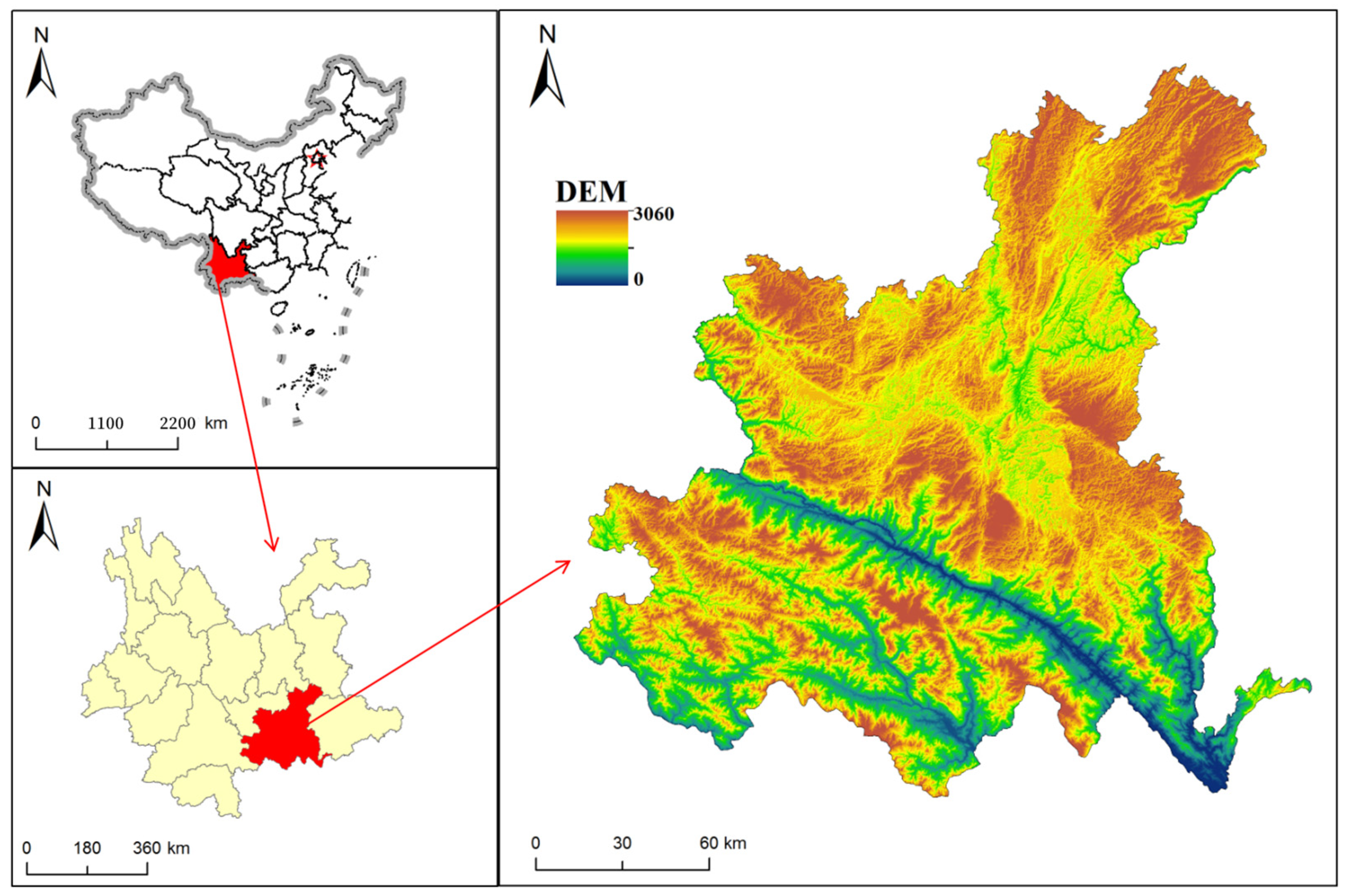
2.1. Study Area

Honghe Autonomous Prefecture is situated in the southern region of Yunnan Province (101°47′–104°16′E, 22°26′–24°45′N), with an area of 32,931 square kilometers. The Honghe River delineates the autonomous prefecture into its northern and southern parts, with mountainous regions constituting 88.5% of the entire expanse. Its climate is a mix of tropical and subtropical monsoons, which result in a non-uniform distribution of rainfall across space and time. The mean annual precipitation stands at 1396.4 mm, with the bulk, 75.9%, occurring between the months of May and October. Forests and cropland are the predominant land use categories, representing 64.40–66.16% and 27.58–30.62% of the total land use, respectively. These are succeeded by grasslands, with building land, water bodies, and unutilized land also figuring into the composition. The distribution of these land use types exhibits a general stability over time. Specifically, forests are predominantly situated in the elevated southern regions, while cropland is concentrated in the central and northern areas. Grasslands are largely found in the central zone, building land is primarily associated with the dam area, water areas are predominantly constituted by lakes and reservoirs, and unutilized land is scattered inconsistently throughout the region (Figure 2).

2.2. Data Sources

The dataset for this research predominantly encompasses land use/cover information, along with meteorological, topographic, soil, vegetation, and socioeconomic data. Detailed information on the data is shown in

Table 1. Overview of the primary data.

Data	Spatial Resolution (m)	Data Source/Processing
Land use/land cover (LULC)	30	Resource and Environmental Science Data Center, Chinese Academy of Sciences (https://www.resdc.cn/, accessed on 1 January 2024)
Digital elevation model (DEM)	30	Geospatial Data Cloud (http://www.gscloud.cn/, accessed on 1 January 2024)
Slope	30	Geospatial Data Cloud (http://www.gscloud.cn/, accessed on 1 January 2024)
Precipitation	30	A Big Earth Data Platform for Three Poles (https://www.geocri.org/data-repositories-tg/big-earth-data-platform-for-three-poles, accessed on 1 January 2024)
Evapotranspiration	1000	A Big Earth Data Platform for Three Poles (https://www.geocri.org/data-repositories-tg/big-earth-data-platform-for-three-poles, accessed on 1 January 2024)
Soil types, soil texture, and organic carbon content	1000	National Tibetan Plateau Science Data Center (https://data.tpdc.ac.cn/, accessed on 1 January 2024)
Normalized difference vegetation index (NDVI)	1000	Resource and Environmental Science Data Center, Chinese Academy of Sciences (https://www.resdc.cn/, accessed on 1 January 2024)
GDP	/	Statistical yearbooks of the counties and districts of Honghe Prefecture
Food yield	/	Statistical yearbooks of the counties and districts of Honghe Prefecture
Population density	/	Statistical yearbooks of the counties and districts of Honghe Prefecture

.

2.3. Assessment of Ecosystem Services

In this study, we systematically identified and categorized ecosystem services based on four key criteria. Initially, we aligned our research with the framework of the Millennium Ecosystem Assessment (MA) to ensure that it encompassed the primary aspects of provisioning, regulating, and supporting services. Subsequently, we carefully selected service types that are crucial to the ecological environment of Yunnan Province, as outlined in the “14th Five-Year Plan for Ecological Environmental Protection in Yunnan Province” released by the Department of Ecology and Environment of Yunnan Province. Thirdly, considering that Honghe Prefecture is a typical karst area, the karst terrain has a series of unique impacts on ecosystem services, especially carbon storage, habitat quality, and soil conservation. Finally, considering the availability and reliability of data, we determined five core services: habitat quality (HQ), carbon storage (CS), soil conservation (SC), water yield (WY), and food production (FP) (

Table 2. Survey of the ecosystem services evaluated in this research.

Category	Ecosystem Service	Abbreviation	Description	Methodology
Supporting service	Habitat quality	HQ	Ecosystems possess the capacity to furnish environments conducive to the sustainability of both individual organisms and their collective populations	InVEST model
Provisioning service	Water yield	WY	The annual yield of water	InVEST model
	Food production	FP	The yield of staple food crops	Measurable proxies
Regulating service	Carbon storage	CS	The quantity of carbon sequestered within terrestrial ecological systems	InVEST model
	Soil conservation	SC	Quantification of soil retention	InVEST model

). These services not only reflect ecological value but are also key indicators for our assessment and protection of the ecological environment. The calculation methods and parameter settings for the values of various ESs were mainly determined according to expert experience, existing research, and the present state of the study area, and the specific methods and steps are detailed in Section S1 [33,34,35,36,37,38,39,40,41].

2.4. Measurement of the Interplay of Trade-Offs and Synergies Between Pairs of ESs

2.4.1. Intercorrelation of ES Groups

The relationships classified as trade-offs and synergies (TOSs) among ESs within the research locale from 2000 to 2020 were ascertained through the application of Spearman’s non-parametric correlation analysis. A synergistic effect is indicated by a positive correlation, while a negative correlation points to a trade-off. The analysis was executed by utilizing the “corrplot” package integrated within the R4.1.2 software environment [42].

2.4.2. Geographically Weighted Regression

To gain a comprehensive grasp of the spatial patterns governing ecosystem services and their TOSs, in this research, the spatial interplay and correlation among trade-offs and synergistic relationships were delineated by employing geographically weighted regression (GWR) [9,43].

2.5. Identification of ES Bundles

The delineation of ES bundles at the grid and township scales was achieved through self-organizing mapping (SOM) and hierarchical bundling (HC). The SOM algorithm functions as an unsupervised neural network for learning processes that bundles multi-dimensional input data and reduces them to a two-dimensional representation while preserving the topological structure of the data. Based on the spatial congruence in the co-occurrence patterns of ESs, these services can be mapped to the neurons closest to them (minimum Euclidean distance), and then HC further divides these secondary bundles into ecosystem service bundles [43]. In using SOM, the ecosystem services of the whole year need to be standardized to ensure the consistency and comparability of ES bundles across various timeframes. The analysis was carried out using the “kohonen” package in R4.1.1 [43].

2.6. Construction of a Comprehensive Ecosystem Service Index

Wang emphasized that considering the trade-offs among the various goals of land administration was deemed essential [7]. The interplay of trade-offs among multiple ESs often reflects the divergent needs and interests among distinct stakeholder groups. Consequently, we implemented an ecosystem service index (ESI) that amalgamates the collective benefits and balances the trade-offs across a spectrum of ESs, thereby providing a holistic representation of their multifaceted values.

The root mean square error (RMSE), a measure derived from the statistical parameters in use, was utilized to quantitatively assess the extent of trade-offs between various ESs. Specifically, the RMSE signifies the variability or tempo of incremental changes occurring unilaterally across different goals, thereby shedding light on the disparities in the rate of ecosystem service alterations moving in a common direction and, thus, broadening the understanding of trade-offs. The specific computational methods are detailed in the referenced literature [5,8].

2.7. Driving Factors and Their Threshold Effects

2.7.1. Natural–Social Factor Selection

ESs represent the interconnected outcomes of natural ecosystems and human society. This study is grounded in preceding research and the procurement of gridded and town-scale data [44,45,46]; we selected nine potential social–ecological factors to evaluate the comparative significance and peripheral effects on five ESs across the research region (

Table 3. Identification of potential socio-ecological factors that impact ESs in Honghe Prefecture.

Type	Group	Driving Factor	Code	Reference
Natural environment	Climate	Aridity index	AI	[47]
		Annual average precipitation	Rain	[48]
	Topography	Slope gradient	Slope	[49]
		Digital elevation model	DEM	[43]
	Vegetation	Normalized difference vegetation index	NDVI	[50]
	Landscape pattern	Landscape disturbance index	LDI	[51]
Socioeconomic system	Social economy	Gross domestic product	GDP	[48]
	Social economy	Population density	POP	[52]
	Land use	Land use	LUI	[53]

). Additionally, we constructed two indices to reflect the relationships of landscape disturbance (LDI) and land use intensity (LUI) with ESs. The calculation formulas and explanations of LDI and LUI are detailed in Section S2.

2.7.2. Relative Importance Assessment

We employed the ArcGIS 10.5 software to compute the average values of putative social and ecological determinants and then implemented a random forest model in the R language’s “Randomforest” to reveal the mechanism driving ESs. The individual socio-ecological factors’ importance regarding ESs is assessed through the percentage rise in the mean squared error of prediction (%IncMSE) [21,54]. The formula for its computation is presented in the following:

$$R{I}_i=in{c}_i/{\displaystyle \sum _{i=1}^{n}in{c}_i}$$

(1)

Here, $R{I}_i$ denotes the significance of the socio-ecological determinant $i$ relative to others; the term $in{c}_i$ is the % IncMSE of factor $i$; n represents the aggregate count of socio-ecological determinants (9 in this study).

2.7.3. Threshold Effect Evaluation

Partial dependence is used to represent the marginal effect of socio-ecological factors on the ESI and to elucidate the nonlinear interconnections between the ESI and natural–social determinants [21]. The formula for its computation is presented in the following:

$$f\left(x_s\right)={\displaystyle \frac{1}{m}}{\displaystyle \sum _{i=1}^{m}f\left(x_s,{x_c}^{\left(i\right)}\right)}$$

(2)

The projected value of an ES is symbolized by $f\left(x_s\right)$; within the socio-ecological framework, $x_s$ represents a factor, while $x_c$ embodies the collection of additional socio-ecological variables used in the random forest model. $x_c$ signifies the volume of data. By averaging across F, the function illustrates the marginal connection between an ES and $x_s$.

3. Results

3.1. Spatial and Temporal Variances in Ecosystem Services

3.1.1. Difference in ESs’ Spatial–Temporal Patterns

The spatial distribution pattern of the five ESs had significant spatial heterogeneity, and it had relative stability in different temporal and spatial scales (Figure 3). Specifically, high values of WY, HQ, CS, and SC were mainly distributed in southern mountainous areas, which were the main distribution areas of woodlands; low values were distributed in the central and northern regions, which were mainly flat basins. The spatial distribution of FP was the opposite of that of the above four ESs. High values of FP were mainly distributed in northern basins, and there was also a spatial concentration of FP in the gentle mountain valleys in southern mountainous areas, which was consistent with the spatial distribution pattern of cultivated land.

The five ESs exhibited pronounced spatial variability yet maintained a degree of consistency across various temporal and spatial dimensions (Figure 3). Notably, the southern mountainous regions, predominantly forested areas, predominantly featured high values for WY, HQ, CS, and SC. Conversely, these values were lower in the central and northern flatlands. In contrast, FP showed an inverse pattern, with high values predominantly in the northern basins and a notable concentration in the southern mountain valleys’ gentle slopes, mirroring the distribution of arable land.

In terms of the time scale, the change rates of the two spatial scales of ESs were similar, but the change trends and speeds of different ESs were different. Overall, in the last 20 years, the total supply of WY, HQ, CS, and SC exhibited a declining trend, whereas FP demonstrated an upward trend. The range of the decline in WY was the highest, followed by that of SC, while HQ and CS showed a slight and continuous decline trend. Specifically, on the grid scale, the supply of WY, HQ, CS, and SC decreased by 61.63%, 37.23%, 2.19%, and 2.15%, respectively, while that of FP increased by 45.58%.

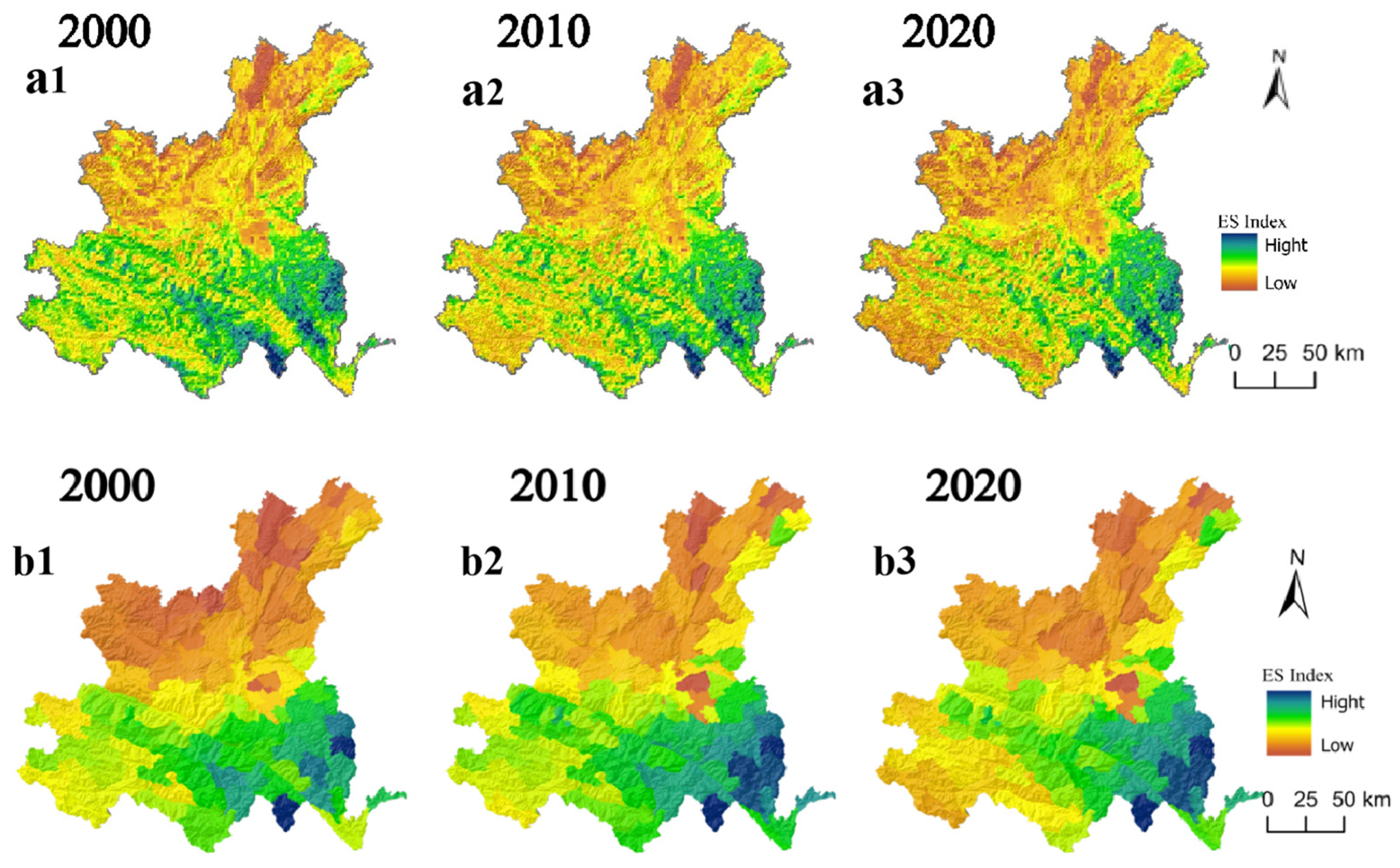
3.1.2. Difference in Spatial–Temporal Patterns of the ESI

At the grid and township scales, the ESI of the study area generally displayed a geographic arrangement characterized as “high in the southern regions and low in the northern areas”. The regions of high-value areas were predominantly located within the mountainous regions to the south. While the areas characterized by lower values were chiefly situated in the northern basins and their surrounding mountains, these regions, despite their lower values, were the main distribution areas for cultivated land and cities (Figure 4).

On the grid scale, the ESI in the southwest exhibited a pronounced decline from 2000 to 2020, indicating that the comprehensive supply capacity of ecosystem services in this region had been degraded. In addition, some areas in the northeast showed an upward trend in the ESI. The spatial distribution pattern of the ESI on the township scale changed over time, and the trend was consistent with that on the grid scale (Figure 4).

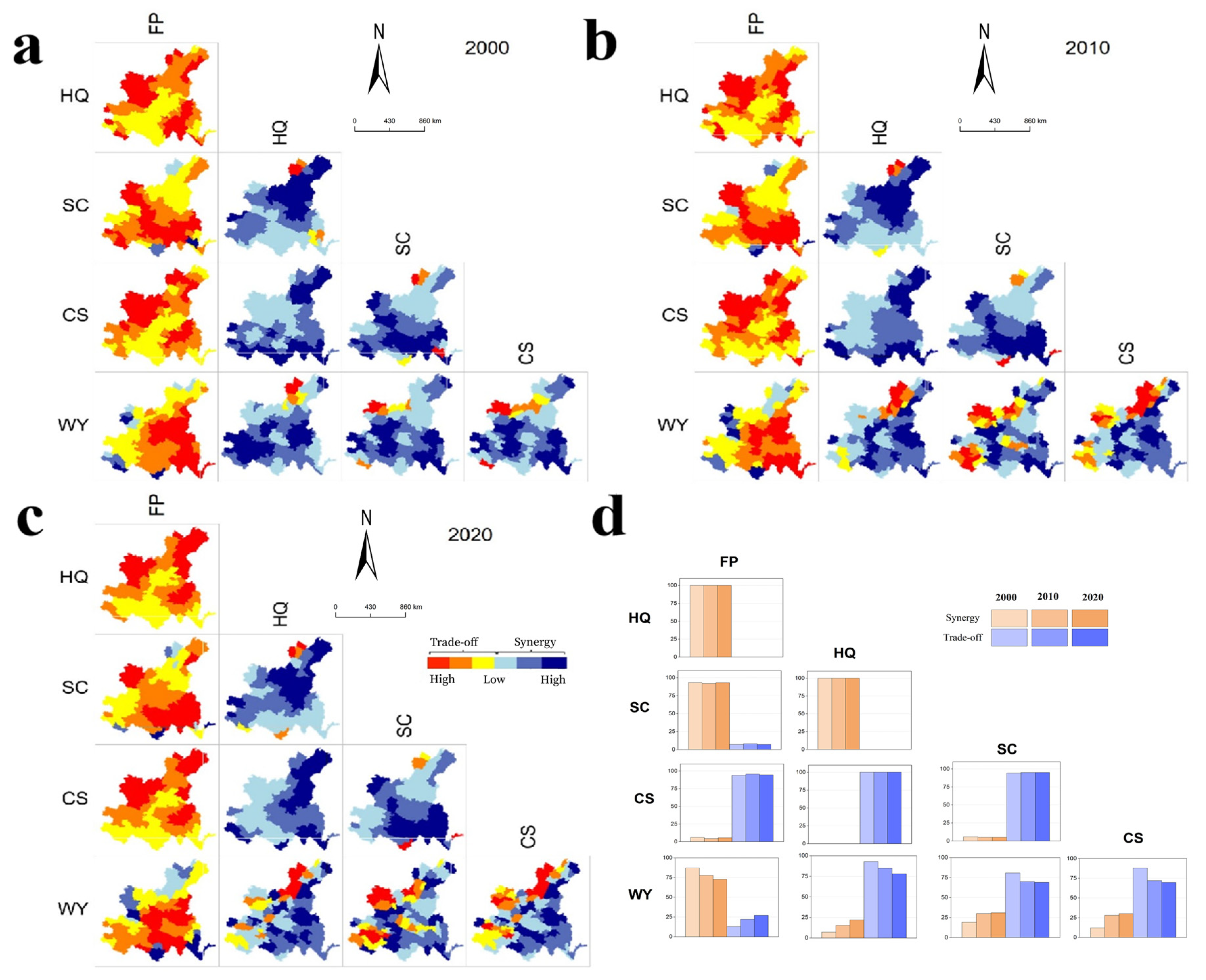
3.2. Differences in Trade-Offs and Synergies of ESs at Different Scales

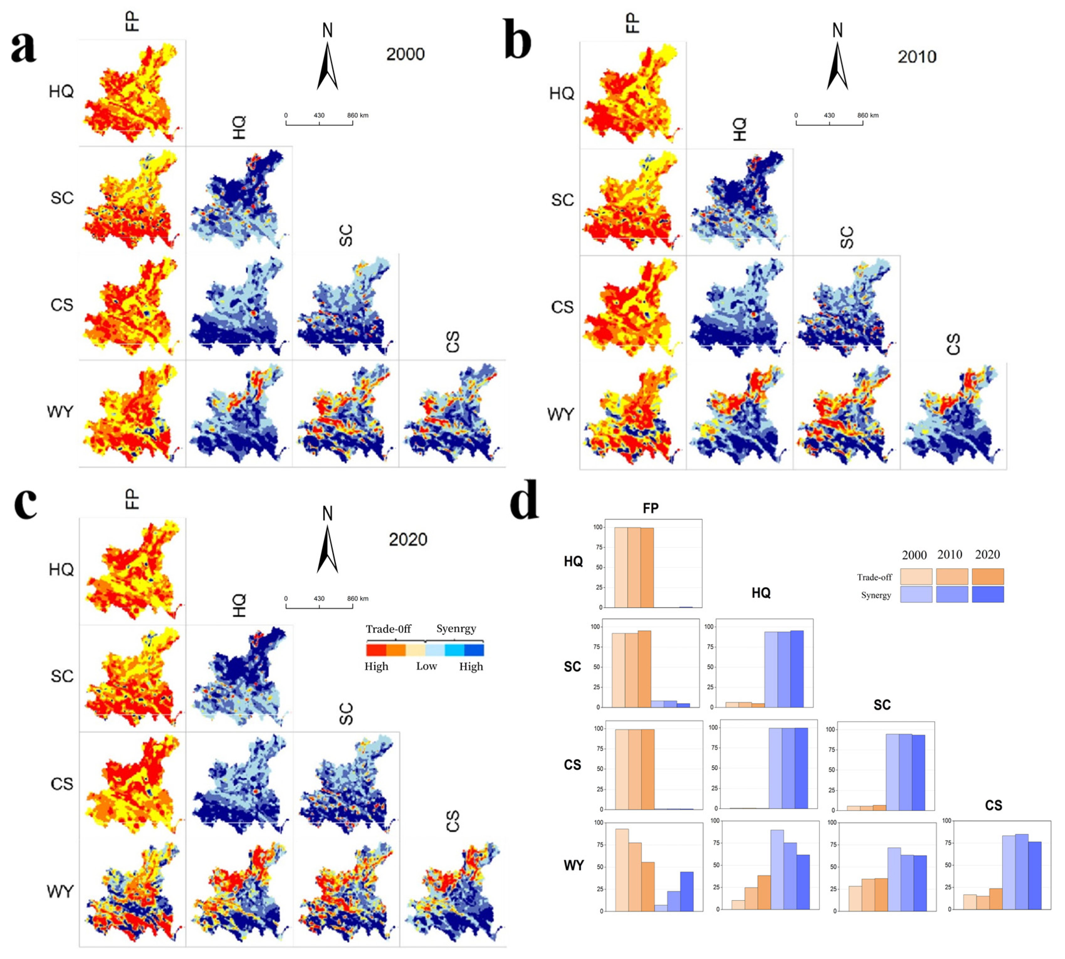
3.2.1. Trade-Offs and Synergies of ES Pairs

Based on the five ES types, we mapped out 30 occurrences of trade-offs and synergies at the grid and township scales, and all of the relationships between ES pairs had statistical significance (p < 0.05) (Figure 5 and Figure 6).

In general, at both the grid and township scales, there were coordination relationships among WY, HQ, CS, and SC, and the ES pairs related to FP all showed trade-off relationships. There were differences in the intensity of trade-offs/coordination among different ES pairs, and the intensity of trade-offs/coordination varied over time. Specifically, HQ and SC, CS, SC, and CS all showed highly coordinated relationships at both scales (ǀrǀ ≥ 0.5), and FP also showed strong trade-off relationships with HQ, SC, and CS (ǀrǀ ≥ 0.5). The correlation coefficients between the grid scale and township scale showed small fluctuations over time.

From a spatial standpoint, the intensity of trade-offs/synergies among ES pairs increased with the scale from the grid scale to the township scale. In terms of the temporal scale, the changes in the intensity of trade-offs/synergies at the two spatial scales remained consistent. The synergy intensity of ES pairs related to WY decreased significantly, while the trade-off effect of ES pairs related to FP could be maintained or even significantly reduced. The correlation indices of other ES pairs increased, but the increase was small. With the change of scale, the intensity changed accordingly, but there was not a directional shift in the trend of trade-offs/synergies.

3.2.2. Spatial and Temporal Characteristics of Trade-Offs and Synergies of ESs

The geographically weighted regression (GWR) examination indicates that the interplay of ESs, characterized by both trade-offs and synergies, displays variability across spatial scales at the grid and township levels (Figure 7 and Figure 8). With an escalation in spatial scale, the subtle distinctions within the trade-offs and synergies of ESs at more detailed scales are diminished, culminating in a distribution that is more consistent across the landscape.

The research indicated that certain combinations of ecosystem services (ESs) exhibited synergistic effects in their spatial interactions, which surpassed the phenomenon of spatial trade-offs. Specifically, the synergistic effects of the ES combinations of SC-HQ, CS-HQ, CS-SC, WY-HQ, WY-SC, and WY-CS were particularly pronounced. The synergies of these areas were mainly concentrated in the southern mountainous region and the northern basin area with its surrounding mountainous areas in the study region. Notably, the strong synergistic areas of SC-HQ were particularly concentrated in the northern part of the study area. On the other hand, the spatial trade-offs of the ES combinations related to FP, such as CS-FP, HQ-FP, SC-FP, and WY-FP, were more prominent, with the proportion of spatial trade-offs exceeding the synergistic effects. The spatial trade-off characteristics of these ES combinations related to FP were mainly reflected in the southern mountainous area, the mountainous area surrounding the northern basin, and the flat valley areas within the region. Further observation revealed that at the township scale, the trade-offs and synergies of ES groups and their spatial distribution patterns were similar to those at the grid scale. ES combinations such as SC-HQ, CS-HQ, CS-SC, WY-HQ, WY-SC, and WY-CS were mainly characterized by synergistic effects, while combinations such as HQ-FP, SC-FP, and CS-FP were primarily characterized by trade-off relationships.

In terms of the temporal trend, there were specific differences in the changes in spatial synergistic/trade-off relationships between ES pairs (Figure 8). From 2000 to 2020, three ES pairs were optimized at the grid scale (increase in the spatial synergy area), and three ES pairs were also optimized at the township scale. At the grid scale, seven pairs of ecosystem services were degraded (increase in the spatial trade-off area), while at the township scale, four pairs of ecosystem services were degraded, and they were all related to WY, including CS-WY, HQ-WY, SC-WY, and WY-FP.

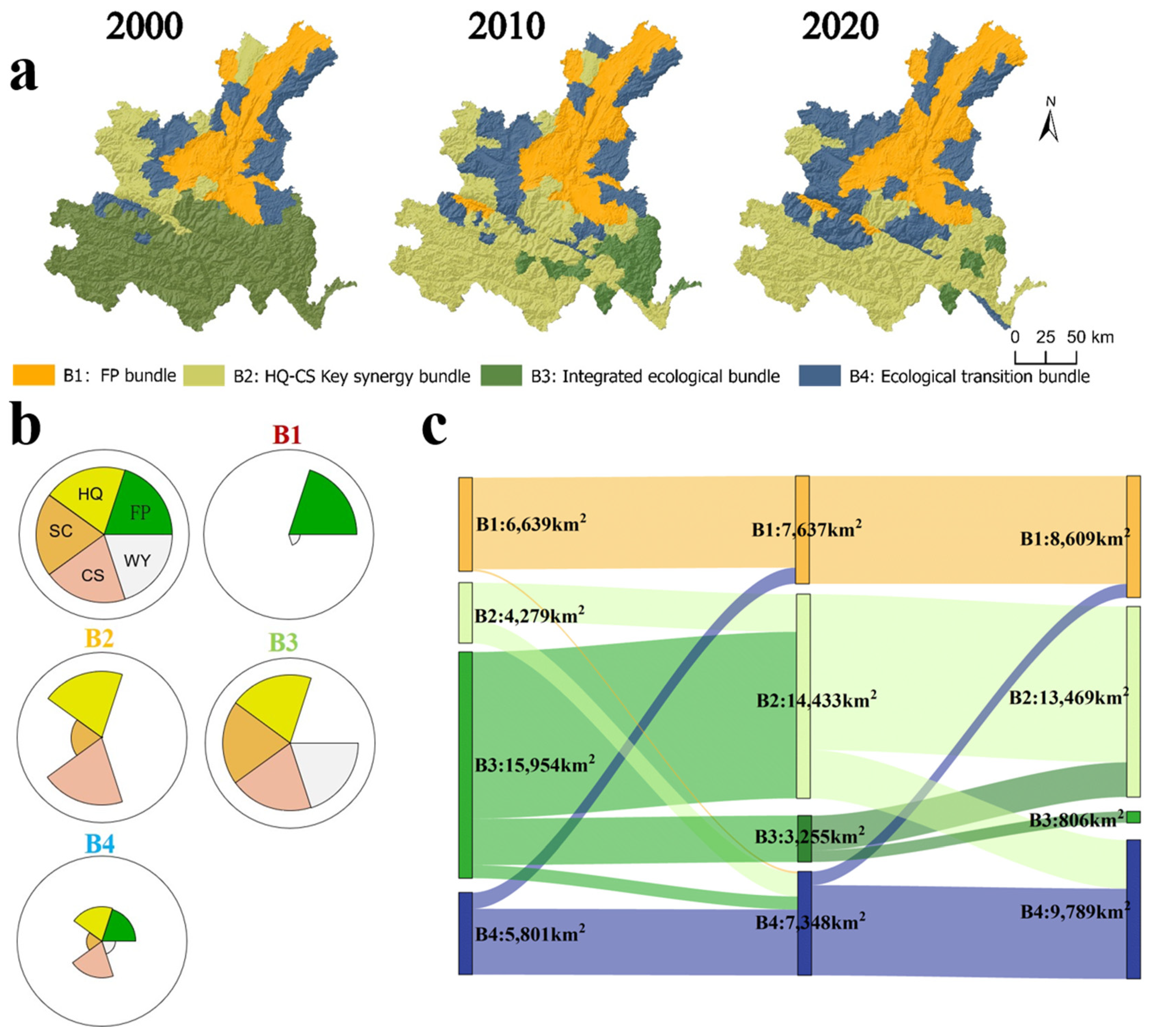
3.3. The Identification of ES Bundles at Different Temporal and Spatial Scales

Four neurons were identified at both the grid scale and township scale in the study area by using SOM. Subsequently, the hierarchical segmentation method was used to further bundle these neurons into four ES bundles (Figure 9 and Figure 10).

At the grid scale, the distinctive features of the four ES bundles can be summarized as follows.

(1)

FP bundle (Bi): This particular bundle was predominantly found in the central and northern sectors of the research locale. The land use type was mainly cropland. It accounted for 16.92%, 19.41%, and 23.14% of the study area in 2000, 2010, and 2020, respectively (Figure 9a,c). This bundle exhibited a spatial collaborative feature of high FP (Figure 9b).

(2)

HQ-CS key synergy bundle (Bii): This bundle predominantly occupied the northwestern and northeastern regions of the study area in 2000, and it was predominantly characterized by forested land, which constituted 15.68% of the total area under investigation. By 2010 and 2020, the distribution of this bundle had shifted predominantly to the northwestern and southwestern parts, representing an increased proportion of the study area at 39.67% and 40.60% (Figure 9a,c). Notably, this bundle demonstrated a spatial synergy with high levels of both HQ and CS (Figure 9b).

(3)

Integrated ecosystem bundle (Biii): This bundle was notably concentrated in the southern mountainous regions of the study area in 2000, accounting for 44.75% of the study area. However, in 2010 and 2020, it was mainly distributed in the southeast, accounting for 11.28% and 5.08% of the study area, respectively (Figure 9a,c). This bundle was characterized by providing multiple ESs, including HQ, SC, CS, and WY (Figure 9b).

(4)

Ecological transition bundle (Biv): In 2000, 2010, and 2020, this bundle was mainly distributed in the transition zone between different bundles, accounting for 22.64%, 29.64%, and 31.19% of the research area, respectively (Figure 9a,c). This bundle showed the characteristics of low ES and frequent changes with other bundles (Figure 9b,c).

At the township scale, the four ES bundles were the same as those at the grid scale, namely, the FP bundle (B1), HQ-CS key synergy bundle (B2), integrated ecological bundle (B3), and ecological transition bundle (B4). The characteristics and spatial distributions of the ES bundles were similar to those at the grid scale, but there were some differences in the spatial distribution and area (Figure 10).

The areas of ecosystem service bundles Bi, Bii, and Biv at the grid scale increased from 2000 to 2010, while the area of Biii decreased. The most significant changes during this period occurred in the transitions of Bii to Biv, Biii to Bii, and Biv to Bi (Figure 9c). In addition, from 2010 to 2020, the areas of Bi, Bii, and Biv expanded, while the area of Biii further shrank. The most significant changes during this period occurred in the transitions of Bii to Biv, Biii to Bii, and Biv to Bi.

The changes in the area of ES bundles at the township scale were basically the same as those at the grid scale. The only difference was that the area of B2 first increased and then decreased. From 2000 to 2020, it accounted for 13.09%, 44.17%, and 41.22% of the study area (Figure 9c).

Through comparison of ES bundles at the grid and township scales, we found that the FP bundle, HQ-CS key synergy bundle, integrated ecological bundle, and ecological transition bundle had similar spatial distribution and area changes at both scales. In particular, from 2000 to 2020, the integrated ecological bundle had largely transformed into the HQ-CS key synergy bundle, which meant that the spatial characteristics of southern mountainous areas in the study area changed from having high-HQ, high-SC, high-CS, and high-WY spatial synergy characteristics to having high-HQ and high-CS spatial synergy characteristics, leading to a decrease in the comprehensive supply capacity of ESs.

The transformation within ES bundles necessitated the development of tailored ES management approaches specifically calibrated to the intended scale of intervention.

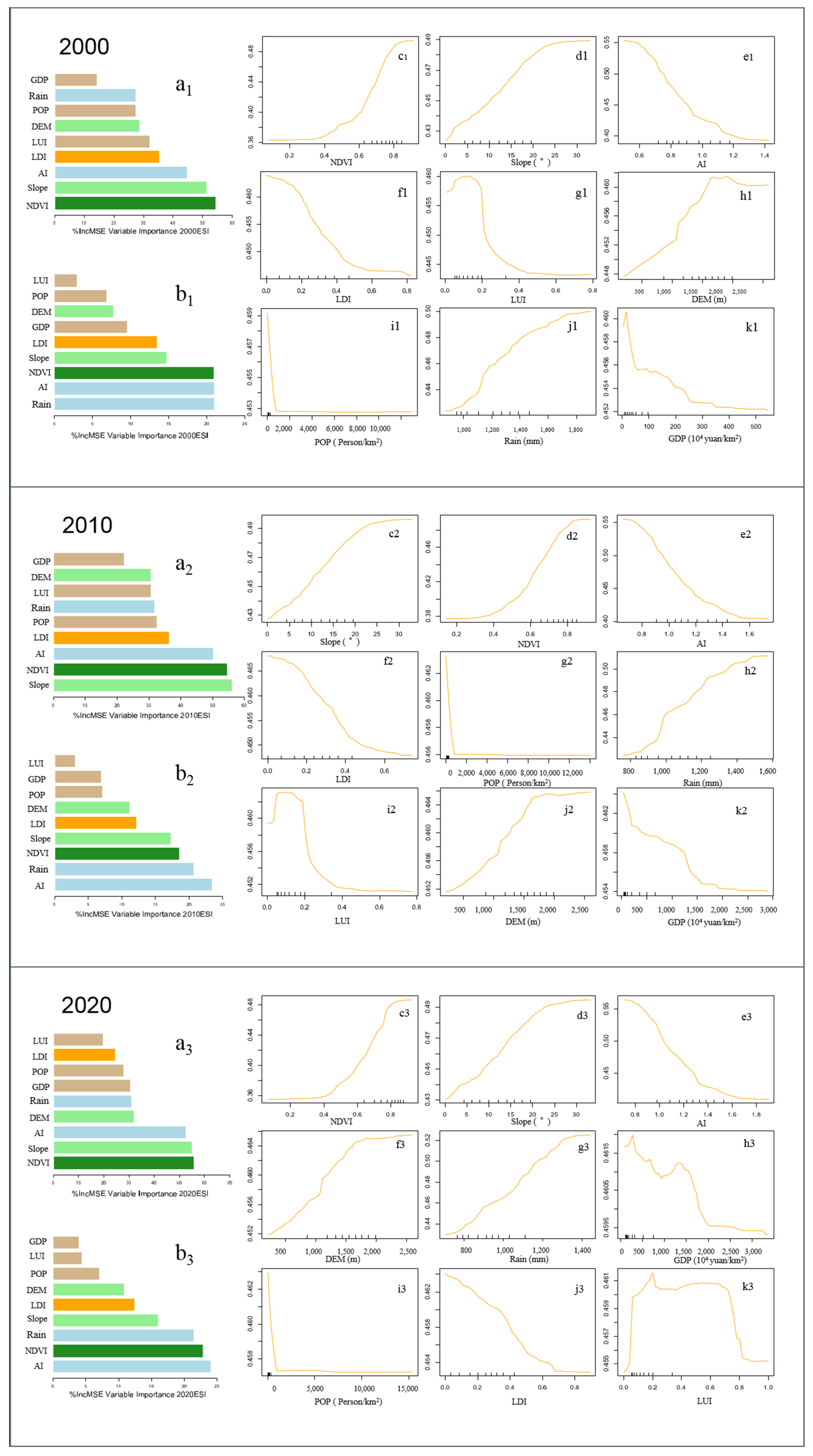
3.4. Threshold Effect of the ESI

At both scales, natural factors were always the most important driving force of the ESI’s spatial heterogeneity. Specifically, on the grid scale, the main driving factors of the ESI’s spatial heterogeneity were vegetation factors (NDVI), terrain factors (Slope), and climate factors (AI), while the differences in the ESI among townships were mainly driven by climate factors (AI, Rain) and vegetation factors (NDVI). This driving difference did not change significantly over time (Figure 11).

In general, natural factors such as the DEM, Slope, NDVI, and Rain played positive driving roles in the spatial differentiation of the ESI, while human activities and AI had negative driving effects on the ESI. However, due to the spatial heterogeneity of natural–social driving factors, the explanatory power of some driving factors on the spatial pattern of the ESI might have shown threshold effects. Specifically, on the grid scale, when the Slope was greater than 20° and the DEM was higher than 1000 m, the response of the ESI to terrain factors became insensitive; the interval of sensitivity of the ESI to the NDVI was 0.6–0.8; when the LDI was greater than 0.6, the response of the ESI to the landscape disturbance index became weak; when the LUI was greater than 0.2, the land use intensity had a negative driving effect on the ESI; the ESI had a higher response sensitivity to POP and GDP. With the increase in POP and GDP, the ESI rapidly decreased and then reached a lower value. With time, the change in the nonlinear relationship between human factors and the ESI became more significant, while the relationship between natural factors and the ESI was relatively stable. The grid scale and township scale showed similar nonlinear relationships, but there were differences in their thresholds (Figure 11 and Section S3).

4. Discussion

4.1. Spatial–Temporal Patterns of ES Supply and Their Interactions

We characterized the relationships among ESs as either synergistic or indicative of trade-offs, which are integral to the concept of ES bundles. Grasping the intricate interplay among these ESs is essential for the prudent management of ESs [9]. The geographic congruence of diverse ES forms results in the creation of distinct ES bundles, which are essential for the effective joint stewardship of various ecological services [11,12,55]. ESs have spatial heterogeneity, which is typically associated with the varied spatial distribution of natural–social factors.

In terms of spatial distribution, HQ, WY, CS, SC, FP, and ESI exhibited comparable spatial arrangement patterns. Regions with elevated ES supply were predominantly located in areas characterized by mountains and hills. The regions in question, characterized by their extensive and unbroken natural and semi-natural forest landscapes, serve as vital carbon sinks and provide complete habitats [56,57]. Their high altitudes and complex topography facilitate the uplift of moist air currents, resulting in generous rainfall [58]. The elevation also contributes to reduced rates of evapotranspiration, which, in turn, enhances the water retention capacity of these areas. Consequently, these topographical and climatic attributes are instrumental in the regions’ notable capacity for water supply and conservation. Moreover, the challenging mountainous terrain deters the concentration of dense populations and intensive economic activities, thereby preserving a stable ecological state. This state is marked by high habitat quality and robust vegetation cover, which are essential for the efficient co-management of multiple ecosystem services. The preservation of these natural conditions is crucial for sustaining the ecological integrity and the delivery of services that these regions provide [56,57,58,59]. Therefore, the synergy mainly occurred among HQ, WY, CS, and SC, further making the ES bundles present in the form of the HQ-CS key synergy bundle and integrated ecological bundle, with strong supply capacity at the grid and township scales. This concordance in synergies among ESs aligns with the findings of prior scholarly work [9,60,61,62].

Conversely, the northern region’s plains exhibit lower elevations, level landscapes, and a pervasive and concentrated arrangement of arable land, urban centers, and rural settlements. It is also the main grain supply area and population distribution area in the Red River region. This area shows a spatial pattern of high FP supply and low supply of other ESs. In this area, FP and other ESs are generally characterized by trade-offs, which are intricately associated with the dynamics of land use conflicts, particularly highlighting the contentious issue between areas designated for agriculture and those maintained as forests [63,64]. Land use conflicts underscore the incompatibility of allocating a single parcel of land for exclusive use by one ecosystem over another [64]. Farmland often has a high capacity for food production, but it has poor abilities for support and regulation, making it the opposite of forests [65]. Within the scope of that research, the scarcity of pristine or semi-pristine habitats coupled with the escalating intensity of anthropogenic actions resulted in a trade-off between FP and other ESs in the specified area. The inclination towards FP is intimately connected to the immediate human demand for an escalation in the food production sector during rapid urbanization processes [64]. In previous studies on functional zones of ESs, that area was defined as a separate FP bundle, highlighting the necessity of evaluating the balance between FP and the various components of ESs [63,66]. Consequently, upcoming conservation measures should tackle the trade-offs between FP and other ESs in order to alleviate the decline of natural habitats due to the progression of intensive farming, thus averting the adverse enduring consequences for sustainability and the welfare of human societies [62,67].

Furthermore, our research also explored the temporal changes in the interactions among ESs. We found that on both the grid scale and the township scale, the synergy of ES pairs related to WY (WY-HQ, WY-SC, WY-CS) decreased, and at the same time, the spatial synergy of these ES pairs decreased, leading to a wider spatial trade-off. The weaker synergy of WY-related ES pairs might have been associated with the variability in climatic elements, including precipitation [66]. The significant unpredictability in rainfall amounts has led to variability in the water provision for these two hydrological ESs, which further weakened the synergy of WY-related ESs. The fluctuations in precipitation and the unpredictability of WY have escalated the uncertainty regarding water security within the research locale [65]. At the same time, while the supply of FP increased year by year, the trade-off effect of the FP-related ES pairs (FP-HQ, FP-CS, FP-WY) could maintain stability or even significantly decrease. The spatial trade-off effect of these ES pairs was reduced, making the spatial synergy expand. The decrease in the trade-off between FP and HQ, CS, and WY might have been related to changes in the supply and demand of FP [68,69]. With the advancement of agricultural technology and the adjustment of agricultural structure, the supply efficiency of FP was improved, and the demand elasticity of FP was decreased, resulting in weaker competition between FP and HQ, CS, and WY. These findings underscore the significance of ES pairs that exhibit diminished synergistic/trade-off effects in the realm of ES management, which are effects that can often be obscured within the scope of individual studies [64,69]. Therefore, it is crucial to conduct a time-based analysis to identify pairs of ESs that exhibit diminished synergistic impacts and to give precedence to their recognition in an ecosystem service management plan.

4.2. The Threshold Effect of the ESI’s “Natural–Social” Driving Factors

Thresholds are delineated as pivotal junctures of adaptation within the nexus of ecosystem conditions and their propelling elements at which minor alterations in determinant factors can provoke substantial variations in the ecosystem’s status and its ability to furnish ESs [20,70]. Therefore, it is necessary to analyze the driving factors of the spatial differentiation of ESs and establish their status as a priority area within the realm of ES management [21,22].

In this study, we explored whether there was a threshold effect of the driving factors of the spatial differentiation of the ESI and its significance for ecological management. Specifically, topographic factors (DEM, Slope) and vegetation factors (NDVI) play a positive role in the spatial differentiation of the ESI. As population and economic activities tend to gather in low-altitude and gentle areas, human disturbance is small and vegetation coverage is high in high-altitude and steep areas. The ecosystem has high water conservation, soil conservation, and other service functions, so the value of the ESI is higher [56,71]. However, this kind of relationship is not linear. When the altitude and slope exceed certain values, the growth conditions of the ecosystem become poor, the coverage and diversity of vegetation decrease, and the stability and resistance of the ecosystem to interference decrease [21,72]. Therefore, the ESI value no longer increases with the increase in altitude and slope, but it tends to be stable at a higher level [73]. Honghe is a typical karst region in southwest China, where the terrain’s spatial differences are relatively large, and the ESI’s response to the terrain is sensitive. Therefore, in mountainous areas with large terrain fluctuations, we should strengthen ecological protection and restoration and maintain the high service function of the ecosystem while avoiding over-exploitation and utilization and preventing the degradation and collapse of the ecosystem [71,74].

The landscape disturbance index (LDI) reflects the damage degree of human activities on the ecosystem. High landscape disturbance will lead to the degradation and loss of the function of an ecosystem, thus reducing the value of the ESI. When the landscape disturbance index exceeds a certain value, the ecosystem has reached a lower equilibrium state, and it is difficult to further decline [22,73,75,76]. Therefore, the ESI does not decrease with the increase in the landscape disturbance index, but it tends to be stable or to slightly rebound. The intensity of land use (LUI) follows a similar pattern to that of LUI, but in the lower range of LUI, land development and utilization can actually bring positive ecological benefits [73,77]. For instance, well-managed agricultural practices can enhance biodiversity, which, in turn, can lead to an improvement in the ecosystem service index (ESI). Moreover, moderate levels of land use can contribute to better soil quality, further enhancing the ESI [78]. Therefore, in regions with high human activity intensity, it is imperative to formulate land development plans that are scientifically grounded and sustainable. These plans should prioritize the limitation of urban and agricultural expansion into areas designated as ecological land, thereby preserving critical habitats and ecosystem functions. Reducing landscape disturbance and destruction is essential, as it helps to maintain the structural and functional integrity of ecosystems [77]. These results highlight the threshold effect of natural–social factors on ES management, which is easily concealed in linear correlation analysis.

4.3. The Spatial Scale Effect of ES Interactions

ES management requires a comprehension of the complex interplay of ecological interactions and the integration of scaling effects within these ES interactions [3,4]. We constructed scales for ES assessment at the township and grid scales to facilitate ES management at different spatial scales. In addition, we concentrated our research on four dimensions of the spatial scale’s impact on ecosystem services, namely, how the scale influences (1) the spatial patterns of ESs, (2) the trade-offs/synergies of ESs, (3) the ES bundles, and (4) the driving factors of ESs. The spatial patterns of ESs are relatively stable at different scales, which aligns with the conclusions drawn from additional scholarly investigations [23,24,27,79]. However, the scale of ESs had a significant impact on trade-offs/synergies. Firstly, we found that at the township scale, the absolute values of the correlation coefficients are always greater than those for the same ES pairs at the grid scale. This result is supported by Xia and Yuan [43], who demonstrated that synergies increase with increasing scale. Secondly, the change in scale did not alter the trade-offs/synergies of ES pairs. Results from other studies similarly indicated that the relationships between ESs are robust at different scales [9,14,18]. Thirdly, the strength of trade-offs/synergies of ES pairs was similar at different scales [15,43]; for example, CS-HQ demonstrates the strongest synergistic effects across both scales, whereas FP-HQ exhibits the strongest trade-offs at both scales. Fourthly, trade-offs/synergies of ES pairs may not spatially match at different scales. The variations and intensities of relationships at different scales demonstrated the complexity of trade-offs/synergies of ESs at different scales [9]. With alterations in temporal or spatial scales, the predictability of trade-offs diminishes, complicating their management. The scale-related impacts on ecosystem service (ES) interactions are unique to the context and are markedly shaped by the regional biophysical and socioeconomic milieu [43]. Accordingly, ES-focused studies across various geographic locales should correlate scale effects with their respective geographic contexts to furnish insights for ecosystem management that transcends scales and promotes sustainable spatial planning.

Our results revealed the temporal and scale variations of ES bundles and their natural–social drivers. Raudsepp-Hearne and Peterson [27] also illustrated the resilience of ES bundles at finer scales but observed variations at broader scales. Furthermore, our findings revealed disparities in the principal determinants of ESs across various scales, suggesting that socio-ecological factors that are pivotal at one scale could diminish in significance or become inconsequential at another [4,80]. Service-providing units refer to the fundamental physical units capable of generating specific ESs, and the spatial patterns of natural–social factors within different service-providing units vary with changing scales [24,81]. With the expansion of the spatial scale, certain categories of service-providing entities may consolidate, creating alternative types of entities with distinct attributes of natural–social factors and diverse abilities to furnish ESs. Therefore, changes in the spatial scale can alter the associations and strengths between ESs and natural–social drivers [43,81]. These differences can easily be masked in single-scale studies. Hence, this necessitates the development of tailored sustainable management strategies for ESs that are adapted to distinct scales.

4.4. Multi-Scale Management of Regional ESs Based on the Perspective of “Supply–Interaction–Drive–Threshold”

The patterns, interactions, and drivers of ESs exhibit spatial variability, implying that governance choices for ESs at one spatial scale may not be suitable for other scales [4,23]. This complexity of spatial management is reflected in the differences in ESs’ relationships across different spatial scales in Honghe Prefecture. Therefore, understanding the supply, interactions, and thresholds of ESs in relation to natural–social drivers requires a multi-scale perspective, which is essential for conducting multi-level regional ecological management [23,27,79]. Based on this concept, we developed a regional ES management framework that adopted a multi-scale “supply–interaction–driver–threshold” perspective. This framework provided a more comprehensive view of regional ES management.

The overall distribution of the ESI in the study area shows a spatial pattern where the southern mountainous regions exhibit significantly higher values than the northern basin and hilly areas. Over a period of 20 years, the comprehensive supply capacity of ESs in the southwestern mountainous regions significantly decreased, with this degradation also being reflected in the widespread transition from the integrated ecological bundle to the HQ-CS key synergy bundle. Therefore, we recommend delineating ecological spatial management boundaries based on ES bundles and implementing specific ecological protection policies targeting the integrated ecological bundle and the HQ-CS key synergy bundle in the southern mountainous regions to reverse this degradation trend. Specifically, (1) for the already degraded former “integrated ecological bundle” areas, we should implement ES restoration policies targeting SC and WY. For example, at both scales, topographic factors and meteorological factors consistently serve as the primary drivers of SC (Section S3), so measures such as restricting slope development, implementing the conversion of land into forests, and constructing drainage systems should be taken to reduce soil erosion. At the grid scale, it is necessary to limit the impact of human activities on WY. This can be achieved by restricting urban and agricultural encroachment on ecological land, as well as reducing landscape disturbance and destruction to restore the integrity and stability of the ecosystem. At the township scale, ecological governance should fully consider the influence of climate factors and develop ecological governance strategies that are adapted to local climatic conditions. For example, improving irrigation facilities to enhance water resource utilization efficiency or planting plant species that are adapted to local rainfall conditions can improve the adaptive capacity of the ecosystem. (2) For the existing “integrated ecological bundle” areas, which have the strongest comprehensive ES supply capacity, measures should be taken to further restrict human disturbances to prevent degradation. Ecological conservation areas can be designated to maintain their stable state.

The northern region is the most populated and economically concentrated area, and it is the main distribution area of the ecological transition bundle and the FP bundle. ES trade-offs also primarily occur in the northern region, where the comprehensive supply capacity of the ESI is lower, and human activities are the main driving factors for FP (Section S3). Considering the local economic and social development needs, an ecological policy focused on improvement should be implemented in this area. Specifically, we suggest updating the ecological agricultural production mode to improve the supply capacity of FP while mitigating the trade-off effects with other ESs. Increasing vegetation coverage on the basis of preserving the bottom line of basic farmland can enhance the supply of regulating services and supporting services. Adjusting the land use structure can reduce the pressure of land development and landscape disturbance on the supply of other ESs.

4.5. Limitations and Prospects of Research

This research furnishes analytical insights and a conceptual foundation for the management of ESs from multiple perspectives, but it also has some limitations. Firstly, when calculating the five ecosystem services, the commonly used models and formulas are adopted, and there is a lack of measured data for verification. In addition, owing to the clarity and fidelity of remote sensing images, discrepancies may arise. Secondly, when characterizing the trade-off/synergistic relationships and intensities between services, Spearman’s non-parametric correlation analysis focuses on the evaluation of trade-off relationships between paired ecosystem services, and there are differences in the interpretation of results compared with other analysis methods. In subsequent studies, various analysis methods should be adopted and compared, such as the root mean square deviation method and relative change method. Finally, this study makes a significant original contribution to the field of ecosystem service management, especially in the specific geographical context of the karst terrain region of Honghe Prefecture in Yunnan. This study adopts a multi-dimensional “supply–interaction–driver–threshold” perspective to construct an integrated cognitive framework, which has not been fully explored in previous studies. This framework not only deepens the understanding of the complex interactions of ecosystem services and their nonlinear relationships with natural–social factors but also provides a more comprehensive theoretical support and original contribution to regional ecosystem service management.

5. Conclusions

This study used the karst region of Yunnan’s Honghe Prefecture as a case study to conduct an in-depth analysis of the spatiotemporal heterogeneity, interactions, and driving factors of ESs, along with their threshold effects. The results indicated significant spatial variations in ecosystem services, with an enhancement in the FP capacity and a decline in WY. Synergies were primarily observed among habitat quality, carbon storage, and soil retention, while trade-offs existed between FP and other services. Changes in the ES bundles in the southern mountainous areas underscored the importance of the spatial scale in management. By constructing an ESI, it was discovered that human activities and climate aridity were the main factors impacting it, and a threshold effect was revealed, suggesting that ecosystem service responses might undergo nonlinear changes under specific conditions. Based on the study’s findings, it was proposed that ecological protection policies should be implemented in the southern mountainous areas to reverse the trend of degradation; northern areas should update their ecological agriculture models to balance food production with other services. This study highlighted the importance of spatiotemporal scales and threshold effects in the management of ecosystem services, offering a basis for the development of scientific management strategies.

References

1. Abernethy, V.D. Nature’s Services: Societal Dependence on Natural Ecosystems. Popul. Environ. 1999, 20, 277–278. [Google Scholar] [CrossRef]
2. Bennett, E.M.; Peterson, G.D.; Gordon, L.J. Understanding Relationships among Multiple Ecosystem Services. Ecol. Lett. 2009, 12, 1394–1404. [Google Scholar] [CrossRef]
3. Zhang, Z.; Liu, Y.; Wang, Y.; Liu, Y.; Zhang, Y.; Zhang, Y. What Factors Affect the Synergy and Tradeoff between Ecosystem Services, and How, from a Geospatial Perspective? J. Clean. Prod. 2020, 257, 120454. [Google Scholar] [CrossRef]
4. Shen, J.; Li, S.; Liu, L.; Liang, Z.; Wang, Y.; Wang, H.; Wu, S. Uncovering the Relationships between Ecosystem Services and Social-Ecological Drivers at Different Spatial Scales in the Beijing-Tianjin-Hebei Region. J. Clean. Prod. 2021, 290, 125193. [Google Scholar] [CrossRef]
5. Wang, C.; Tang, C.; Fu, B.; Lü, Y.; Xiao, S.; Zhang, J. Determining Critical Thresholds of Ecological Restoration Based on Ecosystem Service Index: A Case Study in the Pingjiang Catchment in Southern China. J. Environ. Manag. 2022, 303, 114220. [Google Scholar] [CrossRef] [PubMed]
6. Liu, L.; Zhang, H.; Gao, Y.; Zhu, W.; Liu, X.; Xu, Q. Hotspot Identification and Interaction Analyses of the Provisioning of Multiple Ecosystem Services: Case Study of Shaanxi Province, China. Ecol. Indic. 2019, 107, 105566. [Google Scholar] [CrossRef]
7. Wu, L.; Fan, F. Assessment of Ecosystem Services in New Perspective: A Comprehensive Ecosystem Service Index (CESI) as a Proxy to Integrate Multiple Ecosystem Services. Ecol. Indic. 2022, 138, 108800. [Google Scholar] [CrossRef]
8. Zhu, Q.; Cai, Y. Integrating Ecological Risk, Ecosystem Health, and Ecosystem Services for Assessing Regional Ecological Security and Its Driving Factors: Insights from a Large River Basin in China. Ecol. Indic. 2023, 155, 110954. [Google Scholar] [CrossRef]
9. Liu, Q.; Qiao, J.; Li, M.; Huang, M. Spatiotemporal Heterogeneity of Ecosystem Service Interactions and Their Drivers at Different Spatial Scales in the Yellow River Basin. Sci. Total Environ. 2024, 908, 168486. [Google Scholar] [CrossRef] [PubMed]
10. Meacham, M.; Norstrom, A.; Peterson, G.D.; Andersson, E.; Bennett, E.M.; Biggs, R.; Crouzat, E.; Cord, A.F.; Enfors, E.; Felipe-Lucia, M.R.; et al. Advancing Research on Ecosystem Service Bundles for Comparative Assessments and Synthesis. Ecosyst. People 2022, 18, 99–111. [Google Scholar] [CrossRef]
11. Raudsepp-Hearne, C.; Peterson, G.D.; Bennett, E.M. Ecosystem Service Bundles for Analyzing Tradeoffs in Diverse Landscapes. Proc. Natl. Acad. Sci. USA 2010, 107, 5242–5247. [Google Scholar] [CrossRef] [PubMed]
12. Harris, L.R.; Defeo, O. Sandy Shore Ecosystem Services, Ecological Infrastructure, and Bundles: New Insights and Perspectives. Ecosyst. Serv. 2022, 57, 101477. [Google Scholar] [CrossRef]
13. Feng, Q.; Zhao, W.; Hu, X.; Liu, Y.; Daryanto, S.; Cherubini, F. Trading-off Ecosystem Services for Better Ecological Restoration: A Case Study in the Loess Plateau of China. J. Clean. Prod. 2020, 257, 120469. [Google Scholar] [CrossRef]
14. Qin, K.; Li, J.; Yang, X. Trade-Off and Synergy among Ecosystem Services in the Guanzhong-Tianshui Economic Region of China. Int. J. Environ. Res. Public Health 2015, 12, 14094–14113. [Google Scholar] [CrossRef]
15. Stosch, K.C.; Quilliam, R.S.; Bunnefeld, N.; Oliver, D.M. Quantifying Stakeholder Understanding of an Ecosystem Service Trade-Off. Sci. Total Environ. 2019, 651, 2524–2534. [Google Scholar] [CrossRef] [PubMed]
16. Kong, L.; Zheng, H.; Xiao, Y.; Ouyang, Z.; Li, C.; Zhang, J.; Huang, B. Mapping Ecosystem Service Bundles to Detect Distinct Types of Multifunctionality within the Diverse Landscape of the Yangtze River Basin, China. Sustainability 2018, 10, 857. [Google Scholar] [CrossRef]
17. Cai, W. Identifying Ecosystem Services Bundles for Ecosystem Services Trade-Off/Synergy Governance in an Urbanizing Region. Land 2022, 11, 1593. [Google Scholar] [CrossRef]
18. Cheng, X.; Xu, Z.; Yu, S.; Peng, J. A Wavelet Coherence Approach to Detecting Ecosystem Services Trade-off Response to Land Use Change. J. Environ. Manag. 2022, 316, 115160. [Google Scholar] [CrossRef]
19. Peng, J.; Tian, L.; Liu, Y.; Zhao, M.; Hu, Y.; Wu, J. Ecosystem Services Response to Urbanization in Metropolitan Areas: Thresholds Identification. Sci. Total Environ. 2017, 607, 706–714. [Google Scholar] [CrossRef] [PubMed]
20. Ma, S.; Wang, L.-J.; Jiang, J.; Chu, L.; Zhang, J.-C. Threshold Effect of Ecosystem Services in Response to Climate Change and Vegetation Coverage Change in the Qinghai-Tibet Plateau Ecological Shelter. J. Clean. Prod. 2021, 318, 128592. [Google Scholar] [CrossRef]
21. Wu, J.; Guo, X.; Zhu, Q.; Guo, J.; Han, Y.; Zhong, L.; Liu, S. Threshold Effects and Supply-Demand Ratios Should Be Considered in the Mechanisms Driving Ecosystem Services. Ecol. Indic. 2022, 142, 109281. [Google Scholar] [CrossRef]
22. Ran, Z.; Gao, S.; Zhang, B.; Guo, C.; Ouyang, X.; Gao, J. Non-Linear Effects of Multi-Dimensional Urbanization on Ecosystem Services in Mega-Urban Agglomerations and Its Threshold Identification. Ecol. Indic. 2023, 154, 110846. [Google Scholar] [CrossRef]
23. Cord, A.F.; Bartkowski, B.; Beckmann, M.; Dittrich, A.; Hermans-Neumann, K.; Kaim, A.; Lienhoop, N.; Locher-Krause, K.; Priess, J.; Schroeter-Schlaack, C.; et al. Towards Systematic Analyses of Ecosystem Service Trade-Offs and Synergies: Main Concepts, Methods and the Road Ahead. Ecosyst. Serv. 2017, 28, 264–272. [Google Scholar] [CrossRef]
24. Zheng, D.; Wang, Y.; Hao, S.; Xu, W.; Lv, L.; Yu, S. Spatial -Temporal Variation and Tradeoffs/Synergies Analysis on Multiple Ecosystem Services: A Case Study in the Three -River Headwaters Region of China. Ecol. Indic. 2020, 116, 106494. [Google Scholar] [CrossRef]
25. Lautenbach, S.; Kugel, C.; Lausch, A.; Seppelt, R. Analysis of Historic Changes in Regional Ecosystem Service Provisioning Using Land Use Data. Ecol. Indic. 2011, 11, 676–687. [Google Scholar] [CrossRef]
26. Deng, X.; Li, Z.; Gibson, J. A Review on Trade-off Analysis of Ecosystem Services for Sustainable Land-Use Management. J. Geogr. Sci. 2016, 26, 953–968. [Google Scholar] [CrossRef]
27. Raudsepp-Hearne, C.; Peterson, G.D. Scale and Ecosystem Services: How Do Observation, Management, and Analysis Shift with Scale-Lessons from Quebec. Ecol. Soc. 2016, 21, 16. [Google Scholar] [CrossRef]
28. Li, M.; Zheng, P.; Pan, W. Spatial-Temporal Variation and Tradeoffs/Synergies Analysis on Multiple Ecosystem Services: A Case Study in Fujian. Sustainability 2022, 14, 3086. [Google Scholar] [CrossRef]
29. Liao, C.; Yue, Y.; Wang, K.; Fensholt, R.; Tong, X.; Brandt, M. Ecological Restoration Enhances Ecosystem Health in the Karst Regions of Southwest China. Ecol. Indic. 2018, 90, 416–425. [Google Scholar] [CrossRef]
30. Tong, X.; Wang, K.; Yue, Y.; Brandt, M.; Liu, B.; Zhang, C.; Liao, C.; Fensholt, R. Quantifying the Effectiveness of Ecological Restoration Projects on Long-Term Vegetation Dynamics in the Karst Regions of Southwest China. Int. J. Appl. Earth Obs. Geoinf. 2017, 54, 105–113. [Google Scholar] [CrossRef]
31. Peng, J.; Yang, Y.; Liu, Y.; Hu, Y.; Du, Y.; Meersmans, J.; Qiu, S. Linking Ecosystem Services and Circuit Theory to Identify Ecological Security Patterns. Sci. Total Environ. 2018, 644, 781–790. [Google Scholar] [CrossRef] [PubMed]
32. Zhang, W.; Yu, Y.; Wu, X.; Pereira, P.; Borja, M.E.L. Integrating Preferences and Social Values for Ecosystem Services in Local Ecological Management: A Framework Applied in Xiaojiang Basin Yunnan Province, China. Land Use Pol. 2020, 91, 104339. [Google Scholar] [CrossRef]
33. Sun, X.; Lu, Z.; Li, F.; Crittenden, J.C. Analyzing Spatio-Temporal Changes and Trade-Offs to Support the Supply of Multiple Ecosystem Services in Beijing, China. Ecol. Indic. 2018, 94, 117–129. [Google Scholar] [CrossRef]
34. Pan, H.; Du, Z.; Wu, Z.; Zhang, H.; Ma, K. Assessing the Coupling Coordination Dynamics between Land Use Intensity and Ecosystem Services in Shanxi’s Coalfields, China. Ecol. Indic. 2024, 158, 111321. [Google Scholar] [CrossRef]
35. Zhang, S.; Xiong, K.; Qin, Y.; Min, X.; Xiao, J. Evolution and Determinants of Ecosystem Services: Insights from South China Karst. Ecol. Indic. 2021, 133, 108437. [Google Scholar] [CrossRef]
36. Shen, J.; Li, S.; Liang, Z.; Liu, L.; Li, D.; Wu, S. Exploring the Heterogeneity and Nonlinearity of Trade-Offs and Synergies among Ecosystem Services Bundles in the Beijing-Tianjin-Hebei Urban Agglomeration. Ecosyst. Serv. 2020, 43, 101103. [Google Scholar] [CrossRef]
37. Kuriqi, A.; Pinheiro, A.N.; Sordo-Ward, A.; Garrote, L. Influence of Hydrologically Based Environmental Flow Methods on Flow Alteration and Energy Production in a Run-of-River Hydropower Plant. J. Clean. Prod. 2019, 232, 1028–1042. [Google Scholar] [CrossRef]
38. Liu, M.; Xiong, Y.; Zhang, A. Multi-Scale Telecoupling Effects of Land Use Change on Ecosystem Services in Urban Agglomerations–A Case Study in the Middle Reaches of Yangtze River Urban Agglomerations. J. Clean. Prod. 2023, 415, 137878. [Google Scholar] [CrossRef]
39. Zhang, B.; Zheng, L.; Wang, Y.; Li, N.; Li, J.; Yang, H.; Bi, Y. Multiscale Ecosystem Service Synergies/Trade-Offs and Their Driving Mechanisms in the Han River Basin, China: Implications for Watershed Management. Environ. Sci. Pollut. Res. 2023, 30, 43440–43454. [Google Scholar] [CrossRef]
40. Gao, Z.-Q.; Tao, F.; Wang, Y.-H.; Zhou, T. Potential Ecological Risk Assessment of Land Use Structure Based on MCCA Model: A Case Study in Yangtze River Delta Region, China. Ecol. Indic. 2023, 155, 110931. [Google Scholar] [CrossRef]
41. Gao, X.; Shen, J.; He, W.; Zhao, X.; Li, Z.; Hu, W.; Wang, J.; Ren, Y.; Zhang, X. Spatial-Temporal Analysis of Ecosystem Services Value and Research on Ecological Compensation in Taihu Lake Basin of Jiangsu Province in China from 2005 to 2018. J. Clean. Prod. 2021, 317, 128241. [Google Scholar] [CrossRef]
42. Huang, Y.; Wu, J. Spatial and Temporal Driving Mechanisms of Ecosystem Service Trade-off/Synergy in National Key Urban Agglomerations: A Case Study of the Yangtze River Delta Urban Agglomeration in China. Ecol. Indic. 2023, 154, 110800. [Google Scholar] [CrossRef]
43. Xia, H.; Yuan, S.; Prishchepov, A.V. Spatial-Temporal Heterogeneity of Ecosystem Service Interactions and Their Social-Ecological Drivers: Implications for Spatial Planning and Management. Resour. Conserv. Recycl. 2023, 189, 106767. [Google Scholar] [CrossRef]
44. Zhang, X.; Yang, Y.; Zhao, M.; Han, R.; Yang, S.; Wang, X.; Tang, X.; Qu, W. Trade-Off Analyses of Multiple Ecosystem Services and Their Drivers in the Shandong Yellow River Basin. Int. J. Environ. Res. Public Health 2022, 19, 15681. [Google Scholar] [CrossRef] [PubMed]
45. Sun, X.; Tang, H.; Yang, P.; Hu, G.; Liu, Z.; Wu, J. Spatiotemporal Patterns and Drivers of Ecosystem Service Supply and Demand across the Conterminous United States: A Multiscale Analysis. Sci. Total Environ. 2020, 703, 135005. [Google Scholar] [CrossRef] [PubMed]
46. Jiang, C.; Zhang, H.; Zhang, Z. Spatially Explicit Assessment of Ecosystem Services in China’s Loess Plateau: Patterns, Interactions, Drivers, and Implications. Glob. Planet. Change 2018, 161, 41–52. [Google Scholar] [CrossRef]
47. Zomer, R.J.; Xu, J.; Trabucco, A. Version 3 of the Global Aridity Index and Potential Evapotranspiration Database. Sci. Data 2022, 9, 409. [Google Scholar] [CrossRef] [PubMed]
48. Liu, W.; Zhan, J.; Zhao, F.; Zhang, F.; Teng, Y.; Wang, C.; Chu, X.; Kumi, M.A. The Tradeoffs between Food Supply and Demand from the Perspective of Ecosystem Service Flows: A Case Study in the Pearl River Delta, China. J. Environ. Manag. 2022, 301, 113814. [Google Scholar] [CrossRef] [PubMed]
49. Gou, M.; Li, L.; Ouyang, S.; Wang, N.; La, L.; Liu, C.; Xiao, W. Identifying and Analyzing Ecosystem Service Bundles and Their Socioecological Drivers in the Three Gorges Reservoir Area. J. Clean. Prod. 2021, 307, 127208. [Google Scholar] [CrossRef]
50. Feng, Z.; Jin, X.; Chen, T.; Wu, J. Understanding Trade-Offs and Synergies of Ecosystem Services to Support the Decision-Making in the Beijing–Tianjin–Hebei Region. Land Use Policy 2021, 106, 105446. [Google Scholar] [CrossRef]
51. Toosi, N.B.; Soffianian, A.R.; Fakheran, S.; Waser, L.T. Mapping Disturbance in Mangrove Ecosystems: Incorporating Landscape Metrics and PCA-Based Spatial Analysis. Ecol. Indic. 2022, 136, 108718. [Google Scholar] [CrossRef]
52. Lorilla, R.S.; Kalogirou, S.; Poirazidis, K.; Kefalas, G. Identifying Spatial Mismatches between the Supply and Demand of Ecosystem Services to Achieve a Sustainable Management Regime in the Ionian Islands (Western Greece). Land Use Policy 2019, 88, 104171. [Google Scholar] [CrossRef]
53. Zheng, H.; Peng, J.; Qiu, S.; Xu, Z.; Zhou, F.; Xia, P.; Adalibieke, W. Distinguishing the Impacts of Land Use Change in Intensity and Type on Ecosystem Services Trade-Offs. J. Environ. Manag. 2022, 316, 115206. [Google Scholar] [CrossRef]
54. Friedman, J.H. Greedy Function Approximation: A Gradient Boosting Machine. Ann. Stat. 2001, 29, 1189–1232. [Google Scholar] [CrossRef]
55. Saidi, N.; Spray, C. Ecosystem Services Bundles: Challenges and Opportunities for Implementation and Further Research. Environ. Res. Lett. 2018, 13, 113001. [Google Scholar] [CrossRef]
56. Lang, Y.; Song, W. Trade-off Analysis of Ecosystem Services in a Mountainous Karst Area, China. Water 2018, 10, 300. [Google Scholar] [CrossRef]
57. Chen, W.; Zhang, X.; Huang, Y. Spatial and Temporal Changes in Ecosystem Service Values in Karst Areas in Southwestern China Based on Land Use Changes. Environ. Sci. Pollut. Res. 2021, 28, 45724–45738. [Google Scholar] [CrossRef]
58. Cheng, Y.; Yuan, Z.; Li, Y.; Fan, J.; Suo, M.; Wang, Y. The Influence of Different Climate and Terrain Factors on Vegetation Dynamics in the Lancang River Basin. Water 2023, 15, 19. [Google Scholar] [CrossRef]
59. Runting, R.K.; Bryan, B.A.; Dee, L.E.; Maseyk, F.J.F.; Mandle, L.; Hamel, P.; Wilson, K.A.; Yetka, K.; Possingham, H.P.; Rhodes, J.R. Incorporating Climate Change into Ecosystem Service Assessments and Decisions: A Review. Glob. Change Biol. 2017, 23, 28–41. [Google Scholar] [CrossRef]
60. Lu, Q.; Zhao, C.; Huang, H. Comparative Study on the Temporal and Spatial Evolution of the Ecosystem Service Value of Different Karst Landform Types: A Case Study in Guizhou Province, China. Appl. Sci. 2022, 12, 12801. [Google Scholar] [CrossRef]
61. Mirghaed, F.A.; Souri, B. Effect of Landscape Fragmentation on Soil Quality and Ecosystem Services in Land Use and Landform Types. Environ. Earth Sci. 2022, 81, 330. [Google Scholar] [CrossRef]
62. Liu, J.; Pei, X.; Zhu, W.; Jiao, J. Scenario Modeling of Ecosystem Service Trade-Offs and Bundles in a Semi-Arid Valley Basin. Sci. Total Environ. 2023, 896, 166413. [Google Scholar] [CrossRef]
63. Qiu, S.; Ding, Z.; Liu, H.; Peng, J.; Zhang, H.; Quine, T.A.; Dong, J.; Mao, Q.; Meersmans, J.; Wang, X. Understanding the Relationships between Ecosystem Services and Associated Social-Ecological Drivers in a Karst Region: A Case Study of Guizhou Province, China. Prog. Phys. Geogr. 2021, 45, 98–114. [Google Scholar] [CrossRef]
64. Xu, S.; Liu, Y.; Wang, X.; Zhang, G. Scale Effect on Spatial Patterns of Ecosystem Services and Associations among Them in Semi-Arid Area: A Case Study in Ningxia Hui Autonomous Region, China. Sci. Total Environ. 2017, 598, 297–306. [Google Scholar] [CrossRef] [PubMed]
65. Sun, Y.; Li, J.; Liu, X.; Ren, Z.; Zhou, Z.; Duan, Y. Spatially Explicit Analysis of Trade-Offs and Synergies among Multiple Ecosystem Services in Shaanxi Valley Basins. Forests 2020, 11, 209. [Google Scholar] [CrossRef]
66. Rodriguez, J.P.; Beard, T.D.; Bennett, E.M.; Cumming, G.S.; Cork, S.J.; Agard, J.; Dobson, A.P.; Peterson, G.D. Trade-Offs across Space, Time, and Ecosystem Services. Ecol. Soc. 2006, 11, 28. [Google Scholar] [CrossRef]
67. Ouyang, Z.; Zheng, H.; Xiao, Y.; Polasky, S.; Liu, J.; Xu, W.; Wang, Q.; Zhang, L.; Xiao, Y.; Rao, E.; et al. Improvements in Ecosystem Services from Investments in Natural Capital. Science 2016, 352, 1455–1459. [Google Scholar] [CrossRef]
68. Asadolahi, Z.; Salmanmahiny, A.; Sakieh, Y.; Mirkarimi, S.H.; Baral, H.; Azimi, M. Dynamic Trade-off Analysis of Multiple Ecosystem Services under Land Use Change Scenarios: Towards Putting Ecosystem Services into Planning in Iran. Ecol. Complex. 2018, 36, 250–260. [Google Scholar] [CrossRef]
69. Zhang, D.; Huang, Q.; He, C.; Wu, J. Impacts of Urban Expansion on Ecosystem Services in the Beijing-Tianjin-Hebei Urban Agglomeration, China: A Scenario Analysis Based on the Shared Socioeconomic Pathways. Resour. Conserv. Recycl. 2017, 125, 115–130. [Google Scholar] [CrossRef]
70. Zhang, J.; Wang, Y.; Sun, J.; Zhang, Y.; Wang, D.; Chen, J.; Liang, E. Trade-Offs and Synergies of Ecosystem Services and Their Threshold Effects in the Largest Tableland of the Loess Plateau. Glob. Ecol. Conserv. 2023, 48, e02706. [Google Scholar] [CrossRef]
71. Li, S.; Li, X.; Dou, H.; Dang, D.; Gong, J. Integrating Constraint Effects among Ecosystem Services and Drivers on Seasonal Scales into Management Practices. Ecol. Indic. 2021, 125, 107425. [Google Scholar] [CrossRef]
72. Ma, S.; Wang, L.-J.; Ye, L.; Jiang, J. Vegetation Restoration Thresholds under Different Vegetation Types and Altitude Gradients in the Sichuan-Yunnan Ecological Shelter, China. J. Environ. Manag. 2023, 340, 117910. [Google Scholar] [CrossRef] [PubMed]
73. Guo, S.; Wu, C.; Wang, Y.; Qiu, G.; Zhu, D.; Niu, Q.; Qin, L. Threshold Effect of Ecosystem Services in Response to Climate Change, Human Activity and Landscape Pattern in the Upper and Middle Yellow River of China. Ecol. Indic. 2022, 136, 108603. [Google Scholar] [CrossRef]
74. He, J.; Li, Y.; Shi, X.; Hou, H. Integrating the Impacts of Vegetation Coverage on Ecosystem Services to Determine Ecological Restoration Targets for Adaptive Management on the Loess Plateau, China. Land Degrad. Dev. 2023, 34, 5697–5712. [Google Scholar] [CrossRef]
75. Liu, Y.; Zhang, C.; Zeng, H. Constraint Effects among Several Key Ecosystem Service Types and Their Influencing Factors: A Case Study of the Pearl River Delta, China. Ecol. Indic. 2023, 146, 109883. [Google Scholar] [CrossRef]
76. Mitchell, M.G.F.; Bennett, E.M.; Gonzalez, A. Strong and Nonlinear Effects of Fragmentation on Ecosystem Service Provision at Multiple Scales. Environ. Res. Lett. 2015, 10, 094014. [Google Scholar] [CrossRef]
77. Gao, M.; Chen, B.; Xu, Y.; Li, D. Heterogeneous Impacts of Global Land Urbanization on Land-Use Structure from Economic and Technological Perspectives. Ecol. Indic. 2023, 147, 109955. [Google Scholar] [CrossRef]
78. Li, D.; Cao, W.; Dou, Y.; Wu, S.; Liu, J.; Li, S. Non-Linear Effects of Natural and Anthropogenic Drivers on Ecosystem Services: Integrating Thresholds into Conservation Planning. J. Environ. Manag. 2022, 321, 116047. [Google Scholar] [CrossRef]
79. Hou, Y.; Lu, Y.; Chen, W.; Fu, B. Temporal Variation and Spatial Scale Dependency of Ecosystem Service Interactions: A Case Study on the Central Loess Plateau of China. Landsc. Ecol. 2017, 32, 1201–1217. [Google Scholar] [CrossRef]
80. Zhang, Z.; Tong, Z.; Zhang, L.; Liu, Y. What Are the Dominant Factors and Optimal Driving Threshold for the Synergy and Tradeoff between Ecosystem Services, from a Nonlinear Coupling Perspective? J. Clean. Prod. 2023, 422, 138609. [Google Scholar] [CrossRef]
81. Spake, R.; Lasseur, R.; Crouzat, E.; Bullock, J.M.; Lavorel, S.; Parks, K.E.; Schaafsma, M.; Bennett, E.M.; Maes, J.; Mulligan, M.; et al. Unpacking Ecosystem Service Bundles: Towards Predictive Mapping of Synergies and Trade-Offs between Ecosystem Services. Glob. Environ. Change-Hum. Policy Dimens. 2017, 47, 37–50. [Google Scholar] [CrossRef]
Figure 1. Research framework.
Remotesensing 17 00566 g001
Figure 2. Geographical overview and spatial distribution.
Remotesensing 17 00566 g002
Figure 3. Spatial–temporal dynamics and fluctuations of ecosystem services. (a) Spatial–temporal dynamics of ecosystem services within grid-cell resolutions; (b) spatial–temporal dynamics of ecosystem services within township-cell resolutions; (c) change rate of ESs at the grid scale; (d) change rate of ESs at the township scale. The range from low to high signifies that the ES values span the range of 0 to 1 across a three-year period, which is convenient for comparison between different years.
Remotesensing 17 00566 g003
Figure 4. The spatial distribution of the ESI at the grid and township scales from 2000 to 2020. (a1a3) represent the ESI at the grid scale in different years, while (b1b3) represent the ESI at the township scale in different years.
Remotesensing 17 00566 g004
Figure 5. Analysis of correlations between ES pairs at different grid scales (** < 0.05) and changes in correlations (an arrow pointing up represents an optimized relationship in a synergistic direction, and an arrow pointing down represents a deteriorated relationship in a trade-off direction). (a), (b) and (c) are 2000, 2010 and 2020 respectively.
Remotesensing 17 00566 g005
Figure 6. Correlation analysis of ES pairs at the township scale (** < 0.05) and the changes in correlations (an arrow pointing up indicates a relationship optimized in the collaborative direction, and an arrow pointing down indicates a relationship worsened in the trade-off direction). (a), (b) and (c) are 2000, 2010 and 2020 respectively.
Remotesensing 17 00566 g006
Figure 7. The spatial trade-offs/synergies of ES pairs at the grid scale and their area ratios ((ac) represent the spatial synergies and trade-offs of ES pairs at different grid scales in different years; (d) represents the area ratio of spatial synergies and trade-offs at different grid scales in different years).
Remotesensing 17 00566 g007
Figure 8. The spatial trade-offs/synergies of ES pairs at the township scale and their area ratios ((ac) represent the spatial synergies and trade-offs of ES pairs at the township scale in different years; (d) represents the area ratio of spatial synergies and trade-offs of ES pairs at the township scale in different years).
Remotesensing 17 00566 g008
Figure 9. (a) Examination of the spatiotemporal configurations of ES bundles at the grid scale. (b) Analysis of the constituent elements and comparative magnitudes of ES bundles at the grid scale. An increase in radius correlates with a heightened supply of ESs. (c) The zones of interconversion among disparate ES bundles are delineated for the periods 2000–2010 and 2010–2020, represented by the transition from the left to the central column and from the central to the right column, respectively.
Remotesensing 17 00566 g009
Figure 10. (a) Analysis of the spatiotemporal dynamics of ES bundles across township-scale grids over various years. (b) Examination of the compositional makeup and proportional magnitude of ES bundles within the township-scale grid. An enlargement of the radius results in an elevated provision of ESs. (c) The delineation of transitional zones between distinct ES bundles for the timeframes of 2000–2010, as indicated by the shift from the leftmost to the central columns, and 2010–2020, as shown by the transition from the central to the rightmost columns.
Remotesensing 17 00566 g010
Figure 11. Relative importance of potential natural–social factors for the ESI in 2000–2020 and their dependencies. (a1,b1) are the relative importance maps at the grid and township scales in 2000; (c1k1) are the dependency maps of natural–social factors at the grid scale; (a2,b2) are the relative importance maps at the grid and township scales in 2010; (c2k2) are the dependency maps of natural–social factors at the grid scale; (a3,b3) are the relative importance maps at the grid and township scales in 2020; (c3k3) are the dependency maps of natural–social factors at the grid scale. Clarifications for the acronyms utilized are presented in Table 3.
Remotesensing 17 00566 g011