Hyperspectral Band Selection via Tensor Low Rankness and Generalized 3DTV ^†

Abstract

Hyperspectral band selection plays a key role in reducing the high dimensionality of data while maintaining essential details. However, existing band selection methods often encounter challenges, such as high memory consumption, the need for data matricization that disrupts inherent data structures, and difficulties in preserving crucial spatial–spectral relationships. To address these challenges, we propose a tensor-based band selection model using Generalized 3D Total Variation (G3DTV), which utilizes the ${\ell }_1^p$ norm to promote smoothness across spatial and spectral dimensions. Based on the Alternating Direction Method of Multipliers (ADMM), we develop an efficient hyperspectral band selection algorithm, where the tensor low-rank structure is captured through tensor CUR decomposition, thus significantly improving computational efficiency. Numerical experiments on benchmark datasets have demonstrated that our method outperforms other state-of-the-art approaches. In addition, we provide practical guidelines for parameter tuning in both noise-free and noisy data scenarios. We also discuss computational complexity trade-offs, explore parameter selection using grid search and Bayesian Optimization, and extend our analysis to evaluate performance with additional classifiers. These results further validate the proposed robustness and accuracy of the model.

1. Introduction

Hyperspectral Imaging (HSI) is an advanced remote sensing technology that captures detailed spectral information across hundreds or thousands of narrow and contiguous wavelength bands. This capability provides far more comprehensive data than conventional RGB imagery, enabling in-depth insights into the physical and chemical properties of observed objects. The rich spectral data acquired through HSI supports a wide range of applications, including remote sensing, environmental monitoring, precision agriculture, biomedical imaging, and cultural heritage preservation. However, the high-dimensional nature of HSI data poses significant challenges, such as data redundancy and increased computational complexity, which can hinder efficient data processing and analysis. These issues necessitate the development and application of effective dimensionality reduction techniques to optimize data utility and usability.

To address these challenges, hyperspectral band selection focuses on identifying and retaining a subset of the most informative spectral bands while discarding redundant or less significant ones. The goal of band selection is to preserve the essential spectral characteristics of the data while substantially reducing the dimensionality. This process not only alleviates computational burdens but also helps mitigate issues related to the curse of dimensionality [1], thereby enhancing the efficiency and accuracy of subsequent analysis and classification tasks. A detailed categorization of band selection methods can be referred to in [2]. In this work, we aim to develop an unsupervised hybrid band selection approach based on smoothness and sparsity but without prior knowledge of the label information, which can be practically beneficial when the labeled data are insufficient or even unavailable.

Recent advancements in supervised hyperspectral band selection methods have leveraged deep learning techniques to improve performance. These approaches often utilize convolutional neural networks (CNNs) and attention mechanisms to identify the most informative spectral bands. For instance, the CNN Embedded Genetic Algorithm (CNNeGA) method [3] combines the feature extraction capabilities of CNNs with the optimization power of genetic algorithms (GAs). In this approach, a CNN is trained to extract spectral–spatial features from hyperspectral images, which are then used as inputs to a GA for band selection. Additionally, the Deep Reinforcement Learning for Semisupervised Hyperspectral Band Selection method [4] employs a deep reinforcement learning framework for band selection. In this approach, an agent is trained to select the most informative bands through interactions with the data environment, which is guided by a reward signal that reflects classification performance.

Despite these advancements in supervised methods, unsupervised approaches offer several compelling advantages for hyperspectral band selection. They can operate without labeled training data, which are often scarce or expensive to obtain in hyperspectral imaging applications. This characteristic provides significant flexibility and generalizability, as these techniques are not biased towards specific tasks or classes. In this work, we aim to develop an unsupervised hybrid band selection approach based on smoothness and sparsity but without prior knowledge of label information. This approach can be particularly beneficial when labeled data are insufficient or unavailable, leveraging the inherent strengths of unsupervised methods to extract meaningful spectral information from hyperspectral imagery.

Many band selection methods convert hyperspectral data into a matrix by treating each band image as a high-dimensional point and then identifying the most important bands based on their geometric or statistical similarities. For example, ranking-based methods such as Maximum-Variance Principal Component Analysis (MVPCA) [5] prioritize bands by leveraging variance-based criteria. The enhanced Fast Density Peak-based Clustering (E-FDPC) algorithm [6] aims to identify density peaks within the spectral space, effectively selecting the most discriminative bands. Additionally, the Optimal Neighborhood Reconstruction (ONR) method [7] selects bands by reconstructing local neighborhoods, focusing on minimizing reconstruction error while preserving both local and global spectral structures. To automatically determine the minimum number of necessary bands, the Fast Neighborhood Grouping (FNGBS) method [8] employs a coarse–fine strategy and partitions the hyperspectral image into several groups based on local density and information entropy. As an improved version of E-FDPC, the Similarity-based Ranking Strategy with Structural Similarity (SR-SSIM) [9] offers another unique perspective on band selection, prioritizing bands based on their contribution to the overall structural similarity of the hyperspectral image. The SR-SSIM preserves both the spectral and spatial structures of hyperspectral data, maintaining the essential characteristics of the original dataset through the selected bands. However, transforming hyperspectral data into their matrix form can disrupt the spatial–spectral relationships inherent in the original tensor structure, potentially reducing the effectiveness of subsequent analysis. These limitations highlight the need for efficient and memory-conscious methods capable of directly operating on the tensor structure of the hyperspectral data while preserving their inherent spatial–spectral relationships.

To further improve the efficiency and accuracy of the aforementioned methods, recent band selection approaches have been employed that integrate spatial and spectral smoothness information into the selection process. For instance, graph-based methods explore the spatial smoothness encoded in a Laplacian graph. The Marginalized Graph Self-Representation (MGSR) method [10] uses superpixel segmentation to create a region-wise similarity graph and learns the band importance through solving a minimization problem according to the sparse self-representation of the hyperspectral data under the graph structure. Building on this concept, the Tensor Graph Self-Representation (TGSR) method [11] utilizes the inherent tensor structure of hyperspectral data, simultaneously exploiting spectral–spatial relationships to provide a more comprehensive representation for band selection. To enhance the efficiency of graph-based frameworks, a Fast and Robust Principal Component Analysis on Laplacian Graph (FRPCALG) method [12] was proposed, which incorporates a graph regularization term based on a band-wise Laplacian graph into a robust PCA framework. This integration preserves spectral correlation while maintaining a sparse and low-rank representation of the data matrix. Recently, the Matrix Hyperspectral Band Selection based on CUR decomposition approach (MHBSCUR) [13] has been proposed to integrate matrix CUR decomposition into the graph-based framework. Here, the matrix CUR decomposition is a low-rank factorization method that approximates a given matrix by selecting a small subset of its rows and columns, improving algorithmic efficiency. However, graph-based strategies often incur additional computational overhead due to the graph construction process. Furthermore, storing graph information can require a significant amount of memory, especially for large-scale hyperspectral datasets. These challenges may limit their applicability to smaller datasets or necessitate substantial computational resources. As an alternative to graph-based regularization, Total Variation (TV) [14] offers promising performance and has been widely used in signal and image processing to promote smoothness while preserving features such as edges. TV has been extended from 2D to 3D, such as 3DTV [15], and applied for hyperspectral data recovery and processing, such as hyperspectral image denoising [16], super-resolution reconstruction [17], and unmixing [18,19,20], due to its ability to preserve sharp edges while reducing noise. To address the staircase artifacts caused by traditional TV, several generalizations and extensions of TV have been introduced to improve reconstruction accuracy, such as Total Generalized Variation (TGV) [21] and Higher-Degree Total Variation (HDTV) [22]. The fast Fourier transform enables the efficient implementation of finite difference operators in TV, even for hyperspectral data. However, TV and its variants have not been fully explored in the context of hyperspectral band selection.

To address the aforementioned challenges, we propose a novel tensor-based hyperspectral band selection model [23] that decomposes hyperspectral data into a low-rank, smooth component and a sparse component. Specifically, we develop a Generalized 3D Total Variation (G3DTV) regularization which applies the ${\ell }_1^p$ norm to derivatives to enhance the smoothness across both spatial and spectral domains. Different from 3D total variation [15] involving high-order derivatives, G3DTV exploits the high sparsity of first-order derivatives. By promoting smooth transitions in spectral response among selected bands, our model demonstrates improved robustness to outliers and noise, leading to more reliable results in practical applications. Using the Alternating Direction Method of Multipliers (ADMM) [24,25,26], we develop an efficient algorithm to solve the proposed model, resulting in three types of subproblems. Two of the subproblems admit closed-form solutions based on the proximal operator of ${\ell }_1^p$ norm when $p=1,2,3,4$. For the subproblem involving the low-rank constraint, in light of [13,27,28], we employ a tensor CUR decomposition to rewrite a low-rank tensor as a product of three smaller factor tensors, which are updated efficiently within a gradient descent framework. In this work, we adopt the t-CUR decomposition [29] to accelerate the computation, which differs from the tensor CUR decompositions extended from the matrix case such as the Fiber and Chidori CUR decompositions [30,31,32,33]. The innovative integration of low rankness, captured by t-CUR, and smoothness, represented by G3DTV, enables our algorithm to effectively characterize the underlying complex geometry of HSI data. This makes our method particularly well suited for handling large-scale datasets while ensuring robust band selection performance.

The organization of the remainder of this paper is as follows: Section 2 introduces fundamental concepts and definitions in tensor algebra, along with a detailed definition of the proposed G3DTV regularization. This section provides the necessary theoretical background for understanding the proposed method. Section 3 presents our novel band selection method in detail, outlining the derivation of our algorithm based on ADMM, implementation, and key features. 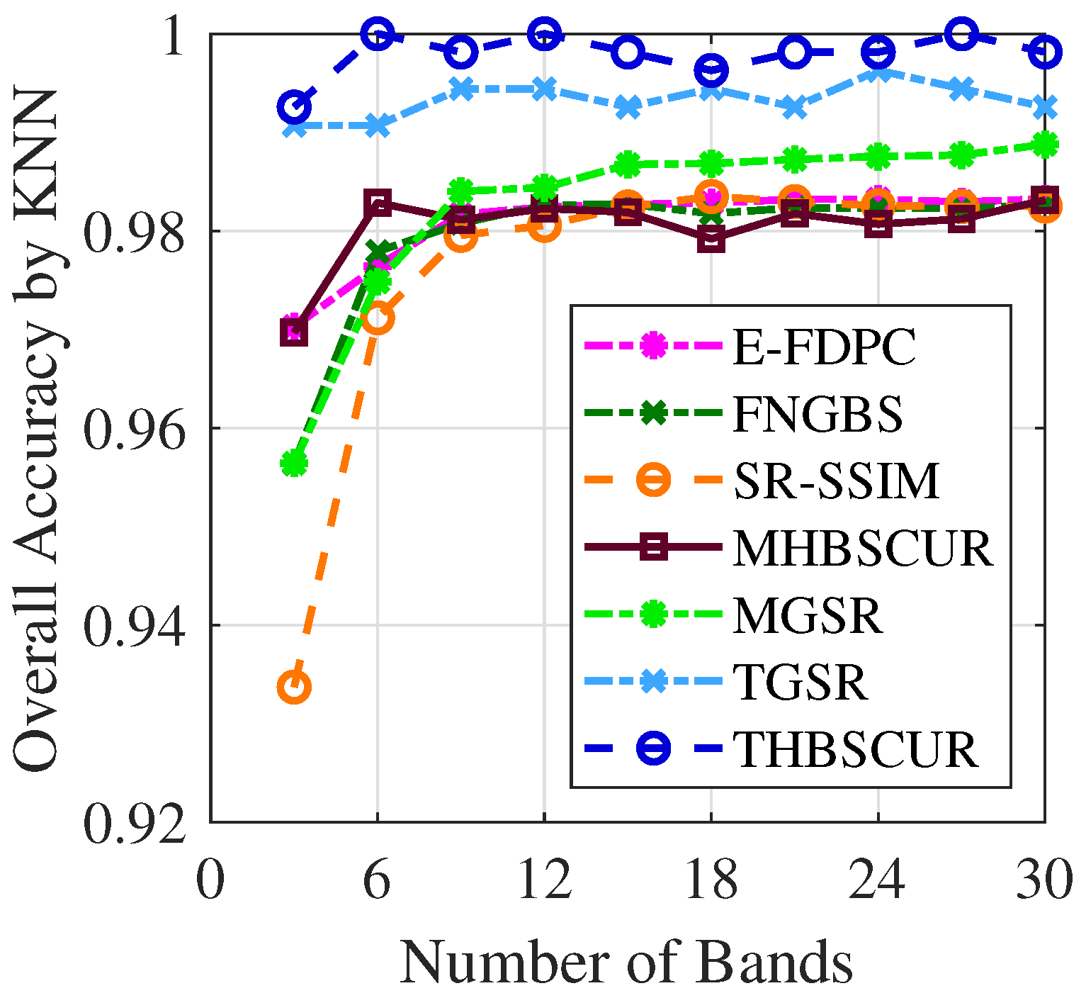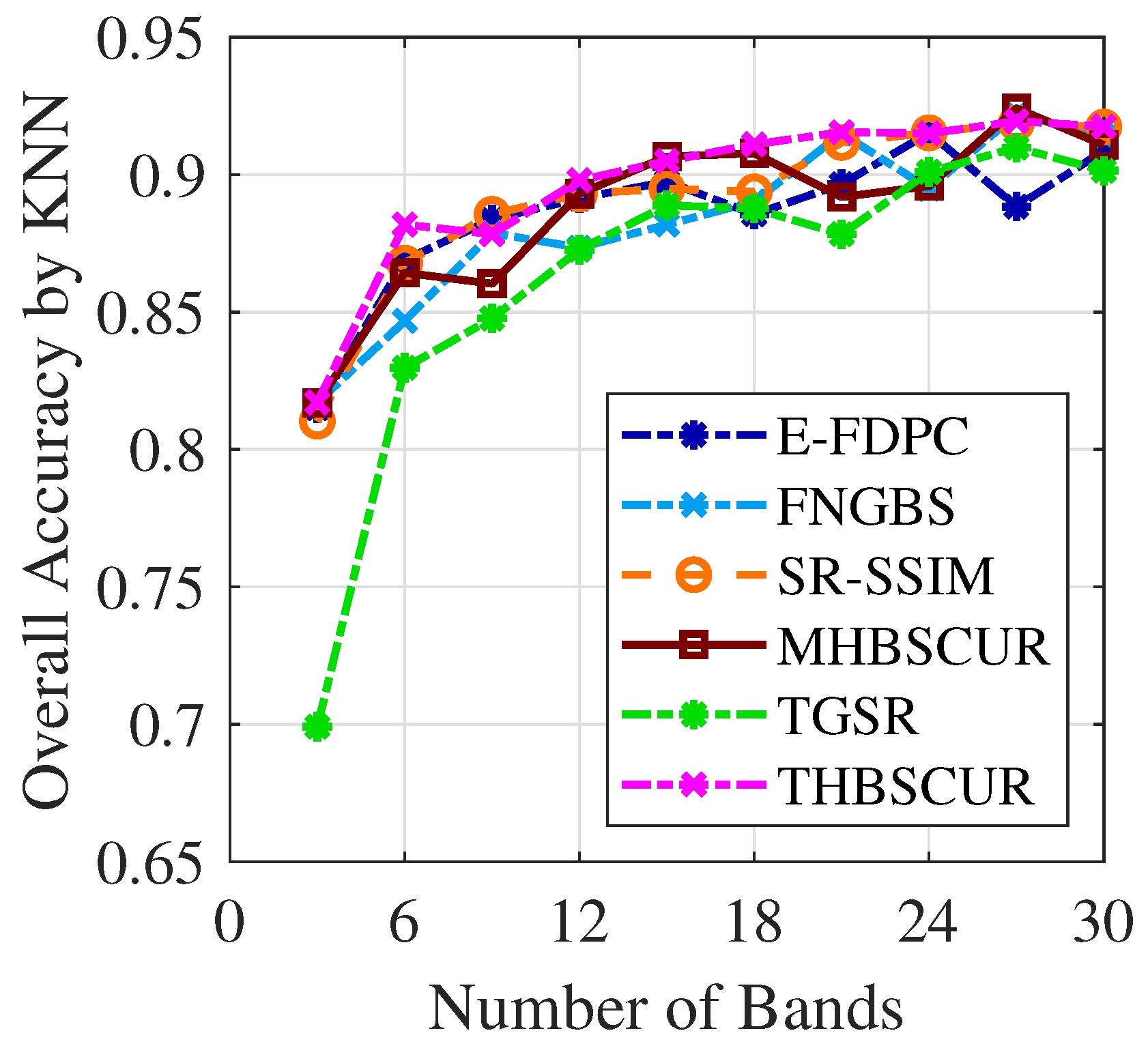Section 4 demonstrates the performance of the proposed method through a series of comprehensive numerical experiments. We evaluate our algorithm using benchmark remote sensing datasets, comparing its performance with state-of-the-art band selection techniques. In Section 5, we discuss parameter selection methods, including grid search and Bayesian Optimization, analyze the impact of noise on the performance of our algorithm, and explore alternative classifiers to demonstrate the robustness of our approach. Finally, conclusions and future work are presented in Section 6.

2. Preliminaries

In this section, we introduce fundamental definitions and notation about third-order tensors [34]. Unless otherwise specified, let $\mathcal{A}\in {\mathbb{R}}^{n_1\times n_2\times n_3}$ and $\mathcal{B}\in {\mathbb{R}}^{n_2\times l\times n_3}$, with the kth frontal slice (or face) of $\mathcal{A}$ denoted by ${\mathcal{A}}_k=\mathcal{A}(:,:,k)$. We also denote the fast Fourier transform of $\mathcal{A}$ along the third dimension as ${\mathcal{A}}_f=\mathtt{f}\mathtt{f}\mathtt{t}(\mathcal{A},\left[\right],3)$ and the inverse FFT of ${\mathcal{A}}_f$ as $\mathtt{i}\mathtt{f}\mathtt{f}\mathtt{t}({\mathcal{A}}_f,\left[\right],3)$. We define the identity tensor $\mathcal{I}$ as the tensor where the first frontal slice is the identity matrix, and all other frontal slices are zeros. Thus, ${\mathcal{I}}_f=\mathtt{f}\mathtt{f}\mathtt{t}(\mathcal{I},\left[\right],3)$ is a tensor where each frontal slice is the identity matrix. The zero tensor is denoted by $\mathcal{O}$. For a finite set I, we use $\left|I\right|$ to denote its cardinality. We also define $\left[n\right]=\{1,2,\dots ,n\}$.

In addition, we define three commonly used tensor norms. The ${\ell }_1$ norm of a tensor $\mathcal{A}$, denoted as ${\left|\right|\mathcal{A}\left|\right|}_1$, is the sum of the absolute values of all its entries. The Frobenius norm of $\mathcal{A}$, denoted as ${\left|\right|\mathcal{A}\left|\right|}_F$, is the square root of the sum of the squared absolute values of all its entries. This norm is analogous to the Frobenius norm for matrices. The ${\ell }_{\infty }$ norm of $\mathcal{A}$, denoted as ${\left|\right|\mathcal{A}\left|\right|}_{\infty }$, is the maximum absolute value among its entries.

Definition 1 

([34]). The block circulant operator, denoted as $\mathit{bcirc}(·)$, converts a tensor to a block circulant matrix and is defined as follows:

$$\mathit{bcirc}\left(\mathcal{A}\right):=\left[\begin{array}{cccc}{\mathcal{A}}_1& {\mathcal{A}}_{n_3}& \cdots & {\mathcal{A}}_2\\ {\mathcal{A}}_2& {\mathcal{A}}_1& \cdots & {\mathcal{A}}_3\\ ⋮& ⋮& \ddots & ⋮\\ {\mathcal{A}}_{n_3}& {\mathcal{A}}_{n_3-1}& \cdots & {\mathcal{A}}_1\end{array}\right]\in {\mathbb{R}}^{n_1{n}_3\times n_2{n}_3}.$$

Definition 2 

([34]). The operator unfold(·) and its inversion fold(·) for the conversion between tensors and matrices are defined as

$$\mathit{unfold}\left(\mathcal{A}\right)=\left[\begin{array}{c}{\mathcal{A}}_1\\ {\mathcal{A}}_2\\ ⋮\\ {\mathcal{A}}_{n_3}\end{array}\right]\in {\mathbb{R}}^{n_1{n}_3\times n_2},\mathit{fold}\left(\left[\begin{array}{c}{\mathcal{A}}_1\\ {\mathcal{A}}_2\\ ⋮\\ {\mathcal{A}}_{n_3}\end{array}\right]\right)=\mathcal{A}.$$

Definition 3 

([34]). The block diagonal matrix form of $\mathcal{A}$, denoted by $\mathit{bdiag}\left(\mathcal{A}\right)$, is defined as a block diagonal matrix with diagonal blocks ${\mathcal{A}}_1,\dots ,{\mathcal{A}}_{n_3}$, i.e.,

$$\mathit{bdiag}\left(\mathcal{A}\right)=\left[\begin{array}{cccc}{\mathcal{A}}_1& & & \\ & {\mathcal{A}}_2& & \\ & & \ddots & \\ & & & {\mathcal{A}}_{n_3}\end{array}\right].$$

Definition 4 

([34]). The t-product of the tensors $\mathcal{A}$ and $\mathcal{B}$ is defined as

$$\mathcal{A}\ast \mathcal{B}:=\mathit{fold}\left(\mathit{bcirc}\right(\mathcal{A}\left)\mathit{unfold}\right(\mathcal{B}\left)\right).$$

The t-product can also be converted to matrix multiplication in the Fourier domain such that $\mathcal{C}=\mathcal{A}\ast \mathcal{B}$ is equivalent to bdiag$\left({\mathcal{C}}_f\right)=\mathit{bdiag}\left({\mathcal{A}}_f\right)\mathit{bdiag}\left({\mathcal{B}}_f\right)$. Note that, given the appropriate dimensions, $\mathcal{A}\ast \mathcal{I}=\mathcal{I}\ast \mathcal{A}=\mathcal{A}$.

Definition 5 

([35]). A tensor $\mathcal{A}\in {\mathbb{R}}^{n\times n\times n_3}$ is orthogonal if ${\mathcal{A}}^{*}\ast \mathcal{A}=\mathcal{A}\ast {\mathcal{A}}^{*}=\mathcal{I}$, for all $i_3\in \left[n_3\right]$, and ${\mathcal{A}}^{*}$ is the complex conjugate transpose of $\mathcal{A}$, which is defined as ${\left({\mathcal{A}}^{*}\right)}_f(:,:,i_3)={\left({\mathcal{A}}_f(:,:,i_3)\right)}^{*}$ for all $i_3\in \left[n_3\right]$.

Definition 6 

([29]). The pseudoinverse (or Moore–Penrose inverse) of the tensor $\mathcal{A}$, denoted by ${\mathcal{A}}^{†}$, is defined by taking the pseudoinverse of each frontal slice in the Fourier domain:

$${\mathcal{A}}^{†}=\mathtt{i}\mathtt{f}\mathtt{f}\mathtt{t}\left(\mathtt{f}\mathtt{o}\mathtt{l}\mathtt{d}\left[\begin{array}{c}{\left({\mathcal{A}}_f\right)}_1^{†}\\ {\left({\mathcal{A}}_f\right)}_2^{†}\\ ⋮\\ {\left({\mathcal{A}}_f\right)}_{n_3}^{†}\end{array}\right],\left[\right],3\right).$$

(1)

Definition 7 

([35]). A tensor $\mathcal{A}$ is f-diagonal if each frontal slice $\mathcal{A}(:,:,i_3)$ is diagonal for all $i_3\in \left[n_3\right]$.

Definition 8 

([35]). The tensor Singular Value Decomposition (t-SVD) induced by the t-product is $\mathcal{A}=\mathcal{U}\ast \mathcal{S}\ast {\mathcal{V}}^{*}$ where $\mathcal{U}\in {\mathbb{R}}^{n_1\times n_1\times n_3}$ and $\mathcal{V}\in {\mathbb{R}}^{n_2\times n_2\times n_3}$ are orthogonal, and the core tensor $\mathcal{S}\in {\mathbb{R}}^{n_1\times n_2\times n_3}$ is f-diagonal. Moreover, the t-SVD rank of tensor $\mathcal{A}$ is defined as ${\mathit{rank}}_t\left(\mathcal{A}\right)=\left|\{i:\mathcal{S}(i,i,1)\ne 0\}\right|$.

Definition 9 

([29]). The multirank of a tensor $\mathcal{A}$ is defined as the vector ${\mathit{rank}}_m\left(\mathcal{A}\right)=(r_1,\dots ,r_{n_3})$, where $r_k=\mathit{rank}\left({\mathcal{A}}_f(:,:,k)\right).$

Definition 10 

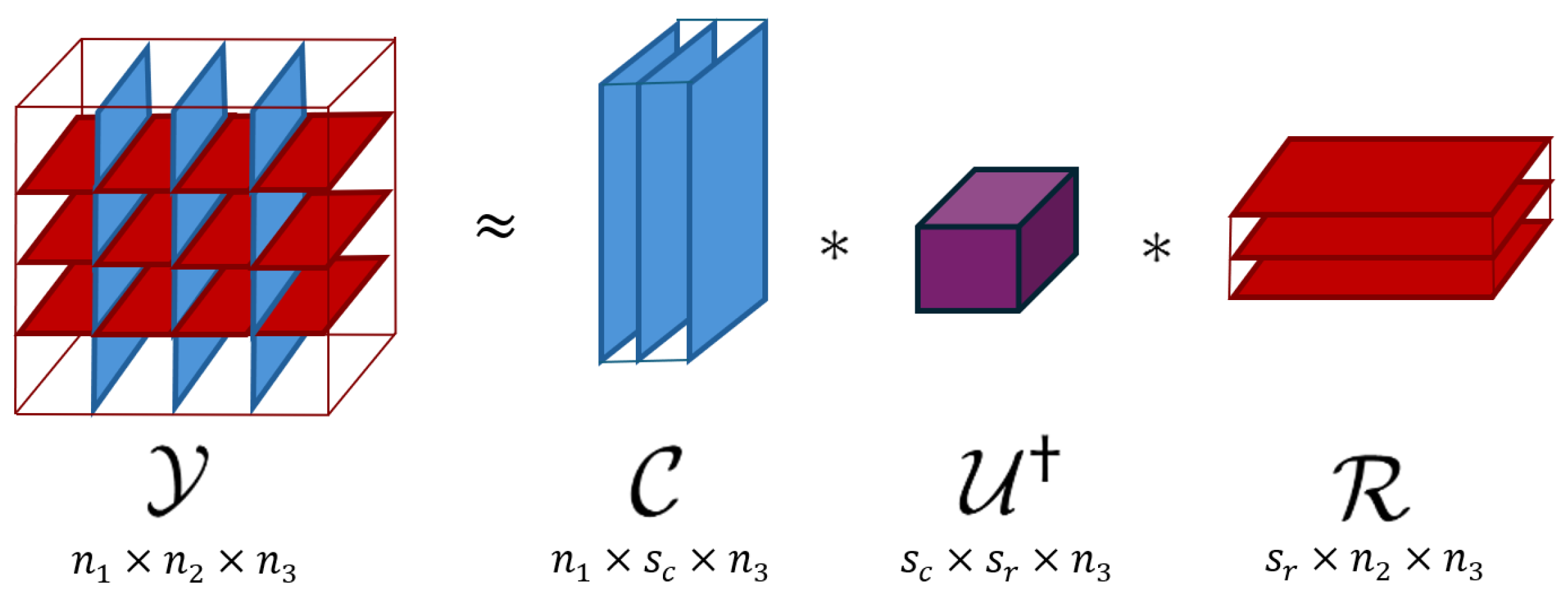
([29]). Consider a tensor $\mathcal{Y}\in {\mathbb{R}}^{n_1\times n_2\times n_3}$. Let $I\subset \{1:n_1\}$ and $J\subset \{1:n_2\}$ be index subsets, and define $\mathcal{R}=\mathcal{Y}(I,:,:)$, $\mathcal{C}=\mathcal{Y}(:,J,:)$, and $\mathcal{U}=\mathcal{Y}(I,J,:)$. The t-CUR decomposition of $\mathcal{Y}$ is $\widehat{\mathcal{Y}}=\mathcal{C}\ast {\mathcal{U}}^{†}\ast \mathcal{R}$, where ${\mathcal{U}}^{†}$ is the pseudoinverse of $\mathcal{U}$ as defined in (1) above. Figure 1 depicts this low-rank decomposition, where $s_r=\left|I\right|$ and $s_c=\left|J\right|$.

Definition 11 

([29]). Consider a tensor $\mathcal{Y}\in {\mathbb{R}}^{n_1\times n_2\times n_3}$ with the multirank ${\mathit{rank}}_m\left(\mathcal{Y}\right)=r_m$ and the t-SVD rank ${\mathit{rank}}_t\left(\mathcal{Y}\right)=r_t$. If the index sets I and J, as defined in the t-CUR decomposition in Definition 10, satisfy $\left|I\right|,\left|J\right|\ge r_t$ and the core tensor $\mathcal{U}$ in the t-CUR decomposition has multirank ${\mathit{rank}}_m\left(\mathcal{U}\right)=r_m$, then the recovery is exact, i.e., $\mathcal{Y}=\widehat{\mathcal{Y}}=\mathcal{C}\ast {\mathcal{U}}^{†}\ast \mathcal{R}$.

Definition 12. 

The proximal operator of ${\ell }_1^p$ is defined as

$$\begin{array}{c}\hfill {prox}_{\lambda {∥·∥}_1^p}\left(\mathcal{Z}\right)=\underset{\mathcal{X}\in {\mathbb{R}}^{n_2\times l\times n_3}}{argmin}{\displaystyle \frac{1}{2}}{\parallel \mathcal{X}-\mathcal{Z}\parallel }_F^2+\lambda {\parallel \mathcal{X}\parallel }_1^p,\end{array}$$

(2)

where $p>0$ is an integer.

Note that the proximal operator ${prox}_{\lambda {∥·∥}_1^p}\left(\mathcal{Z}\right)$ when $p=1,2,3,4$ can be computed using Algorithms 1 and 2 in [36]. If $p=1$, then this is the soft thresholding operator [37].

In addition, to describe smoothness while preserving edge sharpness, the traditional two-dimensional total variation [14] has been extended to 3D images, such as 3DTV [15] and the spatial–spectral total variation for hyperspectral images [16]. Motivated by our recent work on the power of the ${\ell }_1$ norm regularizer [38], we propose a novel generalized 3D total variation regularization to further enhance the sparsity of derivatives.

Definition 13. 

The Generalized 3D Total Variation (G3DTV) regularization of a third-order tensor $\mathcal{U}$ is defined as

$${\parallel \mathcal{U}\parallel }_{\mathrm{G}3\mathrm{DTV}}=\sum _{i=1}^3{\parallel D_i\mathcal{U}\parallel }_1^p$$

(3)

where $p\ge 1$ is an integer, and $D_i$ represents the finite difference operator along the ith mode.

In our experiments, $D_i$ was set as the forward difference operator with Neumann boundary conditions.

3. Proposed Method

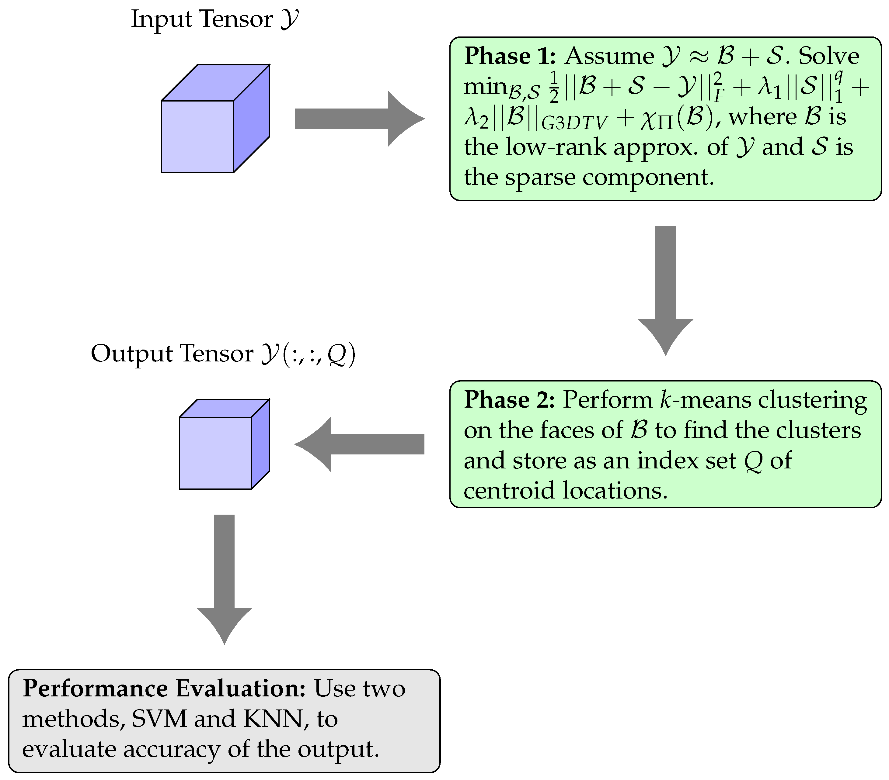
Equipped with the basic knowledge of tensors, we present a novel tensor-based hyperspectral band selection approach, which consists of two phases. In Phase 1, we develop a tensor-based model that decomposes the input tensor $\mathcal{Y}$ into a low-rank and smooth component $\mathcal{B}$ and a sparse component $\mathcal{S}$. In Phase 2, we perform k-means clustering on the frontal slices of $\mathcal{B}$ to identify the most important clusters and store their corresponding centroids in an index set Q. The algorithm then outputs the band-selected tensor $\mathcal{Y}(:,:,Q)$, and we evaluate the accuracy using two data classification methods, i.e., K-Nearest Neighbors (KNNs) and Support Vector Machine (SVM). The entire pipeline is illustrated in Figure 2. It is worth noting that the use of k-means clustering [39] and performance evaluation through classification algorithms are well-established practices in the band selection literature. In what follows, we will dive into the details of Phase 1 of the algorithm, which is the core of our novel contributions.

As depicted in Figure 2, we begin with an initial hyperspectral tensor $\mathcal{Y}\in {\mathbb{R}}^{n_1\times n_2\times n_3}$ with $n_3$ spectral bands, each composed of $n_1\times n_2$ spatial pixels. We introduce an indicator function to take care of the rank constraint. Let $\Pi =\{\mathcal{X}\in {\mathbb{R}}^{n_1\times n_2\times n_3}|{\mathrm{rank}}_{\mathrm{t}}\left(\mathcal{X}\right)\le r\}$. Then, we introduce an indicator function ${\chi }_{\Pi }$ defined as ${\chi }_{\Pi }\left(\mathcal{X}\right)=0$ if $\mathcal{X}\in \Pi$ and as $+\infty$ if otherwise. According to the assumption that the most informative bands are able to preserve spectral relationships and smooth transitions across neighboring bands, we decompose $\mathcal{Y}$ into a sum of a spatial–spectral smooth tensor $\mathcal{B}$, which is low-rank and a sparse tensor $\mathcal{S}$ via the following model:

$$\underset{\mathcal{B},\mathcal{S}}{min}{\displaystyle \frac{1}{2}}{∥\mathcal{B}+\mathcal{S}-\mathcal{Y}∥}_F^2+{\lambda }_1{∥\mathcal{S}∥}_1^q+{\lambda }_2{∥\mathcal{B}∥}_{G3DTV}+{\chi }_{\Pi }\left(\mathcal{B}\right),$$

(4)

where $q\ge 1$ is an integer. The positive parameter ${\lambda }_1$ is the regularization parameter for controlling the sparsity of the outlier tensor $\mathcal{S}$, and ${\lambda }_2>0$ controls the spatial–spectral smoothness of the tensor $\mathcal{B}$. Here, the third term is the G3DTV of $\mathcal{B}$ as defined in Definition 13, i.e., ${∥\mathcal{B}∥}_{G3DTV}={\sum }_{i=1}^3{∥D_i\mathcal{B}∥}_1^p$. The parameter p in the G3DTV and q in the sparsity regularizer are positive integers. Our numerical experiments have shown that $p=2$ and $q=1$ lead to the best performance. In order to apply the ADMM framework to minimize (4), we introduce the auxiliary variables ${\mathcal{X}}_i$ and rewrite (4) as

$$\begin{array}{cc}\hfill \underset{\mathcal{B},\mathcal{S},{\mathcal{X}}_i}{min}& {\displaystyle \frac{1}{2}}{∥\mathcal{B}+\mathcal{S}-\mathcal{Y}∥}_F^2+{\lambda }_1{∥\mathcal{S}∥}_1^q+{\lambda }_2\sum _{i=1}^3{∥{\mathcal{X}}_i∥}_1^p+{\chi }_{\Pi }\left(\mathcal{B}\right)\hfill \\ \hfill & \mathrm{s}.\mathrm{t}.{\mathcal{X}}_i=D_i\mathcal{B}\mathrm{for}i=1,2,3.\hfill \end{array}$$

Then, the augmented Lagrangian reads as

$$\begin{array}{cc}\hfill \mathcal{L}=& {\displaystyle \frac{1}{2}}{∥\mathcal{B}+\mathcal{S}-\mathcal{Y}∥}_F^2+{\lambda }_1{∥\mathcal{S}∥}_1^q+{\chi }_{\Pi }\left(\mathcal{B}\right)+{\lambda }_2\sum _{i=1}^3{∥{\mathcal{X}}_i∥}_1^p+{\displaystyle \frac{\beta }{2}}\sum _{i=1}^3{∥D_i\mathcal{B}-{\mathcal{X}}_i+{\tilde{\mathcal{X}}}_i∥}_F^2.\hfill \end{array}$$

Here, ${\tilde{\mathcal{X}}}_i$ are dual variables, and $\beta >0$ is the penalty parameter. Applying the ADMM algorithm leads to solving three types of subproblems in each iteration. That is, by minimizing $\mathcal{L}$ with respect to $\mathcal{B}$, $\mathcal{S}$, and ${\mathcal{X}}_i$ at each iteration, we obtain the following algorithm:

$$\left\{\begin{array}{cc}\hfill \mathcal{B}\leftarrow & \underset{\mathcal{B}}{argmin}{\displaystyle \frac{1}{2}}{∥\mathcal{B}+\mathcal{S}-\mathcal{Y}∥}_F^2+{\chi }_{\Pi }\left(\mathcal{B}\right)+{\displaystyle \frac{\beta }{2}}\sum _{i=1}^3{∥D_i\mathcal{B}-{\mathcal{X}}_i+{\tilde{\mathcal{X}}}_i∥}_F^2;\hfill \\ \hfill \mathcal{S}\leftarrow & \underset{\mathcal{S}}{argmin}{\displaystyle \frac{1}{2}}{∥\mathcal{B}+\mathcal{S}-\mathcal{Y}∥}_F^2+{\lambda }_1{∥\mathcal{S}∥}_1^q;\hfill \\ \hfill {\mathcal{X}}_i\leftarrow & \underset{{\mathcal{X}}_i}{argmin}{\lambda }_2{∥{\mathcal{X}}_i∥}_1^p+{\displaystyle \frac{\beta }{2}}{∥D_i\mathcal{B}-{\mathcal{X}}_i+{\tilde{\mathcal{X}}}_i∥}_F^2;\hfill \\ \hfill {\tilde{\mathcal{X}}}_i\leftarrow & {\tilde{\mathcal{X}}}_i+D_i\mathcal{B}-{\mathcal{X}}_i.\hfill \end{array}\right.$$

(5)

Here, ${\mathcal{X}}_i$ and ${\tilde{\mathcal{X}}}_i$ are updated for $i=1,2,3$. The $\mathcal{B}$ subproblem is essentially a rank-constrained least-squares problem which has no closed-form solution. Inspired by the fast gradient descent method in robust PCA [27] and its variants [13,28], we employ gradient descent while maintaining the rank constraint. At the jth iteration, we denote the respective estimate of $\mathcal{B},\mathcal{S},{\mathcal{X}}_i$ from the previous iteration by ${\mathcal{B}}^j,{\mathcal{S}}^j,{\mathcal{X}}_i^j$ and then define the objective function f of the $\mathcal{B}$ subproblem without the indicator function as follows:

$$f\left(\mathcal{B}\right):={\displaystyle \frac{1}{2}}{∥\mathcal{B}+{\mathcal{S}}^j-\mathcal{Y}∥}_F^2+{\displaystyle \frac{\beta }{2}}\sum _{i=1}^3{∥{\nabla }_i\mathcal{B}-{\mathcal{X}}_i^j+{\tilde{\mathcal{X}}}_i^j∥}_F^2.$$

Then, $\mathcal{B}$ is updated via ${\mathcal{B}}^{j+1}={argmin}_{{\mathrm{rank}}_t\left(\mathcal{B}\right)\le r}f\left(\mathcal{B}\right).$ To handle the rank constraint, we employ the t-CUR decomposition [29] instead of the skinny t-SVD to reduce computational costs, especially for large tensors. By applying gradient descent with step size $\tau >0$, we obtain the updating scheme for $\mathcal{B}$ as ${\mathcal{B}}^{j+1}={\mathcal{B}}^j-\tau \nabla f\left({\mathcal{B}}^j\right)$, where the gradient is

$$\nabla f\left({\mathcal{B}}^j\right)={\mathcal{B}}^j+{\mathcal{S}}^j-\mathcal{Y}+\beta \sum _{i=1}^3{\nabla }_i^T({\nabla }_i{\mathcal{B}}^j-{\mathcal{X}}_i^j+{\tilde{\mathcal{X}}}_i^j).$$

Then, the factor tensors in the t-CUR decomposition of ${\mathcal{B}}^{j+1}$ are updated as

$$\left\{\begin{array}{cc}\hfill {\mathcal{C}}^{j+1}& ={\mathcal{C}}^j-\tau \nabla f\left({\mathcal{B}}^j\right)(:,J,:),\hfill \\ \hfill {\mathcal{R}}^{j+1}& ={\mathcal{R}}^j-\tau \nabla f\left({\mathcal{B}}^j\right)(I,:,:),\hfill \\ \hfill {\mathcal{U}}^{j+1}& =\frac{1}{2}({\mathcal{C}}^{j+1}+{\mathcal{R}}^{j+1}).\hfill \end{array}\right.$$

(6)

Here, I and J are the respective row and column index sets. Based on the Definition 10, we update $\mathcal{B}$ as

$$\begin{array}{c}\hfill {\mathcal{B}}^{j+1}={\mathcal{C}}^{j+1}\ast {\left({\mathcal{U}}^{j+1}\right)}^{†}\ast {\mathcal{R}}^{j+1}.\end{array}$$

(7)

Both the $\mathcal{S}$ subproblem and the ${\mathcal{X}}_i$ subproblem have closed-form solutions using the proximal operators in the Definition 12. By fixing other variables in the respective $\mathcal{S}$ subproblem and ${\mathcal{X}}_i$ subproblem in (5), we update $\mathcal{S}$ and ${\mathcal{X}}_i$ as

$$\begin{array}{cc}\hfill S^{j+1}& ={prox}_{{\lambda }_1{∥·∥}_1^q}(\mathcal{Y}-{\mathcal{B}}^{j+1}),\hfill \end{array}$$

(8)

$$\begin{array}{cc}\hfill {\mathcal{X}}_i^{j+1}& ={prox}_{{\displaystyle \frac{{\lambda }_2}{\beta }}{∥·∥}_1^p}(D_i{\mathcal{B}}^{j+1}+{\tilde{\mathcal{X}}}_i^j),i=1,2,3.\hfill \end{array}$$

(9)

The algorithm terminates when the convergence condition is met, i.e., the maximum absolute error between two successive solutions falls below a tolerance

$$\parallel {\mathcal{B}}^{j+1}-{\mathcal{B}}^j{\parallel }_{\infty }<\epsilon ,$$

(10)

where $\epsilon$ is a predefined tolerance, e.g., ${10}^{-5}$ for our experiments. While other band selection methods may use a combination of multiple convergence criteria, such as changes in the objective function value or gradient norms, we stick to this single criterion to save computational time and simplify the procedure. Finally, we apply a classifier such as k-means on the frontal slices of $\tilde{\mathcal{B}}$ to find the desired k clusters. The fiber indices of the bands closest to the cluster centroids are stored in the set Q. Thus, the corresponding bands from the original tensor $\mathcal{Y}$ constitute the desired subset of bands.

The main computational cost of Phase 1 in Algorithm 1 is due to the update of $\mathcal{B}$ using the t-product. The per-iteration complexity is $O(n_1{n}_2{n}_{3}log\left(n_3\right)+n_1{s}_r{s}_c{n}_3)$. When $s_c{s}_r\ll n_2$, the term $O(n_1{n}_2{n}_{3}log\left(n_3\right))$ dominates the complexity. This creates a computational trade-off when applying the t-CUR decomposition, as selecting larger values for $s_c$ and $s_r$ leads to increased computational complexity. In Phase 2, the application of k-means clustering requires $O\left(T_k{n}_1{n}_2{n}_{3}k\right)$ operations, provided we have a fixed number of $T_k$ iterations in the k-means clustering. The complexity of this step is directly proportional to the number of selected bands k and the dimensions of the hyperspectral image. Therefore, the overall computational complexity of the algorithm is $O(n_1{n}_2{n}_{3}log\left(n_3\right)+T_k{n}_1{n}_2{n}_{3}k)$.

Algorithm 1 Hyperspectral Band Selection Based on Tensor CUR Decomposition (THBSCUR)

Input: $\mathcal{Y}\in {\mathbb{R}}^{n_1\times n_2\times n_3}$, maximum number of iterations T, number of sampled rows and columns $s_r$ and $s_c$, number of desired bands k, step size $\tau$, parameters ${\lambda }_1,{\lambda }_2,\beta ,$ and tolerance $\epsilon$ Output: The index Q of the desired band set. 1. Optimize the model in (4) using ADMM: Initialize:  ${\mathcal{C}}^0,{\mathcal{U}}^0,{\mathcal{R}}^0,{\mathcal{B}}^0,{\mathcal{S}}^0,{\mathcal{X}}_i^0=\mathcal{O}$ for  $j=0,1,2,3,\dots T-1$  do     Update ${\mathcal{C}}^{j+1},{\mathcal{U}}^{j+1}$, and ${\mathcal{R}}^{j+1}$ as in (6)     Update ${\mathcal{B}}^{j+1}$ as in (7)     Update ${\mathcal{S}}^{j+1}$ by solving (8)     Update ${\mathcal{X}}_i^{j+1}$ by solving ()     Update ${\tilde{\mathcal{X}}}_i^{j+1}={\tilde{\mathcal{X}}}_i^j+D_i{\mathcal{B}}^{j+1}-{\mathcal{X}}_i^{j+1},i=1,2,3$     Check the convergence condition (10)     if converged then         Exit and set $\tilde{\mathcal{B}}={\mathcal{B}}^{j+1}$     end if end for Set $\tilde{\mathcal{B}}={\mathcal{B}}^{T+1}$ 2. Cluster frontal slices of $\tilde{\mathcal{B}}$ using a clustering method such as k-means or spectral clustering to find the index set Q which indicates the bands closest to the k cluster centroids.

4. Experimental Data and Results

4.1. Experimental Setup

In our numerical experiments, we evaluated the proposed method using three publicly available HSI datasets visualized in Figure 3: Indian Pines, Salinas-A, and Pavia University (The data are publicly available at the following link: https://www.ehu.eus/ccwintco/index.php/Hyperspectral_Remote_Sensing_Scenes, accessed on 18 December 2024). To assess the effectiveness of our approach, we compared it with several other state-of-the-art band selection methods, including E-FDPC [6], SR-SSIM [9], FNGBS [8], MGSR [10], MHBSCUR [13], and TGSR [11]. The memory complexity of the TGSR algorithm is $O(V{n}_1^2{n}_2^2+V{n}_1{n}_2{n}_3+n_3^2)$, where V refers to the number of unique superpixel regions. This reflects the dependence of the algorithm on both spatial dimensions and spectral bands, with a significant contribution from the quadratic scaling of pixel interactions in each superpixel region. In contrast, the proposed THBSCUR algorithm has a complexity of $O(n_1{n}_2{n}_3+r_s{c}_s{n}_3+k{n}_1{n}_2)$, which simplifies to $O\left(n_1{n}_2{n}_3\right)$ when considering the dominant factor of tensor dimensions. The memory complexity of MHBSCUR is $O(n_1{n}_2{n}_3+n_3^2+n_1^2{n}_2^2)$, where the Laplacian graph computation dominates the complexity, but efficient data structures reduce the practical memory usage. The MGSR algorithm has a memory complexity of $O(n_1^2{n}_2^2+n_3^2+n_1{n}_2{n}_3)$, highlighting its quadratic scaling in the spatial dimensions and its dependence on both the spectral and spatial features. E-FDPC and FNGBS both exhibit a simpler memory complexity of $O\left(n_3^2\right)$, indicating that their performance is more dependent on the spectral dimension. Similarly, the complexity of the SR-SSIM algorithm, $O(n_3^2+n_1{n}_2{n}_3)$, is influenced by both spectral and spatial features, with the spectral component dominating.

For Algorithm 1, the selection of specific rows and columns was randomly selected at the beginning of each trial and then fixed throughout the algorithm. This selection was implemented using a random permutation, where the Mersenne Twister generator seed [40] was initialized to 1 at the start of each trial. For each dataset, classification approach, and targeted number of bands, we fine-tuned the parameters ${\lambda }_1,{\lambda }_2$, $\beta$, and $\tau$ using Bayesian Optimization (BO). Refer to Section 5 for further discussion on parameter tuning.

We evaluated the performance of these methods through classification tests using SVM and KNN, measuring their effectiveness with the Overall Accuracy (OA) metric, which is defined as the ratio of correctly classified samples to the total number of samples in the test set. For the classification setup, we randomly selected 90% of the samples from each dataset for training and the remaining 10% for testing. To reduce the randomness effect, each classification test was repeated 50 times with different training data. The number of bands tested ranged from 3 to 30, increasing in increments of three.

All numerical experiments were conducted using MATLAB 2023b on a desktop computer equipped with an Intel i7-1065G7 CPU, 12GB RAM, and running Windows 11.

4.2. Experiment 1: Indian Pines

In the first experiment, we tested the Indian Pines dataset, acquired by the Airborne Visible InfraRed Imaging Spectrometer (AVIRIS) sensor in Northwestern Indiana, which contains $145\times 145$ pixels, 200 spectral bands, and 16 distinct classes. Figure 4 and Figure 5 plot the OA curves produced by SVM and KNNs, respectively, for this dataset. In general, as the number of selected bands increased, the overall accuracy for all methods plateaued. The proposed THBSCUR outperformed the state-of-the-art methods in terms of its OA when SVM or KNNs was used to classify the results for a high number of bands. In this case, SVM also produced slightly higher classification accuracy than KNNs. The average running times for each method in seconds averaged over the number of selected bands k are $0.0382$ for E-FDPC, $0.1417$ for FNGBS, $30.1334$ for SR-SSIM, $15.3760$ for MHBSCUR, $19.7766$ for MGSR, $32.2180$ for TGSR, and $169.5353$ for the proposed method. One can see that while our method required a longer running time, our BO-optimized THBSCUR algorithm achieved comparable or superior classification accuracy across different datasets and classifiers. The consistent improvement in performance observed with our method, especially when considering the optimization across various numbers of selected bands, highlights its robustness and effectiveness. This competitive edge against state-of-the-art methods like TGSR further validates the significance of our approach.

4.3. Experiment 2: Salinas-A

In the second experiment, we tested the Salinas-A dataset, which is a subset of a larger image captured by the AVIRIS sensor in California, consisting of $86\times 83$ pixels, 204 bands, and six classes. Figure 6 and Figure 7 plot the OA curves produced by SVM and KNNs, respectively, for the Salinas-A dataset. The average running times for each method in seconds averaged over the number of selected bands k are $0.0107$ for E-FDPC, $0.0502$ for FNGBS, $22.673$ for SR-SSIM, $6.1636$ for MHBSCUR, $5.9491$ for MGSR, $39.2225$ for TGSR, and $75.1455$ for the proposed method. Despite a longer running time, the proposed method exhibited consistently superior performance with both the SVM and KNNs classifiers.

4.4. Experiment 3: Pavia University

In the third experiment, we evaluated the Pavia University dataset, which was acquired by the Reflective Optics System Imaging Spectrometer (ROSIS) sensor over the urban area of Pavia, Italy. This dataset consists of $610\times 340$ pixels with 103 spectral bands. The Pavia University scene is characterized by its complex urban environment, featuring nine distinct land-cover classes. This dataset is particularly challenging due to its urban complexity and the spectral similarity between some of the classes, such as asphalt and bitumen. The high spatial resolution combined with the diverse urban classes makes Pavia University a valuable benchmark for evaluating hyperspectral image classification algorithms in urban environments.

Figure 8 and Figure 9 plot the OA curves produced by SVM and KNNs, respectively. The average running times for each method in seconds averaged over the number of selected bands k are $0.2537$ for E-FDPC, $0.9218$ for FNGBS, $138.8463$ for SR-SSIM, $3.3029\times {10}^3$ for MHBSCUR, $56.0402$ for TGSR, and $654.5938$ for the proposed method. Overall, THBSCUR performed comparably or outperformed the other methods, especially when the number of selected bands was low. The MGSR method was excluded here due to computational limitations. Specifically, the construction of the adjacency matrix during the preprocessing stage of MGSR led to an out-of-memory error, making it infeasible for this experiment. Meanwhile, this highlights the computational challenges that can arise when dealing with large, high-dimensional hyperspectral datasets.

5. Discussion

In this section, we discuss key aspects of the proposed THBSCUR algorithm that may impact its performance in hyperspectral band selection. We begin by providing detailed guidance on parameter selection using both a traditional grid search method and Bayesian Optimization. We offer insights into optimal parameter ranges for different datasets and discuss the impact of noise on these choices. Then we show the performance of our algorithm in the noisy setting, providing recommendations for parameter adjustments. Finally, we extend our analysis to include additional classifiers, such as the convolutional neural network (CNN) [41], to further validate the effectiveness of our method across different classification approaches in calculating overall accuracy. Throughout this discussion, we aim to provide a comprehensive understanding of the proposed algorithm, practical implementation considerations, and the robustness across various scenarios and classification techniques.

5.1. Parameter Selection via Bayesian Optimization

In the previous sections, we presented the numerical experiment results for the proposed THBSCUR method, which were obtained using Bayesian Optimization [42] for parameter tuning. In this section, we will delve deeper into the details of this optimization process and compare it to the exhaustive grid search commonly used in practice.

Bayesian Optimization-based parameter selection is a powerful and efficient strategy for tuning parameters in unsupervised algorithms. It is particularly useful in machine learning, where the objective function can be the performance of a model, such as loss or accuracy, and the parameters to be optimized may include regularization coefficients and learning rates. Unlike a grid search which evaluates the objective function exhaustively, Bayesian Optimization uses a probabilistic model and acquisition function to explore the parameter space by prioritizing the most promising regions based on prior evaluations, often leading to faster convergence.

In our approach, the parameters to be optimized are $\beta ,{\lambda }_1,{\lambda }_2,$ and $\tau$, which are critical to the performance of THBSCUR. Next, we consider a Bayesian Optimization problem that maximizes the overall classification accuracy of the THBSCUR-based feature selection on hyperspectral data. That is, we solve the following problem:

$$\{{\beta }^{*},{\lambda }_1^{*},{\lambda }_2^{*},{\tau }^{*}\}=\underset{(\beta ,{\lambda }_1,{\lambda }_2,\tau )\in \Gamma }{argmax}\mathrm{OA}(\beta ,{\lambda }_1,{\lambda }_2,\tau ,k),$$

where the parameter space $\Gamma =[a,b]\times [c,d]\times [e,f]\times [g,h]$ (refer to Section 5.2 for more details), k represents the number of spectral bands selected, and OA is defined in Section 4.1. Since there is no analytical expression for the objective function, a probabilistic surrogate model is used to approximate the unknown OA for various combinations of parameters. The surrogate model is a Gaussian Process (GP), which is fully specified by a mean function and a covariance function. The GP model captures both the estimated value of the objective function, which in this case is the overall accuracy, and the uncertainty around this estimate.

The next step in Bayesian Optimization involves strategically selecting the next set of parameters to evaluate. This is accomplished by minimizing an acquisition function, which balances the exploration of uncertain areas with the exploitation of promising regions. Common choices for the acquisition function include the Expected Improvement (EI), Probability of Improvement (PI), and Lower Confidence Bound (LCB).

In our experiments, we used the “bayesopt” function in MATLAB to implement Bayesian Optimization and adopted the “expected-improvement-plus” acquisition function, which is an enhanced version of the EI to prevent the overexploitation of some areas.

5.2. Optimal Parameters for Grid Search and Bayesian Optimization

In this section, we discuss optimal parameters for each test dataset using grid search and Bayesian Optimization, along with general guidelines. Before delving into specific tuning processes, it is important to understand the key parameters in the tensor CUR decomposition that influence the performance of our band selection method.

In the tensor CUR decomposition, the numbers of selected rows and columns, denoted as $s_c$ and $s_r$, are key factors influencing both approximation quality and computational efficiency. There are a few common approaches to determining these parameters. One simple approach is to choose a target rank k, i.e., the number of bands, for the approximation. Another approach, which we adopt here, is to choose $s_c$ and $s_r$ as small multiples of k as $O(klog\left(n_1{n}_2\right))$ and $O(klog\left(n_2\right))$, respectively [43]. Throughout our experiments, we set $s_c$ and $s_r$ to $\mathrm{round}(klog\left(n_1{n}_2\right))$ and $\mathrm{round}(klog\left(n_2\right))$, respectively. The logarithmic factor provides a slight oversampling beyond the rank k, which helps to ensure that enough information is captured to accurately represent the k-dimensional subspace of the data. This oversampling accounts for potential noise or minor variations in the data that might not be captured by selecting exactly k columns and rows.

For the THBSCUR algorithm, we compared two methods of parameter tuning for the parameters ${\lambda }_1$, ${\lambda }_2$, $\beta$, and $\tau$: grid search and BO. The ranges for the grid search approach were defined as follows:

• ${\lambda }_1$, ${\lambda }_2\in \{{10}^{-4},{10}^{-3},{10}^{-2},{10}^{-1},1,10,{10}^2,{10}^3\}$;
• $\beta$, $\tau \in \{{10}^{-1},1,10,{10}^2\}$.

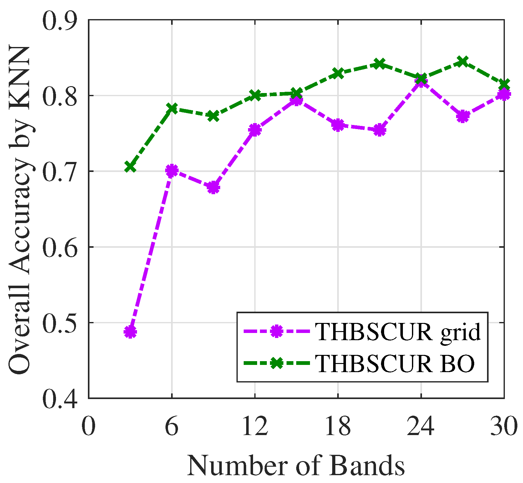
As the number of selected bands increases, the optimal choices for ${\lambda }_1$ and ${\lambda }_2$ become stable, while $\beta$ and $\tau$ require more careful tuning. We suggest starting with $\beta$ and $\tau$ set to 1 and then fine-tuning based on the specific dataset. Importantly, there exist multiple combinations of parameter choices that may lead to optimal overall accuracy. It is worth noting that the optimal parameters found through grid search may differ from those identified using Bayesian Optimization, as the latter explores the parameter space more efficiently and can potentially discover better combinations.

The optimal parameters for the SVM classifier on the Indian Pines dataset, obtained by grid search and presented in

Table 1. Optimal SVM grid search parameters for Indian Pines with different k bands, including the mean and Standard Deviation (SD).

k	$\mathit{\beta }$	${\mathit{\lambda }}_1$	${\mathit{\lambda }}_2$	$\mathit{\tau }$
3	1	$1.0\times {10}^{-4}$	$1.0\times {10}^{-4}$	1
6	10	$1.0\times {10}^{-4}$	$1.0\times {10}^{-4}$	0.1
9	100	$1.0\times {10}^{-4}$	$1.0\times {10}^{-4}$	0.1
12	1	$1.0\times {10}^{-4}$	$1.0\times {10}^{-4}$	10
15	1	$1.0\times {10}^{-4}$	$1.0\times {10}^{-4}$	10
18	10	$1.0\times {10}^{-4}$	$1.0\times {10}^{-3}$	0.1
21	100	$1.0\times {10}^{-4}$	$1.0\times {10}^{-4}$	1
24	1	$1.0\times {10}^{-4}$	$1.0\times {10}^{-4}$	1
27	1	$1.0\times {10}^{-4}$	$1.0\times {10}^{-4}$	10
30	1	$1.0\times {10}^{-4}$	$1.0\times {10}^{-1}$	0.1
Mean	32.4000	$1.0\times {10}^{-4}$	$1.1\times {10}^{-2}$	3.3400
SD	40.9585	0	$3.1561\times {10}^{-2}$	4.6126

, reveal distinct patterns across different numbers of selected bands. The parameter $\beta$ demonstrated the highest variability, with a Standard Deviation (SD) of $40.9585$, indicating that the algorithm is particularly sensitive to the number of selected bands.

The parameter ${\lambda }_1$ remained constant at $0.0001$ for all k values, indicating that the sparsity control for one aspect of the decomposition is consistent across different band selection scenarios. In contrast, ${\lambda }_2$ showed some variation, with a standard deviation of $3.1561\times {10}^{-2}$, primarily due to a single outlier value of $0.1$ at $k=30$. The parameter $\tau$, which governs the step size in the $\mathcal{B}$ update, displayed considerable variability with a standard deviation of $4.6126$, taking on values of $0.1$, 1, and 10 across different k values.

These results indicate that grid search can identify discrete, widely spaced optimal values for $\beta$ and $\tau$ while maintaining more consistent values for ${\lambda }_1$ and ${\lambda }_2$ (with one exception). This discretization is a characteristic of the grid search method, which may miss the fine-grained optimal parameter values that could exist between the tested grid points. The high variability in $\beta$ and $\tau$ highlights the need of careful parameter tuning in the THBSCUR algorithm for different band selection scenarios.

To allow for a more refined exploration of the parameter space, we additionally employed BO to further refine the parameter selection process for the THBSCUR algorithm. In our implementation, the ranges for the four optimizable variables were defined as follows:

• $\beta ,\tau \in [0.1,10]$;
• ${\lambda }_1,{\lambda }_2\in [{10}^{-4},0.01]$.

These ranges were chosen based on insights gained from the initial grid search on the THBSCUR algorithm. The Bayesian Optimization approach complements grid search by providing a more refined exploration of the parameter space, uncovering optimal parameter combinations that were missed in the discrete grid search. For implementation details, refer to Section 5.1.

The optimal parameters for the SVM classifier on the Indian Pines dataset, as shown in

Table 2. Optimal SVM BO parameters of our algorithm for the Indian Pines dataset with different k bands, including the mean and Standard Deviation (SD).

k	$\mathit{\beta }$	${\mathit{\lambda }}_1$	${\mathit{\lambda }}_2$	$\mathit{\tau }$
3	2.9918	$5.4\times {10}^{-3}$	$1.7\times {10}^{-3}$	9.7053
6	9.624	$9.4\times {10}^{-3}$	$2.5\times {10}^{-3}$	0.1224
9	0.1192	$9.9\times {10}^{-3}$	$6.8\times {10}^{-3}$	5.0883
12	0.1247	$3.2\times {10}^{-4}$	$1.3\times {10}^{-4}$	0.1345
15	0.1077	$2.0\times {10}^{-3}$	$8.0\times {10}^{-3}$	1.0986
18	9.913	$8.4\times {10}^{-3}$	$7.0\times {10}^{-3}$	0.7634
21	1.5704	$4.2\times {10}^{-3}$	$1.7\times {10}^{-3}$	0.1980
24	3.422	$4.7\times {10}^{-3}$	$3.4\times {10}^{-3}$	6.4772
27	0.2138	$1.0\times {10}^{-4}$	$8.4\times {10}^{-4}$	8.7834
30	0.1398	$1.7\times {10}^{-3}$	$3.2\times {10}^{-3}$	0.1031
Mean	2.8226	$4.6\times {10}^{-3}$	$3.5\times {10}^{-3}$	3.2474
SD	3.8651	$3.7\times {10}^{-3}$	$2.8\times {10}^{-3}$	3.8816

, reveal interesting patterns across different numbers of selected bands. The parameter $\beta$ exhibited the highest variability, with a standard deviation of $3.8651$. The parameters ${\lambda }_1$ and ${\lambda }_2$, which control the sparsity of the decomposition, showed relatively consistent values across different k, with means of $4.6\times {10}^{-3}$ and $3.5\times {10}^{-3}$, respectively. The parameter $\tau$, governing the threshold in the iterative process, also displayed high variability with a standard deviation of $3.8816$. This variability in $\beta$ and $\tau$ indicates that these parameters are particularly sensitive to the number of selected bands, while the sparsity-controlling parameters ${\lambda }_1$ and ${\lambda }_2$ remain more stable.

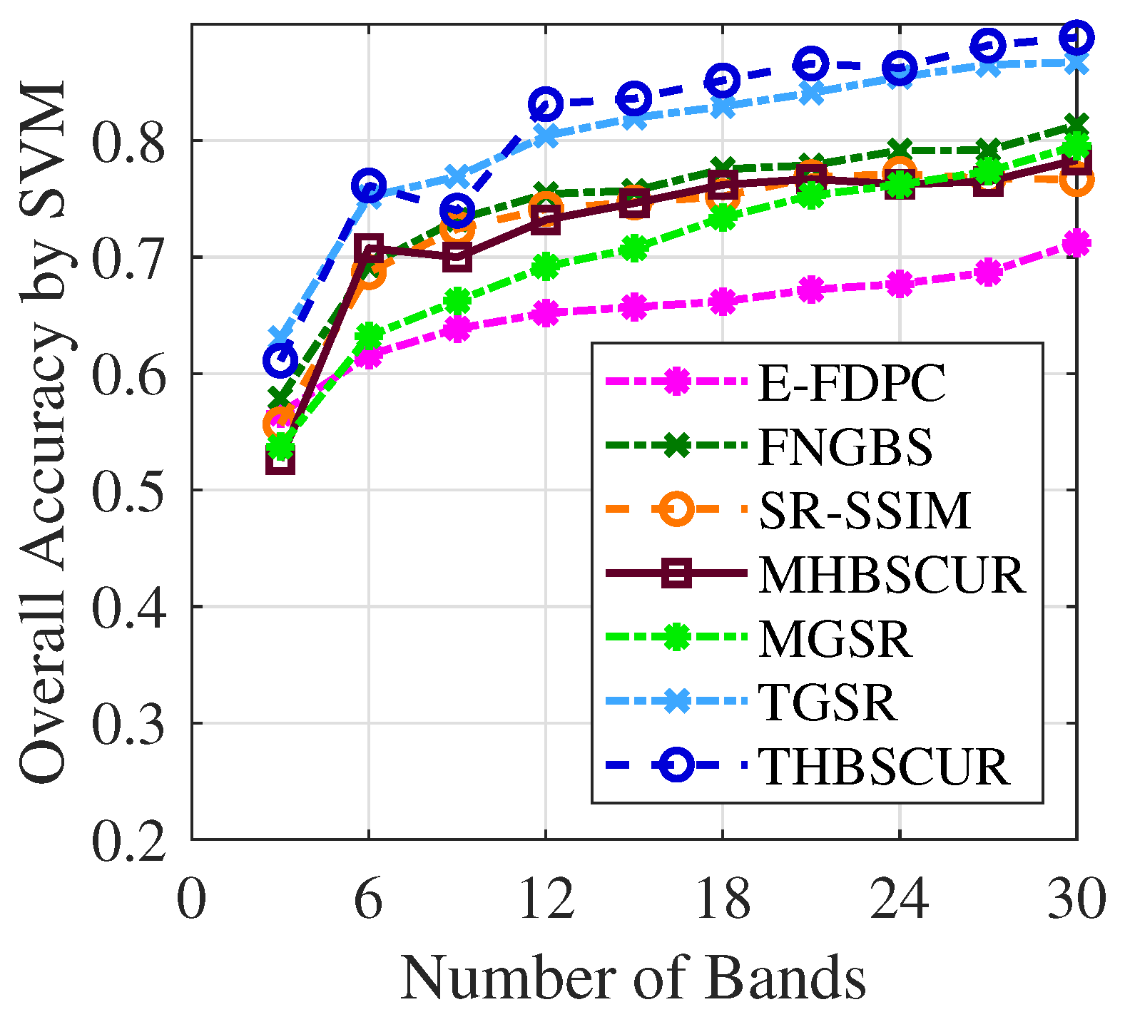
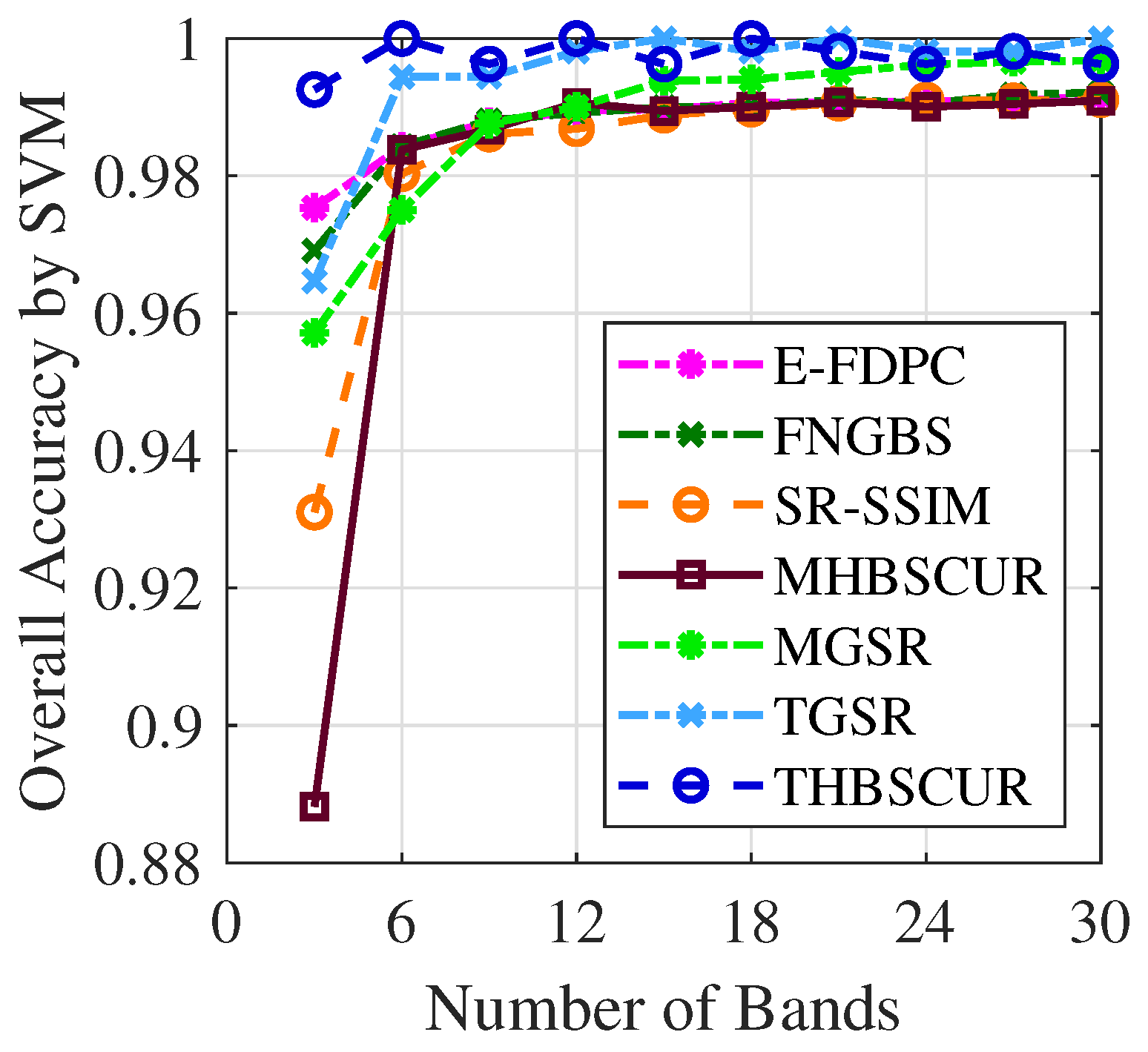
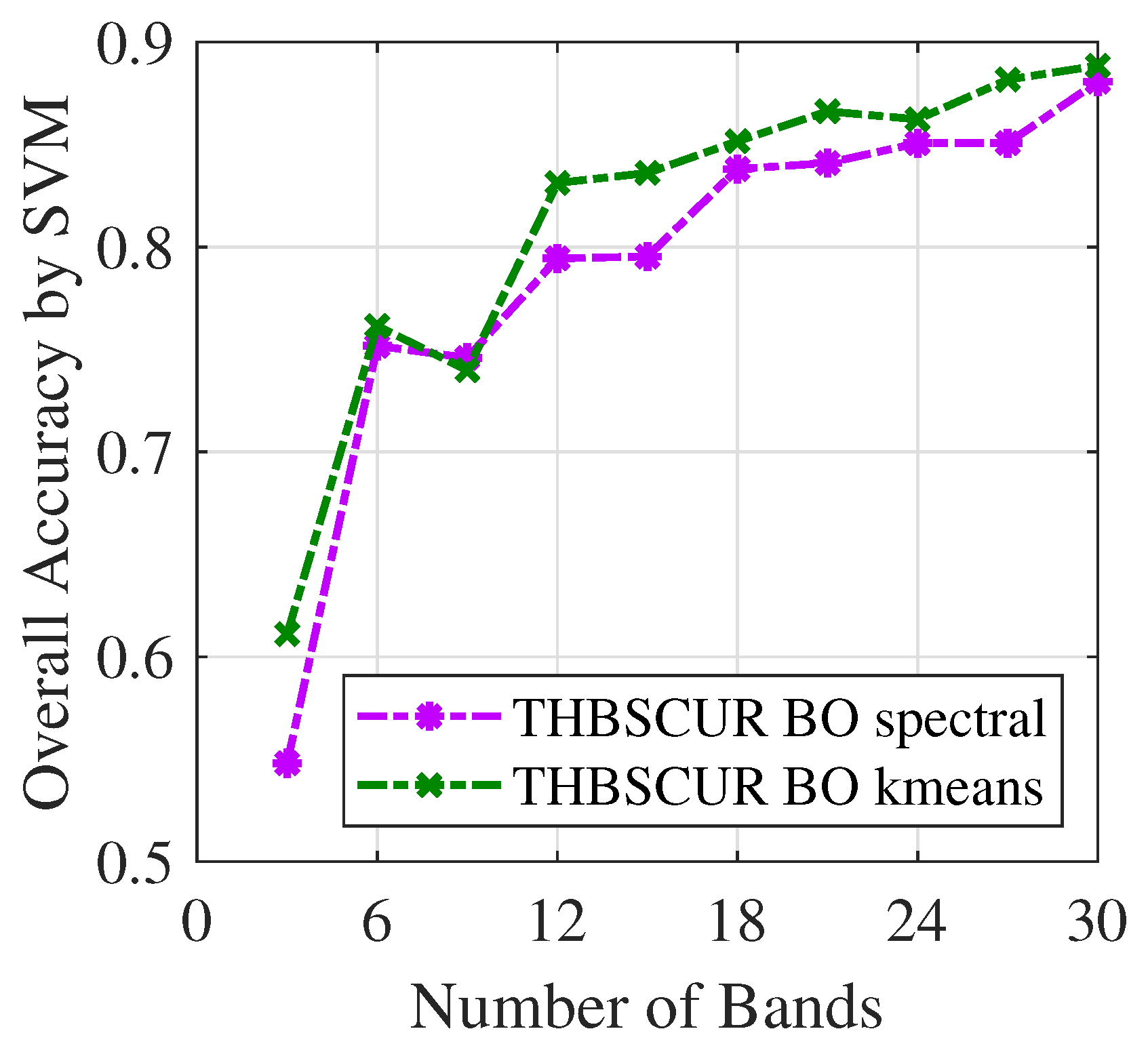
Figure 10 and Figure 11 demonstrate the success of the BO results with the THBSCUR algorithm applied to the Indian Pines dataset. The graphs show a consistent improvement in the classification accuracy across all numbers of selected bands when compared to grid search. This improvement is evident for both the SVM and KNNs classifiers, with BO-optimized parameters yielding higher accuracy levels regardless of the number of bands selected. This consistent superiority of the BO-tuned method underscores its effectiveness in fine-tuning the THBSCUR algorithm parameters, leading to more robust and accurate hyperspectral band selection across various scenarios.

5.3. Effects of Noise

In addition to the optimal parameter ranges outlined in Table 1 and Table 2, it is important to consider the effects of noise on parameter selection for THBSCUR. Hyperspectral data are often polluted by noise, commonly modeled as Gaussian noise, which can significantly impact the performance of band selection algorithms. To address this, we applied parameter adjustments to accommodate the deviations from the original signal introduced by the noise.

In scenarios where Gaussian noise with varying standard deviation levels is introduced into the dataset, we propose the following guidelines for selecting 15 bands from the Indian Pines dataset. The parameters ${\lambda }_1$ and ${\lambda }_2$, which control the trade-off between the sparsity term and the G3DTV regularization term, may require adjustment to mitigate the effects of noise. For noisy cases, $\beta =1$ and $\tau ={10}^{-4}$ consistently yield optimal results across different noise levels. Notably, for each noise level, multiple combinations of ${\lambda }_1$ and ${\lambda }_2$ can lead to optimal outcomes. Tuning ${\lambda }_2$ is particularly critical, as optimal results can still be achieved with varying ${\lambda }_1$ values. The optimal parameters for $\sigma =1,2,3,4,5,6$ are presented in

Table 3. Optimal parameters of our algorithm for Indian Pines with Gaussian noise.

Parameters	$\mathit{\sigma }=1$	$\mathit{\sigma }=2$	$\mathit{\sigma }=3$	$\mathit{\sigma }=4$	$\mathit{\sigma }=5$	$\mathit{\sigma }=6$
${\lambda }_1$	${10}^{-3}$	${10}^{-3}$	${10}^{-3}$	${10}^{-3}$	${10}^{-3}$	${10}^{-1}$
${\lambda }_2$	10	10	${10}^{-2}$	${10}^{-2}$	${10}^{-3}$	${10}^{-2}$
$\beta$	1	1	1	1	1	1
$\tau$	${10}^{-4}$	${10}^{-4}$	${10}^{-4}$	${10}^{-4}$	${10}^{-4}$	${10}^{-4}$

.

5.4. Method Selection for Phase 2

In Phase 2 of our algorithms, we applied the k-means clustering to group the spectral bands and ultimately generate a final index set of k representative bands. This process begins with the refined band representation $\tilde{\mathcal{B}}$ obtained in the previous phase and treating each frontal slice of $\tilde{\mathcal{B}}$ as a data point for further classification. The k-means algorithm begins by randomly choosing k cluster centers from the band data. Each band is then assigned to the nearest cluster center, and the cluster centers are updated as the mean of all bands assigned to each cluster. This iterative process continues until convergence, resulting in a set of representative bands that capture the representative information from the original spectral data. By default, the k-means algorithm in MATLAB uses Euclidean distance. However, we opted to use Manhattan distance instead, as the Euclidean distance-based approach may fail to converge in our experiments. This modification significantly improved the robustness and stability of the clustering process, particularly because the Manhattan distance is more robust in the presence of outliers [44,45].

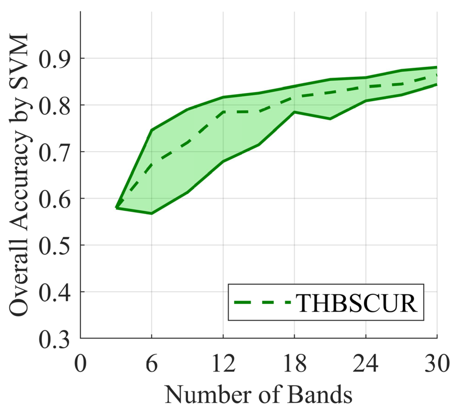
To evaluate the stability and robustness of the k-means clustering process, we conducted 50 trials with random centroid initializations and visualized the results using an envelope plot in Figure 12. This plot highlights the variability in performance by displaying the maximum, minimum, and mean SVM accuracies across all trials for the Indian Pines dataset. The shaded region between the max and min values represents the range of possible outcomes, while a dashed line indicates the mean accuracy. In our experiments, the envelope plot consistently demonstrated a narrow band, signifying minimal variation across trials and showcasing the stability of our k-means-based band selection.

While k-means is effective for hyperspectral band selection, there are several alternative clustering methods that could be considered for band selection. One advantage of k-means is its relative high speed, making it an efficient choice for clustering in this context; alternative methods may not offer the same level of computational efficiency. To explore the effectiveness of other clustering approaches, we implemented and tested three additional methods: spectral clustering, fuzzy c-means [46], and Density-based Spatial Clustering of Applications with Noise (DBSCAN) [47] using MATLAB implementations.

Table 4. Computational time complexity for various methods for Phase 2 of the algorithm for data of size $n_1\times n_2\times n_3$. Here, $T_k$ denotes the number of iterations, and k is the number of classes.

Method	Time Complexity
k-means	$O\left(T_k{n}_1{n}_2{n}_{3}k\right)$
spectral clustering	$O\left({\left(n_1{n}_2{n}_3\right)}^3\right)$
DBSCAN	$O\left({\left(n_1{n}_2{n}_3\right)}^2\right)$
fuzzy c-means	$O\left(T_k{n}_1{n}_2{n}_{3}k\right)$

details the computational complexity of the methods mentioned in this section.

We first implemented spectral clustering using the “spectralcluster” function in MATLAB, which leverages graph-based techniques to partition the spectral bands. Spectral clustering transforms the data into a lower-dimensional space using the eigenvalues of a similarity matrix, capturing complex relationships between bands that may not be evident in the original high-dimensional space. When applied to hyperspectral band selection, spectral clustering produced comparable results compared to the k-means approach. Figure 13 demonstrates the performance of the spectral clustering method as opposed to the k-means method for the Indian Pines dataset.

The fuzzy c-means algorithm, which allows for soft cluster assignments, showed moderate performance. With optimized parameters, it achieved an overall accuracy of 0.6 for the Indian Pines dataset using an SVM classifier to assess the performance. This result, while not surpassing our k-means approach, demonstrates that fuzzy clustering could be a viable alternative for hyperspectral band selection.

In contrast, the DBSCAN algorithm struggled to perform well in this context. Despite its ability to discover clusters, DBSCAN only averaged about 0.2 for overall accuracy across our experiments. This poor performance can be attributed to several factors, including the high-dimensional nature of hyperspectral data and the sensitivity of the algorithm to its input parameters (epsilon and minimum points). The density-based approach of DBSCAN may not be well suited to the spectral characteristics of hyperspectral bands, where the concept of density in high-dimensional space becomes less intuitive.

These results underscore the effectiveness of our k-means-based approach for hyperspectral band selection. While fuzzy c-means shows potential with moderate performance, and spectral clustering demonstrates competitive results, the significant underperformance of DBSCAN highlights the challenges of applying density-based clustering to this specific problem domain. Our findings suggest that centroid-based clustering methods such as k-means and fuzzy c-means, along with graph-based clustering methods like spectral clustering, are well suited for hyperspectral band selection tasks.

5.5. Classifier Selection for Evaluation

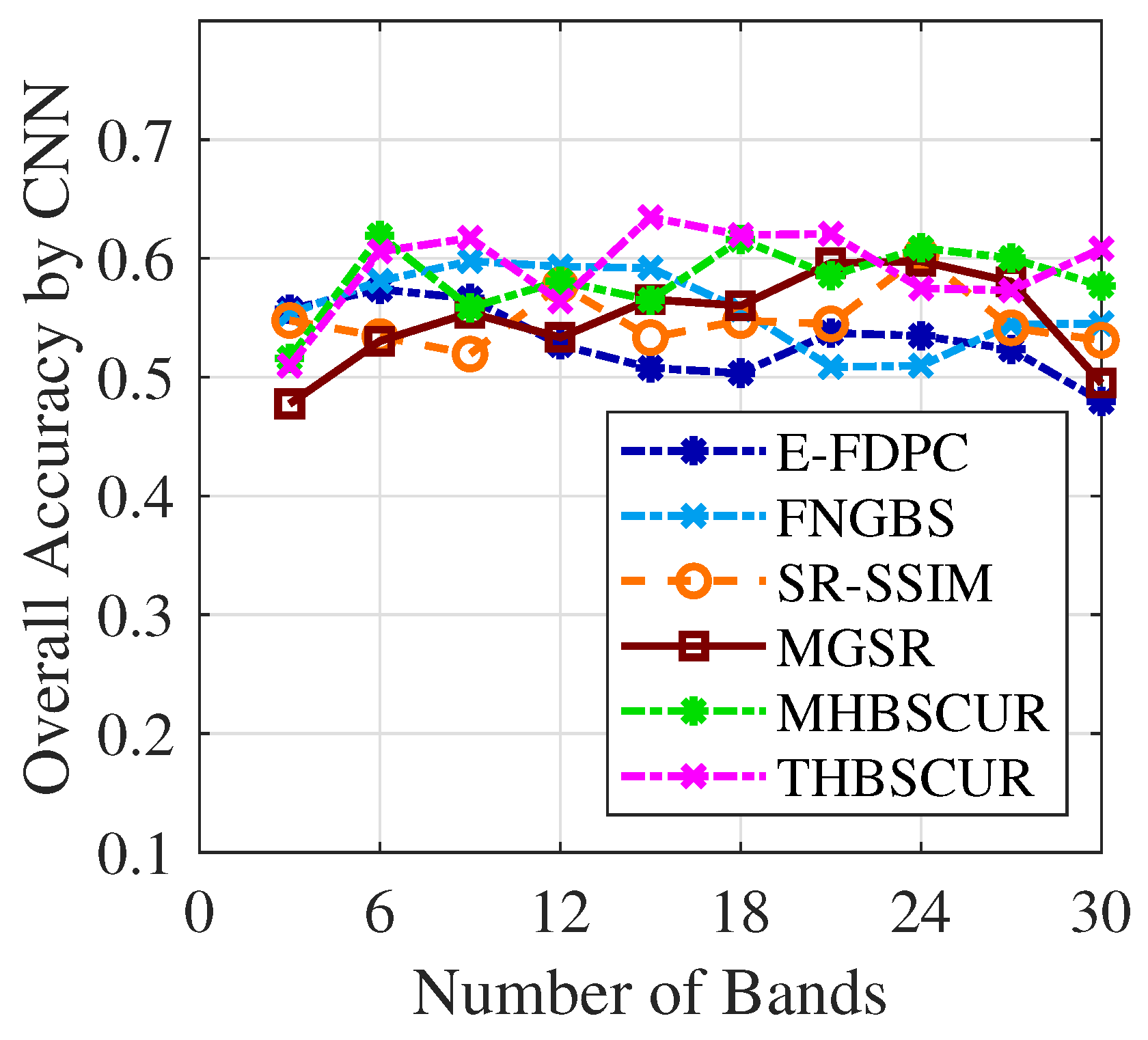
In addition to SVM and KNNs, we also calculated the overall accuracy with CNN as the classifier. In this experiment, we evaluated the performance of the previously considered methods on the Indian Pines dataset. Figure 14 plots the resulting OA curves. For the Indian Pines dataset, it is difficult to distinguish the performance of the different methods, as the accuracy curves are closely clustered. However, the proposed method demonstrated high overall accuracy across different numbers of selected bands as compared to the state-of-the-art methods. Interestingly, CNN classification in this case reported lower overall accuracy than SVM or KNNs classification for the same selected bands.

The CNN network utilized here consists of two convolutional layers with 6 and 16 filters respectively, with each followed by ReLU activation, batch normalization, and max pooling. These layers extract hierarchical spectral features from the input bands. The convolutional layers are followed by three fully connected layers of sizes 120, 84, and k (number of bands), with ReLU activations between them. The final layer uses softmax activation for multiclass classification. The network was trained using the Adam optimizer for 25 epochs, with a learning rate schedule that dropped by a factor of 0.1 every 15 epochs. After training, the network classified the test data, and the overall accuracy was calculated as the proportion of correctly classified samples.

It is worth noting that while CNN demonstrated lower accuracy than SVM and KNNs, it still yielded decent results. This performance could potentially be improved through further optimization of the network architecture and training process.

Other classifiers that have been used to evaluate the performance of hyperspectral band selection in the literature include Classification and Regression Trees (CART) and Linear Discriminant Analysis (LDA) [48,49,50]. CART is a non-parametric decision tree learning technique that produces either classification or regression trees depending on whether the dependent variable is categorical or numeric [51]. It recursively partitions the feature space into subsets where the instances share similar values of the target variable. LDA is a method used to find a linear combination of features that characterizes or separates two or more classes of objects or events [52]. The resulting combination may be used as a linear classifier or for dimensionality reduction before later classification.

Both CART and LDA have been applied to hyperspectral data classification tasks to assess the effectiveness of band selection methods, as they offer different approaches to the classification problem and can provide insights into the discriminative power of the selected spectral bands. Ultimately, we chose to report results from SVM and KNNs due to their robust performance across various datasets and their ability to achieve consistent performance evaluation without extensive hyperparameter tuning or architectural modifications.

6. Conclusions

The high dimensionality and redundancy inherent in hyperspectral imaging data demand effective band selection strategies to ensure computational efficiency and data interpretability. This work introduces a novel tensor-based band selection approach that leverages G3DTV regularization to preserve spatial–spectral smoothness while employing tensor CUR decomposition to enhance processing efficiency and maintain low rankness. Our method stands out by preserving the tensor structure of HSI data, thereby avoiding inefficient conversions between tensors and matrices, and directly addresses spectral redundancy in the tensor form. This approach maintains the multidimensional integrity of the data, making it well suited for a wide range of datasets encountered in practical applications.

In our discussion, we emphasize several key contributions. We highlight the effectiveness of Bayesian Optimization for parameter tuning, which significantly improves the robustness and performance of our method. In addition, we underscore the importance of careful parameter selection, providing insights into how different parameters impact algorithm performance. We also address the challenges posed by noisy HSI data, proposing modifications to enhance resilience in real-world scenarios. Furthermore, we explore alternative methods for the second phase of our algorithm, which offers potential avenues for further performance improvements.

In future work, we aim to develop an accelerated version of our algorithm to further improve its efficiency. We also plan to investigate various importance sampling schemes within the t-CUR decomposition and examine how gradient tensor sparsity affects band selection accuracy.