Article

Mapping Four Decades of Treeline Ecotone Migration: Remote Sensing of Alpine Ecotone Shifts on the Eastern Slopes of the Canadian Rocky Mountains

1
Department of Geography and Environment, University of Lethbridge, Lethbridge, AB T1K 3M4, Canada
2
Department of Physics and Astronomy, University of Lethbridge, Lethbridge, AB T1K 3M4, Canada
3
Canadian Centre for Behavioural Neuroscience (CCBN), University of Lethbridge, Lethbridge, AB T1K 3M4, Canada
4
Agriculture and Agri-Food Canada Research and Development Centre, Lethbridge, AB T1J 4B1, Canada
*
Author to whom correspondence should be addressed.
Remote Sens. 2025, 17(24), 4004; https://doi.org/10.3390/rs17244004
Submission received: 4 September 2025 / Revised: 30 October 2025 / Accepted: 27 November 2025 / Published: 11 December 2025
(This article belongs to the Section Environmental Remote Sensing)

Highlights

What are the main findings?
  • Over the past four decades (1984–2023), the Alpine Treeline Ecotone (ATE) has increased by 13.32% (~199 km2), with substantial increases in the Bow and Athabasca watersheds, as well as significant gains in the northern aspects of the Eastern Slope of the Canadian Rocky Mountains (ESCR).
  • The study developed and implemented the Alpine Treeline Ecotone Index (ATEI) using Landsat imagery and Google Earth Engine (GEE), a novel spatial method that combines NDVI gradients, elevation, and logistic regression to detect and monitor changes to ATE.
What are the implications of the main findings?
  • The responses of ATE migration to climate change vary across aspects and watersheds and are shaped by microclimate, disturbances, and topographic conditions, while the ATEI remains a reliable remote-sensing tool for long-term vegetation monitoring in fragile alpine ecosystems.
  • The upward expansion of ATE zones may affect regional hydrology and watershed dynamics, altering snowmelt timing, runoff patterns, and downstream water availability.
  • For ecological forecasting and biodiversity conservation, understanding spatial shifts in treeline zones is essential, particularly in sensitive alpine habitats.
  • This research can contribute to the development of evidence-based policies, environmental monitoring, and adaptive land management strategies in mountainous regions affected by climate change.

Abstract

Alpine treeline ecotones (ATEs) are critical ecological boundaries that are highly sensitive to climate change, yet their long-term spatial dynamics remain understudied in mountainous regions. This study investigates four decades (1984–2023) of ATE elevational shift along the Eastern Slopes of the Canadian Rocky Mountains (ESCR) using the Alpine Treeline Ecotone Index (ATEI), developed by integrating NDVI gradients, elevation data, and logistic regression. Multi-temporal Landsat composites and Shuttle Radar Topography Mission (SRTM) data were processed in Google Earth Engine (GEE) to map ATE boundaries over nine composite intervals. Results show a 13.32% increase in ATE area (from 1494.17 km2 to 1693.19 km2), indicating a general upslope expansion consistent with a warming climate and extended growing seasons. Although the Mann–Kendall test did not reveal a significant monotonic trend in area change (neither upward nor downward) (p-value > 0.05), notable spatial variability was observed (approximately 8 km2/year). North-facing aspects exhibited the greatest mean elevation gain (+40.21 m), and significant ecotonal changes occurred within the Bow and Athabasca watersheds (p < 0.05), which are equal to around 416 and 452 km2, respectively. These findings highlight the complex, aspect- and watershed-dependent nature of alpine vegetation responses to climate forcing and demonstrate the utility of ATEI for monitoring vegetation biodiversity shifts in high-elevation ecosystems.

1. Introduction

The Alpine Treeline Ecotone (ATE) is a transition zone between subalpine closed-canopy forests and alpine tundra, representing one of the boundaries of highly sensitive climatic responses in mountain ecosystems [1,2]. ATE is influenced by several abiotic and biotic factors, including temperature gradients, soil moisture, solar radiation, snowpack retention, seed dispersal limitations, and the physiology of individual species [3,4,5,6,7]. Because of these conditions, vegetation structure is affected, tree height and density are limited, and seedling recruitment and krummholz formations are characterized in distinct zones [8]. As global temperatures continue to rise, the ATE will move upward at higher elevations, thereby affecting the ecological structure, biodiversity, and hydrological processes of mountains [8,9,10].
The Eastern Slopes of the Canadian Rocky Mountains (ESCR) play a crucial role in regulating ecosystem services, biodiversity, and water resources. This region also continues to provide subregional ecological connectivity and headwaters for important river basins, such as the Bow, Athabasca, Red Deer, and North Saskatchewan River Basins [11]. In Alberta, the ESCR spans over 60,000 km2, and contains barrier features that maintain important microclimates due to steep elevation gradients, slope and aspect variability, as well as disturbances caused by wildfire, insect outbreaks, and deglaciation [12,13,14]. Several of these processes interact with one another and restrict ecotone migration. Therefore, these processes should be analyzed at a regional level, on a scale spatially and temporally relevant to ecotone shifts.
The spatial–temporal approximation of ATE in ESCR is highly influenced by the human context. For many decades, anthropogenic activities have intensified in this area, including recreation development, forest resource extraction, open-pit coal mining, fire suppression policies, and infrastructure development, which has resulted in habitat loss and vegetation disturbance [15,16,17,18,19,20]. Recreational use of land (e.g., hiking, skiing, resort development) has contributed to the alteration and/or degradation of vegetation within hiking areas, soil compaction due to ski runs, and modified microclimates near the treeline [21,22,23]. The practice of logging and road construction has further fragmented montane and subalpine forests, which may have facilitated or suppressed tree migration depending on the site conditions [24]. In addition to recreational use, fire suppression over the last century has reduced natural disturbance regimes that have historically restricted forest advancement and has permitted upward forest encroachment in some areas [25,26]. The changes in the landscape due to human activities are further intertwined with climate factors to modify the direction and/or magnitude of treeline changes and contribute to the spatiotemporal dynamics and patterns of ATEs.
ATE’s biological complexity is further enhanced by several additional factors, including mycorrhizal relationships, genetic variation among populations, and the evolutionary life history strategies of species founding treelines, such as Picea engelmannii and Abies lasiocarpa [27,28,29]. Both species have K-selected life histories, which implies that they invest in very slow growth and infrequent reproduction, which limits their ability to react quickly to changes on a local scale. A disturbance may also serve as both a barrier or a facilitator of ATE migration, so the net impact on ATE migration will depend on the intensity and timing of disturbances [30,31,32]. Thus, the net shift in the ATE dynamic at any place will be derived from a synthesis of climate behavior and fine-scale ecological and disturbance behaviors.
In studies conducted with the ESCR, localized upward shifts of treelines and treeline ecotones have been observed utilizing dendrochronology sampling, localized field surveys, and repeat oblique photography. While such studies provide important insights, they are not spatially comprehensive [13,29,33]. There is a lack of large-scale multi-decadal studies that integrate geospatial techniques with bioclimate and climatic changes to understand these changes better. With the advent of new remote sensing tools, such as Landsat imagery archives and Google Earth Engine (GEE), innovative space–time tools can be used to monitor vegetation change and land cover change in areas of high relief/remote alpine regions [34,35].
An innovative approach model for ATE detection is the Alpine Treeline Ecotone Index (ATEI), which combines two spatial gradients (Normalized Difference Vegetation Index (NDVI) and elevation) with logistic regression to measure the location and magnitude of the ecotone transition zone [36]. Furthermore, the ATEI incorporates the interactions of vegetation structure with terrain in a way that simple threshold methods do not, and it accommodates local spectral response variability. Finally, by using the ATEI over time, it is possible to examine subtle upward shifts and areas that have expanded or reduced, and to assess changes resulting from climatic factors rather than disturbances.
The purpose of this study is to map and capture the last four decades of ATE migration through the ESCR due to climate change and anthropogenic and natural disturbances, using geospatial methods. Further, this study employed a geospatial workflow on GEE to quantify and qualitatively describe the changes in ecotone zones across slopes, aspects, and spatial variability among watersheds using Landsat-based NDVI and Shuttle Radar Topography Mission (SRTM) elevation. In addition, we explored how climate change and disturbance interact and contribute to variations across the landscape. This research aims to accomplish the following objectives:
1—Map ATE boundaries over nine composite time intervals.
2—Explore altitude trends across the eight slope aspects.
3—Determine watershed scale variation to identify areas characterized by significant ecotonal change.
Finally, this research result will provide important information for future mountain ecosystem resilience and help in understanding how ecotone systems respond to climate and environmental drivers.

2. Materials and Methods

2.1. Study Area

This research focuses on the Eastern Slopes of the Canadian Rocky Mountains, a land area of 61,158.60 km2 that includes the headwaters of the Bow, Athabasca, Red Deer, Oldman, and North Saskatchewan watersheds. The study area extends between 48°59′34.27″N and 53°56′35.16″N at latitude and 119°06′2.5″W and 113°29′54.47″W at longitude, and the study area ranges in elevation from 985 to 3710 m (Figure 1).
In order to determine the eastern boundary of the ESCR, provincial hydrological maps, watershed boundaries, and stream gauge station elevations that ranged between 900 and 1200 m were used. The region includes dominating slope aspects on the north, northeast and east-facing slopes, which contribute to microclimatic gradients and snow retention regimes. Ecologically, the ESCR covers both the Rocky Mountain and Foothills Natural Regions and includes mixed coniferous forests characterized mainly by Picea engelmannii (Engelmann spruce), Abies lasiocarpa (subalpine fir), Pinus contorta (lodgepole pine), and Populus tremuloides (trembling aspen), in addition to krummholz at the ATEs elevations (upper elevations) [37,38].
There is a complex alpine–subalpine climate in the study area, with cold, snowy winters and short, mild summers [39]. Climate in an alpine environment is strongly influenced by orographic precipitation patterns, with higher precipitation amounts found at the windward elevations and drier conditions in the leeward valleys, and lower elevation sites, such as Calgary, Lethbridge, and Alberta [40]. At higher elevations, temperatures can be as low as −5 °C, while at lower foothill locations, temperatures can be as high as 22 °C, and total annual precipitation can range from 280 mm to over 4300 mm [41], with substantial amounts of snow falling at higher elevations [42]. In the Canadian Rockies, high-elevation subalpine and alpine sites experience very short frost-free periods, typically less than 70–90 days, which strongly limits the establishment and growth of plant communities near and above the treeline [29,43]. Over the past four decades, regional climate studies have documented significant warming in the Canadian Rockies, resulting in an increase in mean temperatures and an earlier melting of snow [42].

2.2. Data Sources

In this study, satellite optical imagery, topographic data, and fine-resolution reference imagery were used to monitor and measure changes in the ATE throughout the ESCR between 1984 and 2023. All geospatial datasets were accessed and processed in GEE, a platform for cloud computing and processing for geospatial analysis, along with access to multi-decadal potential satellite observations of the Earth [44].

2.2.1. Landsat Satellite Imagery

The Landsat Surface Reflectance Tier 2 Collection was the primary source of remote sensing data, specifically from Landsat 5 Thematic Mapper (TM) and Landsat 8 Operational Land Imager (OLI). These sensors provide consistent surface reflectance values at 30 m spatial resolution, making them well-suited for long-term landscape-scale vegetation monitoring [45,46]. To ensure radiometric consistency among sensors and over time, both series of images were calibrated, and only atmospherically corrected Level 2 imagery was utilized [47,48].
It was determined that the months of July–September reflected conditions of maximum phenological activity in our area and the least seasonal variation from a time series analysis. This study used the Best Available Pixel Compositing method [49] to create nine temporal composites (1984–1989 (Composite 1), 1990–1995 (Composite 2), 1996–1998 (Composite 3), 1999–2002 (Composite 4), 2003–2006 (Composite 5), 2007–2011 (Composite 6), 2013–2015 (Composite 7), 2016–2020 (Composite 8), and 2021–2023 (Composite 9)). These composites are based on the median reflectance for the interval and are intended to remove the effects of cloud cover, noise, and acquisition voids.

2.2.2. Shuttle Radar Topography Mission (SRTM)

Topographic information was derived from the Shuttle Radar Topography Mission (SRTM) at a resolution of 30 m. A digital elevation model (DEM) created by STRM is then used to calculate elevation, slope, and aspect variables. There is a strong correlation between terrain dimensions and vegetation, particularly in mountainous environments [50,51,52]. Rodríguez et al. (2006) [53] demonstrate that SRTM datasets are suitable for modeling high-resolution ecological processes in mountainous ecosystems of North America.

2.2.3. High-Resolution Reference Imagery

High-resolution Google Earth images (approximately 0.5 m spatial resolution, 2021–2023) were used to confirm the accuracy of the ATEI-classified zones. An analysis of a stratified random sample of 386 Landsat pixels was conducted based on canopy density, the presence of krummholz forms, and the elevation limitations. Based on the complexity of this landform and the logistical impracticality of in situ field validation, this reference dataset was used as a surrogate for in situ field validation. Furthermore, previous studies have used similar validation methods in alpine treeline studies [29,33].

2.3. Methods

This study used a multistep remote sensing and geospatial analysis process to identify and quantify changes in ATE in the ESCR between 1984 and 2023. As part of the methodology, we applied spectral indices, topography modeling, and statistical analysis using GEE [36], ArcGIS Pro 3.6, and Python scripting (V3.9). The complete workflow is illustrated in Figure 2.

2.3.1. Max NDVI

From each Landsat composite, the maximum NDVI was calculated for the summer months (June, July and August) using the red and near-infrared bands. In addition to being a well-documented proxy for canopy greenness, vegetation density, as well as photosynthetic activity, NDVI is particularly effective in detecting slight vegetational shifts within ecotonal zones [35,54].
NDVI values were derived using the following standard equation:
N D V I = N I R R e d N I R + R e d
The maximum NDVI value for each pixel during the growing season was retained, capturing peak canopy development and minimizing snow-related bias. NDVI served as the basis for two components (C1 and C2) of the ATEI used to delineate ecotonal areas [36].

2.3.2. Vegetation Indices and Ecotone Delineation

A standard formulation [55] was used to calculate NDVI for each composite. This is because NDVI not only is a good indicator of photosynthetic activity, but also is a good indicator for canopy density, which allows us to distinguish between closed-canopy subalpine forests, sparsely vegetated ecotones, and alpine tundra.
In the next step, we calculated the magnitude and direction of the gradient of the NDVI. To improve delineation, NDVI values were combined with elevation model (DEM). In order to exclude areas below 1680 m (low elevation ATE), a masking step was undertaken. In applying this masking step, the study was able to restrict its analysis to only treeline transition zones that are ecologically feasible. As part of the DEM analysis, aspect layers were extracted and ecotone pixels were stratified into eight aspect classes (N, NE, E, SE, S, SW, W, NW), the magnitude and direction of elevation change were calculated, and the sudden changes in NDVI were calculated (Theta (θ)).

2.3.3. Alpine Treeline Ecotone Index (ATEI)

The ATEI quantitatively assesses the geographical location of treeline ecotones as identified within remote sensing data, by incorporating three components (C1, C2, and C3), all of which aim to measure the characteristics found within the ecotone. Firstly, C1 is designed to assess abrupt spatial gradient change of NDVI across the ecotone, as there is an abrupt change in vegetation cover when transitioning from montane forest to alpine tundra. To do this, NDVI gradient magnitude (C1) measures abrupt spatial changes in NDVI along elevation gradients based on this equation:
C 1 = Δ f N D V I Δ d = N D V I t u n d r a N D V I f o r e s t d t u n d r a d f o r e s t
where d is the ground distance (m) between the two sampled points across the ecotone.
C2 contributes intermediate NDVI values associated with the transitional space of the vegetated region within the ecotone. We modeled the intermediate NDVI values using a Gaussian function that is centered on the NDVI values associated with vegetation found within ATE. Thus, Gaussian NDVI distribution modeled the likelihood of ecotone presence as a function of NDVI, fitted using Gaussian probability:
To generate component C2, the Gaussian function was applied to the smoothed NDVI values following this equation:
C 2 = φ e f N D V I b 2 2 c 2
In this case, φ represents the height of the peak of the Gaussian curve, e represents the base of the natural logarithm, NDVI represents the smoothed NDVI value, and b and c represent the predefined parameters (φ =1, c = standard deviation of NDVI values, and b = median of NDVI values).
To calibrate the C2 component for our study area, we initially selected 386 Landsat 8 pixels randomly. To ensure a representative sample size for calibration results, the study considered statistical principles (finite population correction (FPC)) to determine how many pixels should be selected from the study area [56]. The pixels were also distributed uniformly and homogeneously throughout the area. A human visual interpretation of high-resolution imagery from 2021 to 2023 was used two times (to minimize human bias) to determine the location accuracy of each calibration pixel. Finally, the mean value of those results was utilized in the calibration formula.
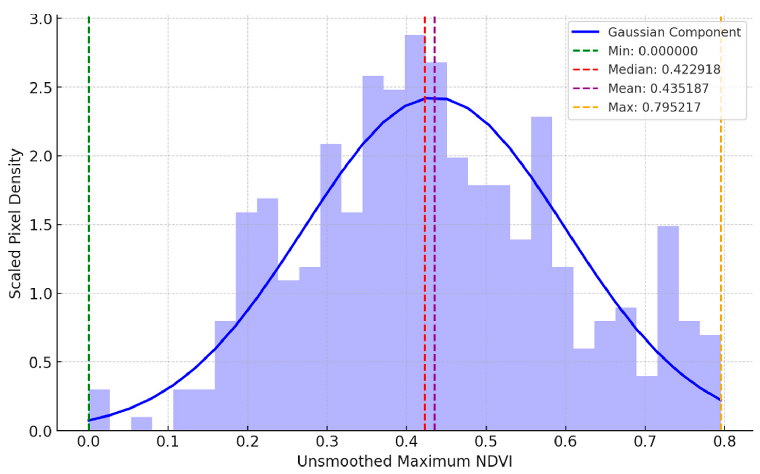
To refine the Gaussian function of the second ATEI component (C2) based on the distribution of unsmoothed maximum NDVI values, only pixels classified within the ATE zone were considered (Figure 3). According to Figure 3, the median NDVI value of pixels within the ATE was approximately 0.42, represented by the red dashed line, while the standard deviation of the component was calculated to be 0.16. Accordingly, for the Gaussian function of this component, we set b = 0.42 and c = 0.16. Therefore, C2 would be close to its maximum value (1) if the pixel was located within the ATE.
Lastly, C3, also known as the spatial covariation of NDVI and elevation, quantifies the orientation difference between NDVI and elevation gradients, as NDVI typically decreases with elevation along ATE zones. This component was calculated by considering the angle (θ) between the local image gradients of NDVI and elevation. The difference in gradient directions between the NDVI gradient direction and the elevation gradient direction was computed. The difference between the NDVI gradient direction and the elevation gradient direction was computed and is presented using the following equation:
C 3 = ( 1 cos θ ) n 2 n
where C3 is the spatial covariation of NDVI and elevation, and θ is the angle between NDVI gradient direction and elevation. ‘n’ is potential ATEs and disturbed areas, which is a constant value (10). Based on sensitivity analyses and calibration, we set the exponent to n = 10, which provides steep angular selectivity when C3 ≈ 0.5 at θ ≈ 150° and >0.9 by θ ≥ 170°, thereby emphasizing near-anti-parallel NDVI–elevation gradients characteristic of ATEs while suppressing oblique, noise-driven alignments.
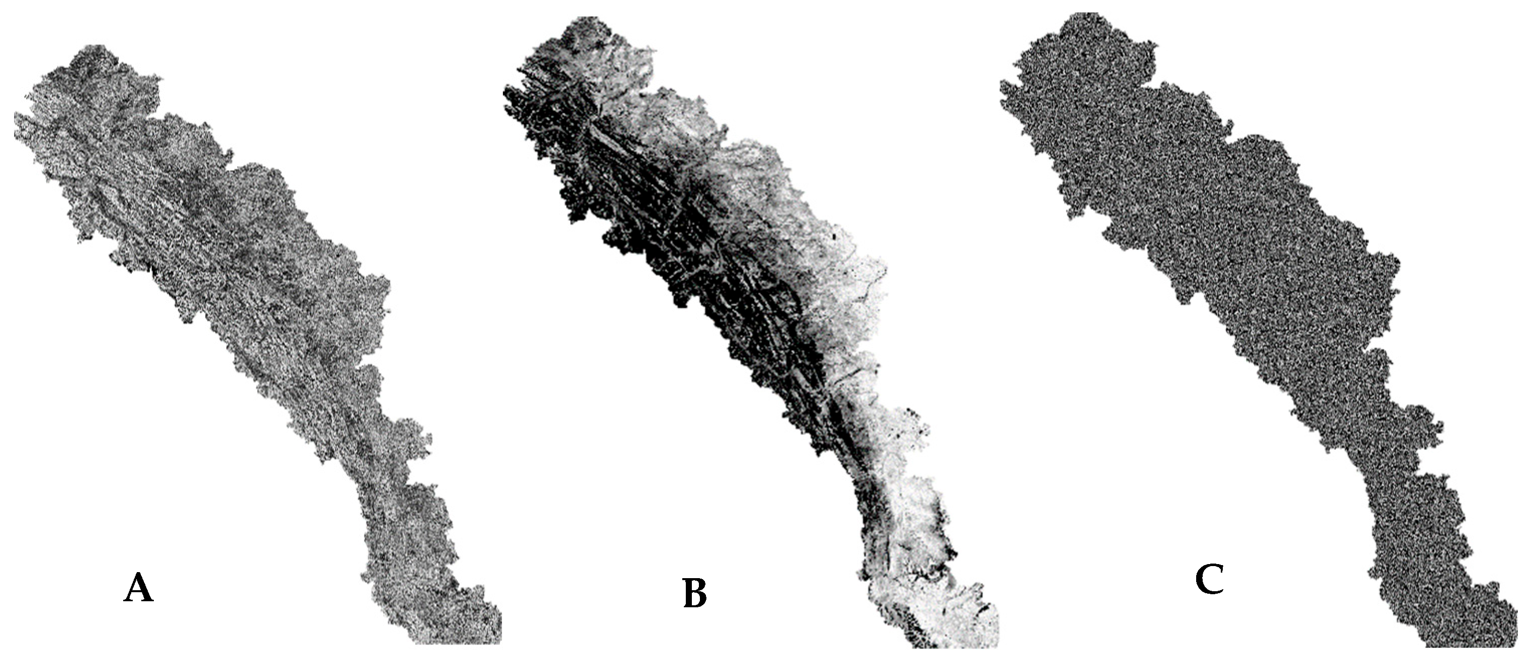
Due to the large difference between the gradient component (C1) and components C2 and C3, we decided to standardize each component as follows (Figure 4):
S = x μ σ
At each Landsat pixel, x represents an ATEI component values (C1, C2 or C3), μrepresents the spatial average of that component across all pixels (the mean value of all pixels), and σ represents the spatial standard deviation.
This study implemented the A T E I using a binomial logistic regression model, which integrates the standardized components to predict the probability that a pixel will be located within the ATEs. After standardizing three components, the A T E I was calculated for each period of time series analysis using a binomial logistic regression to predict the A T E I zone (Figure 5):
A T E I = ( e x ) ( e x + 1 )
x = b 0 + b 1 × C 1 + b 2 × C 2 + b 3 × C 3
where ATEI is a logistic function used to transform a linear combination of variables into a value between 0 and 1, e x is the exponential function, x is a linear combination of the components (C1, C2 and C3), and b0, b1, b2, and b3 are intercept and fixed parameters (estimated from data), respectively. It should be noted however that these values were empirically derived based on the training of field data within the study domain and are fixed parameters of the equation.

2.3.4. Watershed-Level Aggregation

ATEI outputs were summarized by major watershed boundaries (Bow, Athabasca, Red Deer, Oldman, North Saskatchewan) to assess spatial variability across ecological subregions. The total ecotone area and the change in average elevation were calculated for each watershed. We used a Chi-square test to determine whether there was a statistically significant difference in the change patterns between all watersheds. The Chi-square test was employed to assess the geographic heterogeneity of ATE changes among different watershed units. The data included counts of ecotonal changes (for example, the presence or absence of significant ATE expansions) between discrete spatial categories (Bow, Athabasca, and other basins). In assessing whether the observed distribution of changes differed significantly from an expected random distribution, the Chi-square test provided a suitable non-parametric test, as it allowed for categorical differences between independent groups and highlighted areas of the watershed which experienced disproportionate changes in the environment. Thus, this test facilitates the evaluation of spatially non-random patterns of treeline dynamics that may be explained by localized climatic, topographic, or anthropogenic processes and impactors.

2.3.5. Validation and Accuracy Assessment

A stratified random sample of 386 pixels was used three times to assess classification accuracy. Each time, the data was validated by an expert knowledge method against high-resolution Google Earth imagery (0.5 m) from 2021 to 2023. The visual interpretation of ATE was conducted to calculate the final accuracy of maps. In fact, ATE differs from dense forests and tundra due to its canopy structure, density, texture and elevation changes. Finally, a classification accuracy of 81.30% was calculated based on three validation attempts (81.86%, 79.07%, and 82.98%, respectively).

3. Results

3.1. Alpine Treeline Ecotone Mapping over Nine Composite Intervals

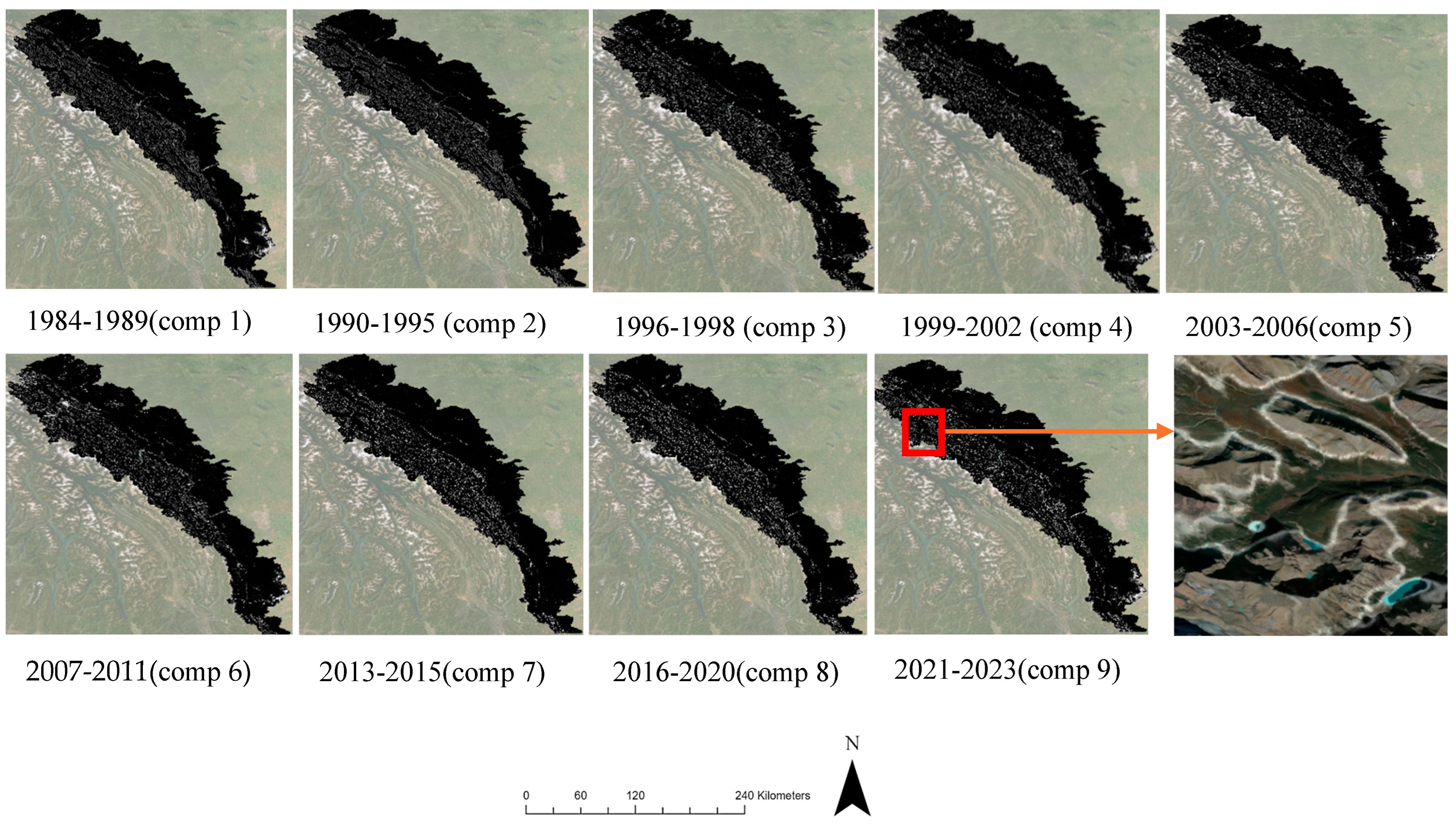
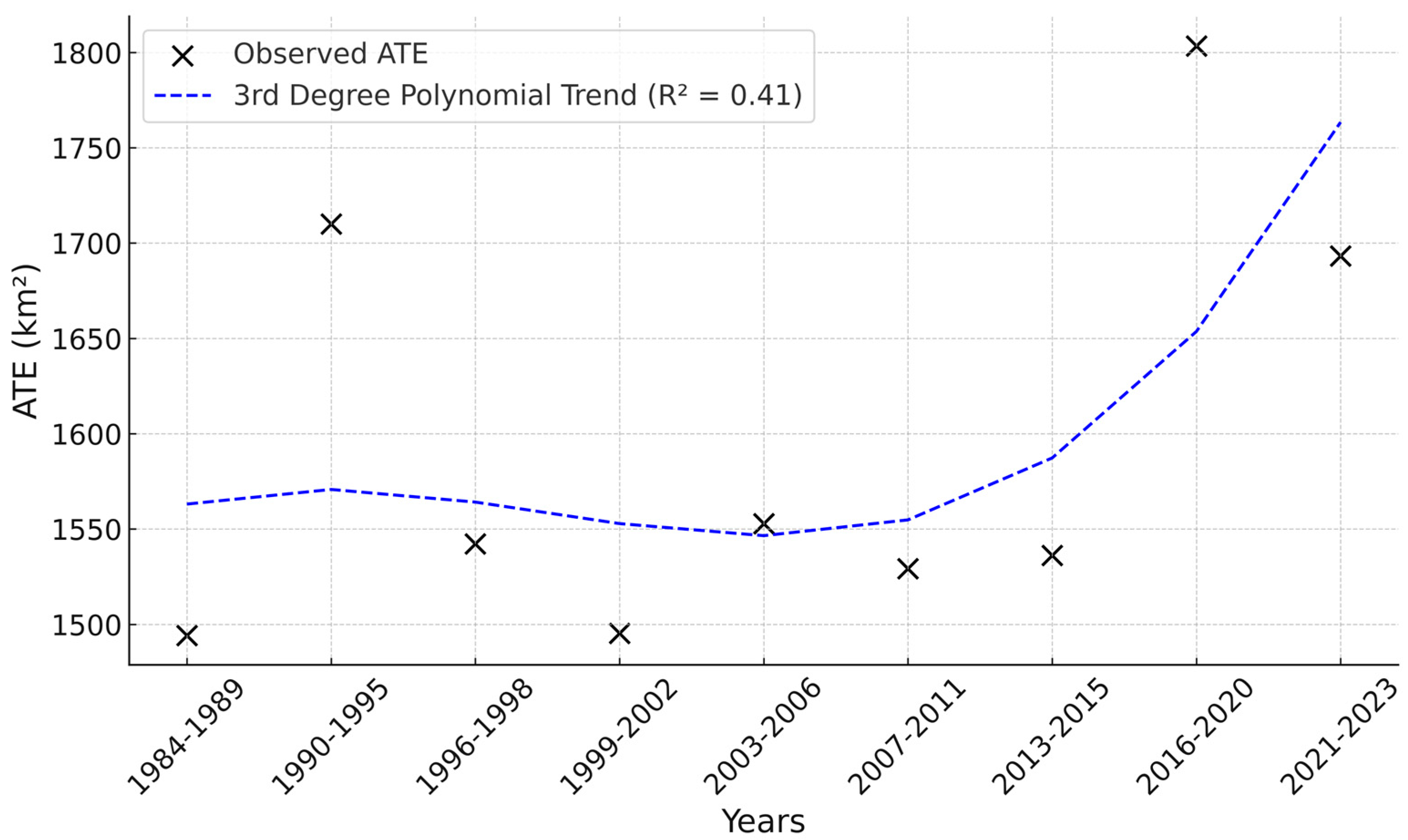
As a result of utilizing the ATEI in nine composite periods (1984–2023), significant spatial-temporal variability in ecotone distribution was observed along ESCR (Figure 5 and Figure 6). During the first time period (1984–1989), the area of ATE was around1494.0 km2; most patches of ATE were located along mid-to upper-surface positions in Jasper and Banff National Parks, while patches of ATE were found in Kananaskis Country, as well as in and around Crowsnest Pass. During the last period (2021–2023), the total mapped ATE area was approximately 1693 km2, which represented a net gain of approximately 195 km2 (+13.32%) over four decades. We also conducted a Mann–Kendall statistical analysis on our dataset to compare the results. The statistical model demonstrated that there has not been a statistically significant monotonic trend in the data (neither upward nor downward) (p-value > 0.05). Based on this test, there is no strong evidence of a monotonic trend (either increasing or decreasing) over time in the ATE distribution data.

3.2. Variation in Altitude Across Different Aspects

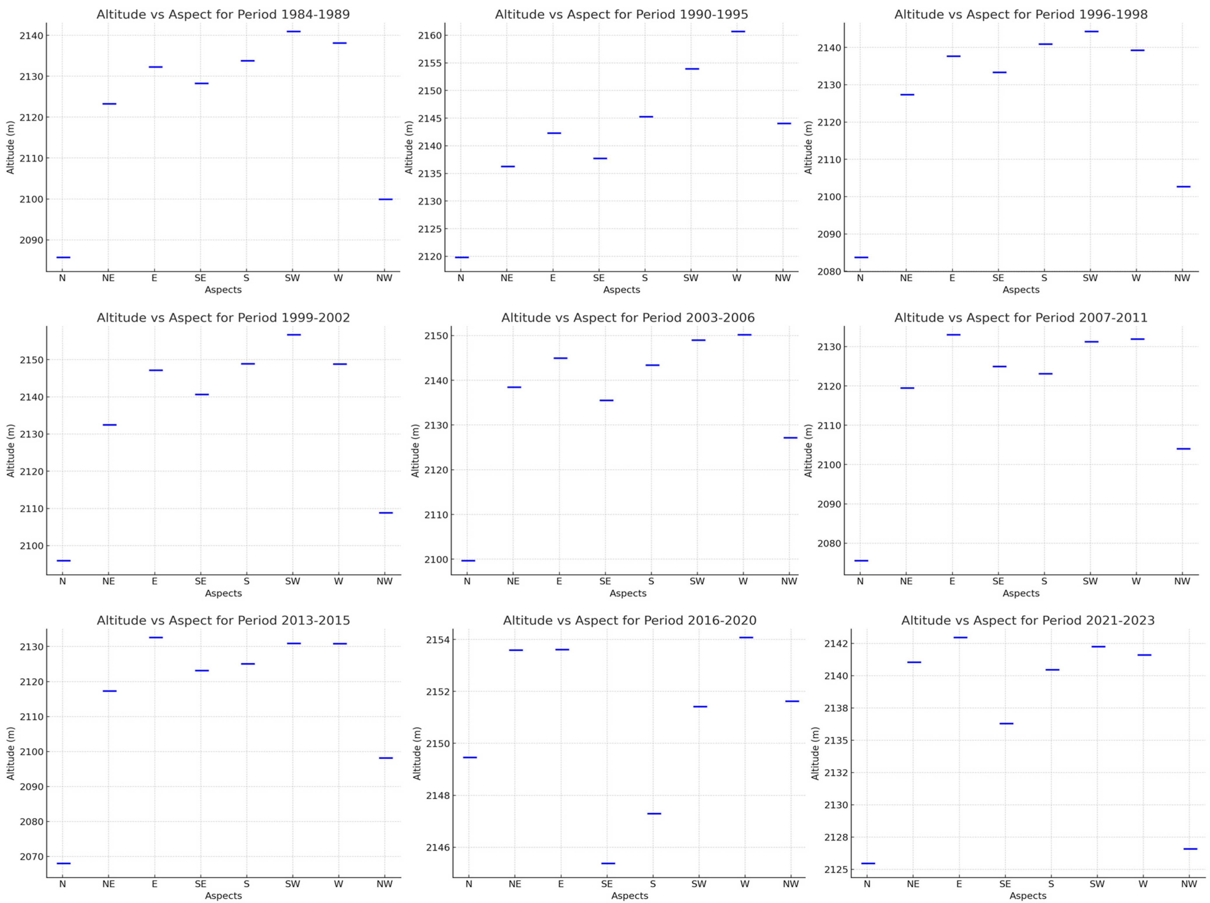
Analyzing the ATE elevation on eight slope aspects (N, NE, E, SE, S, SW, W, NW) indicated a consistent, but varied, elevation change pattern throughout 1984–2023 (Figure 7, Table 1). The mean elevation of ATE across all aspects stayed within a narrow range of 2067–2160 m. The mean elevation of ATE decreased from northerly aspect (N, NE, NW) to southerly aspect (S, SE, SW) due to less solar radiation exposure, cooler microclimate conditions, and greater available moisture on north-facing slopes compared to south facing slopes. As a result of greater exposure to solar radiation, warmer surface conditions, and a longer growing season with sufficient moisture, the ATE was consistently higher on south-facing slopes.
According to the Mann–Kendall trend analysis, the maximum change in mean elevation occurred on north-facing slopes (+40.21 m), followed by northwest (+27.12 m) and northeast aspects (+18.21 m). Although there is not a monotonic trend that is statistically significant at p < 0.05, the apparent upward shifts across all aspects imply a generalized elevational migration of the ecotone and could reflect regional climate change, where warming temperatures are promoting upslope tree establishment, but it is not the only factor for this migration [29,33,57,58].
Additionally, results indicate that the magnitude of change differed across aspects (typically, the northern slopes exhibited the greatest gains even when starting with a lower mean elevation). According to the results, trees are growing where previously colder, more restrictive environments had existed. The change over time in elevation among aspects may reflect both climate variables (temperature, precipitation, solar radiation) and natural disturbances (wildfires, insect outbreaks, landslides). Stable periods with almost no change between aspects could indicate more stable conditions in the environment, while periods where aspect differences were most pronounced also indicated the greatest climatic or disturbance-driven change. It is evident from the results that the ATE has expanded upward in all aspects, and over the past 40 years, we have observed an increase in the greening of the eastern slopes of the Canadian Rockies [12,29,33].

3.3. Watershed-Scale Variation in Ecotonal Change

We calculated the 40-year change in each pixel based on the ATE raster data from 1984 to 2023 (Table 2). The purpose of this study was to illustrate the spatial distribution of the ATE and the characteristics of the spatial changes over time in ESCR. We also analyzed the change using ArcGIS Pro 3.6 software, followed by a change trend analysis of ATE (Figure 8).
Based on the analysis of the spatial variation of ATE across five watersheds in the ESCR between 1984 and 2023, it was found that ATE change trends were significantly influenced by spatial heterogeneity. Based on the results of the statistical analysis (Chi-square test in Python 3.9) at a 95% confidence level, two watersheds, Bow and Athabasca, exhibited highly significant p-values of 0.0008 and 0.0025, respectively. According to these results, the observed increases and decreases in ATE are unlikely to have been due to chance, and systematic drivers, such as climate change or anthropogenic stressors, may have influenced these trends.
Conversely, the Old Man, Red Deer, and North Saskatchewan watersheds showed non-significant p-values (0.100, 0.631, and 0.248, respectively), suggesting that fluctuations in these regions could largely be attributed to random fluctuations rather than consistent changes in direction. Moreover, there was a total change (increases and decreases) of 415.75 km2 in the Bow watershed while 451.94 km2 was observed in the Athabasca watershed, highlighting the dynamic ecotonal transitions in these two watersheds. Red Deer watershed, on the other hand, had the smallest change in total area of 120.25 km2, with its p-value strongly supporting random variation. Thus, these findings suggest that targeted ecological studies should be conducted in the Bow and Athabasca watersheds to gain a better understanding of the mechanisms underlying ATE dynamics (Table 2).

4. Discussion

The study presents a novel, multi-decadal assessment of ATE migration on the ESCR between 1984 and 2023. Through the integration of NDVI gradients, elevation data, and slope aspects, we observed three key patterns of change: a measurable expansion of ATE areas, distinct altitudinal trends across slope aspects, and significant variability in ATE dynamics across watersheds.

4.1. Utility of the ATEI in Monitoring Climate-Driven Transitions in Mountain Ecosystems

The ATEI has become a valuable indicator of transitional forest-tundra zones in mountain ecosystems, such as the ESCR. The ATEI provides researchers with a standardized, spatially explicit method for mapping and monitoring treeline ecotones across expansive and diverse landscapes, such as those accessible through remote sensing platforms, including LiDAR and multispectral satellite imagery [14,36]. The ATEI can be especially advantageous in understanding responses to climate change due to its ability to detect vertically scale-dependent vegetation structure (e.g., upward resulting shifts in treeline, biomass accumulation, infilling in previously tundra-dominated areas) [8,13]. Moreover, the ATEI provides a means to understand changes in ecosystem transitions temporally, allowing long-term ecological monitoring and separating climatic impacts from other disturbance-based changes (fire, avalanche, insect outbreaks) [29]. Also, the index can be used to enhance the predictive capacity of the dynamics of ecotones in future climate change scenarios using machine learning approaches (e.g., random forest algorithms). Thus, these features represent several reasons why the ATEI is a useful tool for mountain ecosystems, management options, and climate adaptation efforts in high-elevation regions.

4.2. ATE Expansion and Stability over Time

As a result of climate change scenarios, the overall rise of 199.02 km2 in ATE area over four decades (13.32%) is consistent with recent upward trends in mountain ecosystems occurring worldwide [1,9]. According to this small, but slow, upward trend, especially in upper and mid-elevation areas, extending growing seasons and increasing average temperatures in the ESCR region over a period of four decades have allowed woody and non woody vegetations to establish to the south and eventually move consistently up slope in the ESCR region [29,33,57,58]. It is important to note, however, that the Mann–Kendall test did not detect a statistically significant monotonic trend (p < 0.05), indicating that ATE expansion may occur in a nonhomogeneous manner influenced by episodic drivers (wildfire, insect outbreaks, short-term climate fluctuations, etc.) and/or episodic climate oscillations [59]. Moreover, this increase in ATE may be attributed to global warming and the lengthening of the growing season in this region [8,33,60]. However, a decline in ATE in the ESCR areas can be explained by increasing wildfires and other disturbances, especially in the recent decade. The change detection maps also indicated that the largest upward boundaries occurred in sheltered valleys and leeward slopes in the middle of the study area (Bow and Athabasca) where snow accumulation and snowmelt delay may have prolonged the growing season. There was a relatively continuous movement of vegetation upslope into tundra vegetation in these areas. Furthermore, high-elevation plateaus and ridges exposed to wind had a reduced extent, with a few remaining the same size, due to the influence of microclimates and shallow soils.

4.3. Elevational Differences Among Slope Aspects

We found that slope aspect is a key mechanism in determining ATE elevation, most likely due to differences in solar radiation, microclimate, and soil moisture regimes. A typical pattern was observed for all sampled sites, with the northern slopes (N, NE, NW) having the lowest ATEs (accounting for steeper slopes) and the southern slopes (S, SE, SW) having the highest ATEs positions. Although no statistically significant trends by slope aspect were observed (p > 0.05), the largest absolute elevation increases were observed on slopes with a north-facing aspect (+40.21 m), followed by slopes with a northwest aspect (+27.12 m) and slopes with a northeast aspect (+18.21 m). This could indicate that areas that were previously colder are now more conducive to tree invasion and colonization [33,61]. This confirms previous literature [6] that suggests northern aspects may be more sensitive to warming simply as a result of their previous thermal limits.

4.4. Spatial Heterogeneity in Watershed-Level Ecotonal Change

The change in ecotones at the watershed scale was not spatially homogeneous. Bow and Athabasca watersheds experienced the most dramatic changes, as demonstrated by net changes in area representing 415.75 km2 and 451.94 km2, respectively, with statistical significance (p = 0.0008 and 0.0025). It is possible that this indicates a synergistic effect between factors related to climate change and factors related to elevation gradients and disturbance patterns unique to each watershed (e.g., frequency of wildfires or changes in hydrology). Other watersheds, such as Red Deer and Oldman, exhibited minor or statistically insignificant changes, suggesting more stable ecotonal configurations and/or greater resilience to change during the study period [35]. An analysis of the magnitude and direction of future changes at the watershed scale is crucial to understanding future conservation priorities and resilience planning.

4.5. Drivers and Implications of ATE Migration

According to regional trends in increasing annual temperature and growing season length, the gradual increase in ATE over time appears to be largely due to climatic warming. The changes were heterogeneous across slopes and watersheds, and we did not observe strong monotonic trends. There may be other factors that affect ATE dynamics, such as variation in snowpack, microclimate associated with wind exposure, soil depth, and legacy effects from disturbances, which interact with one another. Similar to other studies, we found ATE migration to be often a non-linear process that depended on broader and local processes [7,27].
From a practical standpoint, the upward movement of the ATE has important implications for biodiversity, carbon storage, and hydrological processes. By replacing alpine tundra with forest species, niche habitats may be minimized and ecological community structures altered, while changes in snowpack accumulation and runoff duration can have significant downstream impacts on the water supply to important river basins in Alberta.

5. Conclusions

This study provides an assessment of the dynamics of the ATE along the ESCR over a multi-decade period. Also, this study demonstrates the utility of the ATE as a spatially explicit and ecologically meaningful tool. The ATE expansion has increased by 13.32% over the past four decades, with the largest changes observed in the Bow and Athabasca watersheds. Ecotone shifts are believed to be a result of a combination of climate warming and possible local enhancement associated with topography and/or disturbance. Although the Mann–Kendall test did not detect statistically significant monotonic trends in either elevation or area change, the observed spatial variability and elevation-dependent aspect patterns demonstrate that ecotones respond to co-occurring biophysical processes and anthropogenic pressures in multiple ways. As a result of integrating NDVI gradients, elevation, and orientation, the ATEI was able to identify subtle changes in vegetation that would otherwise be overlooked when using more traditional binary classification or threshold-based approaches. We concluded that ecotone migration does not follow a linear pattern, nor is it uniform in nature, but is nuanced by slope aspects, disturbance dynamics, and watershed-scale heterogeneity. A long-term, repeated assessment with finer spatial resolutions is required to ultimately drive conservation and adaptive management in fragile alpine regions undergoing change and perturbation as climate variability increases.
Future studies should incorporate disturbance history, such as fires and insect outbreaks, or the interaction of climate and local factors (snow cover, wind erosion, soil, and disturbance legacy) into the model in order to identify the relative contributions of different drivers. In addition, the use of high-resolution UAV or LiDAR data could also assist in the detection of structural vegetation changes not adequately captured by medium-resolution satellite images. Finally, ecological modeling efforts should focus on simulating the dynamics of the ATE under a variety of climatic scenarios to predict how the Canadian Rockies’ landscape will look in the near future.

Author Contributions

Writing—original draft, B.H.; Writing, review & editing, D.L.J., L.S., H.S.R. and A.C. The authors have reviewed and edited the output and take full responsibility for the content of this publication. All authors have read and agreed to the published version of the manuscript.

Funding

This research was funded by 2023–2024 Alberta Innovates Graduate Student Scholarship.

Data Availability Statement

The original contributions presented in the study are included in the article, further inquiries can be directed to the corresponding author.

Conflicts of Interest

The authors declare no conflicts of interest, and the funders had no role in the design of the study; in the collection, analyses, or interpretation of data; in the writing of the manuscript; or in the decision to publish the results.

References

  1. Körner, C. Alpine Treelines; Springer: Basel, Switzerland, 2012; ISBN 978-3-0348-0395-3. [Google Scholar]
  2. Holtmeier, F.; Broll, G. Sensitivity and Response of Northern Hemisphere Altitudinal and Polar Treelines to Environmental Change at Landscape and Local Scales. Glob. Ecol. Biogeogr. 2005, 14, 395–410. [Google Scholar] [CrossRef]
  3. Lechler, L.; Rixen, C.; Bebi, P.; Bavay, M.; Marty, M.; Barbeito, I.; Dawes, M.A.; Hagedorn, F.; Krumm, F.; Möhl, P.; et al. Five Decades of Ecological and Meteorological Data Enhance the Mechanistic Understanding of Global Change Impacts on the Treeline Ecotone in the European Alps. Agric. For. Meteorol. 2024, 355, 110126. [Google Scholar] [CrossRef]
  4. Huang, M.; Wang, G.; Bie, X.; Jiang, Y.; Huang, X.; Li, J.-J.; Shi, S.; Zhang, T.; Peng, P.-H. Seasonal Snow Cover Patterns Explain Alpine Treeline Elevation Better than Temperature at Regional Scale. For. Ecosyst. 2023, 10, 100106. [Google Scholar] [CrossRef]
  5. Bailey, S.N.; Elliott, G.P.; Schliep, E.M. Seasonal Temperature–Moisture Interactions Limit Seedling Establishment at Upper Treeline in the Southern Rockies. Ecosphere 2021, 12, e03568. [Google Scholar] [CrossRef]
  6. Liang, E.; Wang, Y.; Piao, S.; Lu, X.; Camarero, J.J.; Zhu, H.; Zhu, L.; Ellison, A.M.; Ciais, P.; Peñuelas, J. Species Interactions Slow Warming-Induced Upward Shifts of Treelines on the Tibetan Plateau. Proc. Natl. Acad. Sci. USA 2016, 113, 4380–4385. [Google Scholar] [CrossRef]
  7. Germino, M.J.; Smith, W.K.; Resor, A.C. Conifer Seedling Distribution and Survival in an Alpine-Treeline Ecotone. Plant Ecol. 2002, 162, 157–168. [Google Scholar] [CrossRef]
  8. Griesbauer, H.; Bevington, A. Recent Changes in Forest Structure and Growth at the Alpine-treeline Ecotone in the Rocky and Columbia Mountains of Central British Columbia, Canada. J. Biogeogr. 2024, 51, 677–693. [Google Scholar] [CrossRef]
  9. Harsch, M.A.; Hulme, P.E.; McGlone, M.S.; Duncan, R.P. Are Treelines Advancing? A Global Meta-analysis of Treeline Response to Climate Warming. Ecol. Lett. 2009, 12, 1040–1049. [Google Scholar] [CrossRef] [PubMed]
  10. Andrews, C.; Foster, J.R.; Weiskittel, A.; D’Amato, A.W.; Simons-Legaard, E. Integrating Historical Observations Alters Projections of Eastern North American Spruce–Fir Habitat under Climate Change. Ecosphere 2022, 13, e4016. [Google Scholar] [CrossRef]
  11. Serbu, J.A.; St Louis, V.L.; Emmerton, C.A.; Tank, S.E.; Criscitiello, A.S.; Silins, U.; Bhatia, M.P.; Cavaco, M.A.; Christenson, C.; Cooke, C.A.; et al. A Comprehensive Biogeochemical Assessment of Climate-Threatened Glacial River Headwaters on the Eastern Slopes of the Canadian Rocky Mountains. J. Geophys. Res. Biogeosci. 2024, 129, e2023JG007745. [Google Scholar] [CrossRef]
  12. Davis, E.L.; Gedalof, Z. Limited Prospects for Future Alpine Treeline Advance in the Canadian Rocky Mountains. Glob. Chang. Biol. 2018, 24, 4489–4504. [Google Scholar] [CrossRef]
  13. Roush, W. A Substantial Upward Shift of the Alpine Treeline Ecotone in the Southern Canadian Rocky Mountains. Master’s Thesis, University of Victoria, Victoria, BC, Canada, 2009. [Google Scholar]
  14. McCaffrey, D.R.; Hopkinson, C. Modeling Watershed-Scale Historic Change in the Alpine Treeline Ecotone Using Random Forest. Can. J. Remote Sens. 2020, 46, 715–732. [Google Scholar] [CrossRef]
  15. Cooke, C.A.; Emmerton, C.A.; Drevnick, P.E. Legacy Coal Mining Impacts Downstream Ecosystems for Decades in the Canadian Rockies. Environ. Pollut. 2024, 344, 123328. [Google Scholar] [CrossRef]
  16. Bebi, P.; Kulakowski, D.; Veblen, T.T. Interactions between Fire and Spruce Beetles in a Subalpine Rocky Mountain Forest Landscape. Ecology 2003, 84, 362–371. [Google Scholar] [CrossRef]
  17. Schuster, R.; Germain, R.R.; Bennett, J.R.; Reo, N.J.; Arcese, P. Vertebrate Biodiversity on Indigenous-Managed Lands in Australia, Brazil, and Canada Equals That in Protected Areas. Environ. Sci. Policy 2019, 101, 1–6. [Google Scholar] [CrossRef]
  18. Powers, R.P.; Coops, N.C.; Nelson, T.; Wulder, M.A.; Ronnie Drever, C. Integrating Accessibility and Intactness into Large-Area Conservation Planning in the Canadian Boreal Forest. Biol. Conserv. 2013, 167, 371–379. [Google Scholar] [CrossRef]
  19. Venier, L.A.; Thompson, I.D.; Fleming, R.; Malcolm, J.; Aubin, I.; Trofymow, J.A.; Langor, D.; Sturrock, R.; Patry, C.; Outerbridge, R.O.; et al. Effects of Natural Resource Development on the Terrestrial Biodiversity of Canadian Boreal Forests. Environ. Rev. 2014, 22, 457–490. [Google Scholar] [CrossRef]
  20. Mayhood, D.W.; Swayer, M.; Haskines, W. Historical Risk Analysis of Watershed Disturbance in the Southern East Slopes Region of Alberta, Canada. In Proceedings of the Canada; Forest-Land-Fish Conference II, Edmenton, AB, Canada, 28 April 2004; pp. 23–29. [Google Scholar]
  21. Wilmking, M.; Juday, G.P.; Barber, V.A.; Zald, H.S.J. Recent Climate Warming Forces Contrasting Growth Responses of White Spruce at Treeline in Alaska through Temperature Thresholds. Glob. Chang. Biol. 2004, 10, 1724–1736. [Google Scholar] [CrossRef]
  22. Hudek, C.; Barni, E.; Stanchi, S.; D’Amico, M.; Pintaldi, E.; Freppaz, M. Mid and Long-Term Ecological Impacts of Ski Run Construction on Alpine Ecosystems. Sci. Rep. 2020, 10, 11654. [Google Scholar] [CrossRef] [PubMed]
  23. Chisholm, T.; McCune, J.L. Vegetation Type and Trail Use Interact to Affect the Magnitude and Extent of Recreational Trail Impacts on Plant Communities. J. Environ. Manag. 2024, 351, 119817. [Google Scholar] [CrossRef]
  24. Hofgaard, A.; Dalen, L.; Hytteborn, H. Tree Recruitment above the Treeline and Potential for Climate-driven Treeline Change. J. Veg. Sci. 2009, 20, 1133–1144. [Google Scholar] [CrossRef]
  25. Kulakowski, D.; Veblen, T. Effect of Prior Disturbances on the Extent and Severity of Wildfire in Colorado Subalpine Forests. Ecology 2007, 88, 759–769. [Google Scholar] [CrossRef]
  26. Ling, H.; Wang, G.; Wu, W.; Shrestha, A.; Innes, J.L. Grassland Resilience to Woody Encroachment in North America and the Effectiveness of Using Fire in National Parks. Climate 2023, 11, 219. [Google Scholar] [CrossRef]
  27. Smith, W.K.; Germino, M.J.; Johnson, D.M.; Reinhardt, K. The Altitude of Alpine Treeline: A Bellwether of Climate Change Effects. Bot. Rev. 2009, 75, 163–190. [Google Scholar] [CrossRef]
  28. Bunn, A.G.; Graumlich, L.J.; Urban, D.L. Trends in Twentieth-Century Tree Growth at High Elevations in the Sierra Nevada and White Mountains, USA. The Holocene 2005, 15, 481–488. [Google Scholar] [CrossRef]
  29. Trant, A.; Higgs, E.; Starzomski, B.M. A Century of High Elevation Ecosystem Change in the Canadian Rocky Mountains. Sci. Rep. 2020, 10, 9698. [Google Scholar] [CrossRef]
  30. Johnstone, J.F.; Allen, C.D.; Franklin, J.F.; Frelich, L.E.; Harvey, B.J.; Higuera, P.E.; Mack, M.C.; Meentemeyer, R.K.; Metz, M.R.; Perry, G.L.; et al. Changing Disturbance Regimes, Ecological Memory, and Forest Resilience. Front. Ecol. Environ. 2016, 14, 369–378. [Google Scholar] [CrossRef]
  31. Bentz, B.J.; Rgnire, J.; Fettig, C.J.; Hansen, E.M.; Hayes, J.L.; Hicke, J.A.; Kelsey, R.G.; Negron, J.F.; Seybold, S.J. Climate Change and Bark Beetles of the Western United States and Canada: Direct and Indirect Effects. Bioscience 2010, 60, 602–613. [Google Scholar] [CrossRef]
  32. McCaffrey, D.; Hopkinson, C. Repeat Oblique Photography Shows Terrain and Fire-Exposure Controls on Century-Scale Canopy Cover Change in the Alpine Treeline Ecotone. Remote Sens. 2020, 12, 1569. [Google Scholar] [CrossRef]
  33. Davis, E.L.; Brown, R.; Daniels, L.; Kavanagh, T.; Gedalof, Z. Regional Variability in the Response of Alpine Treelines to Climate Change. Clim. Change 2020, 162, 1365–1384. [Google Scholar] [CrossRef]
  34. Olthof, I.; Pouliot, D. Treeline Vegetation Composition and Change in Canada’s Western Subarctic from AVHRR and Canopy Reflectance Modeling. Remote Sens. Environ. 2010, 114, 805–815. [Google Scholar] [CrossRef]
  35. Bolton, D.K.; Coops, N.C.; Hermosilla, T.; Wulder, M.A.; White, J.C. Evidence of Vegetation Greening at Alpine Treeline Ecotones: Three Decades of Landsat Spectral Trends Informed by Lidar-Derived Vertical Structure. Environ. Res. Lett. 2018, 13, 084022. [Google Scholar] [CrossRef]
  36. Wei, C.; Karger, D.N.; Wilson, A.M. Spatial Detection of Alpine Treeline Ecotones in the Western United States. Remote Sens. Environ. 2020, 240, 111672. [Google Scholar] [CrossRef]
  37. Moss, E.H. Flora of Alberta: A Manual of Flowering Plants, Conifers, Ferns, and Fern Allies Found Growing Without Cultivation in the Province of Alberta, Canada, 2nd ed.; John, G.P., Ed.; University of Toronto Press: Toronto, ON, Canada, 1983. [Google Scholar]
  38. Alberta Parks. A Framework for Alberta’s Parks. Alberta Tourism, Parks and Recreation. In Natural Regions and Subregions of Alberta, 1st ed.; Alberta Parks: Edmonton, AB, Canada, 2015; Volume 1, ISBN 978-1-4601-1362-2. [Google Scholar]
  39. Chaikowsky, C.L.A. Analysis of Alberta Temperature Observations and Estimates by Global Climate Models; Alberta Environment: Edmonton, AB, Canada, 2000. [Google Scholar]
  40. Hayhone, K.; Stoner, A. Alberta’s Climate Future; ATMOS Research & Consulting: Edmonton, AB, Canada, 2019. [Google Scholar]
  41. Environment Canada. 1981–2010 Climate Normals & Averages; Environment Canada: Ottawa, ON, Canada, 2011. [Google Scholar]
  42. Environment and Climate Change Canada. Canadian Climate Normals 1981–2010 Station Data; Environment and Climate Change Canada: Ottawa, ON, Canada, 2019. [Google Scholar]
  43. Spalding, D.A.; Smith, P.; Davidson, B.; Harrison, R. Holocene Tree Line Changes in the Canadian Cordillera Are Controlled by Climate and Topography; Alberta Parks: Edmonton, AB, Canada, 2021. [Google Scholar]
  44. Gorelick, N.; Hancher, M.; Dixon, M.; Ilyushchenko, S.; Thau, D.; Moore, R. Google Earth Engine: Planetary-Scale Geospatial Analysis for Everyone. Remote Sens. Environ. 2017, 202, 18–27. [Google Scholar] [CrossRef]
  45. Woodcock, C.E.; Allen, R.; Anderson, M.; Belward, A.; Bindschadler, R.; Cohen, W.; Gao, F.; Goward, S.N.; Helder, D.; Helmer, E.; et al. Free Access to Landsat Imagery. Science 2008, 320, 1011. [Google Scholar] [CrossRef] [PubMed]
  46. Gómez, C.; White, J.C.; Wulder, M.A. Optical Remotely Sensed Time Series Data for Land Cover Classification: A Review. ISPRS J. Photogramm. Remote Sens. 2016, 116, 55–72. [Google Scholar] [CrossRef]
  47. Masek, J.G.; Vermote, E.F.; Saleous, N.E.; Wolfe, R.; Hall, F.G.; Huemmrich, K.F.; Gao, F.; Kutler, J.; Lim, T.-K. A Landsat Surface Reflectance Dataset for North America, 1990–2000. IEEE Geosci. Remote Sens. Lett. 2006, 3, 68–72. [Google Scholar] [CrossRef]
  48. Vermote, E.; Justice, C.; Claverie, M.; Franch, B. Preliminary Analysis of the Performance of the Landsat 8/OLI Land Surface Reflectance Product. Remote Sens. Environ. 2016, 185, 46–56. [Google Scholar] [CrossRef] [PubMed]
  49. White, J.C.; Wulder, M.A.; Hobart, G.W.; Luther, J.E.; Hermosilla, T.; Griffiths, P.; Coops, N.C.; Hall, R.J.; Hostert, P.; Dyk, A.; et al. Pixel-Based Image Compositing for Large-Area Dense Time Series Applications and Science. Can. J. Remote Sens. 2014, 40, 192–212. [Google Scholar] [CrossRef]
  50. Choler, P.; Michalet, R.; Callaway, R.M. Facilitation and Competition on Gradients in Alpine Plant Communities. Ecology 2001, 82, 3295. [Google Scholar] [CrossRef]
  51. Roberts, O.; Bunting, P.; Hardy, A.; McInerney, D. Sensitivity Analysis of the DART Model for Forest Mensuration with Airborne Laser Scanning. Remote Sens. 2020, 12, 247. [Google Scholar] [CrossRef]
  52. Dearborn, K.D.; Danby, R.K. Spatial Analysis of Forest–Tundra Ecotones Reveals the Influence of Topography and Vegetation on Alpine Treeline Patterns in the Subarctic. Ann. Am. Assoc. Geogr. 2020, 110, 18–35. [Google Scholar] [CrossRef]
  53. Rodríguez, E.; Morris, C.S.; Belz, J.E. A Global Assessment of the SRTM Performance. Photogramm. Eng. Remote Sens. 2006, 72, 249–260. [Google Scholar] [CrossRef]
  54. Pettorelli, N.; Vik, J.O.; Mysterud, A.; Gaillard, J.-M.; Tucker, C.J.; Stenseth, N.C. Using the Satellite-Derived NDVI to Assess Ecological Responses to Environmental Change. Trends Ecol. Evol. 2005, 20, 503–510. [Google Scholar] [CrossRef] [PubMed]
  55. Tucker, C.J. Red and Photographic Infrared Linear Combinations for Monitoring Vegetation. Remote Sens. Environ. 1979, 8, 127–150. [Google Scholar] [CrossRef]
  56. Levy, P.; Lemeshow, S. Sampling of Populations: Methods and Application, 4th ed.; Wiley: Hoboken, NJ, USA, 2009; Volume 978-0-470-56350–2. [Google Scholar]
  57. Luckman, B.; Kavanagh, T. Impact of Climate Fluctuations on Mountain Environments in the Canadian Rockies. AMBIO A J. Hum. Environ. 2009, 29, 371–380. [Google Scholar] [CrossRef]
  58. Macias-Fauria, M.; Johnson, E.A. Warming-Induced Upslope Advance of Subalpine Forest Is Severely Limited by Geomorphic Processes. Proc. Natl. Acad. Sci. USA 2013, 110, 8117–8122. [Google Scholar] [CrossRef]
  59. Johnstone, J.F.; Chapin, F.S. Effects of Soil Burn Severity on Post-Fire Tree Recruitment in Boreal Forest. Ecosystems 2006, 9, 14–31. [Google Scholar] [CrossRef]
  60. Qian, B.; Gameda, S.; Zhang, X.; De Jong, R. Changing Growing Season Observed in Canada. Clim. Change 2012, 112, 339–353. [Google Scholar] [CrossRef]
  61. Davis, E. An Evaluation of Constraints to Treeline Advance Across Multiple Scales in the Canadian Rocky Mountains. Ph.D. Thesis, University of Guelph, Guelph, ON, Canada, 2018. [Google Scholar]
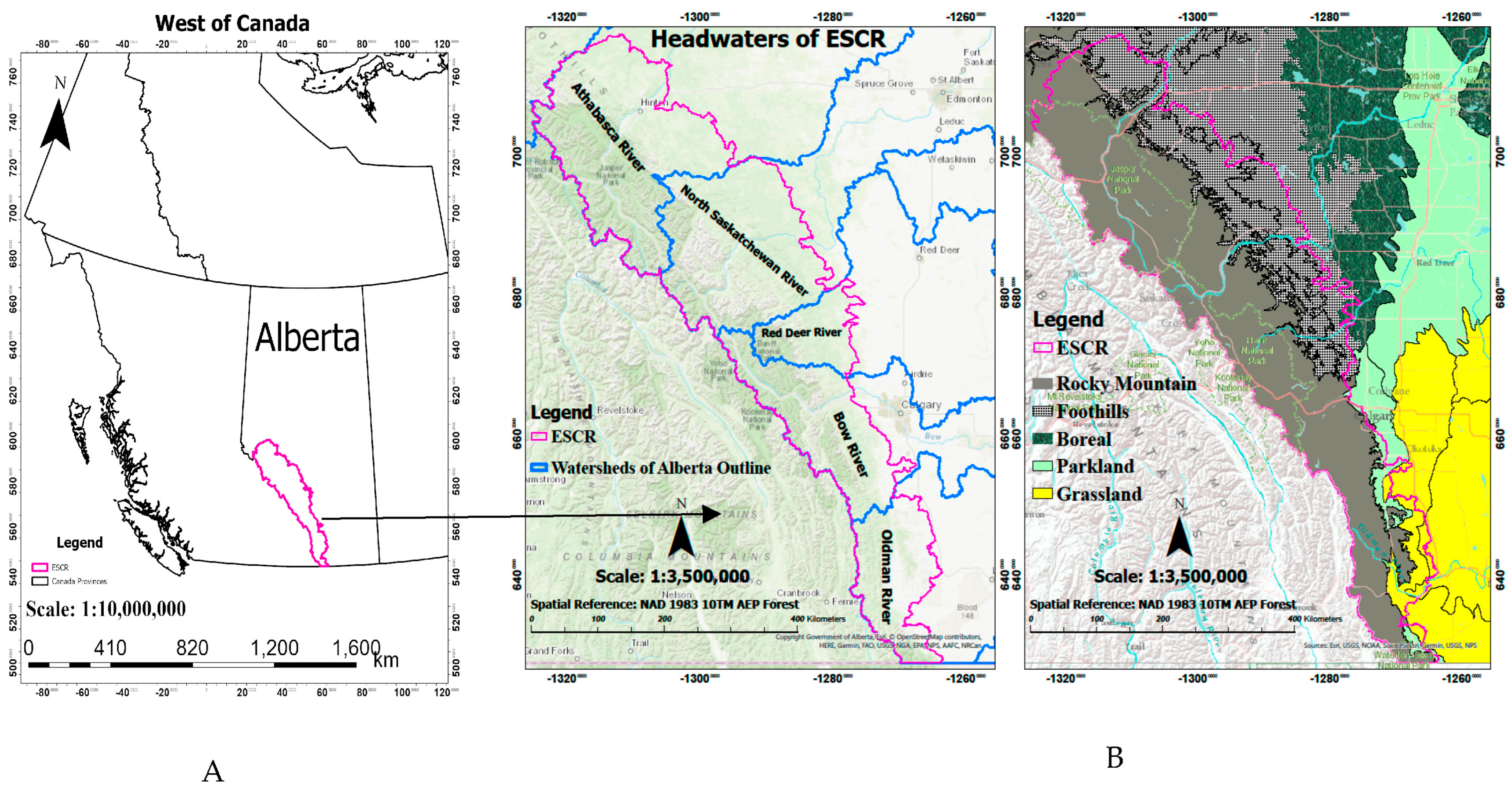
Figure 1. (A): Spatial extent and watershed boundaries of the ESCR, and (B): Natural regions and ecological zones.
Remotesensing 17 04004 g001
Figure 2. An illustration of the process of producing ATEI on GEE based on the NDVI and DEM.
Remotesensing 17 04004 g002
Figure 3. The diagram illustrates the Gaussian function of the second ATEI component (C2), and the distribution of unsmoothed maximum NDVI values of 386 randomly selected Landsat 8 pixels was analyzed to determine the normal distribution, the median, and the standard deviation of maximum NDVI values.
Remotesensing 17 04004 g003
Figure 4. Three main components of ATEI after standardization, (A): Abrupt spatial shift in NDVI (C1), (B): Gaussian function (C2), (C): Spatial covariation of NDVI and elevation (C3).
Remotesensing 17 04004 g004
Figure 5. The spatio-temporal distribution of ATE is displayed over nine composite periods (1984–2023) along the ESR. ATE extents have been calculated from the ATEI for the following periods: 1984–1989, 1990–1995, 1996–1998, 1999–2002, 2003–2006, 2007–2011, 2013–2015, 2016–2020, and 2021–2023. A black polygon represents the extent of ATE and is overlaid on natural-color Landsat imagery. This sequence illustrates the dynamics and movement of treeline ecotones over time, as well as the growth of patches and increased patch connectivity over time, particularly in the central and southern regions. In the final panel, where forests have encroached on alpine landscapes, an inset magnifies spatially concentrated localized changes and dynamics in ATE.
Remotesensing 17 04004 g005
Figure 6. Spatiotemporal distribution of ATE in ESCR (1984–2023).
Remotesensing 17 04004 g006
Figure 7. Over the years 1984–2023, variations in altitude (mean) of ATE are observed according to the different aspects of ESCR.
Remotesensing 17 04004 g007
Figure 8. Changes in ATE pixels in five watersheds.
Remotesensing 17 04004 g008
Table 1. The Mann–Kendall test with a 95% confidence level in ATE zone.
YearAspectTrendChanging Altitude (m)p-Value
1984–2023NNo+40.210.201
1984–2023NENo+18.210.28
1984–2023ENo+11.10.201
1984–2023SENo+8.50.088
1984–2023SNo+7.10.594
1984–2023SWNo+1.771
1984–2023WNo+3.910.74
1984–2023NWNo+27.120.166
Table 2. Spatial variation trend analysis of ATE in the different watersheds of the ESCR between 1984 and 2023.
WatershedMean of Watershed Elevation (a.s.l)Area (km2)Area (%)Increase
(km2)
No Change
(km2)
Decrease
(km2)
Total ChangeTotal Observedp-Value
Old Man1510.7411,377.1614.5366.0378.8743.57109.60188.470.1001
Bow1843.268883.6618.60246.30204.18169.45415.75619.930.0008
Red Deer1695.304825.367.8954.8633.3065.39120.25153.550.6306
North Saskatchewan1768.8917,027.2727.84258.58176.10221.98480.56656.660.2481
Athabasca1681.0419,038.4531.13262.71311.31189.23451.94763.250.0025
Disclaimer/Publisher’s Note: The statements, opinions and data contained in all publications are solely those of the individual author(s) and contributor(s) and not of MDPI and/or the editor(s). MDPI and/or the editor(s) disclaim responsibility for any injury to people or property resulting from any ideas, methods, instructions or products referred to in the content.