Data Augmentation and Interpolation Improves Machine Learning-Based Pasture Biomass Estimation from Sentinel-2 Imagery

Highlights

What are the main findings?

• Full-band Sentinel-2 reflectance combined with weather variables substantially improved pasture biomass prediction accuracy, outperforming vegetation indices and achieving up to 70% variance explained after interpolation.
• Multiquadric interpolation and progressive temporal training strengthened temporal consistency in the data, reducing prediction errors by approximately 30% relative to sparsely sampled baselines.

What are the implications of the main findings?

• These findings demonstrate that integrating physically meaningful spectral information with biologically constrained data augmentation enhances the reliability and scalability of satellite-based biomass estimation across farms and seasons.
• The resulting open-source modelling framework provides a robust foundation for real-time pasture monitoring and can be readily incorporated into automated decision-support tools for precision grazing management.

Abstract

Accurate pasture biomass (PB) estimation is critical for tactical grazing management, yet traditional satellite-derived vegetation indices such as Normalised Difference Vegetation Index (NDVI) saturate when canopy density exceeds about 3 t DM ha⁻¹. This limits predictive accuracy because the spectral signal plateaus under dense vegetation, masking further biomass increases. To address this limitation, this study integrated multiple data sources to improve PB estimation in dairy systems. The dataset combined Sentinel-2 spectral bands, rising plate-meter (RPM) PB measurements, daily weather data, and paddock management features. A total of 3161 paired RPM–satellite observations were collected from 80 paddocks across 16 New South Wales dairy farms between November 2021 and July 2024. Eight regression algorithms and four predictor configurations were evaluated using robust cross-validation, including an 80:20 farm/paddock-stratified train–test-set split. The XGBoost model using full-band reflectance and concurrent weather data achieved strong baseline performance (R² = 0.63; MAE = 243 kg DM ha⁻¹) on non-interpolated data, outperforming NDVI-based models. To address temporal gaps between field readings and satellite imagery, Multiquadric interpolation was applied to RPM data, adding roughly 30% new observations. This enhanced dataset improved test performance to R² = 0.70 and MAE = 216 kg DM ha⁻¹, with gains maintained on external validations (R² = 0.41/0.48; MAE = 267/235 kg DM ha⁻¹). A progressive training strategy, which refreshed model parameters with seasonally aligned data, further reduced errors by 30% compared to static models and sustained performance even when farms or seasons were excluded. This fortified Sentinel-2 modelling workflow, combining RPM interpolation and progressive calibration, achieved accuracy comparable to the commercial Pasture.io platform (R² = 0.66; MAE = 240 kg DM ha⁻¹) which uses satellite imagery with higher temporal and spatial resolution, demonstrating potential for automated recalibration and near real-time, paddock-level decision support in pasture-based dairy systems.

1. Introduction

Reliable estimation of above-ground pasture biomass or pasture biomass (PB) is essential for effective farm management, feed budgeting, and decision-making in pasture-based dairy systems. As global demand for agricultural efficiency grows, accurate and scalable PB monitoring tools become increasingly important. Pasture biomass estimation supports livestock system productivity, maintains environmental sustainability through optimised resource use, and improves economic viability across diverse farming operations [1]. However, conventional data collection methods like rising plate meters (RPM), a tool that relates compressed height of PB with the amount of biomass present, provide relatively high-quality data but are labour intensive, time consuming and impractical for daily monitoring, and this could create operational bottlenecks for farmers seeking to balance productivity with operational sustainability [2,3].

In contrast, satellite remote sensing provides broad scale, repeatable and comparatively low cost coverage of vegetation condition [1,4]. Yet, its most widely used proxy, the Normalised Difference Vegetation Index (NDVI), saturates under dense canopies, reducing sensitivity to PB and flattening response curves, which compromises predictive accuracy [5,6]. Alternative indices, including the Enhanced Vegetation Index (EVI), Soil-Adjusted Vegetation Index (SAVI) and Normalised Difference Red-Edge Index (NDRE), are derived from different combinations of spectral bands and offer only marginal improvements, unable to accurately predict PB on their own [7,8]. Because PB variability is driven by multiple factors such as soil moisture, paddock management, short-term weather extremes and region-specific sward composition, indices alone cannot explain PB variation; these additional drivers must be represented explicitly in modelling frameworks [9,10].

Sentinel-2 provides free, high-temporal and high-spatial resolution multispectral imagery that supports large-scale, frequent PB measurements, making it a cost-effective alternative relative to other options like UAV-mounted sensors, field spectrometers, and ground-based cameras [10,11,12,13]. Its diverse spectral bands allow researchers to monitor vegetation health and growth consistently and affordably [14,15].

However, satellite-based data utilisation has its inherent limitations [16]. Cloud cover, atmospheric interference and inclement weather conditions can produce unreliable satellite-derived products or no data at all, limiting PB estimates for decision-making using this approach and reducing reliable insights on pasture management and utilisation [4,8]. On days when satellite data are completely unavailable, for example on cloudy or snowy days, ground-based RPM measurements are usually employed to compensate for missing satellite data to maintain consistent flow of data [9,10,17,18].

Integrating diverse data sources offers a potential solution to these challenges. Recent research shows that combining raw satellite imagery with ground-truth measurements, weather variables and paddock-specific information, can significantly enhance PB prediction accuracy [10,18]. Machine learning (ML) algorithms such as Random Forests (RF), Support Vector Machines (SVM) and Artificial Neural Networks (ANN) have been used in these integrations and outperform traditional regression methods and linear programming by providing better insights, identifying nonlinear relationships between driving factors affecting pasture growth and managing high-dimensional data, and adapting to temporal and spatial variability, thereby offering a more comprehensive understanding of pasture utilisation and management [19,20,21,22].

As an alternative or complement to ML approaches, physiological growth models provide mechanistic insights into pasture dynamics by simulating processes such as photosynthesis, respiration, and nutrient uptake based on environmental drivers. Models such as DairyMod, APSIM-Pasture, and ModVege have been successfully applied to predict pasture growth in temperate grazing systems, offering interpretable predictions grounded in plant ecophysiology [23,24,25,26]. While these process-based models excel at capturing temporal growth patterns under varying environmental conditions, they typically require extensive parameterisation and may lack the flexibility to incorporate high-dimensional remote sensing data directly [27]. Hybrid approaches that combine the mechanistic foundation of physiological models with the pattern-recognition capabilities of ML algorithms represent a promising research direction, potentially leveraging the strengths of both methodologies to improve predictive accuracy and model interpretability [28,29].

However, significant research gaps persist, particularly regarding temporal and spatial misalignments between satellite data and ground measurements, which create inconsistencies as satellite observations often do not coincide with the timing or location of ground data collection. Furthermore, missing data due to cloud cover or other environmental obstructions disrupts the continuity of satellite-derived datasets [4,30]. Addressing these issues requires sophisticated data manipulation strategies such as interpolation techniques to fill gaps, synthetic data generation to expand datasets and progressive training to capture temporal patterns across different scenarios [31]. The generalisability of models across regions and farming systems is also a concern as a model trained on data from one area or region may perform well within that context, however, its applicability to other areas or locations with different weather, soil, and management conditions is not guaranteed. Therefore, evaluating reliability and flexibility using external validation datasets is essential to ensure that the predictive framework is not overly tailored to a specific environment but remains versatile enough for broader adoption.

Building on these challenges highlighted, this research poses several key questions to address the limitations of current pasture estimation methods. First, how can the integration of raw satellite imagery, RPM measurements, weather data, and paddock-specific characteristics significantly enhance PB prediction accuracy, especially overcoming the known saturation issues of conventional derived vegetation indices like NDVI? Second, how effectively can the integration of diverse data sources address the challenges of missing or unreliable satellite readings caused by cloud cover, thereby ensuring data continuity for robust model performance? Third, can advanced ML models effectively compensate for temporal and spatial mismatches, ensuring their validity and reliability when applied to external datasets across varied weather, soil, and management contexts, thereby offering a robust and generalisable solution beyond existing site-specific approaches?

To address these questions, the objectives of this study are threefold. First, to develop an integrated ML framework that leverages raw Sentinel-2 reflectance, RPM-derived PB, weather, and paddock management characteristics to accurately estimate PB. Second, to evaluate the reliability and transferability of the framework across diverse temporal and spatial conditions, including unseen farms and seasons, by leveraging data augmentation and progressive training strategies. Third, to benchmark the developed framework against a commercial platform, demonstrating its practical application as a transparent, cost-effective and scalable solution for sustainable near real-time, farm-specific pasture utilisation and management in dairy systems.

2. Materials and Methods

2.1. Study Area and Data Sources

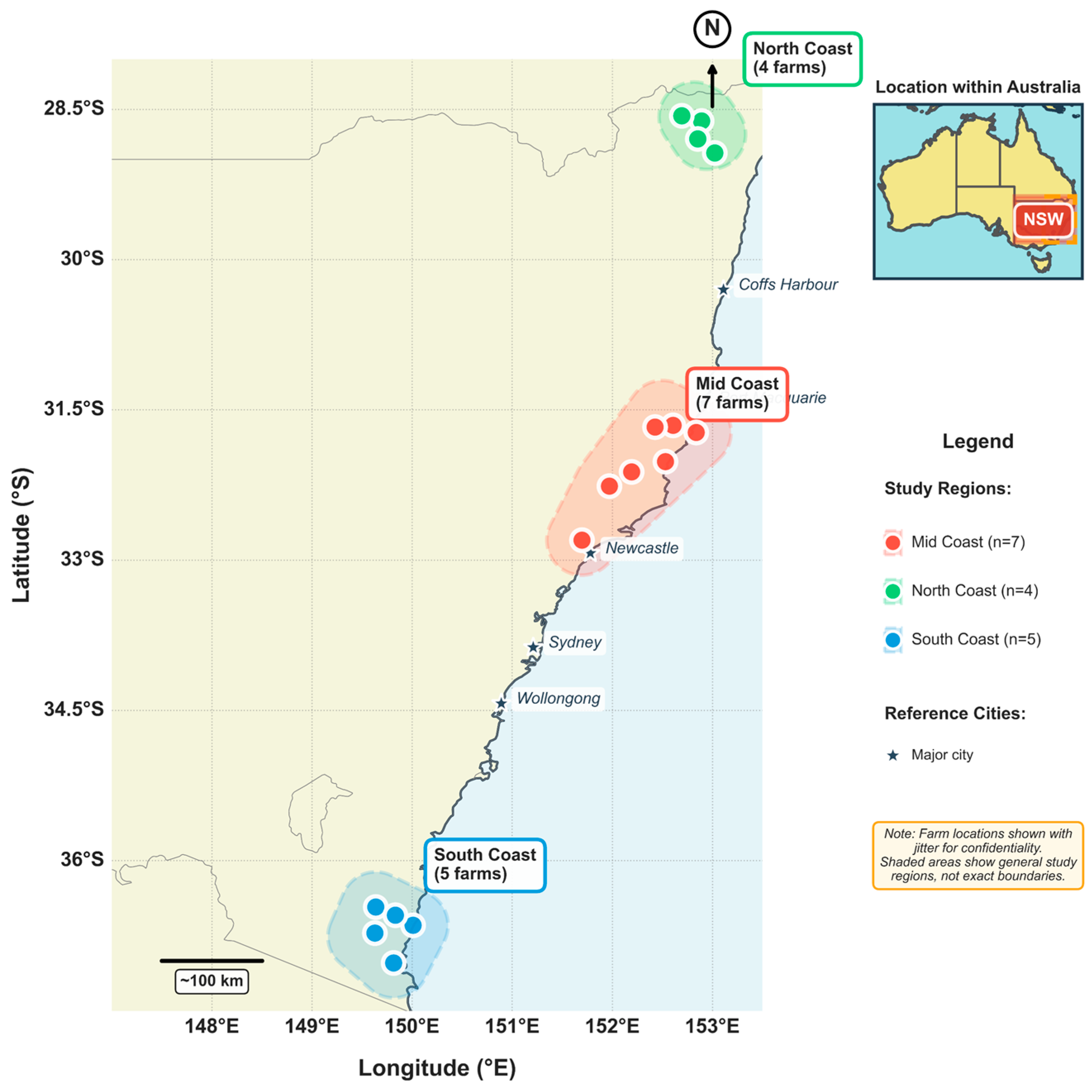
This study was conducted across 16 commercial dairy farms located in three coastal districts of New South Wales (NSW), Australia, between November 2021 and July 2024 (Figure 1). The farms were distributed across the mid-coast district (n = 7 farms, latitude range: −34.03° to −31.72°S, longitude range: 150.65° to 152.68°E), the south coast (n = 5 farms, latitude range: −36.82° to −36.64°S, longitude range: 149.60° to 149.90°E), and the north coast (n = 4 farms, latitude range: −28.90° to −28.68°S, longitude range: 152.91° to 153.13°E), with specific farm coordinates withheld to maintain commercial confidentiality. These farms collectively managed 2436 hectares of grazing land, with herd sizes varying from 105 to 580 milking cows, and individual farms containing between 22 and 83 paddocks, with utilisable grazing areas ranging from 64.5 ha to 313 ha. The study regions presented diverse weather conditions, with long-term mean annual rainfall averaging approximately 780 mm in the south coast, 1284 mm in the mid-coast, and 1073 mm in the north coast. Average daily air temperatures ranged from approximately 5 to 20 °C in winter and 20 to 35 °C in summer. All farms had pastures based on kikuyu (Cenchrus clandestinus, previous Pennisetum clandestinum), which produces biomass from late spring (November) through summer and autumn, oversown every year (March to April) with annual ryegrass (Lolium multiflorum L.), which produces biomass during autumn, winter, and early spring.

Remote sensing data was acquired from Copernicus Sentinel-2 surface reflectance imagery, which offers 10 m spatial resolution and a nominal five-day revisit cycle for each paddock in each farm during clear-sky passes. The spectral bands retained for analysis included blue, green, red, near-infrared, red-edge 1 to 3, and short-wave infrared 2 and 3. Standard vegetation indices such as NDVI, EVI, SAVI, and NDRE were also calculated per pixel. To ensure data quality, pixels were masked using the Function of mask (Fmask) layer, classifying them as valid, water, cloud, shadow, or snow.

Ground-truth PB measurements were conducted using an RPM. A Jenquip EC20 Electronic Pasture Meter (Feilding, New Zealand) was specifically utilised to obtain Compressed Sward Height (CSH) readings. Five primary paddocks on each farm were selected for continuous monitoring over the two-year study period (November 2021 to July 2024), along with one additional reserve paddock (the sixth paddock) which served as a spatially independent validation site. The selection of these five primary paddocks was based on the following criteria: (i) representativeness of the predominant pasture species composition on each farm (kikuyu oversown with annual ryegrass), (ii) accessibility for consistent fortnightly/weekly sampling throughout the study period, (iii) diversity in paddock size and topographic characteristics to capture farm-level variability, and (iv) active incorporation in the farm’s regular grazing rotation to ensure realistic management conditions. The sixth paddock was intentionally withheld from model training to provide an independent spatial validation dataset, representing genuine out-of-sample conditions for assessing model generalisation to unseen paddock locations within the same farm.

RPM calibration was an integral part of the data collection, performed monthly on two designated fixed paddocks per farm [10]. The calibration process involved collecting nine 0.1 m² quadrat cuts at a 5 cm stubble height, stratified across the paddock to capture high, medium, and low biomass zones (three cuts per zone). Samples were dried for 48 hours at 65 °C, weighed, and subsequently regressed against the corresponding CSH measurements to derive farm-specific and seasonally adjusted conversion equations. This approach ensured that CSH-to-PB conversions accounted for seasonal changes in pasture density and species composition. The monthly calibration frequency was designed to capture phenological changes in sward structure that could affect the CSH-PB relationship, particularly during transitions between kikuyu and ryegrass dominance. This process allowed for the accurate conversion of CSH readings into PB, expressed as kilograms of Dry Matter per hectare (kg DM ha⁻¹). For each paddock, a minimum of 70 plate measurements were recorded and then converted to PB in kg DM ha⁻¹ [10,18]. The spatial distribution of measurements within each paddock ensured that areas with varying slope, drainage, and proximity to high-traffic zones (gates, water points, shade structures) were adequately represented, thereby minimising bias from localised management effects or microtopographic variation.

Additionally, environmental data consisting of daily weather variables for each farm were obtained from the SILO Long Paddock platform (https://www.longpaddock.qld.gov.au). Variables used were maximum air temperature (°C), minimum air temperature (°C), rainfall (mm), vapour pressure (kPa), maximum and minimum relative humidity (%), incoming solar radiation (MJ m⁻²) and evapotranspiration (mm). These observations were obtained to provide essential information regarding weather influences on PB.

2.2. Data Preprocessing

Sentinel-2 images were corrected to surface reflectance, resampled to a common 10 m grid and clipped to paddock boundaries obtained from the georeferenced GIS dataset for each farm. The pixel-quality layer Fmask [32] classified each pixel as valid, water, cloud, shadow or snow, and only pixels flagged valid were retained for analysis. For every monitored paddock on the day an image was taken, the mean reflectance of blue, green, red, near-infrared, red-edge 1-3 and short-wave-infrared 2-3 was calculated, and vegetation indices NDVI, EVI, SAVI and NDRE were derived. Spectral outliers falling outside 1.5 interquartile ranges from the first or third quartile were removed before averaging.

Rising plate-meter records were filtered to keep PB between 1000 kg DM ha⁻¹ and 4000 kg DM ha⁻¹. Approximately 70 individual RPM readings collected within each paddock on a monitoring day were averaged to one PB value per paddock. Within each farm-paddock-date group, categorical fields such as paddock name were reduced to their modal value and numeric fields were averaged. Daily SILO weather data were converted to numeric, checked for implausible entries and merged directly by each farm and calendar date.

Date stamps in every dataset were converted to datetime and expanded to ISO week number, calendar year and austral seasons, where Spring includes September to November, Summer (December to February), Autumn (March to May) and Winter (June to August). Satellite data, daily weather observations and PB estimates were merged on farm code, paddock code and date. When Sentinel and plate-meter observations were not recorded on the same day, PB rows were retained only if a Sentinel acquisition occurred within ±3days. Rows with missing predictor values were removed on a complete-case basis, and continuous variables were centred and scaled to unit variance for subsequent modelling, yielding a curated dataset of 3161 records from 80 paddocks across the 16 farms.

2.3. Interpolation Methods for Data Augmentation

Following the merging of the RPM measurements, collected weekly in year 1 and fortnightly in year 2, with Sentinel-2 passes that recur on an approximately five-day revisit cycle, small temporal gaps remained in PB because satellite imagery does not provide a direct PB measurement from the bands. To expand the dataset, these gaps were filled within each paddock in each farm using stochastic interpolation routines implemented in Python (v3.11.4).

Four interpolation techniques were assessed to augment PB observations for the merged dataset (RPM and Sentinel). The set comprised a second order polynomial in time as the baseline curve, a Gaussian radial basis function, a multiquadric radial basis function [33,34] and a minimum curvature exact spline. Radial basis surfaces offered flexible data-driven alternatives that perform well for smooth, yet non-linear environmental series [35,36,37] and the minimum curvature spline minimises the surface Laplacian, a property valued in geophysical analysis [38]. All four algorithms were executed independently three times for each paddock in each farm: once on year 1 data only (dates earlier than 1 April 2023), once on year 2 data only (dates on or after 1 April 2023) and once on the combined two-year record to exploit longer term temporal structure where available.

Interpolation was performed only when at least three actual PB observations were available for a paddock and was strictly confined to the temporal span defined by those observations, thereby preventing any extrapolation. Analysis of observation intervals revealed that time gaps between consecutive pasture meter measurements in the final dataset ranged from 7 to 14 days (median = 7 days, mean = 8.4 days). The majority of intervals (84.9%) were ≤14 days, with 94.3% ≤30 days and only 1.6% exceeding 60 days. The multiquadric radial basis function employed is appropriate for capturing smooth temporal trajectories across such intervals, as pasture growth follows gradual, predictable patterns between discrete grazing events rather than exhibiting abrupt discontinuities. For the small proportion of longer intervals (>60 days), interpolation remained constrained to the temporal span of observed measurements, with no extrapolation beyond the empirical record. All time stamps were converted to Unix epoch seconds to provide a uniform, monotonic reference axis for curve fitting. Prior to modelling, any PB measurement falling outside the biologically credible interval of 1000 to 4000 kg DM ha⁻¹ was discarded. After the gap-filling procedure each record was annotated to indicate whether Sentinel-2 reflectance originated from a nearest-date substitution and whether the corresponding PB simulated was replaced by an interpolated value, enabling downstream analyses to distinguish directly measured data from synthetically generated values. Rows with null values after processing were discarded. The combination of biological filtering, nearest-date filling and advanced interpolation produced a comprehensive temporal gap-free dataset containing 9816 daily records from 80 paddocks across the 16 farms.

2.4. Predictive Modelling for Pasture Biomass

2.4.1. Model Training and Optimisation

Univariate analysis was employed to quantify linear relationships between each predictor and the response variable PB (kg DM ha⁻¹) using a Pearson correlation matrix visualised as a heat map. Numerical predictors comprised daily maximum temperature (°C), daily minimum temperature (°C), evapotranspiration (mm d⁻¹), incoming solar radiation (MJ m⁻² d⁻¹), vapour pressure (kPa), rainfall (mm d⁻¹), maximum and minimum relative humidity (%), ten (10) Sentinel-2 spectral bands (blue, green, red, near infra-red, red edge 1 to 3, short-wave infra-red 2 and 3) and four derived vegetation indices (NDVI, SAVI, EVI, NDRE). While standard greenness indices (NDVI, EVI, SAVI, NDRE) were calculated, SWIR-based indices such as the Cellulose Absorption Index (CAI) were not explicitly derived, as the tree-based ML algorithms were expected to capture relevant SWIR band information through non-linear feature interactions. Categorical predictors were season, coastal region and grazing information; these were examined with box plots and frequency tables. Four feature sets were defined: (i) all bands with indices, (ii) all bands with weather data and indices, (iii) bands only and (iv) bands with weather data without indices. These configurations were assessed to determine which combination of variables most effectively models PB and to quantify the contribution of weather and vegetation indices to its variability. Predictors showing negligible correlation or high collinearity were removed.

All analyses in this study were carried out in Python (v3.11.4). Categorical variables were one-hot encoded and numerical features were centred and scaled with StandardScaler. Data were split randomly into training and test partitions at an 80:20 ratio, after which multiple random seeds were evaluated through a five-fold three-repeat Repeated K-Fold cross-validation loop to stabilise estimates. Eight regression algorithms, linear regression (LR), least absolute shrinkage and selection operator (LASSO), decision tree (DT), support vector regression (SVR), k-nearest neighbours (KNN), random forest (RF), gradient boosting machine (GBM) and extreme gradient boosting (XGBoost), were wrapped in scikit-learn pipelines. Hyper-parameters for every algorithm were declared in a single Python dictionary; tree ensembles varied the number of decision trees (n_estimators) from 50 to 450 and maximum depth from 3 to 10, while SVR varied the cost regularisation parameter C from 0.1 to 10 and kernel type. A grid search procedure was employed to systematically test all hyper-parameter combinations, selecting the configuration that minimised negative mean absolute error (MAE, kg DM ha⁻¹), and the model with the lowest cross-validated error was retained.

2.4.2. Progressive Training for Temporal Consistency

To examine how sequential retraining influences model performance while preserving the chronological order of new observations, a progressive training strategy developed by Correa-Luna, et al. [10] was adopted. Every record carried calendar year, month, ISO week, and week of month (WOM), enabling four nested training subsets that represented 25%, 50%, 75% and 100% of each monthly cycle. The subsets were defined as follows: 1 W used WOM = 1; 2 W used WOM = 1 or 2; 3 W used WOM = 1, 2 or 3; and 4 W used WOM = 1, 2, 3 or 4. After each increment, the best model was refitted on the enlarged subset and evaluated on the unchanged test split, with MAE retained as the optimisation metric. The protocol was run separately on the non-interpolated dataset and on the interpolated dataset created in Section 2.3, ensuring that temporal consistency was assessed under both raw and augmented conditions without introducing look-ahead bias. Additionally, to assess inter-annual generalisation, an additional experiment trained the model onYear1Set (data collected before 1 April 2023) and evaluated it on Year2Set (data collected on or after that date), using three dataset variants: the non-interpolated data, a Year 1 multiquadric-interpolated dataset and a full-period multiquadric-interpolated dataset.

2.4.3. Pasture Biomass Model Validation

For the validation, two independent hold-out samples were excluded from all training steps, including non-interpolated, interpolated, and progressive training workflows, and were kept free of any interpolation or gap-filling procedures to represent truly unseen data. The first independent validation sample comprised 41 records representing all available and valid paired RPM PB and Sentinel-2 imagery observations collected from the five primary monitored paddocks across nine of the study farms between 1 and 30 November 2024. The specific count of 41 records was the outcome of applying the data-quality filters (i.e., PB values between 1000 and 4000 kg DM ha⁻¹) to all available measurements during this validation period. For these records, PB measured with RPM was merged with same-day Sentinel-2 imagery, and cloud-affected scenes were handled by replacing them with the corresponding weekly mean reflectance. The selection of these nine farms was based on the availability of complete, high-quality independent data that met the validation criteria during this specific November 2024 period, ensuring they provided fresh, untainted observations.

The second independent validation sample consisted of 63 records reflecting all valid observations gathered specifically from the sixth monitored paddock on each participating farm for the whole period. This “sixth paddock” was intentionally designated as an additional, spatially distinct unseen geographic validation set. The 63 records represent the total number of valid observations obtained after applying the identical merging procedure and the same 1000–4000 kg DM ha⁻¹ PB filtering as the training data, ensuring comparable data quality while maintaining their independence. The predictive accuracy of the models on these truly independent datasets was quantified using standard performance metrics: root mean squared error (RMSE), mean absolute error (MAE), mean squared error (MSE), and the coefficient of determination (R²). These metrics were calculated separately for each independent hold-out sample, thereby enabling a robust assessment of the ability of the model to generalise to completely unseen, non-interpolated data across different temporal and spatial contexts.

3. Results

3.1. Dataset Overview and Exploratory Analysis

Descriptive analysis of the final curated non-interpolated paired RPM and Sentinel-2 dataset (3161 observations) resulted in a mean CSH of 80.2 ± 18.1 mm, an average PB of 2690 ± 503 kg DM ha⁻¹, with environmental drivers including daily maximum temperature of 23.7 ± 5.3 °C, rainfall averaging 1.7 ± 7.3 mm d⁻¹, and a mean NDVI of 0.72 ± 0.12 (

Table 1. Descriptive statistics for pasture, weather, and spectral variables (n = 3161) used in the study.

Variables	Min.	25%	Median	Mean	75%	Max.	SD
Compressed Height (mm)	24.68	68.02	81.81	80.20	94.45	145.00	18.06
Pasture Biomass (kg DM ha−1)	1153.33	2352.08	2737.85	2690.20	3087.74	3720.00	503.06
Daily Max. Temperature (°C)	11.00	19.60	23.30	23.73	27.60	43.00	5.26
Daily Min. Temperature (°C)	−1.10	6.50	11.10	10.97	15.60	27.10	5.66
Rainfall (mm day−1)	0.00	0.00	0.00	1.70	0.30	115.20	7.27
Evapotranspiration (mm day−1)	0.00	2.10	3.50	3.91	5.40	10.80	2.21
Solar Radiation (MJ m−2 day−1 )	2.90	11.40	14.70	16.46	21.40	31.80	6.80
Vapour Pressure (kPa)	5.40	10.80	14.20	15.20	19.10	29.80	5.33
Max. Relative Humidity (%)	19.40	42.40	49.10	50.33	56.80	93.20	11.87
Min. Relative Humidity (%)	43.70	100.00	100.00	96.77	100.00	100.00	8.22
Blue Band Reflectance	204.91	355.06	421.72	446.73	515.01	836.00	124.39
Green Band Reflectance	379.00	654.69	716.94	735.07	804.70	1117.50	114.56
Red Band Reflectance	214.83	406.97	518.76	564.23	675.00	1307.17	205.89
NIR Band Reflectance	1024.00	3248.95	3758.85	3730.16	4247.21	5996.74	780.05
Red-Edge 1 Reflectance	514.90	986.59	1096.48	1130.08	1257.62	1789.98	214.68
Red-Edge 2 Reflectance	999.93	2554.54	2871.03	2875.78	3231.93	4475.48	544.21
Red-Edge 3 Reflectance	965.17	3010.53	3491.91	3485.73	3987.18	5744.56	739.27
SWIR-2 Reflectance	779.00	1888.85	2112.62	2167.65	2420.06	3478.27	442.39
SWIR-3 Reflectance	327.00	880.23	1028.72	1099.93	1266.77	2200.18	314.58
NDVI	0.27	0.66	0.75	0.72	0.82	0.92	0.12
EVI	0.10	0.47	0.59	0.57	0.69	1.01	0.15
SAVI	0.10	0.43	0.52	0.50	0.59	0.75	0.11
NDRE	0.12	0.45	0.54	0.52	0.60	0.74	0.11

Min. = minimum; 25% and 75% = first and third quartiles; Max. = maximum; SD = standard deviation.

). Average PB values exhibited marked seasonal and regional variation across all farms, peaking in summer at approximately 2900 kg DM ha⁻¹ and declining to around 2526 kg DM ha⁻¹ in winter, representing a 15% amplitude primarily driven by radiation and temperature rather than instantaneous rainfall. Mid-coast paddocks averaged 2830 kg DM ha⁻¹, the south coast 2644 kg DM ha⁻¹, and the north coast 2582 kg DM ha⁻¹.

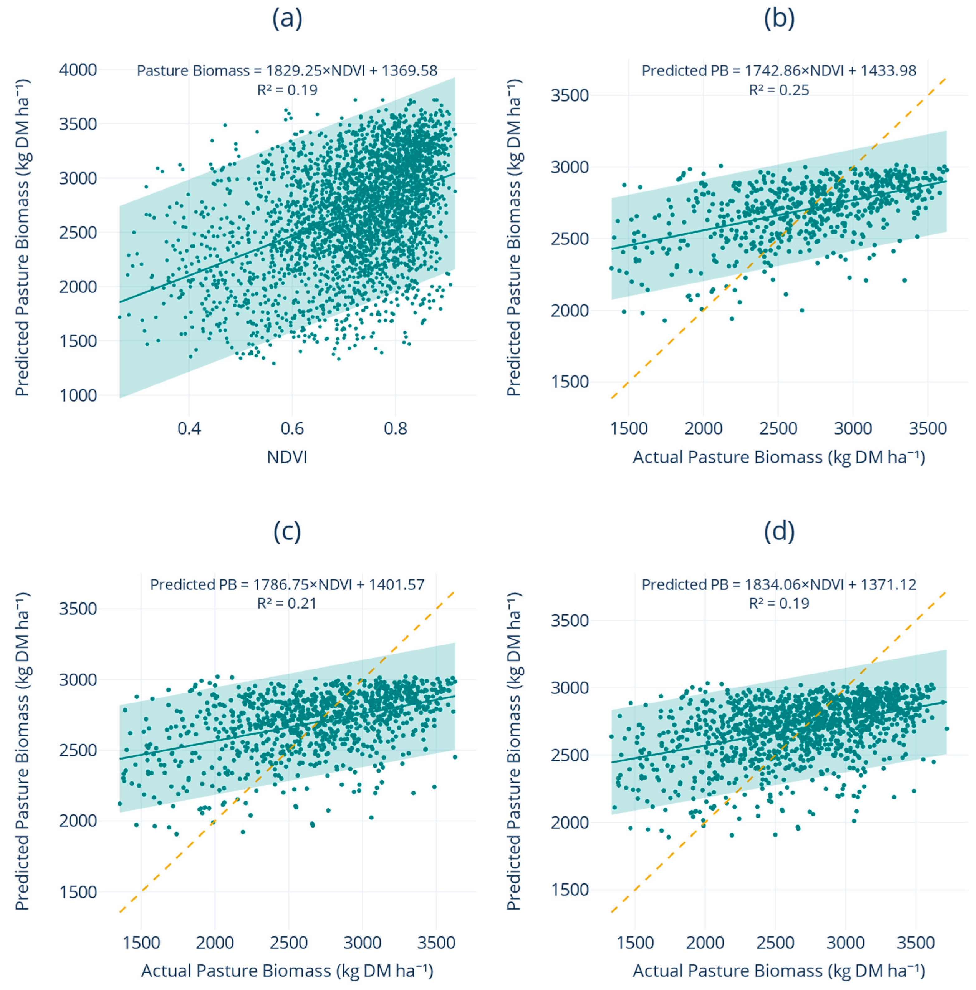
Greenness saturation is evident in Figure 2 below. A second-order polynomial regression of NDVI against PB across the entire dataset revealed a non-linear relationship with R² = 0.20 (Figure 2a), clearly demonstrating the saturation of NDVI at high biomass levels where the index plateaus while PB continues to increase, and progressively larger test splits (80:20, 70:30, 60:40; Figure 2b–d) retain similar slopes and R² values (0.20–0.25). The fan-shaped residual pattern shows that NDVI plateaus near 0.80 while PB continues to rise beyond 3000 kg DM ha⁻¹, with NDRE emerging as the sole significant positive coefficient (+3701 kg DM ha⁻¹ unit⁻¹, p < 0.001).

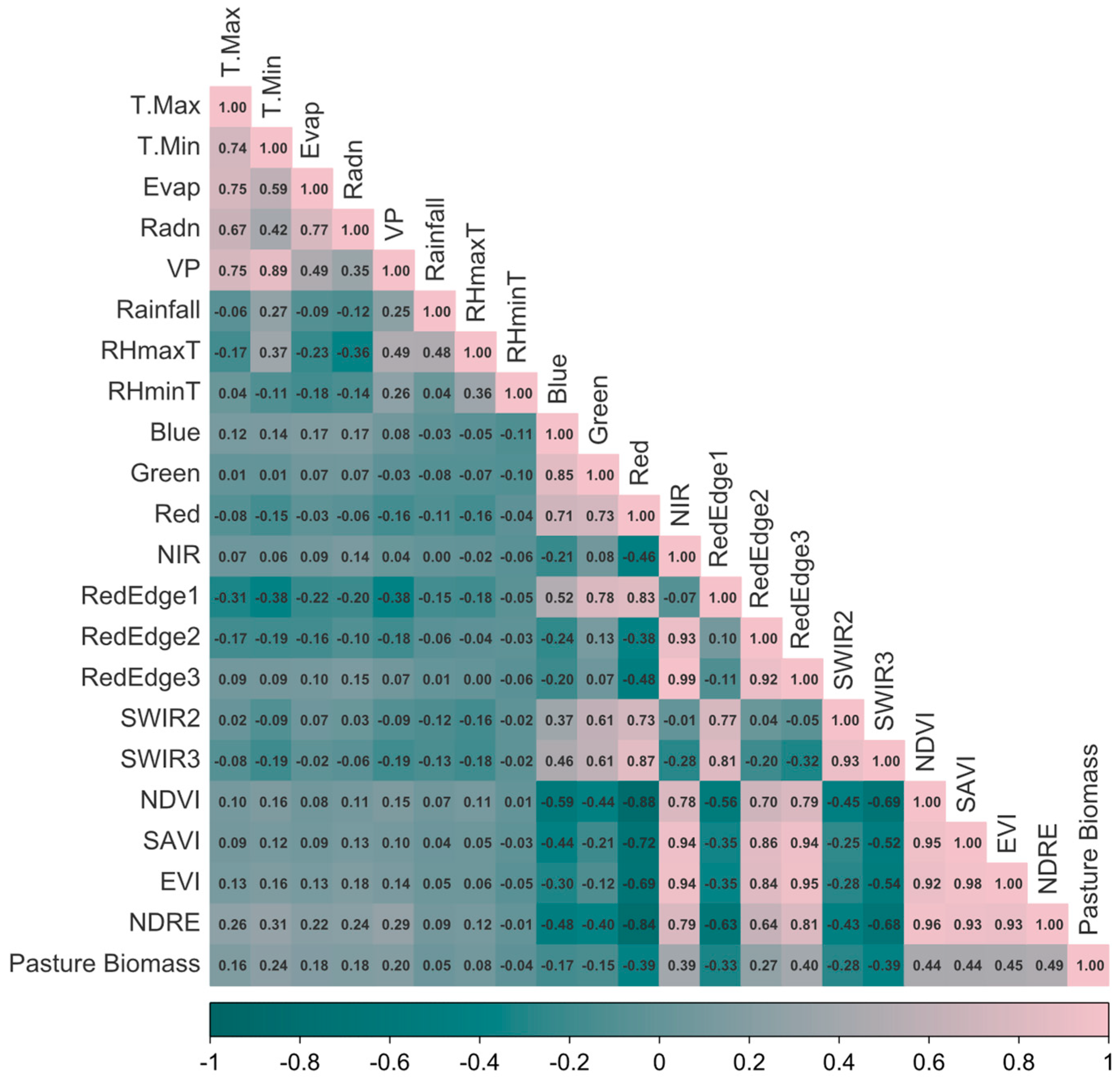
Inter-variable relationships, visualised in the Pearson-correlation heat map (Figure 3), partitioned predictors into three main clusters. First, the ten Sentinel-2 bands are highly auto-correlated (r > 0.70), a redundancy that later justifies dimensional reduction or tree-based feature selection. Second, the greenness–biomass cluster shows positive correlations between PB and composite indices, namely NDRE (r = 0.49), EVI (0.45), NDVI (0.44), and SAVI (0.44), and negative correlations with red and SWIR reflectance (r −0.39), reflecting the classical red–NIR contrast and water-absorption effects. Third, the weather cluster revealed tight coupling among maximum temperature, evapotranspiration, and solar radiation (r ≈ 0.75), but only weak instantaneous ties to PB (r ≤ 0.18). The five strongest positive and negative coefficients highlight the immediate value of red-edge indices, with NDRE and EVI as the most informative single predictors, whereas high-wavelength reflectance exerts the strongest damping influence.

3.2. Baseline Model Development and Predictive Accuracy

Eight regression algorithms were benchmarked on the non-interpolated dataset under four predictor configurations that varied the presence of weather variables and vegetation indices. Each pipeline applied one-hot encoding to categorical features, standard scaling to numeric features, and underwent hyper-parameter tuning via a five-fold, three-repeat Repeated K-Fold search that minimised MAE (Section 2.4.1). An 80:20 random split (n = 2528 training set, 633 test set) provided an unseen test set, while two independent hold-out samples supplied geographic and temporal validation.

Table 2. Test-set and cross-validation performance of the eight regression algorithms all using Sentinel-2 bands and weather variables (no vegetation indices).

Model	CV Score	MSE	RMSE	MAE	R2
Decision Tree	−336.38	168,853.56	410.92	331.35	0.37
Support Vector Regression	−289.99	138,196.95	371.75	289.81	0.48
Linear Regression	−284.00	129,687.39	360.12	285.11	0.51
Lasso Regression	−283.89	129,417.34	359.75	284.98	0.52
K-Nearest Neighbours	−283.06	126,959.97	356.31	281.89	0.52
Random Forest	−274.80	105,868.82	325.37	259.31	0.60
Gradient Boosting Machines	−249.08	105,539.33	324.87	252.70	0.60
Extreme Boosting Regressor	−246.41	98,036.41	313.11	243.12	0.63

CV Score is the negative mean absolute error (MAE) averaged across a five-fold, three-repeat cross-validation; MSE = mean squared error, RMSE = root mean squared error, and MAE (all in kg DM ha⁻¹); R² is the coefficient of determination on the independent 20% test split (n = 633). Extreme Boosting Regressor (XGBoost) records the lowest error metrics, underscoring the advantage of tree-ensemble methods for modelling PB from high-dimensional spectral and weather data.

summarises test-set results for the configuration that proved most dependable comprising all Sentinel-2 spectral bands combined with concurrent weather predictors but excluding vegetation indices. Within this setting, XGBoost achieved the lowest test error of all pipelines (RMSE = 313 kg DM ha⁻¹, MAE = 243 kg DM ha⁻¹, R² = 0.63) and the highest cross-validated score (CV MAE = 246 kg DM ha⁻¹). To demonstrate the value of integrating full spectral information, XGBoost performance was compared against NDVI-based approaches: when trained using NDVI alone, performance was substantially lower (RMSE = 439 kg DM ha⁻¹, MAE = 359 kg DM ha⁻¹, R² = 0.28), while combining NDVI with weather factors improved results (RMSE = 363 kg DM ha⁻¹, MAE = 284 kg DM ha⁻¹, R² = 0.50) but still underperformed regarding the full spectral approach by 41 kg DM ha⁻¹ in MAE and 13 percentage points in R². Random forest and gradient boosting models followed closely (MAE ≈ 260 kg DM ha⁻¹, R² ≈ 0.60), whereas linear, k-nearest-neighbour, and support vector regressions lagged by 40–50 kg DM ha⁻¹. Stand-alone decision trees performed worst with MAE = 331 kg DM ha⁻¹ and R² = 0.37, highlighting the stabilising value of ensemble averaging in a feature space dominated by collinear reflectance bands.

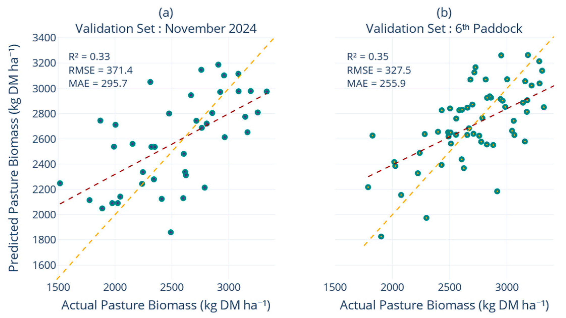
Figure 4 shows the association between actual and predicted PB on the non-interpolated test set for four predictor scenarios. Including the four derived indices (NDVI, SAVI, EVI, NDRE) lowered the XGBoost test-set MAE marginally from 243 to 238 kg DM ha⁻¹ and nudged R² to 0.65 (Figure 4b), yet this apparent gain disappeared on both validation sets. For the November 2024 paddocks, the index-rich model returned MAE = 315 kg DM ha⁻¹ and R² = 0.27, whereas the index-free model achieved MAE = 296 kg DM ha⁻¹ and R² = 0.33 (Figure 5a). A similar pattern emerged on the sixth-paddock sample (MAE = 264 versus 256 kg DM ha⁻¹, R² = 0.29 versus 0.35; Figure 5b).

Predictor sets that omitted either weather data or indices performed consistently worse (Figure 4a,c). Removing meteorological inputs lowered test-set R² by 5–6 points and raised MAE by roughly 30 kg DM ha⁻¹. Validation errors exceeded test errors by about 10%, and the ranking of model quality remained unchanged, with XGBoost ahead of GBM and RF, followed by linear methods. XGBoost presented test-set MAE 12% lower relative to linear regression and maintained that margin on both external validation datasets.

3.3. Effects of Feature Engineering and Data Augmentation

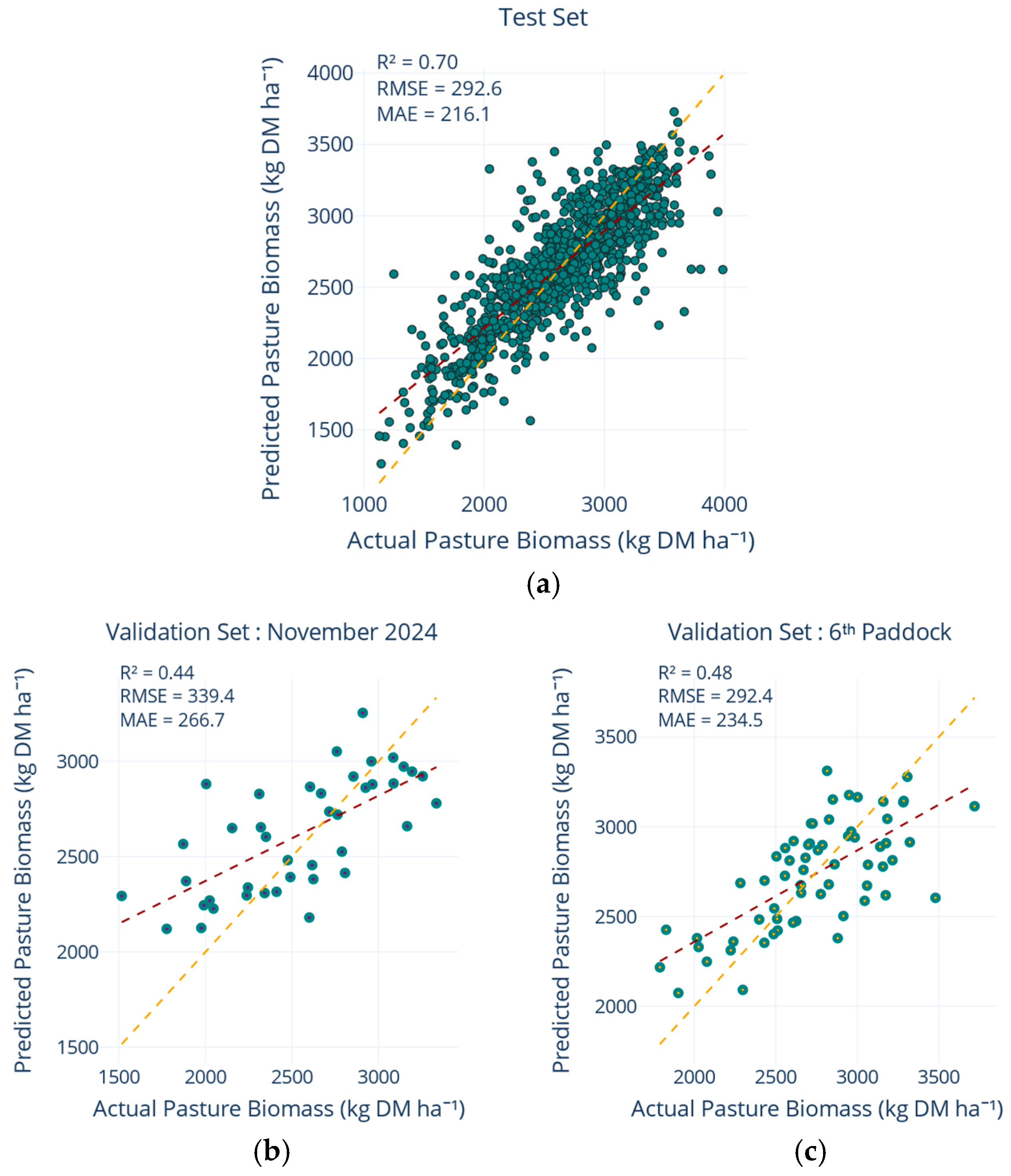
Interpolation of field measurements using four techniques, second-order polynomial, Gaussian radial-basis function (rbf), multiquadric radial-basis function (mq), and minimum-curvature spline (mcg), were applied under three scenarios as shown in Figure 5: Year1Set only, Year2Set only, or the combined dataset. These methods were benchmarked against the non-interpolated (Non_ip) baseline to assess their impact on model performance. Each experiment utilised the “All Bands with Weather Data without Indices” feature set and the XGBoost pipeline detailed in Table 2. Performance was evaluated using MSE, RMSE, MAE, and R² on the 80:20 test split and two independent hold-out validation sets, as defined in Section 2.4.3. A comparative analysis of these methods is presented in Figure 5. The results revealed that mq interpolation produced the most substantial improvements on the 80:20 test split. Augmenting the training data with approximately 30 per cent synthetic mq-derived observations increased the test R² from 0.63 to 0.70 and reduced the MAE from 243 to 216 kg DM ha⁻¹, an 11% improvement over the baseline. A parallel evaluation using the mq-interpolated dataset (

Table 3. Test-set and cross-validation performance of the eight regression algorithms using the mq-interpolated dataset under the “All Bands with Weather Data without Indices” feature configuration.

Model	CV Score	MSE	RMSE	MAE	R2
Decision Tree	−324.31	190,801.32	436.81	308.96	0.33
Support Vector Regression	−310.76	173,507.53	416.54	322.48	0.39
Linear Regression	−308.63	171,153.62	413.71	325.34	0.40
Lasso Regression	−308.63	171,145.21	413.70	325.34	0.40
K-Nearest Neighbours	−261.54	122,847.55	350.50	253.14	0.57
Random Forest	−246.65	100,377.68	316.82	237.21	0.65
Gradient Boosting Machines	−233.05	87,026.31	295.00	218.05	0.70
Extreme Boosting Regressor	−231.89	85,631.65	292.63	216.13	0.70

CV Score is the negative mean absolute error (MAE) averaged across a five-fold, three-repeat cross-validation; MSE = mean squared error, RMSE = root mean squared error, and MAE (all in kg DM ha⁻¹); R² is the coefficient of determination on the independent 20% interpolated test split (n = 982). Extreme Boosting Regressor (XGBoost) records the lowest error metrics, underscoring the advantage of tree-ensemble methods for modelling PB from high-dimensional spectral and weather data.

) showed that data augmentation through interpolation improved test-set accuracy and raised cross-validated performance relative to the non-interpolated baseline reported in Table 2. As shown in Figure 6, significant gains were also apparent when interpolation was confined to Year 1 data alone; this approach lifted the R² to 0.71 and reduced the MAE to 198 kg DM ha⁻¹, achieving the highest cross-validated score.

The robustness of the final multiquadric-augmented model was reflected on the external validation sets (see Section 2.4.3), with detailed results visualised in Figure 7. On the November 2024 paddocks, the model achieved an R² of 0.44, MSE of 100,489 kg² DM² ha⁻², RMSE of 317 kg DM ha⁻¹, and an MAE of 267 kg DM ha⁻¹, outperforming the non-interpolated baseline (R² = 0.33, MSE = 123,456 kg² DM² ha⁻², RMSE = 351 kg DM ha⁻¹, MAE = 296 kg DM ha⁻¹). The performance on the sixth-paddock sample was better, delivering an R² of 0.48, MSE of 78,225 kg² DM² ha⁻², RMSE of 280 kg DM ha⁻¹, and an MAE of 235 kg DM ha⁻¹, whereas other interpolation methods failed to surpass an R² of 0.37. As illustrated in Figure 6, predictions from the mq model show strong agreement between observed and predicted values for the test set and both validation samples, while maintaining homogeneous residual dispersion. The multiquadric augmentation increased the training data size by roughly 30 per cent, reduced the MSE by 20,000 to 25,000 kg² DM² ha⁻², reduced the RMSE by 30 to 40 kg DM ha⁻¹, reduced the MAE by 20 to 30 kg DM ha⁻¹, and raised the R² by 5 to 7 percentage points, while retaining predictive accuracy when applied to new seasons or paddocks unseen during model fitting.

3.4. Temporal–Spatial Generalisation and Progressive Training

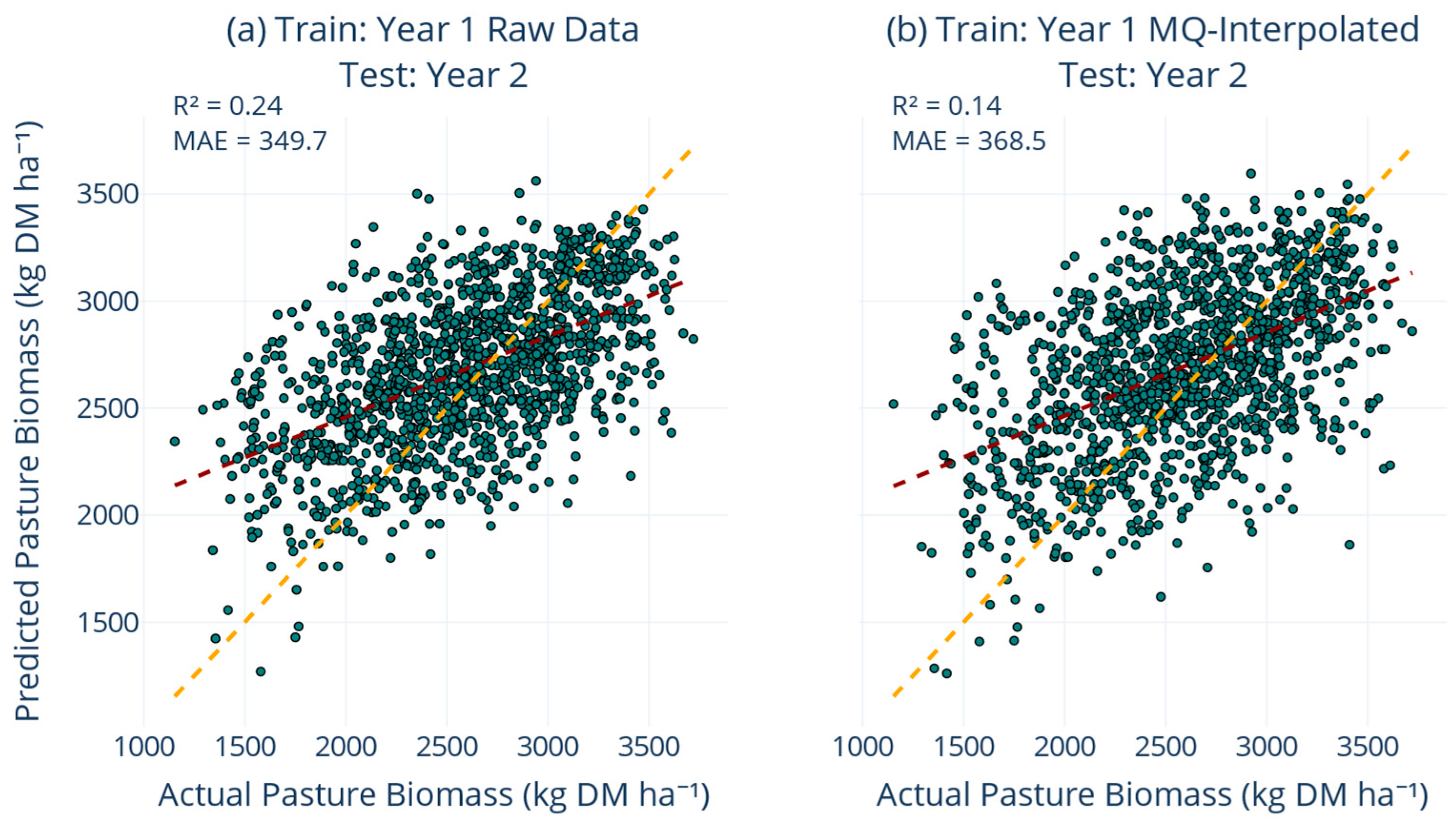
Training exclusively on Year 1 records and projecting onto Year 2 data provides a stringent test of temporal generalisation. When the model was fitted to the raw, non-interpolated Year1Set (1785 rows) and evaluated on the full Year2Set hold-out (1369 rows), it achieved R² = 0.24, MSE = 195,667 kg² DM² ha⁻², RMSE = 442 kg DM ha⁻¹, and MAE = 349 kg DM ha⁻¹ (Figure 8a). However, replacing the raw Year1Set with multiquadric-interpolated values (4242 rows) reduced performance (R² = 0.14, MSE = 220,170 kg² DM² ha⁻², RMSE = 469.22 kg DM ha⁻¹, MAE = 368 kg DM ha⁻¹) as shown in (Figure 8b), while interpolating both years further decreased accuracy (R² = 0.10, MSE = 259,875 kg² DM² ha⁻², RMSE = 510 kg DM ha⁻¹, MAE = 397 kg DM ha⁻¹).

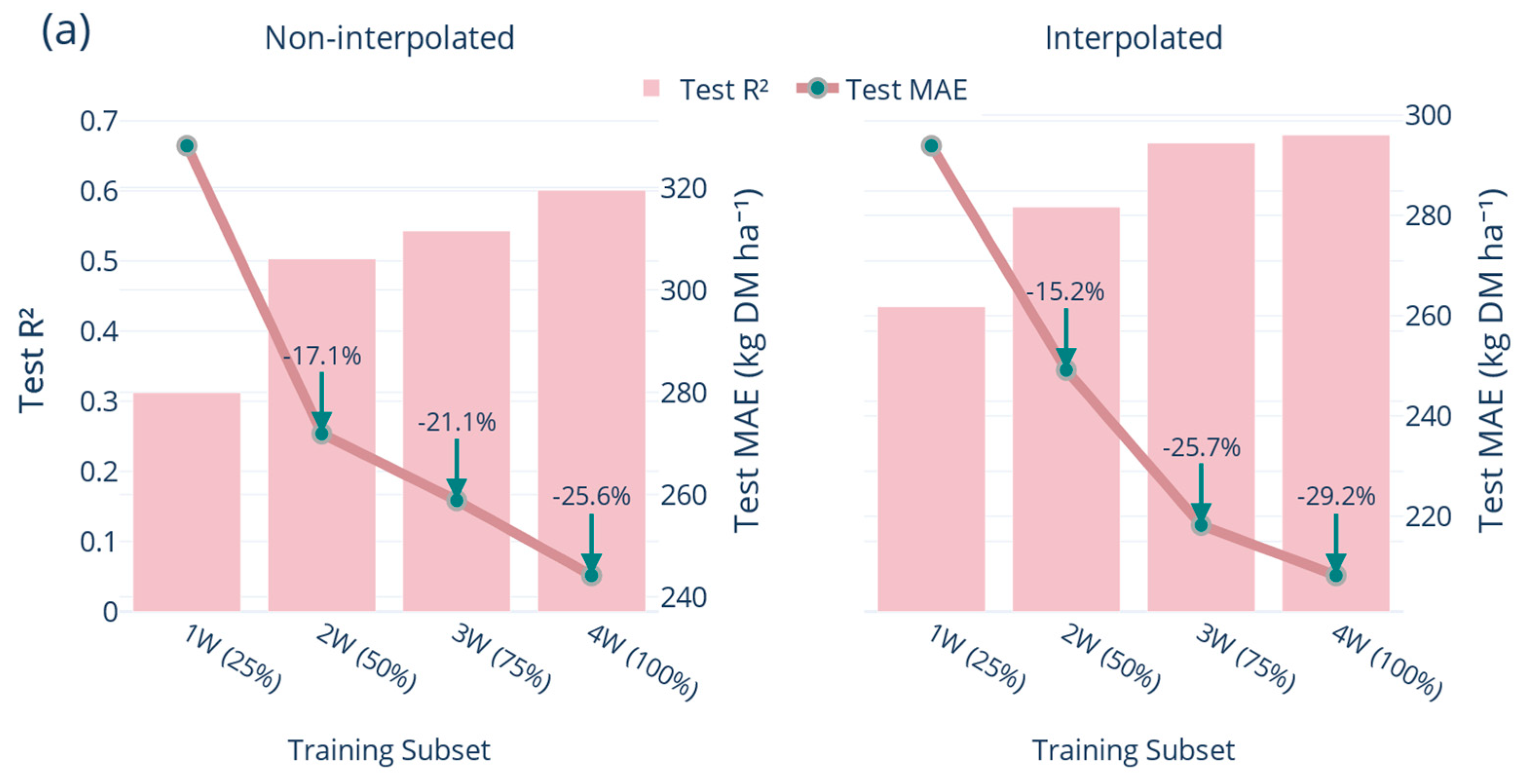
Weekly-observation-mask subsets captured one, two, three, or four weeks of each monthly cycle, corresponding to roughly 25%, 50%, 75%, and 100% of the available chronology. On the non-interpolated data, the test-set R² climbed steadily from 0.31 with the sparsest subset to 0.60 with the full dataset, while MAE fell from 328 to 244 kg DM ha⁻¹ (Figure 9a). Validation on the November 2024 paddocks (n = 41) followed the same trajectory: R² improved from 0.10 to 0.32 and MAE declined from 357 to 307 kg DM ha⁻¹. Accuracy on the sixth-paddock set rose in parallel, reaching R² = 0.30 and MAE = 261 kg DM ha⁻¹ for the complete training span.

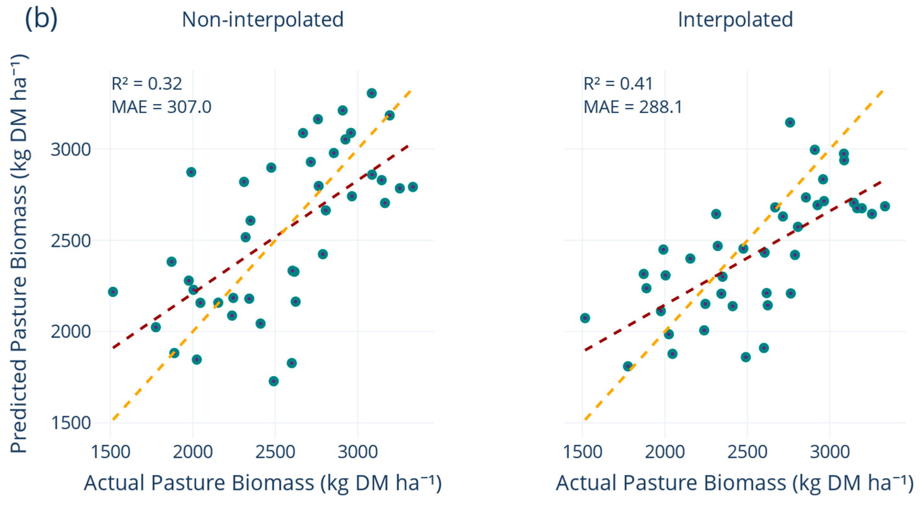
The gains were larger when the progressively expanding archive also contained multiquadric interpolations. With one quarter of the year retained, the interpolated subset already matched the four-week raw model (R² = 0.44, MAE = 294 kg DM ha⁻¹). Assimilating the entire augmented chronology (4486 rows) lifted the test R² to 0.68 and pushed MAE down to 208 kg DM ha⁻¹, a 29% reduction relative to the 1 W baseline (Figure 9b). Crucially, these improvements carried into space and time: on the November 2024 validation R² reached 0.41 with MAE = 288 kg DM ha⁻¹, and on the sixth-paddock set R² climbed to 0.37 with MAE = 255 kg DM ha⁻¹. The scatterplot in Figure 9b shows strong agreement between observed and predicted values with a homogeneous spread of residuals, confirming that the progressive schedule prevents the interpolation surface from over-fitting transient fluctuations. Spatial leave-farm-out experiments provided complementary insight into how well the interpolated model generalises across farms. Holding out one entire farm while training on the remaining 15 farms using the multiquadric-augmented dataset yielded R² = 0.46 and MAE = 299 kg DM ha⁻¹.

A final benchmark evaluated the application of the multiquadric-augmented Sentinel-2 XGBoost model (Section 3.3) by comparing its estimates against Pasture.io; https://pasture.io (PIO), a commercial PB estimation platform. The comparison was conducted on 605 matched observations, where both the developed model and PIO provided estimates for identical paddocks and dates from the 20% test set. The agreement between the two approaches was strong, with an MAE of 240 kg DM ha⁻¹ and the open-source model explaining 66% of the variance in PIO estimates (R² = 0.66). The key findings from this comprehensive analysis have been summarised in

Table 4. Summary of key findings from PB estimation using integrated Sentinel-2 and ML approaches used in this study.

Analysis Component	Key Finding	Performance Metrics
Vegetation Index Limitations	NDVI saturates at ~0.80 when PB exceeds 3000 kg DM ha−1	R2 = 0.19, fan-shaped residual pattern
Optimal Model Configuration	XGBoost with full spectral bands + weather data without indices (non-interpolated)	R2 = 0.63, MAE = 243 kg DM ha−1
Data Augmentation Impact	Multiquadric interpolation (~30% synthetic observations)	Improved to R2 = 0.70, MAE = 216 kg DM ha−1
External Validation	Interpolated model on independent validation sets	Validation Set1: R2 = 0.44, MAE = 267 kg DM ha−1; Validation Set2: R2 = 0.48, MAE = 235 kg DM ha−1
Progressive Training	Continuous updating (1–4 weeks training subsets)	29% MAE reduction from 1 W to 4 W (328 to 208 kg DM ha−1)
Spatial Generalisation	Leave-farm-out validation (trained on 15 farms, tested on 1)	R2 = 0.46, MAE = 299 kg DM ha−1
Commercial Comparison	Benchmarked against Pasture.io platform	R2 = 0.66, MAE = 240 kg DM ha−1
Temporal Limitations	Year1Set to Year2Set extrapolation challenges	Performance declined when training on single year only

below.

4. Discussion

4.1. Exploratory Analysis and Vegetation Index Limitations

Descriptive analysis revealed that PB is governed by seasonality and regional setting, with composite spectral indices explaining daily variation more effectively than instantaneous weather readings. The Pearson correlation heat map (Figure 3) partitioned predictors into three main clusters that informed the modelling strategy. The high auto-correlation among the ten Sentinel-2 bands (r > 0.70) justified the use of tree-based feature selection methods rather than attempting manual dimensional reduction. The greenness-biomass cluster showed that while NDRE (r = 0.49), EVI (0.45), NDVI (0.44) and SAVI (0.44) all correlated positively with PB, none achieved correlation coefficients above 0.50, indicating substantial unexplained variance. The weather cluster revealed tight coupling among maximum temperature, evapotranspiration and solar radiation (r ≈ 0.75) but only weak instantaneous ties to PB (r ≤ 0.18), emphasising the lagged influence of weather on pasture growth rather than same-day effects. These insights guided the development of multi-feature ML pipelines that merged meteorological variables, full-band Sentinel-2 reflectance, red-edge-enhanced indices and categorical predictors to capture the residual variability in PB. The univariate regression analysis (Figure 2) demonstrated that increased sampling does not alleviate the saturation problem inherent in vegetation indices. Saturation occurs when the relationship between a vegetation index and biomass becomes non-linear and eventually plateaus, meaning that increases in biomass no longer result in proportional increases in the index value. The fan-shaped residual pattern confirms that NDVI plateaus near 0.80 while PB continues to rise beyond 3000 kg DM ha⁻¹. Even red-edge information (NDRE), which emerged as the sole significant positive coefficient (+3701 kg DM ha⁻¹ unit⁻¹, p < 0.001), cannot fully capture PB variability once canopies exceed approximately 2800 kg DM ha⁻¹. This saturation fundamentally limits the utility of univariate spectral regressions at high canopy density, where accurate PB estimation is most critical for practical farm management.

An important consideration is that PB variability reflects not only environmental conditions but also management practices, particularly grazing pressure, which can rapidly alter available biomass independent of weather or spectral signals [39,40]. In the absence of explicit management variables, environmental predictors may partly function as categorical site indicators that implicitly capture farm-specific utilisation pattern. This limitation reinforces the necessity of frequent ground-truth calibration through RPM measurements, which inherently integrate both environmental and management effects at each sampling occasion [9,10]. The fortnightly to weekly sampling regime employed here was specifically designed to capture these combined dynamics, while meteorological variables enhanced temporal interpolation between observations [41].

4.2. Overcoming Vegetation Index Saturation Through Multi-Spectral Integration

The primary challenge addressed in this study was the saturation of traditional vegetation indices like NDVI under dense canopies, which typically occurs when PB exceeds approximately 3 tonnes DM ha⁻¹ [42]. This saturation fundamentally limits the utility of conventional remote sensing approaches for practical farm management, where accurate PB estimation is most critical at higher PB levels. The univariate regression analysis (Figure 2) clearly illustrated this limitation, with NDVI plateauing near 0.80 whilst PB continued to rise beyond 3000 kg DM ha⁻¹, resulting in the characteristic fan-shaped residual pattern that confirms the inadequacy of NDVI alone for explaining PB variability.

The integrated approach of combining raw Sentinel-2 reflectance with weather variables demonstrates a clear pathway beyond these limitations. The progression from NDVI-only (R² = 0.28, MAE = 359 kg DM ha⁻¹) to NDVI plus weather factors (R² = 0.50, MAE = 284 kg DM ha⁻¹) to full spectral bands with weather data (R² = 0.63, MAE = 243 kg DM ha⁻¹) clearly shows that whilst weather data provides valuable orthogonal information, the complete Sentinel-2 spectral suite captures essential biophysical information that traditional indices cannot adequately represent. This finding aligns with recent research by Jennewein, et al. [43], who achieved R² = 0.70 for crop biomass/PB estimation using multi-sensor proximal remote sensing combining multiple satellite platforms. However, our current study demonstrates that comparable performance can be achieved using only freely available Sentinel-2 data, highlighting the cost-effectiveness and accessibility of this approach for widespread adoption across diverse farming systems. Collectively these findings demonstrate that PB is governed by a variety of factors such as seasonality and regional setting, that composite spectral indices explain daily variation more effectively than instantaneous weather readings, and that greenness saturation limits the usefulness of univariate spectral regressions at high canopy density.

Guerini Filho, et al. [44] showed that Sentinel-2 imagery combined with vegetation indices could predict natural grassland PB with R² values ranging from 0.51 to 0.65. However, our current study demonstrates that robust predictive performance can be achieved even in the absence of explicit vegetation indices, indicating that raw reflectance bands, especially in the red-edge and short-wave infrared regions, inherently contain the necessary biophysical information. This finding is further supported by Gargiulo, et al. [18], who reported R² = 0.72, RMSE = 255 kg DM/ha⁻¹ when combining Sentinel-2 with Planet CubeSats data, but required multiple commercial satellite sources. The decision to exclude vegetation indices from the final model aligns with findings from Morse-McNabb, et al. [19], who demonstrated that including SWIR bands substantially enhanced yield prediction accuracy with Sentinel-2 when predicting PB above 3000 kg DM ha⁻¹, improving R² from 0.79 to 0.90 and reducing RMSE by nearly 200 kg DM ha⁻¹. Ogungbuyi, et al. [45] similarly highlighted the limitations of index-only approaches, noting that despite a moderate correlation with total PB (R² = 0.43), the associated MAE of 871.83 kg DM ha⁻¹ was too large for practical application. In contrast, the inclusion of SWIR bands, as demonstrated in the current study, not only minimised preprocessing requirements but also improved generalisation on external datasets. The validation results (Figure 5) confirmed that raw red-edge and short-wave-infra-red bands already carry the information encapsulated by the indices, with explicit index calculation adding noise without improving generalisation.

Although weather showed weak instantaneous correlations with PB (Section 3.1), concurrent weather still provides orthogonal information that improves prediction. Removing meteorological inputs lowered test-set R² by 5-6 points and raised MAE by roughly 30 kg DM ha⁻¹, confirming that weather variables capture aspects of pasture condition not reflected in same-day spectral measurements. The ranking of model quality remained unchanged across validation sets, with XGBoost ahead of gradient boosting and random forest, followed by linear methods, showing that ensemble tree algorithms capture non-linear interactions between weather and reflectance that translate beyond the calibration domain. Stand-alone decision trees performed worst, highlighting the stabilising value of ensemble averaging in a feature space dominated by collinear reflectance bands.

Consistent with our findings, Chen, et al. [46] reported optimal PB prediction when all Sentinel-2 bands, NDVI, and weather variables were included, yielding R² approximately 0.60 and MAE approximately 262 kg DM ha⁻¹. This study matched these benchmarks without requiring explicit inclusion of vegetation indices, reinforcing the argument that full spectrum inputs provide a richer predictive foundation than derived indices alone. In a broader modelling context, Netsianda and Mhangara [4] combined Sentinel-2 bands, NDVI, and elevation data to estimate PB using RF and GBM algorithms, achieving an R² of 0.73. Whilst their approach involved multiple data modalities, our findings demonstrate comparable or superior results using only satellite and weather data, without requiring additional topographic inputs.

While this study demonstrated that XGBoost effectively captured information from raw SWIR2 and SWIR3 bands through non-linear feature interactions, future research could explore whether explicit SWIR-based indices such as the Cellulose Absorption Index (CAI) or Normalised Difference Lignin Index (NDLI) provide additional interpretability or improve performance in simpler, more interpretable models (e.g., linear regression or decision trees) that may be preferred in some operational contexts [47]. Recent studies have demonstrated that SWIR bands are particularly effective for predicting high pasture biomass (>4000 kg DM ha⁻¹) where chlorophyll-based indices like NDVI saturate [19,48], and that explicit SWIR-enhanced indices can provide clearer mechanistic insights into canopy structural properties [49,50]. However, our results confirm that ensemble tree-based models can effectively learn these relationships directly from raw spectral bands without requiring pre-calculated indices.

4.3. Data Augmentation Through Multiquadric Interpolation

Cloud cover and satellite revisit cycles create inevitable temporal gaps in optical remote sensing data, a fundamental limitation recognised across the remote sensing literature [4,16]. The multiquadric radial basis interpolation approach employed in this study addresses this limitation by filling gaps in the RPM time series, creating interpolated observations based on actual observations that improve model training without introducing unrealistic temporal assumptions. The interpolation process accounts for pasture growth between measurements by fitting a smooth surface through the observed RPM points, with the multiquadric function providing a mathematically principled way to estimate intermediate values that reflect the gradual accumulation and depletion of biomass between actual field measurements. By confining interpolation strictly to the temporal span defined by observed measurements and requiring at least three actual observations per paddock, the method avoids extrapolation whilst capturing the underlying growth trajectory.

Whilst radial basis interpolation has found application in environmental and medical sciences, and some studies have explored interpolation methods for satellite data in agricultural applications, the specific application of multiquadric interpolation to bridge temporal gaps between ground-truth RPM measurements and cloud-affected satellite imagery in pasture biomass estimation represents a methodological contribution to this field. The observed improvement aligns with recent advances in agricultural data augmentation reported by Gracia Moisés, et al. [51], who demonstrated substantial error reductions using similar techniques in optical spectroscopy applications. However, the application to temporal gap-filling in satellite-ground data integration represents a distinct methodological contribution.

The multiquadric surface employed in this study demonstrated a favourable balance of speed, stability, and predictive effectiveness compared to alternative interpolation methods (Figure 6). This approach contrasted with other interpolation methods such as Gaussian process or Kriging augmentation, which, despite improving spatial homogeneity, are computationally intensive for national-scale datasets [52]. Recent mathematical advancements that generalise the multiquadric kernel for quasi-interpolation [53,54,55] suggest that even higher fidelity could be achieved as these theoretical formulations become operational in geospatial libraries. The trend-assisted multiquadric gridding approach demonstrated efficiency gains noted in Earth observation applications [31], supporting its adoption for operational pasture monitoring systems.

4.4. Progressive Training and Temporal Generalisation

The integration of interpolated rows within the progressive training regime demonstrated the practical benefit of continually updating the model. This trajectory corroborates the findings of Correa-Luna, et al. [10] that even a relatively small proportion of fortnightly ground observations, roughly 10% of paddock days, is sufficient to stabilise pasture predictions whilst emphasising the necessity of retraining the model on a comparable rolling schedule.

However, the temporal validation experiments (Figure 8) revealed important limitations of interpolation when applied to strict temporal extrapolation scenarios. Training exclusively on Year1Set and testing on Year2Set demonstrated that interpolation actually reduced performance compared to the raw data baseline (R² slipped from 0.24 to 0.14, MAE rose from 349 to 368 kg DM ha⁻¹). This apparent contradiction with the overall benefits of interpolation highlights the context-dependent nature of data augmentation techniques. This finding aligns with domain adaptation challenges widely reported in ML literature Meyer, et al. [56]. To understand this performance decline, we decomposed the prediction error into bias and variance components. The interpolated Year1Set model exhibited higher bias (systematic underestimation of Year2 biomass by approximately 15%) and similar variance compared to the raw model, suggesting that the interpolation surface captured Year1-specific patterns that did not transfer to Year2 conditions.

The observations generated through interpolation introduced bias when the training and testing data came from fundamentally different temporal distributions, as the interpolation surface fitted to Year 1 data encoded seasonal patterns specific to that year. However, when training and testing data came from similar temporal distributions (the 80:20 split from the combined dataset), interpolation significantly improved performance by providing a denser, more representative sample of the underlying growth patterns. In summary, these findings also indicate that the combined application of interpolation and progressive training effectively bridges inherent observational gaps associated with optical remote sensing and establishes a data-efficient method for maintaining accuracy as seasonal conditions change. The comprehensive strategy directly addresses model validity and reliability across varied climatic, soil, and management contexts, thereby offering a robust and generalisable solution.

4.5. Model Performance and Validation Across Multiple Scales

The robustness of the final multiquadric-augmented model was reflected across external validation sets (Figure 7). The model achieved consistent performance on the November 2024 paddocks and the sixth-paddock validation sets, outperforming the non-interpolated baseline whilst other interpolation methods failed to surpass an R² of 0.37. Spatial leave-farm-out experiments confirmed that a PB model trained on one set of paddocks inevitably experiences a reduction in accuracy when applied to entirely excluded fields. In our case, the non-interpolated version surrendered roughly one quarter of its explanatory power under this scenario, a decline consistent with cross-location deterioration reported by Smith, et al. [57]. However, the introduction of multiquadric interpolation significantly mitigated this loss, helping the model maintain a more balanced representation of the growth envelope and maintaining the MAE on the held-out farms below 300 kg DM ha⁻¹, while explaining nearly half of the PB variance, surpassing the more complex ensembles assessed by Smith, et al. [57] at comparable extrapolation distances.

The disparity between robust performance on the internal 20% test split and comparatively weaker scores on independent validation sets elucidates the inherent challenges associated with model transferability, as widely reported in remote sensing applications where models are tested beyond their calibration domain. Validation errors exceeded test errors by about 10%, reflecting the additional temporal and geographic distance embodied in the hold-out samples. Nevertheless, the crucial need for regular retraining is emphasised by the observation that model accuracy declined on paddocks and seasons withheld from calibration, even with interpolation. Overall, the results demonstrate that temporal generalisation hinges on two complementary strategies, retaining the full historical record so that the model learns from experiencing the complete seasonal duration, and supplementing that record with cautiously smoothed interpolations that densify the signal without inflating noise. When applied together, these measures raise R2 by about 30% points and cut MAE by roughly 85 kg DM ha⁻¹ compared with a model trained on a single season and maintain consistent accuracy when entire farms are withheld during testing. The consistency of these results across scenarios shows that the model, built with the full predictor set, extends reliably to farms unseen during calibration, reinforcing the temporal gains reported above.

4.6. Comparison with Commercial Decision-Support Systems

The comparison with PIO, a commercial PB estimation platform, provides crucial context for the application of research-based approaches. The strong agreement between the developed open-source model and the proprietary platform (R² = 0.66, MAE = 240 kg DM ha⁻¹) demonstrates that transparent, academic approaches can achieve comparable performance to commercial solutions across matched observations spanning multiple farms and production years [10]. This benchmark was performed across multiple farms and distinct production years, demonstrating that an openly documented and fully reproducible approach can achieve relatively high performance whilst retaining adaptability to integrate new sensors and management variables as they become available. Commercial platforms typically have access to multiple satellite sources, sophisticated atmospheric correction algorithms, and proprietary data fusion techniques, making this performance parity particularly significant. The comparison validates methodological choices whilst highlighting the potential for democratising precision agriculture technologies. Many existing commercial solutions require significant capital investment or ongoing subscription costs that may be prohibitive for smaller farming operations, particularly in developing regions where cost-effective monitoring solutions are most needed.

4.7. Limitations and Future Research Directions

Several factors constrain the current implementation and highlight avenues for future research. The reliance on multiquadric interpolation presumes gradual temporal evolution of PB, a common approach for filling cloudy gaps in vegetation monitoring but one that risks obscuring sharp declines associated with grazing or drought. Combining optical-derived indices with sensors capable of detecting rapid canopy structural shifts, such as C-band radar backscatter, could offset this limitation [58]. Pasture greenness measures displayed the well-recognised saturation effect once biomass exceeded roughly 3000 kg DM ha⁻¹, thereby limiting model sensitivity in the critical range where tactical management adjustments are most often needed [46,59]. Acquiring richer spectral information, such as narrow-band hyperspectral or chlorophyll fluorescence signals, may offer enhanced sensitivity under high biomass and address this ceiling effect [13,60,61].

Additionally, weather predictors were restricted to daily aggregates, limiting capacity to reflect sub-daily factors such as vapour pressure deficit, refined soil moisture estimates, or high-resolution temperature extremes that could potentially capture short-lived stress events influencing pasture growth between satellite overpasses. The study spanned three districts within a single coastal climatic zone, and explicit testing of site-specific differences in management such as fertiliser timing or detailed pasture quality was not conducted. As noted by Holzworth, et al. [62], expansion of ground data across diverse weather and management systems is essential to evaluate broad-scale model transferability. The Year 1 to Year 2 transfer experiment reinforces this point because despite a threefold increase in sample size through interpolation, a model trained exclusively on the first season could not accommodate phenological shifts of the following year, with acceptable performance only restored after expanding the calibration base and retraining on multi-year data [63].

The demonstrated performance achievements using freely available satellite data have important implications for democratising precision agriculture technologies. The open-source approach provides full methodological transparency allowing for local adaptation and improvement, eliminates ongoing data acquisition costs through use of freely available Sentinel-2 data, and enables integration of additional sensor types or management variables as they become available. However, the current implementation may require some technical expertise, making it more immediately accessible to researchers, government agents, or technical staff rather than directly to individual farmers. Strategically, the progressive training paradigm establishes a pathway for continuously improving models that remain reliable as satellite technology, weather conditions, and management practices evolve.

Methodologically, this study significantly advances pasture remote sensing by demonstrating that integrating raw spectral, meteorological, and management data within a unified machine learning framework provides superior performance compared to models driven solely by vegetation indices. From a practical standpoint, the interpolation-enhanced model delivers near real-time PB estimates that align well with commercial platforms across diverse environments, offering producers a transparent and customisable alternative to proprietary solutions. Future work should focus on exploring ensemble combinations of optical and radar imagery, automating paddock-level recalibration using farmer-supplied RPM pasture biomass measurements, and integrating the model into grazing allocation tools to directly translate predictive accuracy into measurable productivity gains and farm profitability. These enhancements will enable integration into grazing allocation tools, establishing a dynamic, self-improving decision-support system that translates predictive accuracy into improved pasture utilisation and increased farm profitability.

5. Conclusions

This study demonstrates that accurate pasture biomass estimation can be achieved even where traditional vegetation indices saturate and Sentinel-2 imagery is intermittently obscured by cloud cover. By integrating raw multispectral reflectance, rising plate-meter measurements, daily weather data, and paddock-level metadata within a machine learning framework, the model effectively bridged the gap between satellite observations and ground measurements. The unified strategy prioritising full-band reflectance over vegetation indices achieved robust baseline performance (R² = 0.63, MAE = 243 kg DM ha⁻¹), substantially outperforming NDVI-based approaches. Multiquadric radial basis interpolation of field measurements addressed temporal gaps from cloud obstruction, augmenting the dataset with approximately 30% interpolated observations and improving performance to R² = 0.70 and MAE = 216 kg DM ha⁻¹. These improvements were observed across independent validation sets, with the November 2024 validation set achieving R² = 0.44 and MAE = 267 kg DM ha⁻¹, and the sixth-paddock validation set achieving R² = 0.48 and MAE = 235 kg DM ha⁻¹.

The implementation of progressive training with seasonally aligned observations-maintained model accuracy across temporal and spatial contexts. Leave-farm-out validation confirmed robust generalisation to unseen farms (R² = 0.46, MAE < 300 kg DM ha⁻¹), whilst comparison with the commercial Pasture.io platform demonstrated comparable performance using freely available data. Despite these advancements, several limitations warrant future research, as multiquadric interpolation may smooth abrupt pasture biomass declines following intensive grazing, and daily weather aggregates may overlook short-lived environmental events. Future work should focus on integrating finer-resolution sensors, developing automated paddock-level recalibration systems, and incorporating the model into grazing allocation tools to establish a dynamic decision-support system that translates predictive accuracy into improved pasture utilisation and farm profitability.

References

1. Ali, I.; Cawkwell, F.; Dwyer, E.; Green, S. Modeling Managed Grassland Biomass Estimation by Using Multitemporal Remote Sensing Data—A Machine Learning Approach. IEEE J. Sel. Top. Appl. Earth Obs. Remote Sens. 2017, 10, 3254–3264. [Google Scholar] [CrossRef]
2. Shi, Y.; Gao, J.; Li, X.; Li, J.; Torre, D.M.G.D.; Brierley, G.J. Improved Estimation of Aboveground Biomass of Disturbed Grassland through Including Bare Ground and Grazing Intensity. Remote Sens. 2021, 13, 2105. [Google Scholar] [CrossRef]
3. Pang, H.; Zhang, A.; Kang, X.; He, N.; Dong, G. Estimation of the Grassland Aboveground Biomass of the Inner Mongolia Plateau Using the Simulated Spectra of Sentinel-2 Images. Remote Sens. 2020, 12, 4155. [Google Scholar] [CrossRef]
4. Netsianda, A.; Mhangara, P. Aboveground biomass estimation in a grassland ecosystem using Sentinel-2 satellite imagery and machine learning algorithms. Environ. Monit. Assess. 2025, 197, 138. [Google Scholar] [CrossRef] [PubMed]
5. Wang, Z.; Ma, Y.; Zhang, Y.; Shang, J. Review of Remote Sensing Applications in Grassland Monitoring. Remote Sens. 2022, 14, 2903. [Google Scholar] [CrossRef]
6. Radočaj, D.; Šiljeg, A.; Marinović, R.; Jurišić, M. State of Major Vegetation Indices in Precision Agriculture Studies Indexed in Web of Science: A Review. Agriculture 2023, 13, 707. [Google Scholar] [CrossRef]
7. de Alckmin, G.T.; Kooistra, L.; Rawnsley, R.; Lucieer, A. Comparing methods to estimate perennial ryegrass biomass: Canopy height and spectral vegetation indices. Precis. Agric. 2021, 22, 205–225. [Google Scholar] [CrossRef]
8. Vidican, R.; Mălinaș, A.; Ranta, O.; Moldovan, C.; Marian, O.; Ghețe, A.; Ghișe, C.R.; Popovici, F.; Cătunescu, G.M. Using Remote Sensing Vegetation Indices for the Discrimination and Monitoring of Agricultural Crops: A Critical Review. Agronomy 2023, 13, 3040. [Google Scholar] [CrossRef]
9. Gargiulo, J.I.; Lyons, N.A.; Masia, F.; Beale, P.; Insua, J.R.; Correa-Luna, M.; Garcia, S.C. Comparison of Ground-Based, Unmanned Aerial Vehicles and Satellite Remote Sensing Technologies for Monitoring Pasture Biomass on Dairy Farms. Remote Sens. 2023, 15, 2752. [Google Scholar] [CrossRef]
10. Correa-Luna, M.; Gargiulo, J.; Beale, P.; Deane, D.; Leonard, J.; Hack, J.; Geldof, Z.; Wilson, C.; Garcia, S. Accounting for minimum data required to train a machine learning model to accurately monitor Australian dairy pastures using remote sensing. Sci. Rep. 2024, 14, 16927. [Google Scholar] [CrossRef]
11. Askari, M.S.; McCarthy, T.; Magee, A.; Murphy, D.J. Evaluation of Grass Quality under Different Soil Management Scenarios Using Remote Sensing Techniques. Remote Sens. 2019, 11, 1835. [Google Scholar] [CrossRef]
12. De Rosa, D.; Basso, B.; Fasiolo, M.; Friedl, J.; Fulkerson, B.; Grace, P.R.; Rowlings, D.W. Predicting pasture biomass using a statistical model and machine learning algorithm implemented with remotely sensed imagery. Comput. Electron. Agric. 2021, 180, 105880. [Google Scholar] [CrossRef]
13. Zhang, H.; Sun, Y.; Chang, L.; Qin, Y.; Chen, J.; Qin, Y.; Du, J.; Yi, S.; Wang, Y. Estimation of Grassland Canopy Height and Aboveground Biomass at the Quadrat Scale Using Unmanned Aerial Vehicle. Remote Sens. 2018, 10, 851. [Google Scholar] [CrossRef]
14. Naidoo, L.; van Deventer, H.; Ramoelo, A.; Mathieu, R.; Nondlazi, B.; Gangat, R. Estimating above ground biomass as an indicator of carbon storage in vegetated wetlands of the grassland biome of South Africa. Int. J. Appl. Earth Obs. Geoinf. 2019, 78, 118–129. [Google Scholar] [CrossRef]
15. Nguyen, H.T.T.; Doan, T.M.; Tomppo, E.; McRoberts, R.E. Land Use/Land Cover Mapping Using Multitemporal Sentinel-2 Imagery and Four Classification Methods—A Case Study from Dak Nong, Vietnam. Remote Sens. 2020, 12, 1367. [Google Scholar] [CrossRef]
16. Dubovik, O.; Schuster, G.L.; Xu, F.; Hu, Y.; Bösch, H.; Landgraf, J.; Li, Z. Grand Challenges in Satellite Remote Sensing. Front. Remote Sens. 2021, 2, 619818. [Google Scholar] [CrossRef]
17. César, I.A.-M.; Guzman, D.; Casas, J.; Bastidas, M.; Polanco, J.; Valencia-Ortiz, M.; Montenegro, F.; Arango, J.; Ishitani, M.; Selvaraj, M.G. Predictive Modeling of Above-Ground Biomass in Brachiaria Pastures from Satellite and UAV Imagery Using Machine Learning Approaches. Remote Sens. 2022, 14, 5870. [Google Scholar] [CrossRef]
18. Gargiulo, J.; Clark, C.; Lyons, N.; de Veyrac, G.; Beale, P.; Garcia, S. Spatial and Temporal Pasture Biomass Estimation Integrating Electronic Plate Meter, Planet CubeSats and Sentinel-2 Satellite Data. Remote Sens. 2020, 12, 3222. [Google Scholar] [CrossRef]
19. Morse-McNabb, E.M.; Hasan, M.F.; Karunaratne, S. A Multi-Variable Sentinel-2 Random Forest Machine Learning Model Approach to Predicting Perennial Ryegrass Biomass in Commercial Dairy Farms in Southeast Australia. Remote Sens. 2023, 15, 2915. [Google Scholar] [CrossRef]
20. Amarsaikhan, E.; Erdenebaatar, N.; Amarsaikhan, D.; Otgonbayar, M.; Bayaraa, B. Estimation and mapping of pasture biomass in Mongolia using machine learning methods. Geocarto Int. 2023, 38, 2195824. [Google Scholar] [CrossRef]
21. Banerjee, P. MODIS-FIRMS and ground-truthing-based wildfire likelihood mapping of Sikkim Himalaya using machine learning algorithms. Nat. Hazards 2022, 110, 899–935. [Google Scholar] [CrossRef]
22. Vahidi, M.; Shafian, S.; Thomas, S.; Maguire, R. Pasture Biomass Estimation Using Ultra-High-Resolution RGB UAVs Images and Deep Learning. Remote Sens. 2023, 15, 5714. [Google Scholar] [CrossRef]
23. Johnson, I.R.; Chapman, D.F.; Snow, V.O.; Eckard, R.J.; Parsons, A.J.; Lambert, M.G.; Cullen, B.R. DairyMod and EcoMod: Biophysical pasture-simulation models for Australia and New Zealand. Aust. J. Exp. Agric. 2008, 48, 621–631. [Google Scholar] [CrossRef]
24. Vaze, J.; Johnston, W.H.; Teng, J.; Tuteja, N.K.; Johnson, I. Development and implementation of a generic pasture growth model (CLASS PGM). Environ. Model. Softw. 2009, 24, 107–114. [Google Scholar] [CrossRef]
25. Johnson, I.R.; Lodge, G.M.; White, R.E. The Sustainable Grazing Systems Pasture Model: Description, philosophy and application to the SGS National Experiment. Aust. J. Exp. Agric. 2003, 43, 711–728. [Google Scholar] [CrossRef]
26. Moore, A.D.; Holzworth, D.P.; Herrmann, N.I.; Huth, N.I.; Robertson, M.J. The Common Modelling Protocol: A hierarchical framework for simulation of agricultural and environmental systems. Agric. Syst. 2007, 95, 37–48. [Google Scholar] [CrossRef]
27. Keating, B.A. APSIM’s origins and the forces shaping its first 30 years of evolution: A review and reflections. Agron. Sustain. Dev. 2024, 44, 24. [Google Scholar] [CrossRef]
28. Jones, J.W.; Antle, J.M.; Basso, B.; Boote, K.J.; Conant, R.T.; Foster, I.; Godfray, H.C.J.; Herrero, M.; Howitt, R.E.; Janssen, S.; et al. Toward a new generation of agricultural system data, models, and knowledge products: State of agricultural systems science. Agric. Syst. 2017, 155, 269–288. [Google Scholar] [CrossRef] [PubMed]
29. Huang, J.; Tian, L.; Liang, S.; Ma, H.; Becker-Reshef, I.; Huang, Y.; Su, W.; Zhang, X.; Zhu, D.; Wu, W. Assimilating a synthetic Kalman filter leaf area index series into the WOFOST model to improve regional winter wheat yield estimation. Agric. For. Meteorol. 2016, 216, 188–202. [Google Scholar] [CrossRef]
30. Ogungbuyi, M.G.; Guerschman, J.; Fischer, A.M.; Crabbe, R.A.; Ara, I.; Mohammed, C.; Scarth, P.; Tickle, P.; Whitehead, J.; Harrison, M.T. Improvement of pasture biomass modelling using high-resolution satellite imagery and machine learning. J. Environ. Manag. 2024, 356, 120564. [Google Scholar] [CrossRef]
31. Liu, H.; Guo, P.; Liu, J.; Liu, R.; Tong, T. An Extension of Multiquadric Method Based on Trend Analysis for Surface Construction. IEEE J. Sel. Top. Appl. Earth Obs. Remote Sens. 2023, 16, 3435–3441. [Google Scholar] [CrossRef]
32. Zhu, Z.; Woodcock, C.E. Object-based cloud and cloud shadow detection in Landsat imagery. Remote Sens. Environ. 2012, 118, 83–94. [Google Scholar] [CrossRef]
33. Nuss, W.A.; Titley, D.W. Use of Multiquadric Interpolation for Meteorological Objective Analysis. Mon. Weather Rev. 1994, 122, 1611–1631. [Google Scholar] [CrossRef]
34. Powell, M. Radial Basis Function Methods for Interpolation to Functions of Many Variables. HERMIS Int. J. Comput. Maths Appl. 2002, 3. [Google Scholar]
35. Anjyo, K.; Lewis, J.P. RBF Interpolation and Gaussian Process Regression Through an RKHS Formulation. J. Math. Ind. 2011, 3, 63–71. [Google Scholar]
36. Mishra, P.K.; Nath, S.K.; Sen, M.K.; Fasshauer, G.E. Hybrid Gaussian-cubic radial basis functions for scattered data interpolation. Comput. Geosci. 2018, 22, 1203–1218. [Google Scholar] [CrossRef]
37. Jasek, K.; Pasternak, M.; Miluski, W.; Bugaj, J.; Grabka, M. Application of Gaussian Radial Basis Functions for Fast Spatial Imaging of Ground Penetration Radar Data Obtained on an Irregular Grid. Electronics 2021, 10, 2965. [Google Scholar] [CrossRef]
38. Smith, W.H.F.; Wessel, P. Gridding with continuous curvature splines in tension. Geophysics 1990, 55, 293–305. [Google Scholar] [CrossRef]
39. Török, P.; Lindborg, R.; Eldridge, D.; Pakeman, R. Grazing effects on vegetation: Biodiversity, management, and restoration. Appl. Veg. Sci. 2024, 27, e12794. [Google Scholar] [CrossRef]
40. Hassan, N.; Wang, Z. Paralleled grazing and mowing differentially affected plant community diversity and productivity in a semi-arid grassland. Ecol. Process. 2024, 13, 62. [Google Scholar] [CrossRef]
41. Cândido, B.; Mindala, U.; Ebrahimy, H.; Zhang, Z.; Kallenbach, R. Integrating Proximal and Remote Sensing with Machine Learning for Pasture Biomass Estimation. Sensors 2025, 25, 1987. [Google Scholar] [CrossRef]
42. Mutanga, O.; Masenyama, A.; Sibanda, M. Spectral saturation in the remote sensing of high-density vegetation traits: A systematic review of progress, challenges, and prospects. ISPRS J. Photogramm. Remote Sens. 2023, 198, 297–309. [Google Scholar] [CrossRef]
43. Jennewein, J.S.; Davis, B.W.; Seehaver-Eagen, S.; Nicolette, J.; Pittman, J.; Hively, W.D.; Goldsmith, A.; Hidalgo, C.; Reberg-Horton, C.; Mirsky, S.B. Multi-sensor proximal remote sensing for cover crop biomass estimation at high and moderate spatial resolutions. Smart Agric. Technol. 2025, 12, 101201. [Google Scholar] [CrossRef]
44. Filho, M.G.; Kuplich, T.M.; Quadros, F.L.F.D. Estimating natural grassland biomass by vegetation indices using Sentinel 2 remote sensing data. Int. J. Remote Sens. 2020, 41, 2861–2876. [Google Scholar] [CrossRef]
45. Ogungbuyi, M.G.; Guerschman, J.; Fischer, A.M.; Mohammed, C.; Crabbe, R.A.; Harrison, M.T. Using vegetation indices from nanosatellites for timely prediction of pasture biomass. Total Environ. Adv. 2025, 15, 200130. [Google Scholar] [CrossRef]
46. Chen, Y.; Guerschman, J.; Shendryk, Y.; Henry, D.; Harrison, M.T. Estimating Pasture Biomass Using Sentinel-2 Imagery and Machine Learning. Remote Sens. 2021, 13, 603. [Google Scholar] [CrossRef]
47. Nagler, P.L.; Inoue, Y.; Glenn, E.P.; Russ, A.L.; Daughtry, C.S.T. Cellulose absorption index (CAI) to quantify mixed soil–plant litter scenes. Remote Sens. Environ. 2003, 87, 310–325. [Google Scholar] [CrossRef]
48. Cai, T.; Chang, C.; Zhao, Y.; Wang, X.; Yang, J.; Dou, P.; Otgonbayar, M.; Zhang, G.; Zeng, Y.; Wang, J. Within-season estimates of 10 m aboveground biomass based on Landsat, Sentinel-2 and PlanetScope data. Sci. Data 2024, 11, 1276. [Google Scholar] [CrossRef] [PubMed]
49. Tian, Z.; Fan, J.; Yu, T.; Leon, N.; Kaeppler, S.; Zhang, Z. Mitigating NDVI saturation in imagery of dense and healthy vegetation. ISPRS J. Photogramm. Remote Sens. 2025, 227, 234–250. [Google Scholar] [CrossRef]
50. Ranjbar, S.; Losos, D.; Dechant, B.; Hoffman, S.; Başakın, E.E.; Stoy, P.C. Harnessing Information From Shortwave Infrared Reflectance Bands to Enhance Satellite-Based Estimates of Gross Primary Productivity. J. Geophys. Res. Biogeosci. 2024, 129, e2024JG008240. [Google Scholar] [CrossRef]
51. Moisés, A.G.; Pascual, I.V.; González, J.J.I.; Zamarreño, C.R. Data Augmentation Techniques for Machine Learning Applied to Optical Spectroscopy Datasets in Agrifood Applications: A Comprehensive Review. Sensors 2023, 23, 8562. [Google Scholar] [CrossRef]
52. Ferber, F.F.; Gay, D.; Soulié, J.-C.; Diatta, J.; Maillard, O.-A. Kriging and Gaussian Process Interpolation for Georeferenced Data Augmentation. arXiv 2025, arXiv:2501.07183. [Google Scholar] [CrossRef]
53. Kumar, A.; Sharma, A.; Singh, A.K.; Singh, S.K.; Saxena, S. Data Augmentation for Medical Image Classification Based on Gaussian Laplacian Pyramid Blending With a Similarity Measure. IEEE J. Biomed. Health Inform. 2023, 29, 3886–3893. [Google Scholar] [CrossRef] [PubMed]
54. Ortmann, M.; Buhmann, M. High accuracy quasi-interpolation using a new class of generalized multiquadrics. J. Math. Anal. Appl. 2024, 538, 128359. [Google Scholar] [CrossRef]
55. Sommariva, A.; Vianello, M. Random sampling and polynomial-free interpolation by Generalized MultiQuadrics. J. Approx. Theory 2025, 306, 106119. [Google Scholar] [CrossRef]
56. Meyer, H.; Reudenbach, C.; Hengl, T.; Katurji, M.; Nauss, T. Improving performance of spatio-temporal machine learning models using forward feature selection and target-oriented validation. Environ. Model. Softw. 2018, 101, 1–9. [Google Scholar] [CrossRef]
57. Smith, H.D.; Dubeux, J.C.B.; Zare, A.; Wilson, C.H. Assessing Transferability of Remote Sensing Pasture Estimates Using Multiple Machine Learning Algorithms and Evaluation Structures. Remote Sens. 2023, 15, 2940. [Google Scholar] [CrossRef]
58. Veloso, A.; Mermoz, S.; Bouvet, A.; Le Toan, T.; Planells, M.; Dejoux, J.-F.; Ceschia, E. Understanding the temporal behavior of crops using Sentinel-1 and Sentinel-2-like data for agricultural applications. Remote Sens. Environ. 2017, 199, 415–426. [Google Scholar] [CrossRef]
59. Mutanga, O.; Skidmore, A. Hyperspectral band depth analysis for a better estimation of grass biomass (Cenchrus ciliaris) measured under controlled laboratory conditions. Int. J. Appl. Earth Obs. Geoinf. 2004, 5, 87–96. [Google Scholar] [CrossRef]
60. Mohammed, G.H.; Colombo, R.; Middleton, E.M.; Rascher, U.; van der Tol, C.; Nedbal, L.; Goulas, Y.; Pérez-Priego, O.; Damm, A.; Meroni, M.; et al. Remote sensing of solar-induced chlorophyll fluorescence (SIF) in vegetation: 50 years of progress. Remote Sens. Environ. 2019, 231, 111177. [Google Scholar] [CrossRef]
61. Zhang, Y.; Migliavacca, M.; Penuelas, J.; Ju, W. Advances in hyperspectral remote sensing of vegetation traits and functions. Remote Sens. Environ. 2021, 252, 112121. [Google Scholar] [CrossRef]
62. Holzworth, D.; Huth, N.I.; Devoil, P.G.; Zurcher, E.J.; Herrmann, N.I.; McLean, G.; Chenu, K.; van Oosterom, E.J.; Snow, V.; Murphy, C.; et al. APSIM—Evolution towards a new generation of agricultural systems simulation. Environ. Model. Softw. 2014, 62, 327–350. [Google Scholar] [CrossRef]
63. Kyere, I.; Astor, T.; Graß, R.; Wachendorf, M. Multi-Temporal Agricultural Land-Cover Mapping Using Single-Year and Multi-Year Models Based on Landsat Imagery and IACS Data. Agronomy 2019, 9, 309. [Google Scholar] [CrossRef]
Figure 1. Geographic distribution of study farms across coastal districts of New South Wales, Australia used in the study. This illustrates the spatial distribution of the 16 commercial dairy farms included in this study, located across three coastal districts of New South Wales (NSW), Australia. Farms were grouped into the mid-coast (n = 7), south coast (n = 5), and north coast (n = 4) regions, as defined in Section 2.1. Marker positions represent jittered farm centroids derived from paddock-level coordinates, with a small random displacement applied to protect commercial confidentiality. Regional shading represents the general geographic coverage of each study district. An inset map of Australia highlights the location of NSW relative to the broader states.
Remotesensing 17 03787 g001
Figure 2. Combined regression and validation of pasture biomass (PB) estimates. Panel (a) shows the linear regression (LR) between Normalised Difference Vegetation Index (NDVI) and rising plate-meter biomass (kg DM ha−1) measurements, with a teal regression line, a shaded 95% prediction interval, and the fitted equation plus R2 annotation. Panels (bd) depict actual versus predicted PB for 80:20, 70:30 and 60:40 train–test splits using LR, respectively; each includes a teal regression line, an orange dashed 1:1 line, the 95% confidence band around the predicted values, and the corresponding R2.
Remotesensing 17 03787 g002
Figure 3. Pearson-correlation heatmap of selected biophysical, spectral, and meteorological variables. Pasture biomass (PB, kg DM ha−1); weather variables include daily maximum temperature (T.Max, °C), daily minimum temperature (T.Min, °C), evapotranspiration (Evap, mm), incoming solar radiation (Radn, MJ m−2), vapour pressure (VP, kPa), precipitation (Rainfall, mm), maximum relative humidity (RHmaxT, %), and minimum relative humidity (RHminT, %); spectral bands comprise Blue (blue band), Green (green band), Red (red band), NIR (near-infrared band), RedEdge1, RedEdge2, and RedEdge3 (red edge bands 1−3), and SWIR2 and SWIR3 (short-wave infrared bands 2−3); vegetation indices include NDVI (Normalised Difference Vegetation Index), SAVI (Soil Adjusted Vegetation Index), EVI (Enhanced Vegetation Index), and NDRE (Normalised Difference Red Edge Index).
Remotesensing 17 03787 g003
Figure 4. Scatterplots of actual versus predicted PB (kg DM ha−1) on the non-interpolated test set (n = 633 rows) for four predictor scenarios. Panels (ad) correspond, respectively, to (a) all spectral bands plus vegetation indices (NDVI, SAVI, EVI, NDRE) without weather data; (b) all spectral bands with weather variables and vegetation indices; (c) spectral bands alone without indices or weather data; and (d) spectral bands with weather variables but without indices. Each panel displays its R2, RMSE, and MAE (kg DM ha−1) in the top left corner. The maroon dashed line represents the fitted regression line, and the orange dashed line shows the one-to-one line.
Remotesensing 17 03787 g004
Figure 5. Scatterplots of actual versus predicted PB (kg DM ha−1) on two independent validation sets for the non-interpolated scenario. All the bands with weather data without vegetation indices (NDVI, SAVI, EVI, NDRE). Panel (a) shows the November 2024 paddocks (the main five monitored paddocks per farm; n = 41 rows), and panel (b) shows the sixth extra paddock monitored for each farm (n = 63 rows) with axes starting at a minimum of 1500 kg DM ha−1. Both subplots are based solely on spectral bands (no vegetation indices) and include their R2, RMSE, and MAE (kg DM ha−1) in the top-left corner. The maroon dashed line represents the regression line, and the orange dashed line indicates the one-to-one line.
Remotesensing 17 03787 g005
Figure 6. Impact of different interpolation methods on XGBoost model performance using the “All the Bands with Weather Data without Indices” feature set. In every panel, test R2 is shown as pink bars and test MAE by a light-pink line with teal markers; at each MAE point, the teal arrow indicates the percentage increase (upward) or decrease (downward) relative to the non-interpolated (Non_ip) baseline. Panel (a) (top left) shows Year1Set (pre −April 2023) interpolation methods, polynomial (poly2), RBF, multiquadric (mq), and minimum-curvature (mcg). Panel (b) (top right) shows the same four methods applied in Year2Set (post −1 April 2023). Panel (c) (centre bottom) illustrates the performance of these four interpolation methods when applied to the full two-year period.
Remotesensing 17 03787 g006
Figure 7. Observed versus predicted PB (kg DM ha−1) obtained with the XGBoost model trained on the multiquadric interpolated data. Panels: (a) test set; (b) validation set—November 2024 (main five monitored paddocks per farm; n = 41); (c) validation set—sixth extra paddock per farm (n = 63). The maroon dashed line represents the regression fit, and the orange dashed line denotes the 1:1 relationship between actual and predicted PB estimates.
Remotesensing 17 03787 g007
Figure 8. Comparison of observed versus predicted PB (kg DM ha−1) when training on Year 1 data and testing on Year 2 data. Panel (a) shows the model trained on raw (non-interpolated) Year 1 data → Year 2 Test, while panel (b) shows the model trained on Year 1 multiquadric-interpolated data → Year 2 Test. Each panel plots actual versus predicted values for the Year 2 hold-out, with annotated R2 and MAE. The maroon dashed line represents the regression fit, and the orange dashed line denotes the 1:1 relationship between actual and predicted PB estimates.
Remotesensing 17 03787 g008
Figure 9. Progressive-training performance of the XGBoost PB model built from the “All the Bands with Weather Data without Indices” feature set. (a) Pink bars show the test-set R2 for each weekly-observation-mask (WOM) subset: 1 W (25%), 2 W (50%), 3 W (75%), and 4 W (100%). The light-pink line with teal markers depicts the corresponding test MAE; teal arrows indicate the percentage change in MAE relative to the 1 W (25%) baseline (upward for increases, downward for decreases). (b) Observed versus predicted PB (kg DM ha−1) on the validation set—November 2024 (main five monitored paddocks per farm; n = 41). The maroon dashed line represents the regression fit, and the orange dashed line denotes the 1:1 relationship between actual and predicted PB estimates.
Remotesensing 17 03787 g009aRemotesensing 17 03787 g009b