Highlights
What is the main finding?
- At Campi Flegrei, ground deformation time series derived from DInSAR and GNSS are not always consistent.
What are the implications of the main finding?
- Inaccurate DInSAR ground displacement time series are the basis for the purported evidence of recent upward migration and shape changes of magmatic bodies at Campi Flegrei.
- Accurate DInSAR ground displacement time series seem to confirm that the shape of the Campi Flegrei ground deformation field has remained virtually unchanged over time.
Abstract
Ground deformation data are crucial for understanding the processes driving volcanic unrest. The current unrest at the Campi Flegrei caldera, Italy, presents a significant challenge, primarily due to the presence of inconsistencies between seismic data and recent ground deformation model outcomes. While there are no seismic indicators of magma movement during the period of unrest, the analysis of ground deformation yielded mutually contradictory results. Despite the indications from prior analyses that the shape of the ground deformation field remains almost constant over time, recent findings based on different DInSAR (Differential Synthetic Aperture Radar Interferometry) time series suggest the upward migration of an ellipsoidal magmatic body at shallow depths, as well as significant changes to its shape. These findings carry strong implications for the related volcanic risk. By comparing DInSAR and GPS (Global Positioning System) displacement time series in detail, we identified a bias in the DInSAR time series used to support the upward migration and shape changes in magmatic bodies. The results of this paper emphasize that the source of ground deformation during the current unrest at Campi Flegrei is quasi-stationary, with no clear evidence of magma migration.
1. Introduction
Campi Flegrei is a volcanic field located within a densely populated area adjacent to the city of Naples in Italy. The Neapolitan Volcanoes Continuous Global Positioning System (NeVoCGPS) network [1], which is a local network of Global Navigation Satellite System (GNSS) stations, monitors deformation continuously (see Figure 1a). The Campi Flegrei caldera has been experiencing a period of unrest since 2005, transitioning from subsidence to uplift (Figure 2a). This motivated the previous Major Risk Commission to raise the Alert Level from green to yellow in 2012 [2]. In the last two years, the phase of unrest markedly increased, with strong bursts of seismicity of magnitude larger than 4 at depths of less than 3.7 km, and a rate of uplift of about 1–2 cm/month. This increment raised concerns in the population and triggered dedicated seismic hazard analyses for Campi Flegrei [3]. Currently, the Major Risk Commission maintains the original alert level at yellow despite increased activity; yet, it has restructured the alert-level system on the fly to introduce different yellow variants.
A basic scientific ingredient for the proper management of this kind of unrest is to obtain insights into the physical process driving it. For instance, the analysis of a high-resolution earthquake catalog for the period 2022–2025 generated with artificial intelligence [4] does not show any classical seismic feature characterizing movements of magma. While large magma injections to depths of ∼3.7 km without accompanying seismic signals are theoretically possible, such cases would be quite remarkable ([4] and references therein).
Conversely, the analysis of the ground deformation leads to apparently inconsistent results. On one hand, ref. [5] analysed ground displacement time series obtained from COSMO-SkyMed (COnstellation of small Satellites for the Mediterranean basin Observation) SAR (synthetic aperture radar) images [6], finding remarkable spatio-temporal variability in the shape of the ground deformation between 2011 and 2023. This variability was attributed to the upward migration of an ellipsoidal magmatic body at shallow depths, as well as very significant changes in its shape. Over a period of approximately twelve years, divided into six time intervals (T2–T7 in Figure 2b), the main deformation source ascended from an approximate depth of 5.5 km (T2, T3) to an approximate depth of 4 km (T5–T7). During this time, it underwent a transformation in shape, changing from a very thin circular sill; to a prolate, almost spherical ellipsoid; then to a thin, horizontal, prolate ellipsoid; then to a very thick, horizontal, quasi-circular sill; and finally, back to a prolate, almost spherical ellipsoid. Concurrently, a deeper tabular reservoir located at a depth of 8 km underwent a limited degree of deflation. On the other hand, ref. [7] analysed time series of ground displacement that they obtained from Sentinel-1 SAR images. They found that the shape of the ground deformation field remained constant over a similar time period (2015–2022). The same conclusion was drawn for the period 2010–2015 in [8] by analysing ground displacement time series from RADARSAT-2 imagery.
We argue that establishing whether the shape of the ground deformation evolves over time, and if so, how, is of paramount importance in interpreting the driving processes behind the unrest. Campi Flegrei is a volcano; hence, by definition, there must be magma somewhere beneath it. Ground deformation that evolves in a manner compatible with an upward-migrating source strongly suggests that a magma body is rising.
In this paper, we contribute to the ongoing discussion about the source of ground deformation at the Campi Flegrei caldera. We do this by investigating the motivations behind the inconsistent picture that is derived from the analysis of ground deformation data. Specifically, the focus is on the quality and reliability of the data utilised by ground deformation models. For this purpose, we compare the ground deformation time series derived from Sentinel-1 and COSMO-SkyMed SAR images at sites where cGPS (continuous Global Positioning System) displacement time series are available, taking data uncertainties into account in the comparison. The comparison was made using the time series that are available free of charge for the relevant period in the Campi Flegrei area. This comprises two time series obtained from COSMO-SkyMed SAR images [6,9] and two obtained from Sentinel-1 images [10,11]. It is hypothesised that reliable data must demonstrate consistency between SAR data and cGPS. We show that this hypothesis is not satisfied by all DInSAR time series obtained by different groups. In particular, the ground displacement time series from COSMO-SkyMed descending-pass imagery, which were produced by [12] and used by [5], show a remarkable difference between the SAR data and cGPS, questioning the reliability of such time series to obtain meaningful ground deformation models.

Figure 1.
Maps of the positions of the cGPS stations [1] that commenced operation prior to 2017 (a) and of the SAR measurement points (b–l), using UTM WGS84 33N coordinates: (b) CSK (INGV), ascending pass, 2011–2023 [6]; (c) CSK (INGV), descending pass, 2012–2021 [6]; (d) CSK (INGV), descending pass, 2021–2023 [6]; (e) CSK (CSIC), ascending pass, 2009–2021 [9]; (f) CSK (CSIC), descending pass, 2011–2021 [9]; (g) SNT (IREA), ascending pass, 2015–2023 [10]; (h) SNT (IREA), descending pass, 2015–2023 [10]; (i) SNT (EMGS), ascending pass, 2015–2021 [11]; (j) SNT (EMGS), ascending pass, 2019–2023 [11]; (k) SNT (EMGS), descending pass, 2015–2021 [11]; (l) SNT (EMGS), descending pass, 2019–2023 [11]. Colours in (a) give the topography [13]. The different colours of the pixels in maps (b–l) indicate the satellite and time periods of the ground displacement. The yellow square in (a) denotes Qualiano, which is employed in this study as a reference point for the DInSAR displacements.


Figure 2.
Changes in the ground level close to RITE, which is located in the area of maximum vertical displacement at Campi Flegrei. (a) Changes from 1905 to February 2025. Blue dots, levelling data [14]; red dots, vertical displacement from cGPS [1] and GNSS [15] data (reprinted from [8]). (b) Changes from 2010 to February 2024. The blue and red horizontal segments indicate the time periods used in [5] to calculate the mean LOS velocities of the ascending- and descending-pass displacement time series derived from COSMO-Sky-Med (CSK) imagery in [6]. Tna indicates the n-th ascending-pass time period and Tnd indicates the n-th descending-pass time period. In [5], the mean ascending- and descending-pass LOS velocities of each period (e.g., T2a and T2d) were inverted together to find the best-fit two-source model.

2. Materials and Methods
2.1. Materials
Precise levelling surveys in the Campi Flegrei area were initiated in 1905 [14]. The initial leveling line was situated along the coast and has since been expanded. Precise geodetic-traversing (EDM and angular) surveys were performed prior to and during the 1982–1984 unrest [16]. Recently, 3D ground deformation has been obtained by means of cGPS observations provided by the Neapolitan Volcanoes Continuous GPS (NeVoCGPS) network; the oldest stations began operating in 2000 [1]. Since the 1990s, differential synthetic aperture radar interferometry (DInSAR) data from ERS/Envisat and other missions’ imagery have also been available (e.g., [7,17,18]).
In this study, we used time series of ground displacement derived from cGPS and SAR data, which are freely available online. Unfortunately, the procedures used to generate the DInSAR time series are not described in detail in the relevant publications or online. In the following sections, we summarise the information provided by the authors for each dataset. Furthermore, some of the software and SAR images used are not freely available.
2.1.1. cGPS Data
The cGPS weekly time series employed in this study are from [19]. The selected stations started operating prior to 2017 (Figure 1a). The cGPS ground displacements given in [19] are referred to using a local reference frame defined by six stations of the INGV RING (Rete Integrata Nazionale GNSS) [20] network located outside the Neapolitan volcanic area. The velocities of the six selected RING stations are considered indicative of the tectonic motion of the area [1].
2.1.2. COSMO-SkyMed Data
COSMO-SkyMed is an Italian Earth-imaging constellation owned and operated by Agenzia Spaziale Italiana (ASI). It is funded by the Italian Ministry of Research and the Italian Ministry of Defense and designed for both civil and military use. The primary function of COSMO-SkyMed constellation is surveillance and emergency management [21]. COSMO-SkyMed Prima Generazione consists of four identical satellites that were launched between 2007 and 2010. Data are acquired by SAR sensors operating in the X band. Each single satellite has a near revisit time of five days, and the full constellation achieves a nominal revisit time of a few hours, with a varying incidence angle. CSK-1, CSK-2 and CSK-4 remain operational, while CSK-3 is has not been operational since May 2022. COSMO-SkyMed Seconda Generazione consists of 2 enhanced SAR satellites. It is in continuity with the first generation satellites, but with significant advances in performance, image quality, efficiency of services provided to civilian and government users, and longevity. The first Seconda Generazione satellite was launched at the end of 2019, while the second was launched in early 2022 and are placed on the same orbit as the Prima Generazione satellites. It is possible to request COSMO-SkyMed (CSK) data via the CSK portal [21], or, e.g., via the Vesuvius–Campi Flegrei Supersite [22]; the availability of data acquired in an ascending pass is significantly greater in comparison with a descending pass.
The set of LOS displacement time series from CSK data in the Campi Flegrei area that we use here are those published by [12] and freely accessible online [6], as well as those published by [23], which are also freely accessible online [9].
CSK (INGV) Ground Displacement Time Series
The GeoSAR Laboratory and the InSAR working group of the Istituto Nazionale di Geofisica e Vulcanologia (INGV) have produced COSMO-SkyMed ground displacement time series in the Campi Flegrei area [12] and made them accessible online [6]. The time series cover two consecutive periods, namely, 7 January 2011 to 28 December 2021 and 28 December 2021 to 6 October 2023 for the ascending pass, and 2 June 2012 to 26 September 2021 and 25 September 2021 to 1 October 2023 for the descending pass (Figure 3).
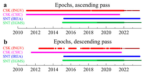
Figure 3.
Dates of the DInSAR displacement time series that we used in this study: (a) ascending-pass time series; (b) descending-pass time series. Same colour palette as in Figure 1.
The dataset comprises 603 ascending-pass and 126 descending-pass epochs for the first period, and 75 ascending-pass and 44 descending-pass epochs for the second period (Figure 3). The first period is hereinafter often referred to as 2011–2021 and the second one as 2021–2023, irrespective of the pass. The time series were produced using GAMMA software (Gamma Remote Sensing AG, Gümligen, Switzerland) [24], which merges the characteristics of the Persistent Scatterers (PS) and Small BAseline Subsets (SBAS) InSAR (Interferometric SAR) techniques. Images were multi-looked to reduce speckle noise. Then, differential interferograms were computed and the topographic phase contribution was removed by using the 12 m digital elevation model (DEM) acquired by the TanDEM-X mission [25]. The resulting interferograms were filtered using a Goldstein filter [26] and unwrapped by the minimum cost flow algorithm [27] with an unwrapping coherence threshold equal to 0.35 (see metadata file at http://www.geosar-iridium.cs.ingv.it, accessed on 14 April 2025); points with temporal coherence greater than 0.5 were retained. Displacement time series were obtained for each point using the algorithm in [28] with added weighted constraints on ground acceleration. An adjustable parameter can be set to a value between 0 and >10 in order to produce a non-smoothed or quasi-linear solution, respectively. This parameter was set to 1.5 to account for non-linear deformation components. Line of sight (LOS) displacement time series are reported for point scatterers identified by their WGS84 geographic coordinates. Displacements are referred to a point close to the cGPS AGR1 station, whose coordinates are 14.343°E, 40.811°N [1].
These data are hereinafter referred to as CSK (INGV). Positions of the measurement points in the region of interest are shown in Figure 1b–d.
CSK (CSIC) Ground Displacement Time Series
The CSK LOS displacement time series in [9] were produced to provide ground displacement data to [23]. A total of 338 images for the ascending pass and 127 images for the descending pass were used. The selected interferometric pairs have a maximum temporal baseline of 96 days with no constraint on the perpendicular baseline. The related interferograms were then generated and unwrapped [29]. Phase contributions due to topography were computed using NASA’s Shuttle Radar Topography Mission (SRTM) 1 arcsec data of the study area [30]. The time series were obtained using the SBAS technique [28]. A temporal coherence threshold [29] of 0.7 was used to select the accepted points. A point located in the centre of Naples (437,175 m E, 4,521,791 m N) was used as the reference point. Finally, the time series were smoothed and interpolated temporally [23]. The resulting ascending-pass time series in [9] consisted of 241 regularly spaced dates ranging from 2009.5554 to 2021.5554 (Figure 3a). The descending-pass time series consists of 204 regularly spaced dates ranging from 2011.5513 to 2021.7013 (Figure 3b). The time step is 18.25 days for both time series. LOS displacement time series are provided for scatterers identified by their UTM WGS84 33N coordinates. The LOS direction cosines relative to the east, north and up directions are also provided for each scatterer.
These data are hereinafter referred to as CSK (CSIC). Positions of the measurement points in the region of interest are shown in Figure 1e,f.
2.1.3. Sentinel-1 Data
The Sentinel-1 constellation is the European radar observatory for Copernicus, a joint initiative of the European Commission and the European Space Agency. Its primary functions are land monitoring, maritime monitoring and emergency management [31].
Three satellites were launched between 2014 and 2024, while one more satellite was launched on 4 November 2025. Each satellite carries a radar instrument operating in the C band. The two-satellite constellation offers a six-day exact repeat cycle; the revisit rate (ascending/descending) spans less than 1 day at the Arctic and within 3 days at the equator. Sentinel-1A and Sentinel-1C remain operational, while the mission ended for Sentinel-1B in 2022; Sentinel-1D will soon replace the older Sentinel-1A satellite. A number of websites, including one operated by the European Space Agency [32], provide all Sentinel-1 (SNT) data, which can be downloaded at no cost.
The set of LOS displacement time series from SNT data in the Campi Flegrei area that we use here have been published by [33] and made freely accessible via the internet [10]. Moreover, time series of ground displacement across most of Europe, and thus, also in the Campi Flegrei area, from SNT images are available through the European Ground Motion Service (EGMS) [11]. This service provides three main InSAR products: Basic, Calibrated and Ortho. The first two products provide displacement data in the satellite LOS, while the third product provides nearly vertical and east–west displacements.
SNT (IREA) Ground Displacement Time Series
Two LOS displacement time series are available for download from [10]: 412 epochs (25 March 2015–21 October 2023) for the ascending pass and 411 epochs (24 March 2015–20 October 2023) for the descending pass (Figure 3). Ascending and descending images (orbits 44 and 22, VV polarization) were processed by IREA-CNR using the Parallel SBAS algorithm [34,35]. The images were co-registered on a burst-by-burst basis to a common reference image [36], then differential interferograms were computed and selected by imposing a maximum temporal baseline of 350 days. The images were flattened by using the 1-arcsec SRTM digital elevation model (DEM) [30], multi-looked and filtered using a Goldstein filter. The differential interferograms were then unwrapped through an extension of the minimum cost flow (EMCF) algorithm [29]. The LOS displacement time series were thus compared with cGPS data; the mean standard deviation of the differences between the two kinds of data is approximately 5 mm [33]. The time series are given over an incomplete regular grid with 1-arcsec spacing; the coordinate reference system is WGS84. Coordinates of the displacement reference points are 14.241264°E, 40.844146°N for the ascending pass and 14.252292°E, 40.833724°N for the descending pass. The LOS direction cosines relative to the east, north and up directions are given for each grid point. Typical incidence angles are close to 36° and 35° for the ascending and descending passes, respectively. The azimuth angles are close to .
This dataset is hereinafter referred to as SNT (IREA). Positions of the measurement points in the region of interest are shown in Figure 1g,h.
SNT (EGMS) Ground Displacement Time Series
The EGMS displacement time series (Figure 3) were obtained from VV-polarized images by employing advanced processing techniques that are based on both the PSI (Persistent Scatterer Interferometry) and DS (Distributed Scatterer Interferometry); the Copernicus GLO-30 (30 m resolution) DEM was used to compensate for the topographic phase contribution; the coordinate reference system is ETRS89-LAEA Europe [37]. A consortium of different InSAR Processing Entities (IPEs) produced the EGMS products. Thus, the processing algorithms implemented in the various processing chains may differ; nevertheless, the end products have analogous attributes and the results are consistent [38].
For the purpose of producing calibrated products, ground displacement is anchored to a reference frame derived from the European GNSS net. The utilisation of GNSS data to calibrate InSAR data renders it nearly independent of the selection of the reference point employed during processing. Moreover, it helps separate true ground movement from sensor or atmospheric artifacts. As a drawback, the EGMS Calibrated products and GNSS data are not independent, and the same holds for the EGMS Ortho products, which are derived from the Calibrated ones [38].
EGMS updates are released periodically. Here we use the first release, which covers the period 2015–2021, and the second release, which covers the period 2019–2023. Comparing two different EGMS releases requires considering that they are independently processed with different estimations, phase unwrapping steps and filters. As a consequence, trends may differ at the end of the overlapping period and, in such a case, the latest release is considered the most reliable. In addition, because of the massive continental-scale data processing, EGMS data is more appropriate for wide-scale analysis, and thus, local deviations cannot be ruled out [39]. The EGMS products include the ETRF89 geographic coordinates, as well as the LOS direction cosines relative to the east, north and up directions for each measurement point.
EGMS time series data are hereinafter referred to as SNT (EGMS). Positions of the measurement points in the region of interest are shown in Figure 1i–l.
2.2. Methods
As stated in Section 2.1, cGPS, CSK (INGV), CSK (CSIC), SNT (IREA) and SNT (EGMS) displacements refer to different points. Unfortunately, we could not use the cGPS local reference frame for the DInSAR time series because the study area does not include the RING stations employed by [1]. We chose not to use any cGPS stations in the Campi Flegrei area as reference points, as these could potentially be affected by deformation phenomena linked with volcanic activity. Instead, we referred the DInSAR displacements to a reference area (Qualiano), which is located at a considerable distance from the deforming Campi Flegrei region and has been highly urbanised for decades. We subtracted the mean displacements of the SAR measurement points within a 200 m radius circle centred on 14.1521°E, 40.9171°N (the yellow square in Figure 1a) from each DInSAR time series.
2.2.1. Comparison Between DInSAR and cGPS Time Series
To compare the DInSAR and cGPS time series, we computed the mean DInSAR LOS displacement for all measurement points within 200 m radius circles centred on each cGPS station. The weekly cGPS ground displacements were projected along each SAR LOS direction by combining the three displacement components— from south to north, from west to east and upward (e.g., [40]). Table 1 summarises the typical values of the parameters describing the LOS directions in the study area.

Table 1.
Parameters describing the LOS directions in the Campi Flegrei area: , and —direction cosines with respect to the east, north and up directions; —angle of incidence; —azimuth.
2.2.2. Quasi-Vertical and Eastward Ground Displacements
As the angles of incidence of the CSK and SNT LOSs are significantly different (see Table 1), it is meaningless to make a direct comparison between the time series of the CSK and SNT LOS displacements. As is standard practice, we calculated the 2.5D (quasi-vertical and eastward ) displacement field [41]. Because measurement points differ between CSK (INGV), CSK (CSIC), SNT (IREA) and SNT (EGMS), the LOS displacement time series for each mission and pass were first estimated on a regular 150 m × 150 m UTM WGS84 33N grid by computing the mean displacement within each non-empty grid cell.
In principle the ascending- and descending-pass time series should share the same observation dates in order to compute the quasi-vertical and eastward displacements. However, exact temporal coincidence is lacking. Given the slow deformation at Campi Flegrei, the LOS time series can be safely interpolated. As the CSK (INGV) descending-pass series has far fewer dates than the others, all time series were interpolated to the CSK (INGV) descending-pass dates. Quasi-vertical and eastward displacements were then computed from the interpolated ascending and descending series for each dataset—CSK (INGV), CSK (CSIC), SNT (IREA) and SNT (EGMS).
3. Results
3.1. Comparison Between CSK and cGPS Time Series, 2011 to 2023
We first compared the CSK (INGV) and CSK (CSIC) LOS displacements with projected cGPS displacements for both the ascending (Figure 4) and descending (Figure 5) passes. Time series were shifted to maximize the overlap between the initial portions of the DInSAR and cGPS records and to connect the 2011–2021 and 2021–2023 CSK (INGV) segments to avoid discontinuities. The differences between the CSK and cGPS displacements (cGPS filtered with a five-week moving average) are shown in Figure 6 and Figure 7 for the ascending and descending passes, respectively.
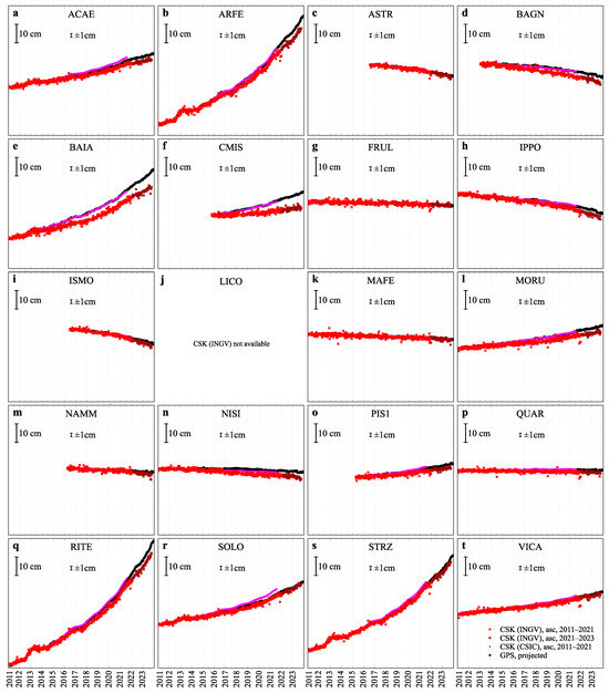
Figure 4.
Comparison between the CSK LOS displacements for the ascending pass (coloured symbols: same colour palette as in Figure 1) and the projected cGPS ones (black dots). Plots (a–t) refer to the cGPS stations in Figure 1a, arranged in alphabetical order. The 2021–2023 CSK (INGV) LOS displacements were shifted in order to align with the final segment of the 2011–2021 CSK (INGV) LOS displacement time series. The time periods during which cGPS data are available are the only periods that are shown for each cGPS station. The scale of the y-axis is indicated in each plot by a black, labelled vertical bar, the length of which corresponds to a 10-cm displacement. A smaller, black, labelled vertical bar indicates typical discrepancies between DInSAR and cGPS LOS displacements at the two-standard-deviation level, i.e., ±1 cm [33].
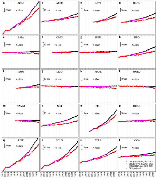
Figure 5.
Comparison between the CSK LOS displacements for the descending pass (coloured symbols: same colour palette as in Figure 1) and the projected cGPS ones (black dots). Plots (a–t) refer to the cGPS stations in Figure 1a, arranged in alphabetical order. The 2021–2023 CSK (INGV) LOS displacements were shifted in order to align with the final segment of the 2012–2021 CSK (INGV) LOS displacement time series. The time periods during which cGPS data are available are the only periods that are shown for each cGPS station. The scale of the y-axis is indicated in each plot by a black, labelled vertical bar, the length of which corresponds to a 10-cm displacement. A smaller, black, labelled vertical bar indicates typical discrepancies between DInSAR and cGPS LOS displacements at the two-standard-deviation level, i.e., ±1 cm [33].
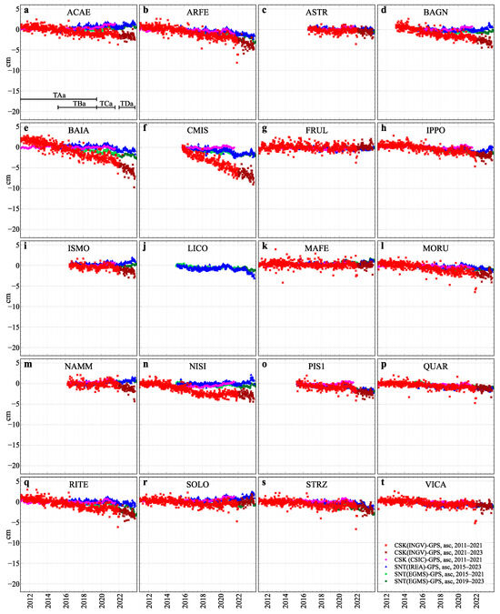
Figure 6.
Differences between DInSAR LOS displacements and projected, filtered cGPS ones for the ascending pass (same colour palette as in Figure 1). The time periods during which cGPS data are available are the only periods that are shown for each cGPS station. The 2021–2023 CSK (INGV) LOS displacements were shifted in order to align with the final segment of the 2011–2021 CSK (INGV) LOS displacement time series. Both the resulting CSK (INGV) and CSK (CSIC) LOS displacements were shifted in order to align with the cGPS displacements in spring 2015, i.e., when the SNT time series commence. The 2019–2023 SNT (EMGS) LOS displacements were shifted in order to align with the overlapping segment of the 2015–2021 SNT (EMGS) LOS displacement time series. Plots (a–t) refer to the cGPS stations indicated in Figure 1a, arranged in alphabetical order. The black segments in (a) identify the time periods TAa, TBa, TCa and TDa, which were used in this work for comparing the mean ascending-pass displacement rates in Section 3.3.
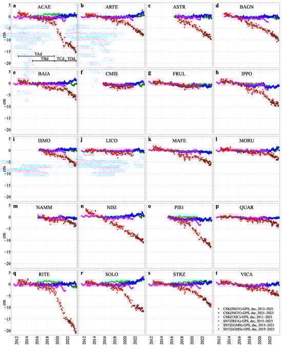
Figure 7.
Differences between DInSAR LOS displacements and projected, filtered cGPS ones in the descending pass (same colour palette as in Figure 1). The time periods during which cGPS data are available are the only periods that are shown for each cGPS station. The 2021–2023 CSK (INGV) LOS displacements were shifted in order to align with the final segment of the 2012–2021 CSK (INGV) LOS displacement time series. Both the resulting CSK (INGV) and CSK (CSIC) LOS displacements were shifted in order to align with the cGPS displacements in spring 2015, i.e., when the SNT time series commenced. The 2019–2023 SNT (EMGS) LOS displacements were shifted in order to align with the overlapping segment of the 2015–2021 SNT (EMGS) LOS displacement time series. Plots (a–t) refer to the cGPS stations indicated in Figure 1a, arranged in alphabetical order. The black segments in (a) identify the time periods TAd, TBd, TCd and TDd, which are used in this work for comparing the mean descending-pass displacement rates in Section 3.3.
For the CSK (INGV) ascending pass, the LOS displacements generally agree with cGPS but are sometimes smaller. The mismatch onset times vary by station; cumulative discrepancies reach ≈5 cm at ARFE and RITE (Figure 4b,f,q and Figure 6b,f,q) and ≈10 cm at BAIA and CMIS (Figure 4e and Figure 6e). The CSK (INGV) descending-pass displacements show substantially poorer agreement: DInSAR values systematically underestimate cGPS, with station-dependent mismatch onset times. Differences reach ≈10 cm at BAGN, IPPO, NISI, SOLO and STRZ (Figure 5d,h,n,r,s and Figure 7d,h,n,r,s), and exceed 20 cm at ACAE and RITE (Figure 5a,q and Figure 7a,q). By contrast, the CSK (CSIC) LOS displacements show good agreement with cGPS for both the ascending and descending passes (Figure 4 and Figure 5).
3.2. Comparison Between SNT and cGPS Time Series, 2015 to 2023
Comparing the SNT (IREA), SNT (EGMS) and cGPS time series allowed us to determine whether other freely available DInSAR displacement time series are in agreement with the projected cGPS data. Unfortunately, this comparison cannot be extended to displacement data preceding 2015.
Figure 8 and Figure 9 show that the SNT (EGMS) and SNT (IREA) displacement time series agree much more closely with cGPS than the CSK (INGV) series. This improved congruence is especially pronounced for the descending passes, as reflected in the DInSAR-cGPS differences plotted in Figure 6 and Figure 7.
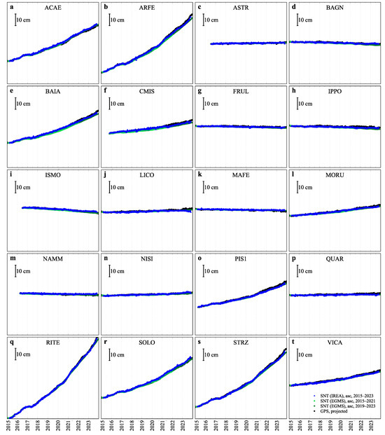
Figure 8.
Comparison between the SNT LOS displacements for the ascending pass (coloured symbols: same colour palette as in Figure 1) and the projected cGPS ones (black dots). Plots (a–t) refer to the cGPS stations in Figure 1a, arranged in alphabetical order. The 2019–2023 SNT (EMGS) LOS displacements were shifted in order to align with the overlapping segment of the 2015–2021 SNT (EMGS) LOS displacement time series. The time periods during which cGPS data are available are the only periods that are shown for each cGPS station. The scale of the y-axis is indicated in each plot by a black, labelled vertical bar, the length of which corresponds to a 10-cm displacement.
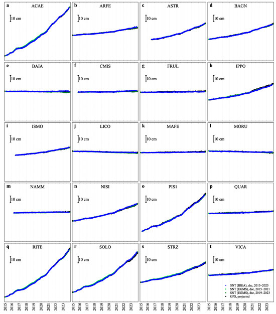
Figure 9.
Comparison between the SNT LOS displacements for the descending pass (coloured symbols: same colour palette as in Figure 1) and the projected cGPS ones (black dots). Plots (a–t) refer to the cGPS stations in Figure 1a, arranged in alphabetical order. The 2019–2023 SNT (EMGS) LOS displacements were shifted in order to align with the overlapping segment of the 2015–2021 SNT (EMGS) LOS displacement time series. The time periods during which cGPS data are available are the only periods that are shown for each cGPS station. The scale of the y-axis is indicated in each plot by a black, labelled vertical bar, the length of which corresponds to a 10-cm displacement.
3.3. Comparison Between DInSAR and cGPS Mean Displacement Rates
The plots in Figure 7 indicate that during the three periods TAd (before July 2019), TCd (July 2019 to September 2021) and TDd (September 2021 to October 2023), the differences between the CSK (INGV) descending-pass LOS displacements and the projected cGPS displacements increase almost linearly over time, albeit at very different rates (see Figure 7a). The TBd period (March 2015 to July 2019) coincides with the period of TAd for which SNT data is also available.
Thus, we calculated the mean displacement rate and its standard deviation for each DInSAR descending-pass displacement time series, as well as for the related projected cGPS displacement time series, using simple chi-squared linear fits (e.g., [42]). This computation was performed for each time period (TAd, TBd, TCd and TDd in Figure 7a) and for each cGPS station for which data covering at least 90% of the considered time period are available. Then, we computed the difference between each DInSAR mean displacement rate and the corresponding cGPS rate. The error of this difference at the two-standard-deviation level was estimated by , where is the standard deviation of the DInSAR mean displacement rate and is the standard deviation of the cGPS rate. The results are plotted in Figure 10. Deformation rates derived from CSK (INGV) data differ most greatly from the cGPS data, particularly during the TCd period (July 2019 to September 2021), with discrepancies reaching values of several cm/year. These discrepancies vary from one period to another, with different time histories for the various stations. The discrepancies for CSK (CSIC), SNT (EGMS) and SNT (IREA) are similar to each other.
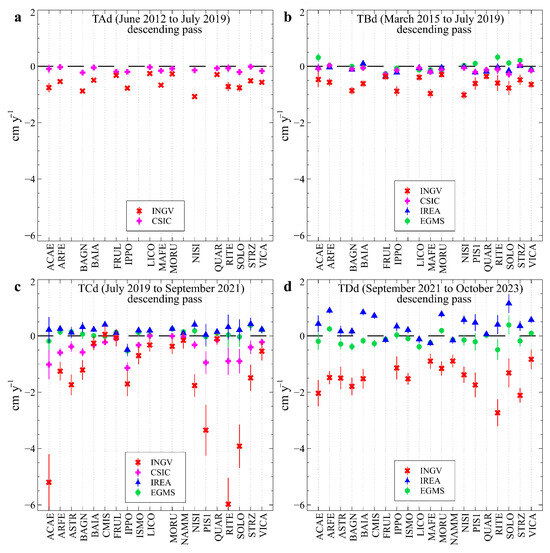
Figure 10.
Mean displacement rate differences between DInSAR and cGPS for four selected time periods (TAd, TBd, TCd and TDd in Figure 7a) for the descending pass. The colour palette is analogous to that in Figure 1. For the SNT (EGMS) time series, the 2015–2021 time series was used for TBd, while the 2019–2023 time series was used for TCd and TDd. The vertical segments overlapping the symbols show uncertainties at the two-standard-deviation level. For clarity, the zero-difference level is indicated by a black, dashed horizontal line. (a) TAd; (b) TBd; (c) TCd; (d) TDd.
We performed the same analysis on the ascending-pass time series. Relative to the corresponding descending-pass intervals, TCa ended two months before TCd to allow for inclusion of the CSK (CSIC) data, while TDa began three months after TDd to avoid merging the two INGV ascending-pass time series (see Figure 3). The results are shown in Figure 11. Unlike for the descending-pass time series, the discrepancies between the ascending-pass time series are all similar.
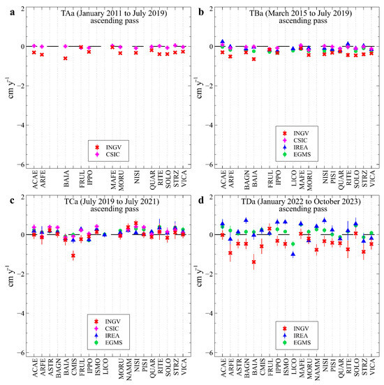
Figure 11.
Mean displacement rate differences between DInSAR and cGPS for four selected time periods (TAa, TBa, TCa and TDa in Figure 6a) for the ascending pass. The colour palette is analogous to that in Figure 1. For the SNT (EGMS) time series, the 2015–2021 time series was used for TBa, while the 2019–2023 time series was used for TCa and TDa. The vertical segments overlapping the symbols show uncertainties at the two-standard-deviation level. For clarity, the zero-difference level is indicated by a black, dashed horizontal line. (a) TAa; (b) TBa; (c) TCa; (d) TDa.
3.4. Quasi-Vertical and Eastward Ground Displacements
We also compared the temporal evolution of the quasi-vertical and eastward displacements obtained from the available datasets up until 2021. This is because we wanted to avoid potential artefacts arising from the connection between the two CSK (INGV) data series, which cover the periods before and after 2021, respectively.
We excluded the SNT (EGMS) series because, as noted in Section 2.1, they are not independent of the cGPS data and are better suited to large-scale analysis; local deviations may therefore persist. The CSK (CSIC) series allowed comparison of CSK-derived ground displacements produced by different authors.
Because SNT (IREA) and CSK (CSIC) agree well with cGPS, comparing CSK (INGV) against CSK (CSIC) and SNT (IREA) let us assess whether the discrepancies between CSK (INGV) and cGPS—and thus, between CSK (INGV) and the “true” ground displacement—arise from time-varying artefacts. Such artefacts could produce apparent, but spurious, changes in the inferred deformation source properties.
First, we calculated the quasi-vertical () and eastward () velocity fields over four time intervals (TA, TB, TC and TD). These intervals are defined by the intersections of TAa and TAd, TBa and TBb, TCa and TCd, and TDa and TDb. Figure 12 and Figure 13 show maps comparing the velocity fields of CSK (INGV) with those of the other time series. For each interval (TA–TD) and each velocity component ( and ), the left map shows the reference velocity field: CSK (CSIC) for TA and SNT (IREA) for TB, TC and TD. The middle map shows the difference between the CSK (CSIC) velocity field and the reference velocity field. The right map shows the difference between CSK (INGV) and the reference velocity field.
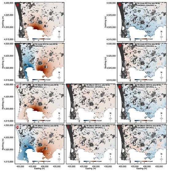
Figure 12.
Maps of the quasi-vertical and horizontal velocities over TA and TB: (a) CSK (CSIC) quasi-vertical velocity over TA; (b) quasi-vertical velocity difference between CSK (INGV) and CSK (CSIC) over TA; (c) CSK (CSIC) eastward velocity over TA; (d) eastward velocity difference between CSK (INGV) and CSK (CSIC) over TA; (e) SNT (IREA) quasi-vertical velocity over TB; (f) quasi-vertical velocity difference between CSK (CSIC) and SNT (IREA) over TB; (g) quasi-vertical velocity difference between CSK (INGV) and SNT (IREA) over TB; (h) SNT (IREA) eastward velocity over TB; (i) eastward velocity difference between CSK (CSIC) and SNT (IREA) over TB; (j) eastward velocity difference between CSK (INGV) and SNT (IREA) over TB. UTM WGS83 33N coordinates.
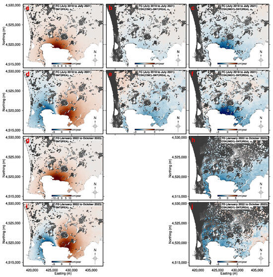
Figure 13.
Maps of the quasi-vertical and horizontal velocities over TC and TD: (a) SNT (IREA) quasi-vertical velocity over TC; (b) quasi-vertical velocity difference between CSK (CSIC) and SNT (IREA) over TC; (c) quasi-vertical velocity difference between CSK (INGV) and SNT (IREA) over TC; (d) SNT (IREA) eastward velocity over TC; (e) eastward velocity difference between CSK (CSIC) and SNT (IREA) over TC; (f) eastward velocity difference between CSK (INGV) and SNT (IREA) over TC; (g) SNT (IREA) quasi-vertical velocity over TD; (h) quasi-vertical velocity difference between CSK (INGV) and SNT (IREA) over TD; (i) SNT (IREA) eastward velocity over TD; (j) eastward velocity difference between CSK (INGV) and SNT (IREA) over TD. UTM WGS83 33N coordinates.
As Figure 6 and Figure 7 suggest, there are particularly large discrepancies between CSK (INGV) and the reference velocity map during TC and TD (Figure 13). When all three datasets are available—CSK (INGV), CSK (CSIC) and SNT (IREA)—it is consistently the CSK (INGV) velocity field that differs the most from the reference map. The discrepancies for the CSK (INGV) velocity vary depending on the time interval and velocity component in terms of both the spatial pattern and magnitude.
The Supplementary Information Videos S1–S4 relate to the quasi-vertical and eastward ground displacements at each CSK (INGV) descending-pass epoch. Video S1 shows the pixel-wise difference between the CSK (INGV) and CSK (CSIC) time series between 2012 and 2021. Video S2 shows the pixel-wise difference between the CSK (INGV) and CSK (CSIC) time series between 2015 and 2021. Video S3 shows the pixel-wise difference between the CSK (INGV) and SNT (IREA) time series between 2015 and 2021. Video S4 shows the pixel-wise difference between the CSK (CSIC) and SNT (IREA) time series between 2015 and 2021. Light yellow pixels denote differences that are smaller than 1 cm. This threshold is twice the mean standard deviation of the differences between SNT (IREA) LOS displacements and cGPS ones [33]. The initial frame, dated 17 October 2015, serves as a reference; consequently, all pixel values are set to 0.
The displacement differences between CSK (INGV) and CSK (CSIC), as well as between CSK (INGV) and SNT (IREA), exhibit significant temporal variation in both the quasi-vertical and eastward components, consistent with the patterns shown in Figure 12 and Figure 13. In contrast, the differences between CSK (CSIC) and SNT (IREA) remain consistently below 1 cm throughout most of the time series, except for the last three epochs. These final discrepancies may result from edge effects associated with the smoothing and interpolation methods employed in generating the CSK (CSIC) time series [9].
4. Discussion
In this paper, we analysed the accuracy of the DInSAR ground displacement time series underlying the purported evidence of recent upward migration and shape changes of magmatic bodies at Campi Flegrei. Needless to say that these results have an obvious impact on the understanding of the physical processes that drive the current unrest phase.
Analysis of CSK (INGV) data by [5] identified a striking temporal evolution in the shape of ground deformation between 2012 and 2023. The analysis of ground deformation in [5] was primarily based on the mean ground displacement rate in the LOS directions during six selected time periods (T2a–T7a and T2d–T7d for the ascending and descending-pass time series, respectively; see Figure 2b). The mean ascending- and descending-pass LOS velocities of each period (e.g., T2a and T2d) were jointly modelled using an 8 km-deep tabular deflating source and a shallow inflating ellipsoidal point source embedded in a heterogeneous, flat medium. The shallower source, whose axes are fixed in the east–west, north–south, and vertical orientations, is represented by the equivalent moment tensor. This shallower source gradually ascended from 5.5 km to 3.9 km, progressively changing shape. It transitioned from a 5.5 km deep circular horizontal sill (T2); to a 5.1 km deep, nearly spheroidal horizontal source with thick prolate geometry (T3); to a 3.9 km deep, nearly spheroidal horizontal source with thin prolate geometry (T4); then to a 3.9 km deep, thick, oblate spheroidal horizontal source (T5); followed by a 3.9 km deep thick, prolate, almost spheroidal horizontal source (T6 and T7). This non-stationary inflating source has been interpreted as being linked to the upward migration of magma.
This overall picture is markedly inconsistent with the outcomes of ground deformation models that were carried out independently using different DInSAR datasets. For example, analysis of SNT data from 2015 to 2022 yielded a stationary ground deformation field that is consistent with two finite sill-like inflating sources embedded in a layered medium, with one shallow (3–4 km) and one deep (approximately 8–9 km) [7]. The shallow source is similar to that responsible for the large-scale deformation field during the uplift from 1982 to 1984 and the subsequent subsidence, which ended around 2000 [7,43,44]. A preliminary analysis of RADARSAT-2 data appears to confirm the stationarity of the deformation field during 2010–2015 [8]. In the analysis of the CSK (CSIC) and, when available, SNT data from 2011 to 2022 made by [23], the deformation field was modelled using a regularised combination of pressure and dislocation sources. It was found that most deformation is attributable to a pressure source whose centre is always at a depth of 2.5–3 km (see Figures 7–14 in [23]).
To gain new insights that may explain these differences, we examined the expected similarity between the ground displacement time series obtained from CSK and SNT imagery and the available cGPS ground deformation data at Campi Flegrei. Our careful analysis revealed a pronounced discrepancy between the ground deformation data from the CSK (INGV) descending-pass time series used by [5] and cGPS measurements. Specifically, differences in the deformation velocity can reach approximately 6 cm/year, with cumulative displacement discrepancies exceeding 20 cm during 2020–2023. These discrepancies exhibit a clear, variable spatial and temporal distribution.
Conversely, the ground deformation time series obtained from the CSK (CSIC), SNT (IREA), SNT (EGMS) and cGPS data over the same region and comparable time interval are fully consistent, as expected if these three DInSAR datasets and cGPS data accurately represent the overall space-time evolution of the ground deformation. The different results obtained from analysing data from the same satellite (CSK) over the same region and comparable time interval using different methodologies [6,9] highlight the sensitivity of these methods and their parameterisations in deriving reliable ground deformation time series. Here, we do not explore this topic in greater detail, as it has been discussed extensively elsewhere [45].
The large INGV (CSK) descending-pass discrepancies could also be due to phase unwrapping errors. To verify this, the congruity of all the triangular loops in the interferometric pairs of the series could be automatically checked a posteriori before producing the time series (e.g., [46]). Atmospheric delays, orbital errors and decorrelation could also be important factors. Unfortunately, it is not possible to obtain more precise information about the discrepancies solely from the analysis of the final time series.
Nonetheless, we argue that the modelling of CSK (INGV) to infer an upward magma migration is based on unreliable time series of the ground deformation. In particular, although the DInSAR phase from X-band images (like CSK) is more affected by decorrelation noise artefacts than that from C-band images (like SNT) (e.g., [23]), the discrepancy between the CSK (INGV) descending-pass data and the cGPS data is much greater than that expected for the DInSAR time series (e.g., [41,45]). This discrepancy can explain the seeming significant “non-stationarity” of the ground deformation field, which is the main empirical evidence to support an upward magma migration [5]. Conversely, the good agreement between SNT (IREA), SNT (EGMS), CSK (CSIC) and GPS data appears to support the conclusion that the shape of the Campi Flegrei deformation field remains almost constant over time within the DInSAR errors [7,8,43,47].
In the near future, we plan to use deformation data from ERS/Envisat, RADARSAT-2, CSK and SNT SAR images to detect any variations in the shape of the Campi Flegrei deformation field that are greater than the margin of error. However, the actual ground deformation is unknown, and it can be challenging to assign realistic uncertainties to deformation measurements. Even when errors arising from the unwrapping process are absent from individual interferograms, the phases still contain contributions from sources other than ground deformation, such as atmospheric and topographic sources, which cannot be completely eliminated. Displacement values obtained from DinSAR time series depend on the details of the applied procedure, whether based on PS, SBAS or variants thereof. Typically, uncertainty in DInSAR data is determined by comparing it with the cGPS (or GNSS) data. The estimated DInSAR error is usually around 5 mm (e.g., [41]). This approach implicitly assumes that cGPS data perfectly reflect true ground deformation. However, cGPS data are also subject to error. For the cGPS series used here, ref. [19] provided a formal error of 1 mm for the horizontal components and 3 mm for the vertical component. Larger errors in cGPS observations may be caused by local noise. Consistency between cGPS and DInSAR data is also important for validating the former. For example, this was performed by [33] in the case of the recent geodetic anomaly in the area of the ACAE cGPS station.
When deformation data from multiple measurement techniques or different processing methodologies are available, a comprehensive comparison can help to identify unreliable data. For example, the CSK (INGV) descending-pass time series was identified as such in this study. In the case of Campi Flegrei specifically, the consistency observed between SNT (IREA), SNT (EGMS), CSK (CSIC) and cGPS data indirectly validates the fact that these measurements are largely free from significant errors. Additionally, it suggests that the reference point chosen for the DInSAR displacements (Qualiano, Figure 1a) can effectively be considered fixed relative to the local reference system used for the cGPS displacements [1]. This makes Qualiano a valuable reference point for analysing ground deformation at Campi Flegrei.
In order to make a thorough comparison of the quality of different data and the related uncertainties, it is crucial that publications transparently detail the methods used to generate the time series and analyse the sensitivity of the results to various parameters (e.g., [45]). As a matter of fact, overly optimistic estimates of error or neglecting uncertainty altogether can lead to misinterpretation and over-modelling of data. Such pitfalls are not limited to SAR data but can also affect GPS measurements, where local environmental noise may be mistaken for genuine deformation signals (e.g., [48]).
5. Conclusions
This paper evaluates the accuracy of DInSAR time series underpinning claims of upward magma migration and changing deformation source geometry at Campi Flegrei. We demonstrate that these time series, which were obtained from COSMO-SkyMed imagery, are inconsistent with cGPS observations. Consequently, the claims of [5] concerning the recent, rapid ascent of a magmatic body are not supported by the evidence. In contrast, independent time series obtained from COSMO-SkyMed and Sentinel-1 imagery, which are consistent with cGPS observations, suggest that the deformation source has remained nearly stationary throughout the ongoing unrest phase.
Our findings advance the debate on the mechanisms driving the current unrest at Campi Flegrei—an area of high volcanic risk and dense population—and may inform volcanic risk assessments and future recommendations by the Major Risks Commission.
Supplementary Materials
The following supporting information can be downloaded from https://www.mdpi.com/article/10.3390/rs17223777/s1: Video S1. Pixel-wise difference between the CSK (INGV) and CSK (CSIC) time series between 2012 and 2021; Video S2. Pixel-wise difference between the CSK (INGV) and CSK (CSIC) time series between 2015 and 2021; Video S3. Pixel-wise difference between the CSK (INGV) and SNT (IREA) time series between 2015 and 2021; Video S4. Pixel-wise difference between the CSK (CSIC) and SNT (IREA) time series between 2015 and 2021.
Author Contributions
Conceptualization, A.A. and L.C.; methodology, A.A. and L.C.; formal analysis, A.A. and L.C.; investigation, A.A. and L.C.; writing—original draft preparation, A.A., W.M. and L.C.; writing—review and editing, A.A., W.M. and L.C.; visualization, A.A., W.M. and L.C.; supervision, L.C. All authors have read and agreed to the published version of the manuscript.
Funding
This research received no external funding.
Data Availability Statement
The ground displacement data used in this study were derived from the following resources available in the public domain: cGPS weekly positions time series, https://zenodo.org/records/10082466 (accessed on 11 July 2025); CSK (INGV) time series, http://www.geosar-iridium.ct.ingv.it/landing/ts_page.php/ (accessed on 16 November 2025); CSK (CSIC) time series, https://digital.csic.es/handle/10261/341157/ (accessed on 22 August 2025); SNT (IREA) time series, https://zenodo.org/records/10781496/ (accessed on 15 April 2025); SNT (EGMS) time series, https://land.copernicus.eu/en/products/european-ground-motion-service (accessed on 14 April 2025). TINITALY/01 DEM can be downloaded from http://tinitaly.pi.ingv.it/ (accessed on 11 July 2025). In case of difficulties downloading CSK(INGV) data, the authors of this article will make it available on request.
Acknowledgments
We would like to express our gratitude to the authors and maintainers of the open-source software used for this study, including GMT (https://www.generic-mapping-tools.org/, accessed on 23 July 2025), Veusz (https://veusz.github.io/, accessed on 23 July 2025), LibreOffice (https://libreoffice.org, accessed on 23 July 2025), and Inkscape (https://inkscape.org/, accessed on 16 November 2025).
Conflicts of Interest
The authors declare no conflicts of interest.
Abbreviations
The following abbreviations are used in this manuscript:
| SAR | Synthetic aperture radar |
| SBAS | Small BAseline Subset |
| DInSAR | Differential Synthetic Aperture Radar Interferometry |
| LOS | Line of sight |
| DEM | Digital elevation model |
| cGPS | continuous Global Positioning System |
| GNSS | Global Navigation Satellite System |
| CSIC | Consejo Superior de Investigaciones Científicas |
| INGV | Istituto Nazionale di Geofisica e Vulcanologia |
| IREA | Istituto per il Rilevamento Elettromagnetico dell’Ambiente |
| NeVoCGPS | Neapolitan Volcanoes Continuous GPS network |
| ESA | European Space Agency |
| ASI | Agenzia Spaziale Italiana |
References
- De Martino, P.; Dolce, M.; Brandi, G.; Scarpato, G.; Tammaro, U. The Ground Deformation History of the Neapolitan Volcanic Area (Campi Flegrei Caldera, Somma–Vesuvius Volcano, and Ischia Island) from 20 Years of Continuous GPS Observations (2000–2019). Remote Sens. 2021, 13, 2725. [Google Scholar] [CrossRef]
- Dipartimento della Protezione Civile. Percorso per l’Aggiornamento del Piano Nazionale di Protezione Civile per i Campi Flegrei. 2019. Available online: https://www.protezionecivile.gov.it/it/approfondimento/il-percorso-laggiornamento-del-piano-nazionale-di-protezione-civile-i-campi-flegrei-0/ (accessed on 3 November 2025).
- Iervolino, I.; Cito, P.; De Falco, M.; Festa, G.; Herrmann, M.; Lomax, A.; Marzocchi, W.; Santo, A.; Strumia, C.; Massaro, L.; et al. Seismic Risk Mitigation at Campi Flegrei in Volcanic Unrest. Nat. Commun. 2024, 15, 10474. [Google Scholar] [CrossRef] [PubMed]
- Tan, X.; Tramelli, A.; Gammaldi, S.; Beroza, G.C.; Ellsworth, W.L.; Marzocchi, W. A clearer view of the current phase of unrest at Campi Flegrei caldera. Science 2025, 390, 70–75. [Google Scholar] [CrossRef] [PubMed]
- Astort, A.; Trasatti, E.; Caricchi, L.; Acocella, V.; Di Vito, M.A. Tracking the 2007–2023 magma-driven unrest at Campi Flegrei caldera (Italy). Commun. Earth Environ. 2024, 5, 506. [Google Scholar] [CrossRef]
- InSAR Working Group—INGV. InSAR Ground Displacement Time Series. 2022. Available online: http://www.geosar-iridium.ct.ingv.it/landing/ts_page.php/ (accessed on 22 October 2025).
- Amoruso, A.; Crescentini, L. Clues of Ongoing Deep Magma Inflation at Campi Flegrei Caldera (Italy) from Empirical Orthogonal Function Analysis of SAR Data. Remote Sens. 2022, 14, 5698. [Google Scholar] [CrossRef]
- Amoruso, A.; Salicone, G.; Crescentini, L. Campi Flegrei and Vesuvio, Italy: Ground Deformation between ERS/ENVISAT and Sentinel-1 Missions from RADARSAT-2 Imagery. Remote Sens. 2025, 17, 3268. [Google Scholar] [CrossRef]
- Tizzani, P.; Camacho, A.G.; Vitale, A.; Escayo, J.; Barone, A.; Castaldo, R.; Pepe, S.; De Novellis, V.; Solaro, G.; Pepe, A.; et al. Dataset of the manuscript “4D Imaging of the Volcano Feeding System beneath the Urban Area of the Campi Flegrei Caldera”. Digital.CSIC, 2024. Available online: https://digital.csic.es/handle/10261/341157 (accessed on 22 August 2025).
- Giudicepietro, F.; Casu, F.; Bonano, M.; De Luca, C.; De Martino, P.; Di Traglia, F.; Di Vito, M.; Macedonio, G.; Manunta, M.; Monterroso, F.; et al. Geodetic Anomaly Detection and Analysis in the Campi Flegrei Caldera (Italy) Deformation Pattern of the 2021–2023 Escalating Unrest Phase. 2024. Available online: https://zenodo.org/records/10781496 (accessed on 16 November 2025).
- European Ground Motion Service. 2025. Available online: https://land.copernicus.eu/en/products/european-ground-motion-service/ (accessed on 22 May 2025).
- Polcari, M.; Borgstrom, S.; Del Gaudio, C.; De Martino, P.; Ricco, C.; Siniscalchi, V.; Trasatti, E. Thirty years of volcano geodesy from space at Campi Flegrei caldera (Italy). Sci. Data 2022, 9, 728. [Google Scholar] [CrossRef]
- Tarquini, S.; Isola, I.; Favalli, M.; Battistini, A.; Dotta, G. TINITALY, a Digital Elevation Model of Italy with a 10 Meters Cell Size (Version 1.1). Istituto Nazionale di Geofisica e Vulcanologia (INGV). 2023. Available online: https://tinitaly.pi.ingv.it/ (accessed on 16 November 2025).
- Del Gaudio, C.; Aquino, I.; Ricciardi, G.; Ricco, C.; Scandone, R. Unrest episodes at Campi Flegrei: A reconstruction of vertical ground movements during 1905–2009. J. Volcanol. Geotherm. Res. 2010, 185, 48–56. [Google Scholar] [CrossRef]
- Sezione di Napoli OSSERVATORIO VESUVIANO. Bollettino di Sorveglianza—CAMPI FLEGREI—APRILE, 2025. Available online: https://www.ov.ingv.it/index.php/monitoraggio-e-infrastrutture/bollettini-tutti/mensili-dei-vulcani-della-campania/flegrei/ (accessed on 22 May 2025).
- Dvorak, J.J.; Berrino, G. Recent ground movement and seismic activity in Campi Flegrei, southern Italy, episodic growth of a resurgent dome. J. Geophys. Res. 1991, 96, 2309–2323. [Google Scholar] [CrossRef]
- Sansosti, E.; Berardino, P.; Bonano, M.; Calò, F.; Castaldo, R.; Casu, F.; Manunta, M.; Manzo, M.; Pepe, A.; Pepe, S.; et al. How second generation SAR systems are impacting the analysis of ground deformation. Int. J. Appl. Earth Obs. Geoinf. 2014, 28, 1–11. [Google Scholar] [CrossRef]
- Tiampo, K.F.; González, P.J.; Samsonov, S.; Fernández, J.; Camacho, A. Principal component analysis of MSBAS DInSAR time series from Campi Flegrei, Italy. J. Volcanol. Geotherm. Res. 2017, 344, 139–153. [Google Scholar] [CrossRef]
- De Martino, P.; Dolce, M.; Brandi, G.; Scarpato, G. Campi Flegrei cGPS Weekly Positions Time Series. 2023. Available online: https://zenodo.org/records/10082466/ (accessed on 22 May 2025).
- INGV RING Working Group. Rete Integrata Nazionale GPS (RING). 2016. Available online: https://webring.gm.ingv.it/ (accessed on 16 November 2025).
- ASI. COSMO-SKYMED, 2025. Available online: https://www.asi.it/en/earth-science/cosmo-skymed/ (accessed on 22 May 2025).
- Group on Earth Observations. Vesuvius—Campi Flegrei Supersite, 2025. Available online: https://geo-gsnl.org/supersites/permanent-supersites/vesuvius-campi-flegrei-supersite/ (accessed on 22 May 2025).
- Tizzani, P.; Fernández, J.; Vitale, A.; Escayo, J.; Barone, A.; Castaldo, R.; Pepe, S.; De Novellis, V.; Solaro, G.; Pepe, A.; et al. 4D imaging of the volcano feeding system beneath the urban area of the Campi Flegrei caldera. Remote Sens. Environ. 2024, 315, 114480. [Google Scholar] [CrossRef]
- Wegmuller, U.; Werner, C. Gamma SAR processor and interferometry software. In Proceedings of the ERS Symposium on Space at the Service of Our Environment, Florence, Italy, 17–21 March 1997; pp. 1687–1692. [Google Scholar]
- German Aerospace Center (DLR). TanDEM-X Science Service System. 2025. Available online: https://tandemx-science.dlr.de/ (accessed on 3 November 2025).
- Goldstein, R.M.; Werner, C.L. Radar Interferogram Phase Filtering for Geophysical Applications. Geophys. Res. Lett. 1998, 25, 4035–4038. [Google Scholar] [CrossRef]
- Costantini, M. A novel phase unwrapping method based on network programming. IEEE Trans. Geosci. Remote Sens. 1998, 36, 813–821. [Google Scholar] [CrossRef]
- Berardino, P.; Fornaro, G.; Lanari, R.; Sansosti, E. A new algorithm for surface deformation monitoring based on small baseline differential SAR interferograms. IEEE Trans. Geosci. Remote Sens. 2002, 40, 2375–2383. [Google Scholar] [CrossRef]
- Pepe, A.; Lanari, R. On the extension of the minimum cost flow algorithm for phase unwrapping of multitemporal differential SAR interferograms. IEEE Trans. Geosci. Remote Sens. 2006, 44, 2374–2383. [Google Scholar] [CrossRef]
- Shuttle Radar Topography Mission (SRTM). Available online: https://www.earthdata.nasa.gov/data/instruments/srtm (accessed on 8 July 2025).
- Sentinel-1, Radar Vision for Copernicus. Available online: https://www.esa.int/Applications/Observing_the_Earth/Copernicus/Sentinel-1 (accessed on 22 May 2025).
- Explore Data. Available online: https://dataspace.copernicus.eu/explore-data (accessed on 22 May 2025).
- Giudicepietro, F.; Casu, F.; Bonano, M.; De Luca, C.; De Martino, P.; Di Traglia, F.; Di Vito, M.; Macedonio, G.; Manunta, M.; Monterroso, F.; et al. First evidence of a geodetic anomaly in the Campi Flegrei caldera (Italy) ground deformation pattern revealed by DInSAR and GNSS measurements during the 2021–2023 escalating unrest phase. Int. J. Appl. Earth Obs. Geoinf. 2024, 132, 104060. [Google Scholar] [CrossRef]
- Casu, F.; Elefante, S.; Imperatore, P.; Zinno, I.; Manunta, M.; De Luca, C.; Lanari, R. SBAS-DInSAR parallel processing for deformation time-series computation. IEEE J. Sel. Top. Appl. Earth Obs. Remote Sens. 2014, 7, 3285–3296. [Google Scholar] [CrossRef]
- Manunta, M.; De Luca, C.; Zinno, I.; Casu, F.; Manzo, M.; Bonano, M.; Fusco, A.; Pepe, A.; Onorato, G.; Berardino, P.; et al. The Parallel SBAS Approach for Sentinel-1 Interferometric Wide Swath Deformation Time-Series Generation: Algorithm Description and Products Quality Assessment. IEEE Trans. Geosci. Remote Sens. 2019, 57, 6259–6281. [Google Scholar] [CrossRef]
- Sansosti, E.; Berardino, P.; Manunta, M.; Serafino, F.; Fornaro, G. Geometrical SAR image registration. IEEE Trans. Geosci. Remote Sens. 2006, 44, 2861–2870. [Google Scholar] [CrossRef]
- Costantini, M.; Minati, F.; Trillo, F.; Ferretti, A.; Passera, E.; Rucci, A.; Dehls, J.; Larsen, Y.; Marinkovic, P.; Eineder, M.; et al. EGMS: Europe-Wide Ground Motion Monitoring based on Full Resolution Insar Processing of All Sentinel-1 Acquisitions. In Proceedings of the 2022 IEEE International Geoscience and Remote Sensing Symposium IGARSS, Kuala Lumpur, Malaysia, 17–22 July 2022; pp. 5093–5096. [Google Scholar] [CrossRef]
- Algorithm Theoretical Basis Document—European Ground Motion Service. Available online: https://land.copernicus.eu/en/products/european-ground-motion-service?tab=documentation (accessed on 8 July 2025).
- EGMS Frequently Asked Questions. Available online: https://land.copernicus.eu/en/faq/products/european-ground-motion-service (accessed on 8 July 2025).
- Fuhrmann, T.; Garthwaite, M.C. Resolving Three-Dimensional Surface Motion with InSAR: Constraints from Multi-Geometry Data Fusion. Remote Sens. 2019, 11, 241. [Google Scholar] [CrossRef]
- Pepe, A.; Calò, F. A review of interferometric Synthetic Aperture RADAR (InSAR) multi-track approaches for the retrieval of Earth’s surface displacements. Appl. Sci. 2017, 7, 1264. [Google Scholar] [CrossRef]
- Press, W.H.; Teukolsky, S.A.; Vetterling, W.T.; Flannery, B.P. NUMERICAL RECIPES—The Art of Scientific Computing, 3rd ed.; Cambridge University Press: New York, NY, USA, 2007; ISBN 9780521880688. [Google Scholar]
- Amoruso, A.; Crescentini, L.; Sabbetta, I. Paired deformation sources of the Campi Flegrei caldera (Italy) required by recent (1980–2010) deformation history. J. Geophys. Res. Solid Earth 2014, 119, 858–879. [Google Scholar] [CrossRef]
- Amoruso, A.; Crescentini, L.; Sabbetta, I.; De Martino, P.; Obrizzo, F.; Tammaro, U. Clues to the cause of the 2011–2013 Campi Flegrei caldera unrest, Italy, from continuous GPS data. Geophys. Res. Lett. 2014, 41, 3081–3088. [Google Scholar] [CrossRef]
- Balz, T.; Ewais, M. Influence of Parameter Estimation Bounds on Velocity Estimation in PSInSAR. Remote Sens. 2025, 17, 788. [Google Scholar] [CrossRef]
- Xu, X.; Sandwell, D.T. Toward Absolute Phase Change Recovery With InSAR: Correcting for Earth Tides and Phase Unwrapping Ambiguities. IEEE Trans. Geosci. Remote Sens. 2020, 58, 726–733. [Google Scholar] [CrossRef]
- Matano, F.; Casaburi, A.; De Natale, G. An MT-InSAR-Based Procedure for Detecting and Interpreting Vertical Ground Deformation Anomalies During Phases of Unrest at Campi Flegrei Caldera, Italy. Appl. Sci. 2025, 15, 3344. [Google Scholar] [CrossRef]
- Amoruso, A.; Crescentini, L.; Chiaraluce, L. Surface temperature and precipitation affecting GPS signals before the 2009 L’Aquila earthquake (Central Italy). Geophys. J. Int. 2017, 210, 911–918. [Google Scholar] [CrossRef]


Disclaimer/Publisher’s Note: The statements, opinions and data contained in all publications are solely those of the individual author(s) and contributor(s) and not of MDPI and/or the editor(s). MDPI and/or the editor(s) disclaim responsibility for any injury to people or property resulting from any ideas, methods, instructions or products referred to in the content. |
© 2025 by the authors. Licensee MDPI, Basel, Switzerland. This article is an open access article distributed under the terms and conditions of the Creative Commons Attribution (CC BY) license (https://creativecommons.org/licenses/by/4.0/).