Highlights
What are the main findings?
- Demonstration of how the dual-frequency reference technique links sigma0 data from multiple altimeter missions.
- Sigma0 values affected by both environmental factors and processing choices.
What are the implications of the main findings?
- Long-term consistency in altimeter record is achieved, enabling more robust trend analysis of winds.
- Better calculation of wave period, sea state bias and gas transfer velocities for climate studies is enabled.
Abstract
Radar altimeters receive radio-wave reflections from nadir and determine surface parameters from the strength and shape of the return signal. Over the oceans, the strength of the return, termed sigma0 (), is strongly related to the small-scale roughness of the ocean surface and is used to estimate near-surface wind speed. However, a number of other factors affect , and these need to be estimated and compensated for when developing long-term consistent records spanning multiple missions. Aside from unresolved issues of absolute calibration, there are various geophysical factors (sea surface temperature, wave height and rain) that have an effect. The choice of the waveform retracking algorithm also affects the values, with the four-parameter Maximum Likelihood Estimator introducing a strong dependence on waveform-derived mispointing and the use of delay-Doppler processing leading to apparent variation with spacecraft radial velocity. As all of these terms have strong geographical correlations, care is required to disentangle these various effects in order to establish a long-term consistent record. This goal will enable a better investigation of the long-term changes in wind speed at sea.
1. Introduction
Spaceborne radar altimeters emit a series of radio-wave pulses and record their reflection from nadir points on the Earth’s surface. The conventional processing of the return echo characterises the signal in terms of amplitude (signal strength), position (time delay before reception) and shape. The latter term may be interpreted over the ocean as significant wave height (Hs), satellite mispointing () and skewness of the sea surface distribution [1,2].
Over the Greenland and Antarctic ice caps, the shape of the return may be influenced by the compactness and dampness of snow and layering within it [3,4,5], and in sea-ice regions, these radar waveforms have to be individually classified to determine whether the reflections are from sea ice or leads within it [6]. Depending upon altimeter altitude and radar operating parameters, the effective surface footprint is a disc of order 7 km across [7,8]; consequently, radar returns from rivers, small lakes and marine coastal zones may include contributions from surfaces with significantly different reflective properties and thus produce more complicated waveforms necessitating specialist interpretation [9,10].
This paper focuses on the amplitude of the signal, which is described by the normalised backscatter coefficient, (where the superscript term emphasises that this relates to incidence angles of 0°), with a particular focus on factors that affect the long-term intercalibration of instruments. The reflectivity of a surface is characteristic of the mismatch in impedances and the roughness of the surface at the appropriate scales. When considering oceanic returns, virtually all the radar signal is reflected, but the angular distribution will depend upon the degree of coherence at lengths similar to the radar wavelength. For oblique-looking systems, such as scatterometers and synthetic aperture radars, a smooth surface reflects radiation away from the direction of the satellite, and increasing roughness causes more of the signal to return to the sensor.
Conversely, for nadir-viewing altimeters, a calm mirror-like surface gives a very strong return and increasing roughness reduces the direct echo. Consequently, the values over the ocean are often used as an indication of wind speed, with a number of heuristic monotonic algorithms being proposed [11,12]. These are often designed or “tuned” for individual altimeters, although a universal form between reflectivity and the geophysical parameter of interest (wind speed) might be expected. Abdalla [13] was a keen proponent of correcting all measurements for instrumental biases and then applying a single wind speed algorithm (see Figure 1) to all. This is particularly a focus of long-term studies looking into climate change [14,15] as the records from many partially overlapping altimeters have to be stitched together. Further studies have suggested that wind speed estimates can be improved by also including wave height as an input to the algorithm [16].
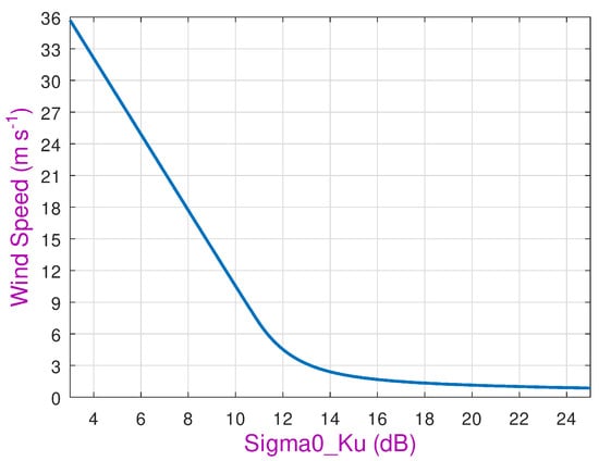
Figure 1.
Wind speed algorithm advocated by Abdalla [13].
The European Space Agency has been supporting the Climate Change Initiative (CCI) to help develop long-term consistent satellite-based datasets of Essential Climate Variables [17] in order to address questions about the trends and long-term variability in these key indicators of the Earth’s health. In its first phase of the Sea State CCI, the emphasis was on the consistency of the wave height record [18]; in the second phase, wind speed and other wave parameters are also being considered. This paper examines the many factors, both instrumental and geophysical, affecting the long-term record, which underpins such studies of wind speed. It builds on the work first advocated by Quartly [19] to use the near-constancy of dual-frequency relationships to drive down the errors in in current altimeter datasets. Section 2 describes the data and methodology for deriving , through both retracking of waveforms and the correction for instrumental factors. Section 3 first provides a comparison of different estimates from the same altimeter and then reviews the dual-frequency technique. Section 3 then looks at a number of factors affecting the precision of that technique, and Section 4 shows how geographic correlations may complicate the interpretation of individual factors. These ideas are brought together in the discussion in Section 5, which includes illustrative applications, with a brief conclusion provided in Section 6.
2. Data and Methodology
2.1. Data Sources
This paper concerns the various factors, related to both geophysical conditions and the processing chain, which affect estimates of sigma0, and how these factors may appear to interact. Table 1 lists the various dual-frequency altimeters used in this paper, along with the data version and their source. Many of these results could be demonstrated for any of the dual-frequency altimeters, or for different processing versions, as there is usually little change to the sigma0 values between different versions of the data. The majority of plots simply use data from Jason-3, as it appears the most stable of all these high-quality missions, but the other missions have also been analysed, giving similar results.

Table 1.
Altimeter data sources and processing. (GDR is geophysical data record, and PLRM is pseudo-low-resolution mode, because the pulse timing of the Sentinel-3 instruments did not allow full LRM processing.)
Over the span of 30 years, there have been many evolutions in the design of altimeter architecture and processing. The earlier instruments simply recorded the sum of many return pulses as a function of time, known as “low-resolution mode” (LRM). Over a uniform surface, such as the ocean, this created a waveform (power return as a function of time) as shown in Figure 2a. Key marine parameters are obtained by “retracking”, i.e., fitting a simple model to the observed shape. The simplest model was MLE-3, a Maximum Likelihood Estimator fitting three parameters (range, wave height and amplitude). Amarouche et al. [20] developed the MLE-4, which fitted a fourth parameter, termed “mispointing”; this could be due to the altimeter antenna not being directed completely at nadir. However, other environmental factors could lead to changes in the slope of this trailing edge, so this measure, although expressed as , can have both positive and negative values. The MLE-4 algorithm has been used to reprocess earlier missions. A more recent innovation is the “numerical retracker” [21], which does not rely on the assumption of Gaussian-shaped pulses inherent in the MLE-3 and MLE-4 retrackers.
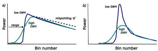
Figure 2.
Schematic of radar altimeter waveforms from (a) conventional (LRM) processing and (b) delay-Doppler processing. The increased wave height reduces the steepness of the leading edge in both cases but is also discernible in the trailing edge in delay-Doppler processing. For LRM processing, a mispointing of instrument boresight from nadir can flatten the slope of the trailing edge (black dashed line). [A more detailed exposition of the effect of wave height on waveform shape is provided in Figure 9b of [22]].
An advance in instrument design was the delay-Doppler altimeter (DDA) that recorded information on both the time delay of the echo and its Doppler shift [23]. LRM altimeters had an effective ground footprint that was a disc of order 7 km across, with the width depending upon altimeter operating parameters and wave height [7,8]. The retention and utilisation of the Doppler information (via SAR-like processing) enables the localisation of the received signal to a thin strip on the surface, offering finer along-track resolution. The DDA waveform shown in Figure 2b has the power concentrated in a narrower range of waveform bins, with wave height affecting the shape of both the leading and trailing edges. This requires a different retracking algorithm, with SAMOSA [24] being the most commonly used. Data from these more recent instruments can also be processed to produce LRM waveforms, with MLE-4 or alternative retrackers applied. This gives consistency with the processing of the first instruments, but at the cost of losing the finer resolution available through DDA processing.
Many other LRM and DDA retrackers exist. The Sea State CCI project has evaluated the retrievals of wave height from a number of these [25]; in this paper, I aim to concentrate on the factors that affect the consistency of measurements from the most commonly available retrackers, rather than to develop new ones.
2.2. Definition of
The power in the returned radar echo, P, could be defined as the summation of the signal over a sufficient reception time. In practice, the reception window is finite in length, so instead, retracking fits an expected shape to the radar waveform, and the amplitude of that is used as an indicator of the total power. Expressed in logarithmic units, the calculation to infer (the normalised radar cross-section of the surface) is as follows:
where is the strength of the emitted pulse, A contains all the radar constants related to antenna beamwidth and radar wavelength, represents the attenuation in the receiver chain, summarises the atmospheric absorption, and the term involving height above the surface, h, gives the diminution of the signal due to spherical spreading. The attenuation term, , includes both losses in the waveguide plus deliberate fixed reductions in strength, so that the signal reaching the detector does not exceed a hard limit but is large enough that little precision is lost on digitisation.
Some of these terms are known with high precision; e.g., the altimeter’s distance from the surface is known to within a few parts in [26]. Also, the atmospheric attenuation due to water vapour and liquid water is estimated from synoptic radiometer measurements, agreeing with that from atmospheric reanalyses to within 0.01 dB [27]. Terms such as and are determined on the ground pre-launch but may subsequently change as a result of use or degradation due to long exposure to hard radiation. Consequently, most altimeters have included an internal calibration loop whereby a much attenuated version of the emitted signal is fed directly into the receiver chain. This has revealed reductions in emitted power of order 1 dB over a few years (e.g., Figure 5 of Quartly et al. [28]). These calibrations are fed into the processing chain to mitigate the reduced intensity of the emitted pulses. However, such procedures do not account for deterioration of the antenna dish, losses in any waveguide or uncertainty in the values of the attenuators used; thus, it is beneficial to have some methodology for assessing the corrected values.
2.3. Recalibration of Altimeter Values
There have been great uncertainties in the absolute calibration of , with the mean Ku-band value for Envisat being 11.1 dB, whilst that for Jason-1 was 13.9 dB, although they both operated at the same time. This relates to complexities in the actual definition, limited knowledge of the absolute power of the emitted pulse and the diminution of the signal provided by the antenna, waveguides and internal electronics. It has proven difficult to make fiducial reference measurements of sufficient accuracy, with a series of calibrations for Envisat exhibiting variability with apparent steps of up to 0.2 dB [29], which is far larger than that needed for determination of long-term trends in wind speed. There is also marked degradation in the emitted power during the many years of operation, with uncertainty about the inferred corrections.
Thus, there is a need for a robust independent means of monitoring any changes in calibration. The intention of this work is to develop a data-driven method for producing consistent values spanning multiple decades by quantifying the various factors affecting estimates.
3. Results
In the first part of the Section 3, I investigate how the choice of a retracker affects the estimates of by comparing simultaneous estimates from alternative retracking approaches. In the subsequent parts, I build on the concept of “constant reference surfaces” proposed by Quartly [19], which can be used to compare sigma0 data that do not overlap in time and space, enabling assessment of potential drift in an instrument, and also to intercompare data from different dual-frequency altimeters.
3.1. Comparison of Retrackers
Jason-3 records average LRM waveforms every 0.05 s, which are transmitted to ground receiving stations and subsequently processed using both MLE-3 and MLE-4 retrackers. For many purposes, scientists use the 1 Hz values obtained by averaging these parameters in groups of 20. Although this does reduce variability, there are still significant differences in the estimates from the two retrackers. The mean difference between the two (Figure 3c) is close to zero but varies with conditions, being ∼0.02 dB for values < 15 dB but rising to ∼0.2 dB in the very calm (and rare) conditions when exceeds 18 dB. There is, however, significant variation in the mean, with the standard deviation (s.d.) of their difference being ∼0.15 dB over most conditions but rising markedly in those extra-calm conditions. A significant part of this variability is on very short spatial scales. The exercise was repeated, with all data averaged over nine consecutive records. The scatter is reduced to about 40%, which is close to the value of expected if all the variation between MLE-3 and MLE-4 estimates was random and totally uncorrelated.
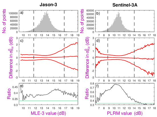
Figure 3.
Comparison of 1 Hz Ku-band values from different processing options for the same satellite. Left-hand side shows MLE-4 values compared with MLE-3 for Jason-3 altimeter; right-hand side shows comparison of delay-Doppler values against against PLRM for Sentinel-3A, using approximately 2 months of data for each. (a,b) Histograms of the reference value, with dashed lines marking the 5th and 95th percentiles. (c) Central red line shows mean difference between MLE-4 and MLE-3 estimates with outer ones showing ±2 s.d. (d) As for (c) but showing delay-Doppler relative to PLRM. (e,f) Fractional reduction of scatter upon applying a 9-point running mean. The green lines show , which is the expected value if all 1 Hz differences were totally uncorrelated. All processing used 0.1 dB wide bins.
A similar approach is applied to the MLE-4 and DDA estimates of from Sentinel-3A. [The histograms of data for Jason-3 and Sentinel-3A (Figure 3a,b) differ markedly, due to their different implementations]. There is greater variation in the mean difference of the DDA and PLRM estimates, ranging from +0.05 dB at < 8 dB to −0.05 dB for > 13 dB. The variability, indicated by the scatter of differences, is again small (s.d. is ∼0.15 dB) where the majority of data lie, but increases markedly for both very high and very low . Application of a nine-point smoother prior to comparison shows much less reduction in the s.d. (Figure 3f), indicating that there are factor(s) affecting the DDA-PLRM difference that are coherent over at least tens of kilometres.
These comparisons do not show that one estimate is better than the others, but that there are differences associated with the processing choice. In much of the subsequent analysis, I concentrate on the estimates of LRM retracking by MLE-3 or MLE-4, as that is pertinent to all instruments, and the difference between MLE-3 and MLE-4 almost disappears upon averaging many observations.
3.2. Constant Reference Surface
For many satellite sensors, useful monitoring and intercalibration may be achieved through comparison of data across regions that are constant in their properties or vary in a well-monitored way. For example, parts of the Amazon Forest are used as reference areas for microwave radiometers [30] and scatterometers [31]. For altimeters, deserts were considered almost unchanging, although the backscatter properties varied regionally due to changes in surface roughness, soil moisture and grain size [32]. Li et al. [33] identified a small section of the Taklamakan Desert in China that exhibited repeatability of measurements to within ∼0.3 dB, but the aim in this current paper is to achieve an accuracy much better than that. However, the variation in with wind speed means that no oceanic site offers this constancy, and even the global mean value cannot be considered unchanging, because the wind field varies both seasonally and interannually, so that a procedure to maintain a fixed mean value of would negate the potential to detect global climate change. Land surfaces, such as deserts or tropical rain forests, are also subject to slight seasonal and interannual variability. Instead, we focus on the constancy of the joint observations at both the Ku-band and C-band, as illustrated in Figure 4.
An increase in wind speed enhances the roughness at all scales (Figure 4b) and thus reduces the values, but not equally. Consequently, the difference in values at the Ku- and C-band has a peak, which corresponds to conditions of about 6 ms−1 (Figure 4c). Comparison of a pair of higher frequencies (shorter radar wavelengths), e.g., the Ku- and Ka-band, leads to a peak in difference at a gentler wind speed, and comparison of lower frequencies moves the peak to a higher wind speed, as shown by Figure 7b of Quartly [34].

Figure 4.
The correspondence of the values at two different radar frequencies. (a) Histogram of backscatter measurements at the C-band. (b) Simultaneous backscatter measurements at the C-band and Ku-band, with very calm conditions (low wind speeds) producing high values of and and increasing wind speeds lowering both measures. (c) Difference in values as a function of the backscatter at the C-band, with the solid red line showing the mean relationship and the dashed ones indicating ±2 s.d. in 0.1 dB wide bins. Rain, which attenuates the Ku-band signal [35], will lead to a small number of points below the mean curve [36]. [All plots are for global data from Jason-3 during cycles 33–38].
An illustration of this constancy is provided by comparing the dual-frequency backscatter statistics of two very different regions: the North Atlantic (40°N–62°N) and the Equatorial Indian Ocean (10°S–10°N). The typical wind conditions in these two regions are very different, as evidenced by a shift of ∼1.5 dB in their median values (Figure 5a) and a similar change at the Ku-band. However, the relationship between the observations at the two frequencies is very nearly the same, with the mean - curves only differing by 0.1 dB (Figure 5b), with similar amounts of scatter (Figure 5c). To enable robust monitoring of values throughout the duration of missions, and between different satellites, we now explore the various factors that contribute to this small regional difference.

Figure 5.
Constancy of the - relation. (a) Histogram of data for North Atlantic and Equatorial Indian Oceans, using Jason-3 data from cycles 33-38. The thick vertical lines mark the median values (14.45 dB and 15.95 dB, respectively). (b) Associated - curves. (c) Scatter, i.e., standard deviation of - values within each 0.1 dB wide bin. Thus, the two regions differ in their median values by 1.50 dB, but the peak of the - relationship changes by only ∼0.1 dB
3.3. Wave Height
One factor that was identified early in studies of dual-frequency sigma0 comparisons is significant wave height (SWH). The tight relationship generally observed between and is due to the prevailing winds having an almost instantaneous effect on the roughness at the scale lengths of interest. However, for the calmest wind conditions (typically <5 m s−1), the existence of large waves (swell) modulates the wind’s ability to cause roughness, as there is greater shelter in the troughs of the waves. This has an effect on the differential that is roughly proportional to wave height (Figure 6). This was first observed for TOPEX [37,38]; similar effects were noted when contrasting the and of Envisat [39]. There are also some effects associated with larger waves in high-wind conditions, but it is less clear whether these effects are actually occurring in or .
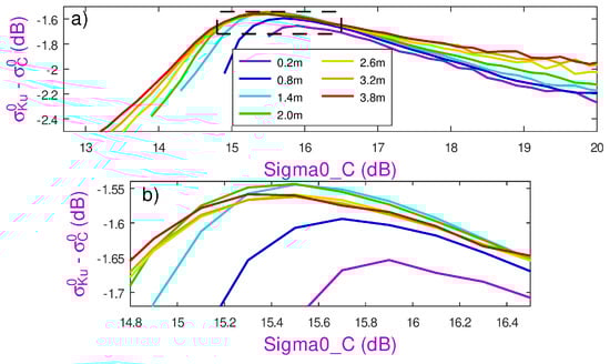
Figure 6.
Variation in the - curves with wave height. Different coloured lines represent different wave heights (±0.15 m), with the lower panel (b) being a zoom of the upper panel (a) to emphasise that there is little variation in the location of the peak for wave heights between 1.4 m and 3.2 m.
Figure 7 shows a comparison of the - curves from five different altimeters after applying a constraint to ensure the wave height ranges are the same. The instruments chosen are those that occupied the so-called 9.92-day “reference orbit” and between them span over two decades of measurements. The left-hand panel shows the different curves when the original sigma0 data from the geophysical data records (GDRs) are used, indicating a marked shift in the calibrations between TOPEX and Jason, as can also be noted from synoptic data during the TOPEX-Jason tandem phase [40]. This panel also shows some differences between the various Jason satellites. By defining a reference mean relation (shown by the black dotted line), the curves for all missions can be translated to show that the shapes of the peaks are very similar. This shift defines an instrumental correction, which will be pertinent to the particular ground processing applied, and may vary gradually with time to compensate for instrument degradation.
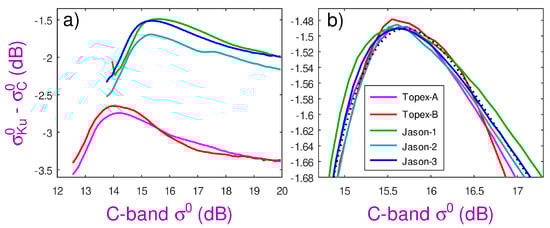
Figure 7.
Comparison of the mean - curves for 5 different altimeters. (Topex-A and Topex-B were two instruments used sequentially on the TOPEX/Poseidon satellite.) (a) The curves initially occupy very different spaces because of the different definitions used in processing, but their shapes are broadly similar. The secondary peak in the Jason-2 curve is a processing artefact, which is estimated and corrected for in the appendix. All curves were generated using data with Hs in the range 1.8–2.4 m. (b) All curves shifted to co-align, demonstrating the shape of the peak is the same (note much finer y-axis). The black dotted line provides a generic shape generated from all adjusted missions.
3.4. Sea Surface Temperature
A second factor is the sea surface temperature (SST). Vandemark et al. [41] identified that temperature had a noticeable effect on the reflectivity of sea water, with the magnitude of the effect being greatest at high frequencies (such as the Ka-band). Figure 1 of their work suggests that as SST changes from 0 °C to 30 °C, the reflectivity at the Ku-band increases by 3%, whereas that at the C-band decreases by 1%. Converting these (theoretical) values into decibels, we find an expected change in differential (Ku-band minus C-band) of 0.17 dB.
To observe these relatively small changes, I focus on the height of the peak of the - curve (i.e., maximum of -), using data corresponding to a wave height of 2.1 ± 0.3 m (to mitigate any effect of wave height). Figure 8 shows the results for four different altimeters (once they have been globally adjusted to have the same mean relationship; see Figure 7b). The curves for these four separate instruments exhibit very similar dependence upon SST, with a change from 0 °C to 30 °C corresponding to an observed raising of the peak by 0.19 dB, i.e., in close agreement with Vandemark et al. [41].
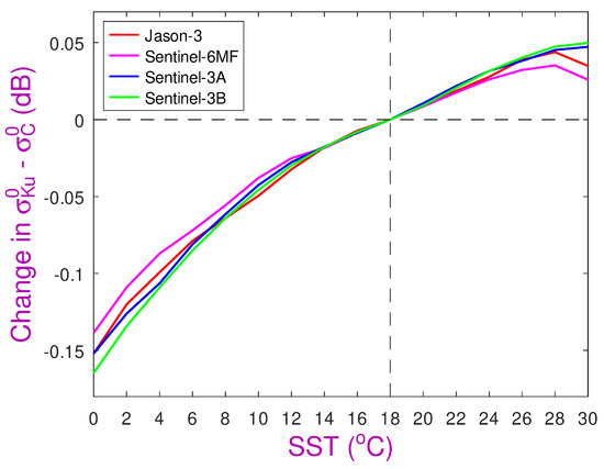
Figure 8.
Maximum of the curve of difference as a function of SST, using bins of width 2 °C. Data are shown for four independent satellites with different orbits and periods, yet the curves agree to within 0.02 dB. (All corrections have been referenced to their value at 18 °C.)
3.5. Mispointing Angle,
As stated earlier, a waveform-derived mispointing value is part of the output of the MLE-4 retracker. Most altimeter satellites have had an active attitude and orbit control system (AOCS) that maintains the correct orientation, and thus variations in the slope of the waveform trailing edge are generally small and have roughly as many negative as positive values, although designated as the square of a variable. Indeed, Challenor and Srokosz [42] identified that the MLE-4 algorithm could be ill-determined, with significant cross-talk between errors in and . Their insight was borne out initially by analysis of Jason-2 [43] but also subsequently noted for all other altimeter products using MLE-4.
Figure 9 shows the changes in the - curve with different values of . Note that due to its much broader antenna beamwidth, C-band values are only nominally affected by true platform mispointing, and thus, the simpler and computationally faster MLE-3 algorithm is usually used for the retracking of C-band waveforms. The bias in the values scales linearly with and is almost constant across all wind conditions. As this is an artefact coming out of the processing chain, the scale factor relating the change in to will depend upon the particular implementation, e.g., height of satellite and how many waveform bins are used in the inversion. For the Sentinel-3A data shown in Figure 9, a change in of 0.01° equates to a bias in of ∼0.1 dB.

Figure 9.
Variation in - curves with mispointing (specified in in the figure legend). Data are from PLRM processing of Sentinel-3A for January 2022, with the y-axis showing the mean difference between the Ku- and C-band values. The mispointing () is estimated from the waveforms, and it is the Ku-band value that is most affected by .
3.6. Radial Velocity
As the high-resolution DDA processing utilises information from the Doppler shift of the echoes to achieve its narrow footprint, there was concern that the radial component of the satellite’s velocity might affect estimates. (The satellite’s orbit is not perfectly circular, and the Earth is approximately an oblate spheroid with polar diameter 42 km less than the equatorial one, so there are well-determined changes in orbital height relative to the reference ellipsoid.) Consequently, the difference between the two Ku-band definitions of has been investigated as a function of vertical velocity (Figure 10a). At first glance, there appear to be marked changes with vertical velocity, but the change with is similar to that shown in Figure 3d, and the pattern of variation within that domain is strongly influenced by the different latitudes with which they correspond. Thus, latitudinal variations in SST and wave height contribute to the pattern observed in Figure 10a. The anomalous values for low vertical velocities are due to that region encompassing data from the Arctic, where there may be observations over sea ice that have escaped the flagging procedure. Consequently, a constraint on latitude () of is also applied.
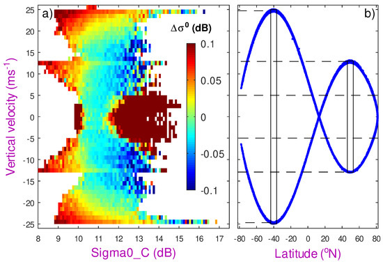
Figure 10.
Apparent effect of Sentinel-3A’s vertical velocity. (a) Difference between the estimates of from processing of Doppler waveforms and LRM waveforms, as a function of and the vertical velocity of the satellite. (b) Vertical velocity as a function of latitude for 800 orbits, showing the clear association of velocities of ±13 ms−1 with latitudes of 40°–46°N and for ±24.5 ms−1 with 42°–36°S. Lower values () may come from 5°–21°N or from the turning latitudes of the orbit ().
4. Geographical and Temporal Correlations
The strong association between vertical velocity and latitude shown in Figure 10 provides a useful illustration of the challenges in compensating for various ancillary factors: almost all have some strong variation with latitude and may also show seasonal variations. The waveform-derived mispointing, , varies rapidly on short spatial scales, whereas the true platform mispointing is usually close to zero or varies only over planetary scales. Consequently, a high-pass filter can be used to identify the amount that the mispointing affects the estimates of sigma0.
As noted earlier (Section 3.5), the waveform-derived mispointing is primarily an artefact of the retracker; however, there are environmental factors that influence it. Figure 11 shows the geographical variations of in the current release of data from Sentinel-3A. For this instrument, the mean value of is small and negative across all latitudes (Figure 11a); this may indicate a slight mismatch between the expected waveform trailing edge and that collected by this particular instrument. Note the root mean square (r.m.s.) variability (Figure 11b) is typically a factor of twenty greater than this. Poleward of 55°S and 65°N, the occasional presence of sea ice leads to much greater variability in and a decrease in the mean. Figure 11c shows that the geographical variation is not simply a function of latitude. The greatest variability is found in regions associated with the intertropical convergence zone (ITCZ) and the South Pacific convergence zone (SPCZ). This is because spatial inhomogeneities in the attenuation by rain lead to greater variability in the waveform shape. (For AltiKa, this sharp spatial variation in was used as a means for flagging for the presence of rain [44].) However, the ITCZ and SPCZ are also regions with often very low winds (high ), and so extreme values of may be associated with particular wind–wave conditions (Figure 12). In this analysis, the mean value of appears slightly heightened for high (low winds) and also especially for the highest waves for those wind conditions. This may again be due to rain, because, as well as affecting , it can broaden the leading edge of the waveform, leading to spurious high wave height estimates.
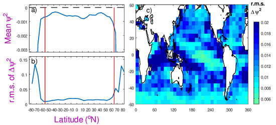
Figure 11.
Geographical variation in (in ) using PLRM data from Sentinel-3A during January 2022. (a) Latitudinal variation of mean value. (b) Latitudinal variation of variability (r.m.s. of high-pass component). (c) Map of r.m.s. variability.
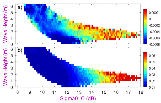
Figure 12.
Variations in in wind–wave space, with acting as a proxy for wind speed (high implies low wind speed). (a) Mean of . (b) R.m.s. variability of high-pass fluctuations.
Finally, I revisit the anomalous 59-day periodicity in noted for satellites in the TOPEX/Jason “reference orbit”. This effect has an amplitude of about 0.06 dB and is an aliasing period borne out of the satellites flying in a non-sun-synchronous orbit. Quartly [45] hypothesised that the phenomenon might be related to the percentage of time that the Jason spacecraft stayed in the shadow of the Earth, i.e., a modulation of the exposure to solar irradiation. There were also regular spacecraft re-orientation manoeuvres linked to the need to optimise the use of the solar array. Figure 13 shows an investigation of this phenomenon for 2020–2022, covering the period when the Sentinel-6MF spacecraft was launched into the reference orbit to take over from Jason-3.
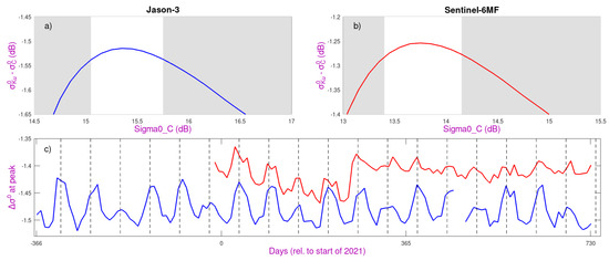
Figure 13.
Portrayal of 59-day variation in . As it is of small amplitude, it is shown as the difference () only averaged near the peak of the - curves and for . (a) For Jason-3, averaging is performed within the range of dB. (b) For Sentinel-6MF, averaging is performed within the range of dB. (c) Temporal variation in the peaks of the two - curves, with that for Jason-3 shifted up by 0.25 dB for ease of comparison. Dashed lines mark 58.77-day intervals (Sentinel-6MF only became operational towards the end of December 2020).
The - curves for the two differ in absolute position because of the calibration issues discussed earlier. (Sentinel-6MF data for this period are from the processing; a more recent change to brought them more in line with Jason-3 values.) For each altimeter, data are only considered for wave height in the range [1.8 m, 2.4 m] to minimise their effect, and averaging was performed over a narrow range at the peak of the curve. The 59-day periodicity is present for both instruments, which is interesting because the spacecraft bus for Sentinel-6MF was very different from those of the Jason satellites, instead having solar panels on two sides of a tent-like shape. However, the effect is still present, although much reduced; this suggests that it is the aliasing of a diurnal geophysical signal. Application of the SST correction from Figure 8 led to only a slight reduction. It is plausible that this residual effect relates to diurnal changes in the air–sea temperature difference, with the atmosphere having the greater diel variation.
5. Discussion
The record from altimeters is a valuable measure of the climate, but its interpretation requires understanding of the many factors that affect the quality of the data, with the aim that all records can be corrected to a consistent standard. Whilst there are internal calibration loops, an independent technique to assess any changes is essential. New retrackers and new processing techniques (such as DDA) can offer improvements to the altimetric record, but, to enable reliable trend analysis, measurements need to be unbiased with respect to previous methods.
Figure 3 shows that different techniques applied to the same data led to r.m.s. discrepancies of ∼0.15 dB for 1 Hz data. For many applications, “super observations” corresponding to averages over 50 or more kilometres are used. Much of the discrepancy between different methods will be smoothed out, but the fact that the bias is non-zero and varies slightly with means that long-term analysis is best achieved with a consistent estimate of across all missions. The various tandem missions have afforded a good intercalibration between altimeters operating in the “reference orbit” but cannot link the sequential TOPEX-A and TOPEX-B instruments or allow for aspects of instrument drift that are not fully monitored. The application of the dual-frequency reference technique does provide this.
Central to this method is that there is a tight mean relationship between nadir backscatter at the Ku- and C-band. This should be a physical property that changes minimally in time and space. Figure 5 shows that the mean curves differ by only 0.1 dB between two very disparate regions for which the median measure differed by 1.5 dB. However, to link non-overlapping missions to a better precision than that requires an understanding of the physical causes of the observed difference.
Wave height was shown to have an effect on the interplay between and [37,38], but Figure 6b shows that for a moderate range of wave heights, the effect at the peak of the - curve was minor. The other strong effect was caused by SST, with the observed changes shown in Figure 8 for altimeters, agreeing well with that predicted from studies on the emissivity of sea water. (Although rain can have a marked effect on , it typically affects less than 5% of data, and its effect can be mitigated by use of robust statistical measures that discard outliers.) By focusing on wave heights in the range 1.8–2.4 m and applying an SST correction derived from the global studies, the mean - curves for the North Atlantic and Equatorial Indian Ocean agreed to within 0.01 dB. Tran et al. [46] noted that adjustments to to account for SST will ultimately feed through into changes in the sea state bias correction [47,48] used to calculate accurate sea level from altimetry.
Figure 7 shows that the mean - relationships for a number of dual-frequency altimeters do have the same curve shape, albeit shifted according to the calibrations applied in their respective ground processing chains. (Note the curve for Jason-2 shows an anomalous secondary peak; the appendix of this paper shows that this was traced to an error in the processing chain, and that rectification removes this spurious feature).
The processing for the latest satellite to occupy the “reference orbit”, Sentinel-6MF, has undergone a number of evolutions. The last change, from “f08” to “f09”, included an additional bias to of 0.91 dB. This adjustment is independently validated by the dual-frequency reference technique. Figure 14 shows that the necessary translation to co-align the two - curves is 0.91 dB (to within 0.01 dB). This equates to an adjustment of both and by 0.91 dB and was evaluated through comparison of periods two months apart. (A total reprocessing of the Sentinel-6MF data, “g01”, is expected in late 2025.)

Figure 14.
Comparison of curves for Sentinel-6MF from two different processing versions. The blue curve is from cycles 107–118 processed with f08, and the green curve is for cycles 123–134 processed with f09. The dashed red line shows the blue curve shifted horizontally by 0.91 dB.
An improved multi-satellite sigma0 dataset should not only enable a more consistent altimetric wind speed record, but also for other parameters that depend on sigma0, such as wave period [49,50] and air–sea gas transfer velocities [51,52].
The TOPEX/Jason repeat cycle of 9.92 days contains typically 380,000 marine observations, the majority of which lie close to the peak of the - curve, thus allowing a good assessment of the calibration every cycle. The TOPEX-A instrument was known to suffer from degradation in space, with changes in all its derived parameters, especially wave height (see Figure 2 of Queffeulou [53]). Figure 15 shows the wind speed statistics for a period of 5 years spanning the transition in operating instruments. Whilst there will be changes in the wind climate with time, a step change coincident with the change in instruments is suspicious. Using the dual-frequency technique, I obtained relative offsets for each cycle and then applied the same wind speed algorithm as on the original TOPEX GDRs. The result is a smoother transition, not just in the median but also the range of conditions noted by the 25th and 75th percentiles. This is consistent with the meteorological reanalysis interpolated to the TOPEX observation points.
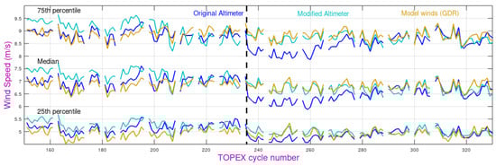
Figure 15.
Statistics of wind speed during each 9.92-day cycle of TOPEX data from cycle 151 (October 1996) to 330 (September 2001), noting the change in operating instrument from TOPEX-A to TOPEX-B after cycle 235. The dark blue curves show the altimeter-derived wind speed on the GDRs using the distributed values, whilst the light blue shows the values for the same algorithm after correction for derived drift. The orange lines show the values from the ECMWF reanalysis at the same locations (The 25th, 50th and 75th percentiles are calculated over the region 55°S to 60°N to avoid sea ice, and there are gaps in the series when the Poseidon single-frequency altimeter was operating instead).
Other than wind speed, the key factors affecting sigma0 are wave height and SST. To produce a long-term altimetric wind speed dataset independent from other satellite sensors requires adjustment for these two factors (plus the AGC for Jason-2), so that trends derived from altimeter winds will not be biased by long-term changes in SST or waves. Other factors, such as waveform-derived mispointing and radial velocity, appear to be either minor or an artefact of the processing chain or a geographical correlation with one of the dominant terms. These can be avoided by consistent use of a basic retracker, such as MLE-3.
6. Conclusions
There are presently large offsets between the values from different altimeter missions, as well as possible drifts in performance despite internal monitoring. To achieve long-term consistent sigma0 records from altimeters requires great care in adjusting the offsets between missions and in correcting for any drift. Simple biases are readily applied between missions, but that could hide any long-term changes. Although individual papers have shown to vary with wave height as well as wind speed, or looked at differences between alternative retracking solutions, this paper brings together investigation of a large number of effects in a consistent manner, identifying which factors have the greater effect and how geographic correlations can give the appearance of other dependencies. After mitigating the effects of the two dominant terms (wave height and SST), the near-constancy of the - relationship at the Ku- and C-band can be used to assess step changes or drifts in values from a dual-frequency altimeter, and to determine relative offsets between missions that did not overlap in time. This novel method for enforcing a consistency in observations spanning multiple missions is demonstrated for both changes during a mission lifetime and for assessing inter-mission biases. A fully consistent multi-decadal dataset could be used for climatological studies of wind speed, wave period and occurrence of air–sea transfer of climatologically important gases.
7. Appendix: Determining Appropriate AGC Corrections for Jason-2
When standard - curves were calculated for Jason-2, they were found not to have the simple shape, with one smooth peak, noted for the other dual-frequency altimeters. Instead, the resultant mean relationship had a secondary peak that, over the initial 8 years of the mission, could be seen to migrate towards higher values. It was eventually surmised that there might be a problem with the AGC corrections implemented in the Jason-2 processing. The automatic gain control (AGC) is a system of attenuators that are switched in within the receiver chain in order to keep the amplitude of the received waveform within acceptable bounds. In short, it aims to provide the best dynamic resolution of the waveforms by keeping the waveform amplitude large without it saturating (reaching a hard limit in the power summation at any of the waveform bins). Over the vast majority of ocean returns, the returned echoes conform to the Brown-like shape [1,2], and thus, the AGC works well and prevents waveform saturation and loss of information.
The formula for calculating is given by Equation (1), with separate estimates every 0.05 s (for Jason-2). In that time, the satellite and its nadir footprint only move 330 m, whilst the footprint itself represents the return over a disc 7 km in diameter [7,8]. Consequently, over most of the ocean, there will be minimal change in the area-averaged backscatter values. However, the AGC has a fixed set of finite values and switches between these as needed. A higher AGC setting should result in a lower received power, P.
The approach developed here examines cases where the AGC is flipping back and forth between two neighbouring values (so there is negligible change in the true ground conditions). If there is an actual change in the AGC setting of , but the ground processing assumes the nominal value of , then the erroneous compensation will result in the calculated changing by (see Figure 16). This can be determined by averaging over thousands of transitions and for different cycles (periods of data). [Note this method only finds the difference between two given AGC settings; it does not provide absolute values for any setting. It has previously been used for Poseidon [54] and for examining the biases associated with changes in the gate index in the original TOPEX processing [55]].

Figure 16.
Schematic showing estimation of error in AGC corrections. For a given AGC setting, instances are noted when the altimeter temporarily changes to a higher setting and returns (left-hand column) or when it is at the higher setting and temporarily drops back to the ith AGC setting and returns. The nominal difference between the two settings is agc, whilst the actual difference is agc + agc. If there is no change in the underlying surface properties, there will be an associated change in the sum of powers in the waveform bins, (or other estimate of amplitude of waveform), by agc + agc. However, the calculated only uses the nominal change in the AGC setting, so there will be an observed change in agc. Evaluation over thousands of instances enables a reliable estimate of the error in AGC corrections, agc.
Over the non-coastal ice-free ocean, the vast majority of Ku-band observations are covered by 10 AGC settings (and a different set of 10 for C-band). In the analysis shown in Figure 17, the mean associated with each of these nine changes is determined for four cycles spanning the Jason-2 mission. The two columns for each cycle represent the independent results for a temporary “up transition” (left-hand side of Figure 16) and a temporary “down transition”. There is a very high consistency between the results for different cycles, showing that there is no appreciable degradation in the attenuators’ performance. With steps between nominal AGC values being of order 1 dB, the errors can be seen to be of order 5%; however, the cumulative total of the errors over those nine transitions is ~0.2 dB (for both Ku-band and C-band).
A correction is then readily implemented using a bit-wise linear interpolation between these observed cumulative errors (Figure 18). This correction is applied to five Jason-2 cycles a year apart, with the chosen cycles being different from those used in determining the AGC errors. The change in the resultant - curves is profound (Figure 19), with the secondary peak being smoothly eradicated in all cases (although corresponding to different values) and the shape of the - curves matching those of other dual-frequency altimeters.

Figure 17.
Evaluated changes associated with the main AGC settings for Jason-2 at the Ku-band and C-band. Analysis was performed for 4 cycles spanning Jason 2’s lifetime, with separate estimations for the two scenarios depicted in Figure 16. [Units are millibels, i.e., hundredths of a decibel. Note that even columns have had a sign reversal applied to match the odd columns].

Figure 18.
Corrections to be applied to GDR values as a function of AGC setting. (a) Ku-band. (b) C-band. Adjustments were evaluated for discrete settings shown by blue dots but are implemented for the whole range of AGC values (shown by black lines).

Figure 19.
Plot of - curves for 5 Jason-2 cycles approximately a year apart. Left-hand plot shows curves using original data from GDRs; right-hand one shows curves after correction for AGC errors.
Funding
This research was funded by the European Space Agency (ESA) through the Sea State CCI (Contract No. LS275614-4000123651). The views expressed herein can in no way be taken to reflect the official opinion of the European Space Agency.
Data Availability Statement
All altimeter data are available from the sources detailed in Table 1.
Acknowledgments
This work made use of the generally free access to altimeter data provided by ESA, NASA, CNES and EUMETSAT. One set of SST data was from daily fields of microwave-derived SST from AMSR-E [56] and AMSR2 [57], which were produced by Remote Sensing Systems and were sponsored by the NASA AMSR-E Science Team and the NASA Earth Science MEaSUREs Program. These data are available at www.remss.com. Further SST data came from the ECMWF Reanalysis, and I am grateful to Jean-Francois Piolle for extracting all the relevant locations. I also acknowledge the prompt response concerning EUMETSAT processing provided by Salvatore Dinardo, Cristina Martin-Puig and Bruno Lucas.
Conflicts of Interest
The author declares no conflicts of interest.
References
- Brown, G. The average impulse response of a rough surface and its applications. IEEE Trans. Antennas Propag. 1977, 25, 67–74. [Google Scholar] [CrossRef]
- Hayne, G. Radar altimeter mean return waveforms from near-normal-incidence ocean surface scattering. IEEE Trans. Antennas Propag. 1980, 28, 687–692. [Google Scholar] [CrossRef]
- Ridley, J.K.; Bamber, J.L. Antarctic field measurements of radar backscatter from snow and comparison with ERS-1 altimeter data. J. Electromagn. Waves Appl. 1995, 9, 355–371. [Google Scholar] [CrossRef]
- Arthern, R.J.; Wingham, D.J.; Ridout, A.L. Controls on ERS altimeter measurements over ice sheets: Footprint-scale topography, backscatter fluctuations, and the dependence of microwave penetration depth on satellite orientation. J. Geophys. Res. 2001, 106, 33471–33484. [Google Scholar] [CrossRef]
- Scott, J.B.T.; Nienow, P.; Mair, D.; Parry, V.; Morris, E.; Wingham, D.J. Importance of seasonal and annual layers in controlling backscatter to radar altimeters across the percolation zone of an ice sheet. Geophys. Res. Lett. 2006, 33, L24502. [Google Scholar] [CrossRef]
- Quartly, G.D.; Rinne, E.; Passaro, M.; Andersen, O.B.; Dinardo, S.; Fleury, S.; Guillot, A.; Hendricks, S.; Kurekin, A.A.; Müller, F.L.; et al. Retrieving sea level and freeboard in the Arctic: A review of current radar altimetry methodologies and future perspectives. Remote Sens. 2019, 11, 881. [Google Scholar] [CrossRef]
- Chelton, D.B.; Walsh, E.J.; MacArthur, J.L. Pulse compression and sea level tracking in satellite altimetry. J. Atmos. Ocean. Technol. 1989, 6, 407–438. [Google Scholar] [CrossRef]
- Quartly, G.D. Determination of oceanic rain rate and rain cell structure from altimeter waveform data. Part I: Theory. J. Atmos. Ocean. Technol. 1998, 15, 1361–1378. [Google Scholar] [CrossRef]
- Gomez-Enri, J.; Vignudelli, S.; Quartly, G.D.; Gommenginger, C.P.; Cipollini, P.; Challenor, P.G.; Benveniste, J. Modeling Envisat RA-2 waveforms in the coastal zone: Case study of calm water contamination. IEEE Geosci. Remote Sens. Lett. 2010, 7, 474–478. [Google Scholar] [CrossRef]
- Gommenginger, C.; Thibaut, P.; Fenoglio-Marc, L.; Quartly, G.; Deng, X.; Gómez-Enri, J.; Challenor, P.; Gao, Y. Retracking Altimeter Waveforms Near the Coasts. In Coastal Altimetry; Vignudelli, S., Kostianoy, A.G., Cipollini, P., Benveniste, J., Eds.; Springer: Berlin/Heidelberg, Germany, 2011; pp. 61–101. [Google Scholar] [CrossRef]
- Chelton, D.B.; McCabe, P.J. A review of satellite altimeter measurement of sea surface wind speed: With a proposed new algorithm. J. Geophys. Res. 1985, 90, 4707–4720. [Google Scholar] [CrossRef]
- Witter, D.L.; Chelton, D.B. A Geosat altimeter wind speed algorithm and a method for altimeter wind speed algorithm development. J. Geophys. Res. 1991, 96, 8853–8860. [Google Scholar] [CrossRef]
- Abdalla, S. Ku-Band radar altimeter surface wind speed algorithm. Mar. Geod. 2012, 35, 276–298. [Google Scholar] [CrossRef]
- Young, I.R.; Zieger, S.; Babanin, A.V. Global trends in wind speed and wave height. Science 2011, 332, 451–455. [Google Scholar] [CrossRef] [PubMed]
- Young, I.; Donelan, M. On the determination of global ocean wind and wave climate from satellite observations. Remote Sens. Environ. 2018, 215, 228–241. [Google Scholar] [CrossRef]
- Gourrion, J.; Vandemark, D.; Bailey, S.; Chapron, B.; Gommenginger, G.P.; Challenor, P.G.; Srokosz, M.A. A two-parameter wind speed algorithm for Ku-Band altimeters. J. Atmos. Ocean. Technol. 2002, 19, 2030–2048. [Google Scholar] [CrossRef]
- WMO. The 2022 GCOS ECVs Requirements. Document GCOS-245. Available online: https://meetings.wmo.int/INFCOM-2/InformationDocuments/INFCOM-2-INF06-1(11-2)-2022-GCOS-ECVS-REQUIREMENTS_en.pdf (accessed on 17 April 2025).
- Dodet, G.; Piolle, J.F.; Quilfen, Y.; Abdalla, S.; Accensi, M.; Ardhuin, F.; Ash, E.; Bidlot, J.R.; Gommenginger, C.; Marechal, G.; et al. The Sea State CCI dataset v1: Towards a sea state Climate Data Record based on satellite observations. Earth Syst. Sci. Data Discuss. 2020, 2020, 1929–1951. [Google Scholar] [CrossRef]
- Quartly, G.D. Monitoring and cross-calibration of altimeter σ0 through dual-frequency backscatter measurements. J. Atmos. Ocean. Technol. 2000, 17, 1252–1258. [Google Scholar] [CrossRef]
- Amarouche, L.; Thibaut, P.; Zanife, Z.O.; Dumont, J.P.; Vincent, P.; Steunou, N. Improving the Jason-1 ground retracking to better account for attitude effects. Mar. Geod. 2004, 27, 171–197. [Google Scholar] [CrossRef]
- Tourain, C.; Piras, F.; Ollivier, A.; Hauser, D.; Poisson, J.C.; Boy, F.; Thibaut, P.; Hermozo, L.; Tison, C. Benefits of the adaptive algorithm for retracking altimeter nadir echoes: Results from simulations and CFOSAT/SWIM observations. IEEE Trans. Geosci. Remote Sens. 2021, 59, 9927–9940. [Google Scholar] [CrossRef]
- Ardhuin, F.; Stopa, J.E.; Chapron, B.; Collard, F.; Husson, R.; Jensen, R.E.; Johannessen, J.; Mouche, A.; Passaro, M.; Quartly, G.D.; et al. Observing sea states. Front. Mar. Sci. 2019, 6, 124. [Google Scholar] [CrossRef]
- Raney, R.K. The delay/Doppler radar altimeter. IEEE Trans. Geosci. Remote Sens. 1998, 36, 1578–1588. [Google Scholar] [CrossRef]
- Ray, C.; Martin-Puig, C.; Clarizia, M.P.; Ruffini, G.; Dinardo, S.; Gommenginger, C.; Benveniste, J. SAR altimeter backscattered waveform model. IEEE Trans. Geosci. Remote Sens. 2015, 53, 911–919. [Google Scholar] [CrossRef]
- Schlembach, F.; Passaro, M.; Quartly, G.D.; Kurekin, A.; Nencioli, F.; Dodet, G.; Piollé, J.F.; Ardhuin, F.; Bidlot, J.; Schwatke, C.; et al. Round Robin Assessment of Radar Altimeter Low Resolution Mode and Delay-Doppler Retracking Algorithms for Significant Wave Height. Remote Sens. 2020, 12, 1254, Erratum in Remote Sens. 2021, 13, 1182. [Google Scholar] [CrossRef]
- Lemoine, F.G.; Zelensky, N.P.; Chinn, D.S.; Pavlis, D.E.; Rowlands, D.D.; Beckley, B.D.; Luthcke, S.B.; Willis, P.; Ziebart, M.; Sibthorpe, A.; et al. Towards development of a consistent orbit series for TOPEX, Jason-1, and Jason-2. Adv. Space Res. 2010, 46, 1513–1540. [Google Scholar] [CrossRef]
- ESA. Sentinel Online—Data Product Quality Reports. Sentinel-3 MWR Cyclic Performance Report. Available online: https://sentiwiki.copernicus.eu/web/document-library#DocumentLibrary-SRALLibrary-S3-Performance-DQR-SRAL (accessed on 11 February 2025).
- Quartly, G.D.; Nencioli, F.; Raynal, M.; Bonnefond, P.; Garcia, P.N.; Garcia-Mondéjar, A.; lores de la Cruz, A.; Crétaux, J.F.; Taburet, N.; Frery, M.L.; et al. The roles of the S3MPC: Monitoring, validation and evolution of Sentinel-3 altimetry observations. Remote Sens. 2020, 12, 1763. [Google Scholar] [CrossRef]
- Pierdicca, N.; Bignami, C.; Roca, M.; Féménias, P.; Fascetti, M.; Mazzetta, M.; Loddo, C.; Martini, A.; Pinori, S. Transponder calibration of the Envisat RA-2 altimeter Ku band sigma naught. Adv. Space Res. 2013, 51, 1478–1491. [Google Scholar] [CrossRef]
- Brown, S. Maintaining the long-term calibration of the Jason-2/OSTM Advanced Microwave Radiometer through intersatellite calibration. IEEE Trans. Geosci. Remote Sens. 2013, 51, 1531–1543. [Google Scholar] [CrossRef]
- Peng, H.; Mu, B.; Lin, M.; Zhou, W. HY-2A satellite calibration and validation approach and results. In Proceedings of the IEEE Geoscience and Remote Sensing Symposium, Quebec City, QC, Canada, 13–18 July 2014; pp. 4528–4531. [Google Scholar] [CrossRef]
- Ridley, J.; Strawbridge, F.; Card, R.; Phillips, H. Radar backscatter characteristics of a desert surface. Remote Sens. Environ. 1996, 57, 63–78. [Google Scholar] [CrossRef]
- Li, M.; Xu, X.-Y.; Jiang, M.; Yan, X. Research on the backscattering characteristics of HY-2C satellite radar altimeter over desert surface. IEEE Geosci. Remote Sens. Lett. 2025, 22, 3506705. [Google Scholar] [CrossRef]
- Quartly, G.D. Metocean comparisons of Jason-2 and AltiKa—A method to develop a new wind speed algorithm. Mar. Geod. 2015, 38, 437–448. [Google Scholar] [CrossRef]
- Guymer, T.H.; Quartly, G.D.; Srokosz, M.A. The effects of rain on ERS-1 radar altimeter data. J. Atmos. Ocean. Technol. 1995, 12, 1229–1247. [Google Scholar] [CrossRef]
- Quartly, G.D.; Guymer, T.H.; Srokosz, M.A. The effects of rain on Topex radar altimeter data. J. Atmos. Ocean. Technol. 1996, 13, 1209–1229. [Google Scholar] [CrossRef]
- Elfouhaily, T.; Vandemark, D.; Gourrion, J.; Chapron, B. Estimation of wind stress using dual-frequency TOPEX data. J. Geophys. Res. Ocean. 1998, 103, 25101–25108. [Google Scholar] [CrossRef]
- Quartly, G.D.; Srokosz, M.A.; Guymer, T.H. Global precipitation statistics from dual-frequency TOPEX altimetry. J. Geophys. Res. Atmos. 1999, 104, 31489–31516. [Google Scholar] [CrossRef]
- Tournadre, J.; Quartly, G.D. Validation of Envisat RA2 Rain Flag; Technical Report; Ifremer: Brest, France, 2004. [Google Scholar]
- Quartly, G.D. Sea state and rain: A second take on dual-frequency altimetry. Mar. Geod. 2004, 27, 133–152. [Google Scholar] [CrossRef]
- Vandemark, D.; Chapron, B.; Feng, H.; Mouche, A. Sea surface reflectivity variation with ocean temperature at Ka-band observed using near-nadir satellite radar data. IEEE Geosci. Remote Sens. Lett. 2016, 13, 510–514. [Google Scholar] [CrossRef]
- Challenor, P.G.; Srokosz, M.A. The extraction of geophysical parameters from radar altimeter returns from a non-linear sea surface. In Mathematics in Remote Sensing; Brooks, S.R., Ed.; Clarendon Press: Oxford, UK, 1989; pp. 257–268. [Google Scholar]
- Quartly, G.D. Optimizing σ0 information from the Jason-2 altimeter. IEEE Geosci. Remote Sens. Lett. 2009, 6, 398–402. [Google Scholar] [CrossRef]
- Tournadre, J.; Lambin-Artru, J.; Steunou, N. Cloud and rain effects on AltiKa/SARAL Ka-band radar altimeter—Part II: Definition of a rain/cloud flag. IEEE Trans. Geosci. Remote Sens. 2009, 47, 1818–1826. [Google Scholar] [CrossRef]
- Quartly, G.D. Jason-1/Jason-2 metocean comparisons and monitoring. Mar. Geod. 2010, 33, 256–271. [Google Scholar] [CrossRef]
- Tran, N.; Vandemark, D.; Bignalet-Cazalet, F.; Dibarboure, G. Quantifying multifrequency ocean altimeter wind speed error due to sea surface temperature and resulting impacts on satellite sea level measurements. Remote Sens. 2023, 15, 3235. [Google Scholar] [CrossRef]
- Labroue, S.; Gaspar, P.; Dorandeu, J.; Zanife, O.; Mertz, F.; Vincent, P.; Choquet, D. Nonparametric estimates of the sea state bias for the Jason-1 radar altimeter. Mar. Geod. 2004, 27, 453–481. [Google Scholar] [CrossRef]
- Tran, N.; Vandemark, D.; Labroue, S.; Feng, H.; Chapron, B.; Tolman, H.L.; Lambin, J.; Picot, N. Sea state bias in altimeter sea level estimates determined by combining wave model and satellite data. J. Geophys. Res. 2010, 115, C03020. [Google Scholar] [CrossRef]
- Mackay, E.B.L.; Retzler, C.H.; Challenor, P.G.; Gommenginger, C.P. A parametric model for ocean wave period from Ku band altimeter data. J. Geophys. Res. 2008, 113, C03029. [Google Scholar] [CrossRef]
- Zhao, D.; Li, S.; Song, C. The comparison of altimeter retrieval algorithms of the wind speed and the wave period. Acta Oceanol. Sin. 2012, 31, 1–9. [Google Scholar] [CrossRef]
- Frew, N.M.; Glover, D.M.; Bock, E.J.; McCue, S.J. A new approach to estimation of global air-sea gas transfer velocity fields using dual-frequency altimeter backscatter. J. Geophys. Res. 2007, 112, C11003. [Google Scholar] [CrossRef]
- Glover, D.M.; Frew, N.M.; McCue, S.J. Air–sea gas transfer velocity estimates from the Jason-1 and TOPEX altimeters: Prospects for a long-term global time series. J. Mar. Syst. 2007, 66, 173–181. [Google Scholar] [CrossRef]
- Queffeulou, P. Long-term validation of wave height measurements from altimeters. Mar. Geod. 2004, 27, 495–510. [Google Scholar] [CrossRef]
- Quartly, G.D.; Srokosz, M.A.; McMillan, A.C. Analyzing altimeter artifacts: Statistical properties of ocean waveforms. J. Atmos. Ocean. Technol. 2001, 18, 2074–2091. [Google Scholar] [CrossRef]
- Quartly, G.D. The gate dependence of geophysical retrievals from the TOPEX altimeter. J. Atmos. Ocean. Technol. 2000, 17, 1247–1251. [Google Scholar] [CrossRef]
- Wentz, F.; Meissner, T.; Gentemann, C.; Brenner, M. RSS AQUA AMSR-E Daily Environmental Suite on 0.25 Deg Grid. Version 7. Available online: https://www.remss.com/DOI/RSS-bm.html (accessed on 29 August 2025).
- Wentz, F.; Meissner, T.; Gentemann, C.; Hilburn, K.; Scott, J. RSS GCOM-W1 AMSR2 Daily Environmental Suite on 0.25 Deg Grid. Version 8.2. Available online: https://www.remss.com/DOI/RSS-bq.html (accessed on 29 August 2025).
Disclaimer/Publisher’s Note: The statements, opinions and data contained in all publications are solely those of the individual author(s) and contributor(s) and not of MDPI and/or the editor(s). MDPI and/or the editor(s) disclaim responsibility for any injury to people or property resulting from any ideas, methods, instructions or products referred to in the content. |
© 2025 by the author. Licensee MDPI, Basel, Switzerland. This article is an open access article distributed under the terms and conditions of the Creative Commons Attribution (CC BY) license (https://creativecommons.org/licenses/by/4.0/).