Highlights
What are the main findings?
- Our newly developed indices, ARSEI and CoRSEI, enhance ecological monitoring in arid regions, with CoRSEI integrating desert and non-desert systems.
- ARSEI is sensitive to vegetation and precipitation in deserts, while CoRSEI captures spatial heterogeneity, long-term trends, and desert–non-desert transitions.
What is the implication of the main finding?
- These indices support spatially differentiated, driver-sensitive assessments, aiding targeted ecosystem management and restoration in arid landscapes.
Abstract
Monitoring ecosystem dynamics in arid regions requires robust indicators that can capture spatial heterogeneity and diverse ecological drivers. In this study, we introduce and evaluate two novel ecological indices: the Arid-region Remote Sensing Ecological Index (ARSEI), specifically designed for desert environments, and the Composite Remote Sensing Ecological Index (CoRSEI), which integrates both desert and non-desert systems. These indices are compared with the traditional Remote Sensing Ecological Index (RSEI) in the Tarim River Basin from 2000 to 2023. Principal component analysis (PCA) revealed that RSEI maintained the highest structural compactness (average PCA1 = 87.49%). In contrast, ARSEI (average PCA1 = 78.62%) enhanced sensitivity to albedo and vegetation (NDVI) in arid environments. Spearman correlation analysis further demonstrated that ARSEI was more strongly correlated with NDVI (ρ = 0.49) and precipitation (ρ = 0.62) than RSEI, confirming its improved responsiveness under water-limited conditions. CoRSEI exhibited higher internal consistency and spatial adaptability (mean values ranging from 0.45 to 0.56), with slight ecological improvements observed between 2000 and 2023. Ecological drivers varied across habitat types. In desert areas, evapotranspiration, precipitation, and soil moisture were the main determinants of ecological status, showing high coupling and synchrony. In non-desert regions, soil moisture and precipitation remained dominant, but vegetation indices and disturbance factors (e.g., fire density) exerted stronger long-term influences. Partial dependence analyses further confirmed nonlinear, region-specific responses, such as the threshold effects of precipitation on vegetation growth. Overall, our findings highlight the importance of differentiated ecological modeling. ARSEI enhances sensitivity in desert ecosystems, whereas CoRSEI captures landscape-scale variability across desert and non-desert regions. Both indices contribute to more accurate long-term ecological assessments in hyper-arid environments.
1. Introduction
Under the accelerating impacts of global climate change and intensified anthropogenic disturbances, arid and semi-arid regions are experiencing rapidly expanding ecological challenges, particularly in ecologically fragile areas such as Central Asia, North Africa, and northern China. These regions exhibit low ecosystem stability and high sensitivity to external disturbances [1], leading to prominent issues such as habitat degradation, biodiversity loss, and declines in ecosystem service functions [2,3]. A comprehensive understanding of the spatiotemporal dynamics of habitat quality and its ecological consequences in arid zones is therefore essential. Such understanding can inform regional land management and conservation strategies, and support broader goals, including sustainable development and the achievement of global land degradation neutrality targets [4,5].
Traditional assessments using indices like the Normalized Difference Vegetation Index (NDVI) or Land Surface Temperature (LST) were limited, prompting the development of integrated approaches for more holistic ecological evaluation. Advances in remote sensing and geospatial technologies have further enabled the application of landscape pattern indices, land-use transition matrices, and particularly the Remote Sensing Ecological Index (RSEI) as key tools for analyzing spatiotemporal ecological changes [6,7,8]. The Remote Sensing Ecological Index (RSEI) integrates four indicators—NDVI, Wetness (WET), LST, and the Normalized Difference Built-up and Soil Index (NDBSI)—into a composite index. It uses principal component analysis (PCA) to reduce dimensionality and fuse data, effectively reflecting overall ecosystem health [9,10]. RSEI’s high automation, broad spatial applicability, and easy data access have enabled its widespread use in monitoring ecological dynamics under urban expansion, land degradation, and ecosystem restoration [11,12,13]. Due to varying research objectives across different regions, the RSEI exhibits limited adaptability to local ecological environments, shows insufficient sensitivity to ecological changes in some areas, and its assessment results can also be influenced by seasonal variations and spatial resolution [14,15]. As a result, modified versions have been developed, for example, by refining dryness indices in urban areas [16] or incorporating salinity and land degradation indicators in arid zones [17], demonstrating flexibility and potential for methodological refinement.
Nevertheless, some limitations remain in specific environments. In particular, NDBSI—an essential component of RSEI used to identify bare soil and built-up areas—faces challenges in desert landscapes. The high reflectance similarity between sand dunes and bare soil often causes misclassification and reduces evaluation accuracy [13,18,19]. To overcome this issue, this study proposes the Arid-zone Remote Sensing Ecological Index (ARSEI), which replaces NDBSI with surface albedo. Surface albedo, a key parameter in surface energy balance, effectively captures radiative characteristics and vegetation cover, particularly in distinguishing sandy surfaces from sparsely vegetated areas [20]. MODIS albedo products have proven capable of differentiating soil conditions in arid environments, such as separating sandy soils from saline–alkaline soils [21,22]. Consequently, ARSEI provides enhanced robustness and adaptability for assessing ecosystem health in arid and semi-arid landscapes.
In parallel, the integration of hydrometeorological indicators into ecological quality assessments has gained increasing attention, especially in arid ecosystems [23,24]. The Standardized Precipitation Evapotranspiration Index (SPEI6), for example, has been used in West Asia to investigate the relationship between water deficits and ecosystem carbon-water fluxes, showing that water stress significantly impairs ecosystem function and is further worsened by extreme events such as wildfires [25]. In oasis–desert transition zones, excessive evapotranspiration coupled with limited groundwater recharge exacerbates drought vulnerability [26]. Although extreme precipitation events may temporarily boost soil moisture, their ecological benefits are usually short-lived under hot and arid conditions [27]. Accordingly, this study also explores the responses and influences of multiple environmental drivers on RSEI in arid ecosystems.
Importantly, the surface characteristics of desert and non-desert areas differ markedly, which inherently affects ecological quality assessments. Applying uniform evaluation standards across these heterogeneous landscapes can obscure critical ecological disparities: desert areas with restoration potential may be underestimated, while ecologically vulnerable non-desert zones might be overlooked in degradation risk assessments [28,29]. To address this, we propose a Composite Remote Sensing Ecological Index (CoRSEI) tailored to the Tarim Basin, using a zonal modeling approach that accounts for the basin’s geographical heterogeneity. The desert zone is evaluated with the improved ARSEI incorporating surface albedo, while the non-desert zone employs the traditional RSEI framework. A dimension-consistent transformation (+1 shift) is applied to harmonize the indices and ensure comparability. The primary objectives of this study are to: (1) develop an optimized RSEI for desert areas by integrating surface albedo to form ARSEI; (2) construct a zonally adaptive CoRSEI to assess ecological quality in both desert and non-desert regions of the Tarim River Basin and reveal spatial ecological patterns; and (3) use multivariate statistical analyses and machine learning interpretability methods to investigate region-specific environmental drivers and their influence mechanisms. This framework addresses environmental heterogeneity in arid-zone ecological assessments and provides theoretical and technical support for targeted conservation and management in ecologically vulnerable regions.
2. Materials and Methods
2.1. Study Area
The Tarim River Basin (TRB), located in the Xinjiang Uyghur Autonomous Region of northwestern China (75–93°E, 35–43°N) (Figure 1), encompasses the approximately 1320 km long Tarim River. The basin is surrounded by major mountain ranges, including the Tianshan, Kunlun, and Pamir Mountains, and exhibits typical basin landforms. The TRB has a temperate continental desert climate, with arid conditions and low annual precipitation averaging below 50 mm, and some areas receiving less than 20 mm per year. Temperature varies greatly both annually and daily, with summer maxima exceeding 40 °C and winter minima below −20 °C. Evaporation far exceeds precipitation, ranging from 2000 to 3000 mm per year. The region also receives abundant sunshine, with annual hours typically between 2800 and 3200. Vegetation primarily consists of drought-resistant shrubs and small semi-shrubs [30], with sparse coverage in the mid and lower reaches, reflecting typical desert ecosystem characteristics. Due to water scarcity and sparse vegetation, the Tarim Basin is particularly vulnerable to the combined effects of global warming, declining rainfall, overgrazing, and over-cultivation, which accelerate land degradation and desertification [31,32]. The basin’s unique geographic location and extreme climatic conditions make it an important area for studying desert ecosystems and assessing habitat quality.
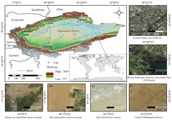
Figure 1.
Study area. The main map illustrates the elevation distribution of the Tarim River Basin and its location on the world map. The six submaps display representative land cover zones based on remote sensing imagery, including: (a) urban–farmland–desert ecotone, (b) agriculture–desert transition zone, (c) gobi desert region, (d) urban construction area, (e) lake-riparian ecosystem zone, and (f) desert landscapes.
2.2. Data Sources
2.2.1. MODIS Product Data
This study used two MODIS products as primary data sources, covering the years 2000–2023.
- (1)
- MOD09A1 (Version 6.1, NASA EOSDIS Land Processes DAAC): This product provides 500 m-resolution surface reflectance data (Bands B1–B7), including red (620–670 nm), near-infrared (841–876 nm), and shortwave infrared ranges. Cloud masking was performed using the State QA band, with bit 10 (cloud flag) and bit 11 (cloud shadow flag) applied for pixel-level filtering. To minimize transient noise, October data from each year were composited using the median to generate annual representative values, which were then clipped to the study area boundary. This dataset was primarily used to calculate the Normalized Difference Vegetation Index (NDVI), Wetness Component (WET), Normalized Difference Built-up and Soil Index (NDBSI), and Albedo.
- (2)
- MOD11A2 (Version 6.1, NASA LP DAAC): This product provides 1 km-resolution daytime land surface temperature data. The original 16-bit unsigned integer digital numbers (DN values) were converted to Celsius using the formula LST = 0.02 × DN − 273.15. Quality control was performed using bit 0 of the QC Day band to exclude cloud-contaminated pixels. To match the spatial resolution of other indices, September composite temperature data were resampled to 500 m using bilinear interpolation.
All preprocessing steps were conducted on the Google Earth Engine platform, ensuring spatiotemporal consistency across indicators at the pixel scale. Considering the characteristics of arid regions, we performed additional validation for NDVI sensitivity in low-vegetation areas and for LST accuracy over bare surfaces.
2.2.2. Environmental Drivers
The methodological workflow for processing environmental drivers used a comprehensive raster-based approach to ensure complete spatial coverage and dimensional homogeneity. First, raw environmental driver datasets were acquired from various sources (Table 1). All raster datasets were then resampled to a standardized spatial grid (0.00449° × 0.00449°, approximately 500 m × 400 m) using bilinear interpolation in Python’s rasterio library (version 1.4.3). Grid alignment was based on the study area boundary raster, which defined 4515 columns × 1886 rows, representing approximately 8.51 million pixels across the Tarim Basin. Finally, the resampled data were masked to retain only valid pixels within the Tarim Basin. This full-coverage approach minimized sampling-related biases and ensured that spatial variability was adequately represented for all environmental drivers, as every pixel across all land cover types was included. The reliability of this resampling procedure was further validated through a dedicated experiment provided in Appendix A.

Table 1.
Data sources of environmental drivers.
2.3. Methods
In this study, we developed a zonally adaptive ecological assessment framework tailored to the heterogeneous landscape of the Tarim River Basin. We utilized MODIS remote sensing products to construct a Remote Sensing Ecological Index for desert zones (ARSEI), incorporating surface albedo to enhance sensitivity to arid ecosystem dynamics. The traditional Remote Sensing Ecological Index (RSEI) was applied in non-desert regions. These two indices were harmonized through standardized transformation to generate a Composite Remote Sensing Ecological Index (CoRSEI), enabling integrative ecological quality assessment across the entire basin.
Building upon this framework, multivariate statistical methods and machine learning models were employed to explore spatial and temporal patterns of ecological quality change and to identify region-specific environmental drivers. This integrated approach provides new insights into the interactions between ecological processes and environmental conditions under arid climate constraints, offering theoretical support for regional ecological monitoring and adaptive management.
2.3.1. CoRSEI—An Improved Method for Calculating Remote Sensing Ecological Index
In arid and desert regions, traditional RSEI that incorporates the Normalized Difference Built-up and Soil Index (NDBSI) may misclassify natural bright sand surfaces as built-up land, leading to ecological underestimation. To address this, a differentiated strategy was applied. In non-desert areas, the classical NDBSI was retained for disturbance detection. In desert areas, NDBSI was replaced with surface broadband Albedo, which better captures the ecological traits of sandy surfaces, forming the Albedo-based Remote Sensing Ecological Index (ARSEI). Both RSEI and ARSEI incorporate a four-dimensional indicator system, sharing three common components: greenness (NDVI), wetness (Wet), and heat (LST). They differ in dryness characterization: RSEI employs the conventional NDBSI, whereas ARSEI uses surface albedo (Albedo) as the dryness indicator. The proposed RSEI can be expressed as a function of the four components as follows [9]:
Principal Component Analysis (PCA) was conducted to extract the first principal component (PC1) as the core metric due to its dominant variance contribution. Notably, LST, NDBSI and Albedo exhibited strong positive loadings in PC1. Since higher values of these variables typically indicate worsening ecological conditions, a (1 − PC1) transformation was applied to ensure ecological interpretability—i.e., that higher index values represent better ecological quality. To ensure comparability, all index values were normalized to the [0, 1] range through min-max scaling, expressed as [9,16]:
which was then normalized to yield RSEI and ARSEI:
RSEImin and RSEImax represent the minimum and maximum grid cell values of the RSEI0 raster layer, respectively. The same is true for the calculation of ARSEI.
Based on the land cover classification data (CLCD), the study area was divided into desert and non-desert regions. The ecological environment quality was assessed by the Remote Sensing Ecological Index (RSEI) in non-desert regions, while the Adjusted Remote Sensing Ecological Index (ARSEI) was used for desert areas. The combined ecological index CoRSEI is calculated as:
where CLCD (x, y) represents the land cover class at location (x, y). Optimal ecological remote sensing indices are selected according to desert/non-desert land cover types. To better highlight the contrast between desert and non-desert RSEI, a + 1 adjustment was applied to non-desert RSEI values to derive the final CoRSEI, which aligns with established ecological conventions. The calculation methods for the parameters (NDVI, Wet, LST, NDBSI, and Albedo) involved in the Ecological Remote Sensing Index are presented below.
- (1)
- Albedo
Broadband surface Albedo was calculated using MODIS MOD09A1 surface reflectance (8-day composite) based on an enhanced version of Liang’s linear model [38], with modified weights that emphasize shortwave infrared bands (Bands 5–7) for desert sensitivity [39]:
where ρ1 to ρ7 are surface reflectance values from MODIS Bands 1 to 7. The enhanced model exhibits greater responsiveness to sandy soil reflectance and is more accurate in arid ecological studies. The coefficients were derived by Liang (2001) [38] through multiple linear regression analysis between broadband albedo (obtained from extensive ground-based measurements or radiative transfer simulations) and MODIS narrowband reflectance values. Each coefficient reflects the relative contribution of the corresponding spectral band to the overall surface albedo.
- (2)
- Normalized Difference Built-up and Soil Index (NDBSI)
The Normalized Difference Built-up Soil Index (NDBSI) is used to represent the degree of surface dryness and urbanization. It is calculated as the average of the Index-based Built-up Index (IBI) and the Soil Index (SI) [18]:
where IBI is the building index, and SI is the soil index. Higher NDBSI values represent increased surface exposure, often indicating ecological vulnerability.
where ρ1, ρ2, … ρ6 are surface reflectance values from MODIS Bands 1, 2, …6. ρ6 represents surface reflectance values from MODIS Bands 1 to 7.
- (3)
- Normalized Difference Vegetation Index (NDVI)
The Normalized Difference Vegetation Index (NDVI) is a widely used indicator in remote sensing-based ecological assessment to reflect vegetation health and coverage. A higher NDVI value indicates better vegetation conditions and higher ecological quality. In this study, NDVI is derived from the MODIS MOD09A1 product using the near-infrared (B2) and red (B1) bands [40], following the formula:
where NIR and RED represent the reflectance in the near-infrared and red bands, respectively. The NDVI values are normalized to the [0, 1] range for subsequent PCA-based RSEI computation.
- (4)
- Tasseled Cap Transformation—Wetness (Wet)
The Wetness index (Wet) is derived from the Tasseled Cap Transformation and serves as a key ecological indicator for assessing soil and vegetation moisture content. In this study, the Wet component is calculated through a weighted linear combination of MODIS surface reflectance bands [41]:
where B1–B7 are the MOD09A1 reflectance bands. Higher Wet values indicate moister surfaces, suggesting better ecological conditions.
- (5)
- Land Surface Temperature (LST)
Land Surface Temperature (LST) is an essential thermal indicator reflecting surface energy balance and ecological stress, and it is closely related to land cover and vegetation conditions. In this study, LST is derived from the daytime surface temperature band (LST_Day_1km) of the MODIS MOD11A2 product using the following transformation [6]:
The resulting values are in degrees Celsius and resampled to a 500-m resolution to match other ecological indicators for integrated analysis.
2.3.2. Calculation Methods for Environmental Drivers
- (1)
- SPEI6
To quantify the growing-season drought conditions in our study area, we employed the Standardized Precipitation Evapotranspiration Index (SPEI6) with a fixed May–October accumulation window. This approach captures the cumulative water deficit during the critical crop growth period, addressing both precipitation shortages and temperature-driven moisture demands [42]. The SPEI6 was calculated as:
where Py,m and PETy,m represent monthly precipitation and potential evapotranspiration, respectively, obtained from the TerraClimate dataset at its native 4-km resolution; μref and σref denote the mean and standard deviation of May–October cumulative water balance for the reference period 2000–2023. The standardization procedure follows the robust SPEI framework developed by Vicente-Serrano et al. (2010) [42], which accounts for non-normal distribution of water balance data through log–logistic probability transformation.
- (2)
- Fire Density (FD)
To quantify fire activity, we calculated annual fire density using MODIS/Terra Thermal Anomalies/Fire Daily L3 Global 1 km SIN Grid V006 (MOD14A1) data. Daily MODIS fire detections with medium or high confidence levels (Fire Mask ≥ 8) were converted to binary values (1 = fire, 0 = non-fire), then aggregated annually within the Tarim River Basin. The annual sum of fire pixels was multiplied by 100 to obtain fire density (counts per 100 km2), accounting for the 1 km2 pixel resolution of MODIS. This unit normalization mitigates potential underestimation in arid regions where fire occurrence is spatially sparse. To minimize false positives from industrial sources or desert surfaces, we applied a confidence threshold of Fire Mask ≥ 8, following the recommendations by Giglio et al. [36]. Final outputs were exported as GeoTIFF raster layers at 1 km resolution for spatial analysis.
The unit is points/100 km2. Results were clipped to the study area and exported as Geo TIFFs at 1 km resolution.
- (3)
- Extreme Rainfall (ER)
Daily precipitation data were obtained from the Climate Hazards Group InfraRed Precipitation with Station (CHIRPS) dataset. Extreme precipitation events were defined as days with daily rainfall exceeding 50 mm, following the World Meteorological Organization (WMO) guidelines for extreme climate indices [43]. For each year from 2000 to 2023, we calculated the annual cumulative count of extreme precipitation days at each pixel by summing all days meeting this threshold. The calculation was performed using Google Earth Engine with the following formula:
where ERy,x is annual Extreme Precipitation Days at pixel x in year y; Pd,y represents daily precipitation (mm) at pixel x on day d; (⋅) is indicator function (returns 1 if condition is true, otherwise 0).
2.3.3. Analysis of the Response Relationship Between Remote Sensing Ecological Indices and Environmental Drivers
- (1)
- Two-Dimensional Kernel Density Estimation (2D-KDE)
To analyze the joint distribution and interaction patterns between environmental drivers (e.g., precipitation, soil moisture, NDVI) and ecological indicators (RSEIs), two-dimensional kernel density estimation (2D-KDE) was used. This method estimates the bivariate probability density function without assuming any specific distribution [44]. The general form of the KDE function is:
where (x, y) is the estimated joint probability density at point (x, y); xi, yi is observations of two variables; hx, hy represents the bandwidths for variables x and y, n is the number of observations; K(u,v) is kernel function (typically Gaussian). The Gaussian kernel is defined as:
The method visualizes dense clustering areas and nonlinear associations.
- (2)
- Trend Analysis Methods (Theil–Sen Median, Mann–Kendall and Hurst exponent)
This study employs a combination of three robust statistical techniques to assess temporal trends and future persistence of remote sensing-derived indices: the Theil–Sen median trend estimator, the Mann–Kendall test, and the Hurst exponent. These methods are non-parametric, resistant to outliers, and well-suited for analyzing environmental time series data.
To quantify the rate of change in CoRSEI (Composite Remote Sensing Ecological Index) values over time, we applied the Theil–Sen median trend estimator. This method estimates the slope by calculating the median of all pairwise slopes between time points [45,46]:
where yi represents the CoRSEI value at year xi. The is the estimated trend slope, representing the average annual rate of change in CoRSEI for that pixel. This estimator provides a robust measure of monotonic trends, and its insensitivity to outliers makes it suitable for noisy remote sensing time series.
To assess the statistical significance of temporal trends, we employed the Mann–Kendall (MK) test, a widely used non-parametric method for detecting monotonic trends in time series without requiring a normal distribution. The test statistic S is calculated as [47,48]:
where n is the length of the time series, the sign function is defined as:
To correct for ties (repeated values) in the dataset, the variance of S is computed as:
The standardized test statistic Z is:
A trend is statistically significant at the 95% confidence level if ∣Z∣ > 1.96. A significant positive (or negative) Z value indicates a statistically significant increasing (or decreasing) trend.
To evaluate the long-term persistence and future trend stability of the time series, we calculated the Hurst exponent H using rescaled range (R/S) analysis. The method involves dividing the time series into segments and calculating the R/S ratio for each [49,50]:
where Yt is the cumulative deviation of the mean-adjusted series, and S is the standard deviation. The log–log plot of R/S versus segment size k is fitted using the Theil–Sen regression to derive the Hurst exponent (H):
where k is the window length (segment size of the time series); C is a constant. Interpretation: H > 0.5, persistent trend (likely to continue); H < 0.5: anti-persistent (likely to reverse); H ≈ 0.5: random process (no clear predictability).
- (3)
- Coupling and Synchronization Analysis
To quantitatively assess the coupling relationship between environmental drivers and remote sensing ecological indices (ARSEI for desert zones and RSEI for non-desert zones), this study adopts two indicators: Coupling Degree (C) and Synchronization (S). The coupling degree formula is adapted from established coupling models in previous studies [51,52,53]. In this study, the coupling degree is calculated based on the mean squared deviation, with unified units across variables, making it sensitive to local variations. It reflects the degree of proximity between normalized variables on a numerical scale, and essentially quantifies the structural consistency between paired datasets. The formula is given as:
where n is the number of observation periods; xi′, yi′ are normalized values of environmental variable and ARSEI/RSEI at time i.
Synchronization is measured by the absolute value of the Spearman rank correlation coefficient, which reflects the consistency of the temporal variation trends between variables.
where ρ is the spearman’s rank correlation coefficient. The calculation method is as follows:
where n is the number of observations, and di is the difference between the ranks of the i th pair of values.
- (4)
- Multiscale Correlation Analysis
We conducted a multiscale correlation analysis to assess the temporal relationship between environmental drivers and remote sensing ecological indices (ARSEI for desert zones and RSEI for non-desert zones) over 3-, 5-, and 7-year periods. Spearman’s rank correlation coefficient was employed to quantify the monotonic relationships, while a moving average approach was applied to smooth year-to-year variability. Correlation matrices were constructed for each temporal scale, and significance was assessed (p < 0.05). The detailed formula is shown in Formula (27).
- (5)
- Partial Least Squares Regression and Variable Importance in Projection Methodology
In this study, Partial Least Squares Regression (PLSR) was employed to model the relationship between environmental drivers and the remote sensing ecological indices (ARSEI for desert zones and RSEI for non-desert zones). PLSR is particularly effective for multicollinear datasets where predictor variables are highly correlated, as it projects both predictors X and responses Y into a new space of latent variables maximizing their covariance [54]. The model is expressed as:
where X is the matrix of independent variables, Y is the response matrix, T and U are score matrices, P and Q are loading matrices, and E and F represent residuals.
To assess the relative importance of each variable, Variable Importance in Projection (VIP) scores were computed as follows:
where p is the number of predictors, SSYa is the explained variance in the response by component a, and wja is the weight of variable j on component a. A variable is generally considered important when VIP > 1 [55,56]. The implementation of this method enables the identification of key environmental drivers in different ecological zones, accounting for both linear correlations and the multivariate structure of the data.
- (6)
- Partial Dependence Plot (PDP)
Partial dependence analysis was employed using a Random Forest model (500 trees, 10-fold cross-validation). Partial dependence plots (PDPs) were generated to isolate and visualize the marginal effect of individual environmental drivers on RSEIs [57]. This approach helps interpret non-linear and interactive effects in tree-based models. Let (·) denote a trained predictive model, and S ⊂ {1, …, p} be a subset of features of interest. The partial dependence function (xS) is defined as the expected prediction of when S is fixed at xS and the remaining features C = {1, …, p}/S are marginalized out by integrating over the empirical joint distribution of xC. Formally, the PDP for a feature subset S is computed as:
where xS is fixed values of the features of interest; xC is the i-th observation of all other features (complementary subset C); and (xS, xC(i)) is the model prediction at the synthetic data point where xS is fixed and other features are from the i-th observation. This average over observed values effectively isolates the effect of xS by neutralizing the influence of all other predictors. PDPs are widely used in tree-based models like Random Forests and Gradient Boosting.
3. Results
3.1. Structural Comparison and Driver Association Analysis of RSEIs
3.1.1. Comparative Analysis of Principal Component Contributions Between RSEI and ARSEI
From 2000 to 2023, the average contribution of the first principal component in the RSEI model was 87.49%, higher than the 78.62% observed in the ARSEI model (Table 2). In the RSEI model, LST and WET had average loadings of 0.8775 and 0.4773, respectively, while NDVI and NDBSI contributed minimally, with loadings of 0.0097 and 0.0008. In contrast, the ARSEI model showed similar loadings for LST (0.8654) and WET (0.4801), a slightly higher loading for NDVI (0.0113), and a notable contribution from Albedo (0.1199), substantially higher than NDBSI in the RSEI model.
Table 2.
Absolute loadings of the four indicators and the contribution rate of the first principal component (PCA1) for the years 2000, 2005, 2010, 2015, 2020, and the mean values for 2000–2023.
3.1.2. Correlation Structure and Joint Distribution Patterns of RSEIs and Environmental Drivers
RSEI, ARSEI, and CoRSEI exhibit strong internal consistency (Figure 2). The joint kernel density between RSEI and ARSEI was the highest (KDE Max = 2493.83, Figure 3), with a Spearman correlation of 0.80 (p < 0.001), indicating high structural agreement. In contrast, joint densities between CoRSEI and RSEI (1055.14) or ARSEI (958.49) were lower, with Spearman correlations around 0.60, likely due to CoRSEI’s structural adjustment based on desert versus non-desert areas.
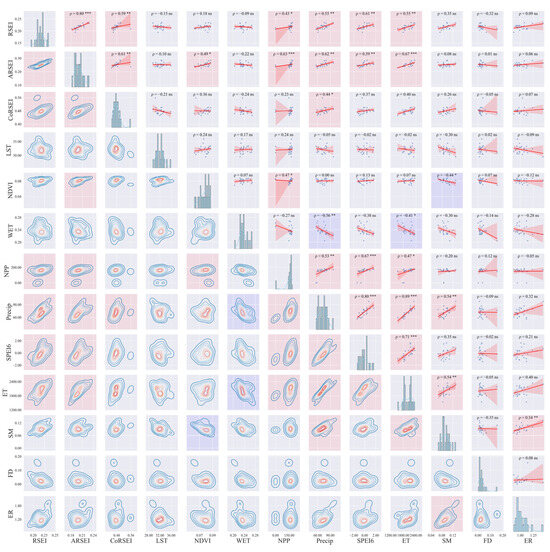
Figure 2.
Correlation Matrix Analysis of Remote Sensing Ecological Indices and Environmental Variables. This figure presents the correlation matrix analysis of 13 ecological and environmental indicators in the Tarim River Basin from 2000 to 2023, including RSEI, ARSEI, CoRSEI, LST, NDVI, WET, NPP, precipitation, SPEI6, evapotranspiration, soil moisture, fire density, and extreme rainfall. The upper triangle displays scatterplots with linear regression trend lines and annotated Spearman correlation coefficients (ρ) along with significance levels (*** p < 0.001; ** p < 0.01; * p < 0.05; ns p ≥ 0.05). Red shading indicates positive correlations, and blue shading indicates negative correlations. The diagonal shows the histogram and kernel density distribution of each individual variable. The lower triangle presents bivariate kernel density estimation (KDE), revealing nonlinear spatial aggregation patterns between variable pairs. In these plots, red regions indicate a high concentration of data points, suggesting that the two variables frequently co-occur within those value ranges.
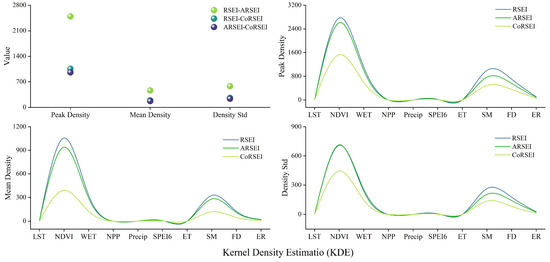
Figure 3.
Comparative KDE analysis of RSEI, ARSEI, and CoRSEI and their associations with environmental factors.
NDVI showed extremely high joint KDEs with RSEI (2772.98), ARSEI (2613.57), and CoRSEI (1532.25), reaffirming its central role. Although the Spearman correlation between NDVI and RSEI was low (ρ = 0.18), high KDE values suggest strong spatial synchronization. NDVI and ARSEI correlated significantly (ρ = 0.49, p < 0.05), indicating ARSEI maintains spatial agreement and improves responsiveness to NDVI variations. Compared to RSEI, ARSEI better detects ecological dynamics driven by vegetation change, consistent with our field verification (Appendix B). CoRSEI showed lower joint density with NDVI, but its Spearman ρ of 0.36 implies it emphasizes non-vegetation factors in ecological quality estimation.
Both RSEI and ARSEI strongly coupled with water-related variables such as WET, soil moisture (SM), and precipitation (Precip). RSEI’s joint KDE with WET and SM were 1093.76 and 1001.71, respectively. ARSEI showed slightly lower densities (WET: 988.50; SM: 770.97), while CoRSEI had weaker coupling (WET: 588.19; SM: 491.07). ARSEI achieved the highest Spearman ρ with precipitation (ρ = 0.62, p < 0.01), exceeding RSEI and CoRSEI, indicating stronger sensitivity to hydrological variables.
RSEI also responded more strongly to disturbance-related variables. Joint KDEs with FireDensity and ExtremeRain were 701.24 and 107.96, higher than CoRSEI (356.88 and 50.71). Although Spearman correlations were not significant, KDE patterns show RSEI better captures ecological degradation from fire and extreme rainfall, suitable for monitoring non-desert regions. ARSEI and CoRSEI were less sensitive to these disturbances.
In summary, RSEI is most suitable for moisture-variable or frequently disturbed environments; ARSEI better captures NDVI and precipitation effects in arid desert systems; and CoRSEI provides a stable framework for background condition extraction and long-term trend assessment.
3.2. Spatiotemporal Dynamics and Evolutionary Trends of CoRSEI (2000–2023)
3.2.1. Spatial Distribution Patterns of CoRSEI
The central Tarim Basin is dominated by extensive desert areas, which exhibit poorer ecological conditions than surrounding regions (Figure 4). In non-desert zones, low RSEI values (0–0.2) are mainly found along desert margins, whereas high values (0.6–1) are scarce and mostly occur at the northern and southern edges. High ARSEI zones (0.8–1) within the desert often border these low RSEI regions, forming ecologically sensitive transitional boundaries that influence desert dynamics.
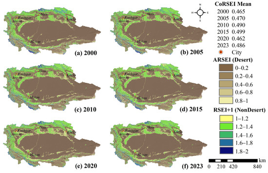
Figure 4.
Spatial distribution map of CoRSEI in the Tarim River Basin from 2000 to 2023.
From 2000 to 2023, the annual mean CoRSEI ranged from 0.45 to 0.56, peaking in 2001 at 0.5585 due to anomalously high RSEI values (1.6758) in non-desert areas, which strongly influenced the composite index (Figure 5). Although fluctuations occurred in other years, the overall trend remained stable. Meanwhile, the proportion of desert area gradually declined from 41.96% in 2000 to 40.55% in 2023, indicating a slow contraction trend. Overall, ecological quality peaked in 2001, whereas the lowest CoRSEI value of 0.4527 occurred in 2009, suggesting stronger degradation pressures that year.
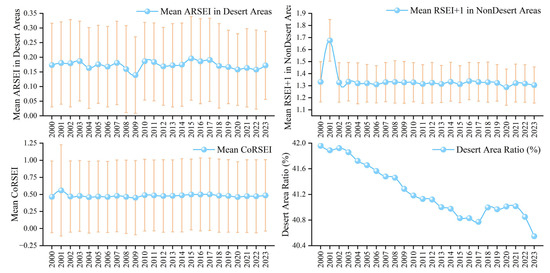
Figure 5.
Annual temporal variation in CORSEI and desert area proportion in the Tarim River Basin from 2000 to 2023.
3.2.2. Spatiotemporal Patterns of CoRSEI Change
Throughout the study period, large portions of the Tarim Basin, particularly the central desert core, show stable ecological conditions, reflecting persistent ecological inertia in hyper-arid environments (Figure 6). Degradation mainly occurs along desert margins and in non-desert mountain foothills and oasis agricultural zones, especially between 2015 and 2020, highlighting the vulnerability of transitional and ecologically sensitive areas. Improvements are most notable in non-desert regions, such as the Tianshan foothills and around oasis cities like Aksu and Korla, during 2005–2010 and 2020–2023, indicating successful ecological restoration or favorable climatic conditions. Desert improvement is observed but is sparse and fragmented, suggesting limited recovery within arid zones.
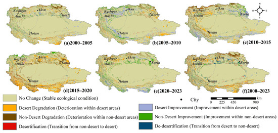
Figure 6.
Spatiotemporal evolution of ecosystem quality in the Tarim River Basin from 2000 to 2023. The maps classify ecological changes into eight categories: stable areas (No Change), desert degradation, non-desert degradation, desertification (transition from non-desert to desert), desert improvement, non-desert improvement, and de-desertification (transition from desert to non-desert).
The cumulative change map (2000–2023) shows that while degradation processes have occurred intermittently across both desert and non-desert areas, ecological improvement—particularly in non-desert regions—has also made substantial progress in the past two decades. These results underscore the dual nature of ecosystem dynamics in arid regions, where both ecological degradation and restoration are spatially heterogeneous and temporally variable.
In the Desert area, the majority of regions consistently fell under the Poor and Fair categories throughout the study period, with only limited improvement observed over time (Figure 7). A small fraction of areas showed slight transitions into higher ecological quality categories; however, these changes appeared transient and often reverted to lower levels, suggesting the ecological fragility and limited resilience of desert ecosystems.
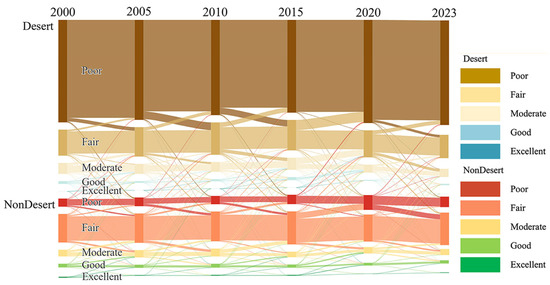
Figure 7.
Dynamic transitions in ecosystem quality across the Tarim River Basin from 2000 to 2023, first distinguished by Desert and Non-Desert regions. Based on the RSEI/ARSEI classification ranges shown in Figure 4, ecological quality is further divided into five levels: Excellent, Good, Moderate, Fair, and Poor. The Sankey diagram illustrates the flows between time periods, depicting changes in ecological status within each region over time.
In contrast, the non-desert area exhibited a more balanced distribution across the quality levels, with moderate to excellent categories persisting and more frequent upward transitions occurring. This pattern reflects a relatively healthier and more stable ecological status in these zones. Transitions from Poor and Fair to higher-quality states were more prominent in non-desert areas, indicating greater potential for ecological restoration and effective management. Overall, the diagram highlights the stark contrast between desert and non-desert regions in terms of ecological quality and stability.
3.2.3. Long-Term Trend Detection and Persistence Analysis of CoRSEI
The spatiotemporal analysis of CoRSEI from 2000 to 2023 (Figure 8a) indicates that most of the study area (68.96%) remained stable, although localized ecological changes were observed, with 1.97% experiencing significant degradation and 1.98% significant improvement. Hurst exponent projections (Figure 8b) suggest that some degraded areas (13.12%) may continue to deteriorate, while a smaller portion (5.72%) could transition from degradation to improvement, indicating potential for ecological recovery. Meanwhile, 70.13% of the area shows uncertain trends, highlighting substantial randomness in long-term ecological dynamics. These results suggest that, although the overall ecosystem is relatively stable, localized changes and high uncertainty underscore the need for continuous monitoring and targeted management interventions. The high proportion of “uncertain” areas (70.13%) may be explained by limitations in the time series length, strong interannual climate variability, and intensive human activities (e.g., water use and land conversion). These factors increase ecological variability and reduce the predictability of long-term trajectories.
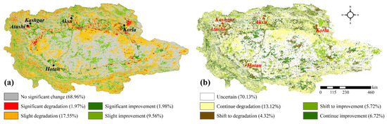
Figure 8.
CoRSEI-based ecological trend classification and future persistence prediction from 2000 to 2023. (a) Trend classification; (b) Future trend prediction.
3.3. Comparative Analysis of Environmental Drivers Influencing ARSEI in Desert Areas and RSEI in Non-Desert Areas
3.3.1. System Coordination Between Environmental Drivers and RSEIs
In the desert region, evapotranspiration (ET) showed the highest coupling degree with ARSEI (C = 0.815), followed by precipitation (Precip, C = 0.736) (Figure 9) and soil moisture (SM, C = 0.713). These moisture-related factors also exhibited relatively high synchronization values (ET: 0.716; Precip: 0.650), indicating that they are not only numerically closely correlated with ecological status but also follow consistent temporal trends.
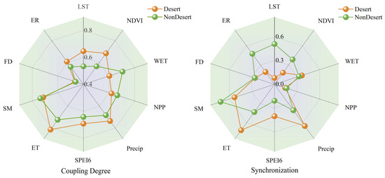
Figure 9.
Coupling and Synchronization Analysis of Environmental Factors and Ecological Indices in Desert and Non-Desert Regions.
In the non-desert region, soil moisture (SM, C = 0.737) and ET (C = 0.725) were the factors most strongly associated with RSEI, with SM exhibiting the highest synchronization (S = 0.715). Land surface temperature (LST) also showed considerable synchronization (S = 0.509), suggesting a significant influence on ecological quality. Vegetation-related factors, such as NDVI and NPP, displayed moderate coupling degrees, indicating that while vegetation status is important, it alone is insufficient to comprehensively characterize regional ecological quality.
3.3.2. Temporal Sensitivity of Ecological Responses to Environmental Drivers
In the desert area, evapotranspiration (ET) consistently showed a strong positive correlation with ARSEI. The ρ values at the 3-, 5-, and 7-year scales were 0.886, 0.87, and 0.83, respectively (Figure 10). The influence of precipitation (Precip) and the Standardized Precipitation Evapotranspiration Index over 6 months (SPEI6) increased with longer temporal scales. Specifically, at the 3-, 5-, and 7-year scales, the ρ values were as follows: Precip: 0.638, 0.704, 0.777; SPEI6: 0.417, 0.49, 0.651. Soil moisture (SM) was positively correlated with ARSEI at the 3-year scale, indicating that soil moisture variations affected ARSEI over shorter periods. Notably, wetness (WET) exhibited significant negative correlations with ecological indices at the 5- and 7-year scales (ρ = −0.49, −0.539).
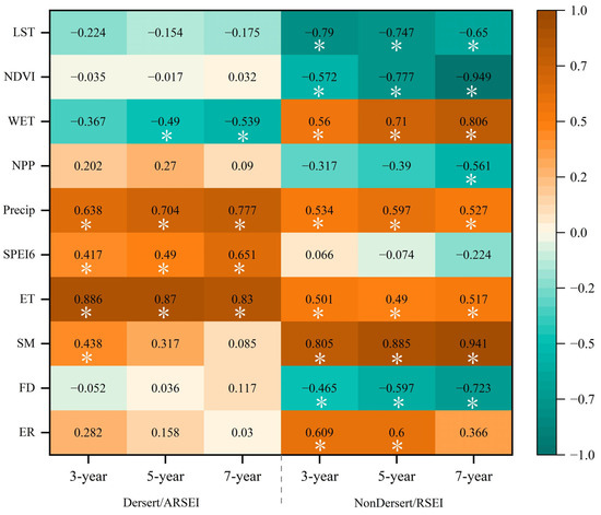
Figure 10.
Spearman rank correlation analyses between ecological indices and environmental factors in desert and non-desert regions using 3-, 5-, and 7-year moving windows (* represents p < 0.05).
In the non-desert region, SM consistently demonstrated a very strong positive correlation with RSEI across all temporal windows (ρ = 0.805, 0.885, 0.941), highlighting the dominant influence of soil moisture on ecological quality in these areas. Additionally, ET, Precip, and WET showed positive correlations with RSEI at the 3-, 5-, and 7-year scales. WET’s impact progressively strengthened over longer time frames, suggesting that sustained soil moisture conditions had a greater positive effect on ecological indices in non-desert regions. Conversely, fire density (FD), NDVI, and land surface temperature (LST) exhibited significant negative correlations with RSEI across all three time scales, with FD and NDVI’s negative influences intensifying over longer periods. Extreme rainfall was positively correlated with RSEI at the 3- and 5-year scales but showed no significant effect at the 7-year scale. In contrast, net primary productivity (NPP) displayed a negative correlation with RSEI at the 7-year scale.
3.3.3. Key Environmental Drivers Determined by Variable Importance Ranking
In the desert region, evapotranspiration (ET), precipitation (Precip), and soil moisture (SM) were the dominant factors influencing the remote sensing ecological index (ARSEI), with variable importance in projection (VIP) values of 1.58, 1.34, and 1.18, respectively (Figure 11). All corresponding regression coefficients were positive, indicating a positive effect of these factors on ARSEI. In contrast, wetness (WET) and the 6-month Standardized Precipitation Evapotranspiration Index (SPEI6) showed negative correlations with the ecological index; although their VIP values exceeded 1, their relationships were inverse. Vegetation indices, such as NDVI and NPP, along with extreme rainfall (ER), land surface temperature (LST), and fire density (FD), exhibited VIP values below 1, suggesting weaker explanatory power in the desert region.
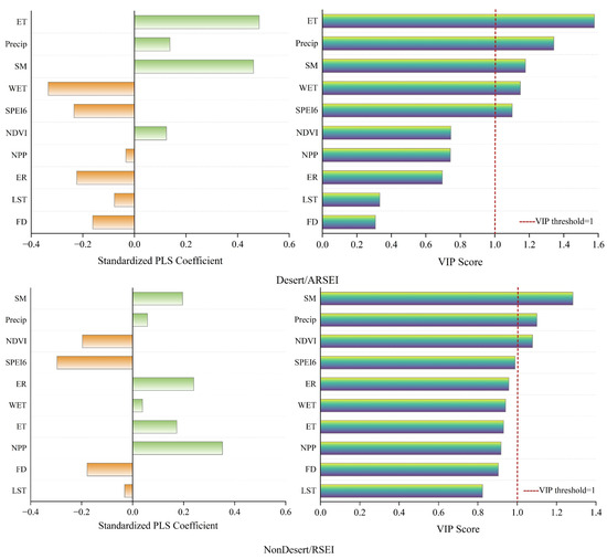
Figure 11.
Insights from PLS-VIP Modeling.
In the non-desert region, all variables had VIP values below 1.3. Soil moisture (SM), precipitation (Precip), and NDVI exerted relatively greater influence, while NPP, despite a slightly lower VIP (0.92), had a substantial positive regression coefficient (0.35), highlighting its important role in ecological status. SPEI6 and fire density (FD) displayed negative regression coefficients, indicating that these stressors adversely affected the remote sensing ecological index.
Overall, the desert ecosystem was primarily constrained by hydrological factors (ET, Precip, and SM), underscoring water availability as the key limiting factor for ecological stability. Conversely, the non-desert ecosystem exhibited more complex interactions between biotic and abiotic factors, with soil moisture, precipitation, and vegetation status jointly influencing ecological dynamics.
3.3.4. Marginal Effects of Environmental Drivers on RSEIs
In the desert region, NDVI, precipitation (Precip), evapotranspiration (ET), and soil moisture (SM) were positively correlated with ARSEI (Figure 12), with partial dependence increasing as the values of these environmental factors rose. Conversely, wetness (WET) showed a negative correlation with ARSEI. Land surface temperature (LST), net primary productivity (NPP), the 6-month Standardized Precipitation Evapotranspiration Index (SPEI6), fire density (FD), and extreme rainfall (ER) exhibited nonlinear responses with ARSEI. Specifically, LST had a weak negative correlation with ARSEI; as LST increased from 32.7 °C to approximately 39.7 °C, ARSEI slightly decreased from about 0.1725 to 0.1719. ARSEI peaked around an NPP value of approximately 136.44 before declining. SPEI6 displayed an inverted U-shaped relationship with ARSEI.
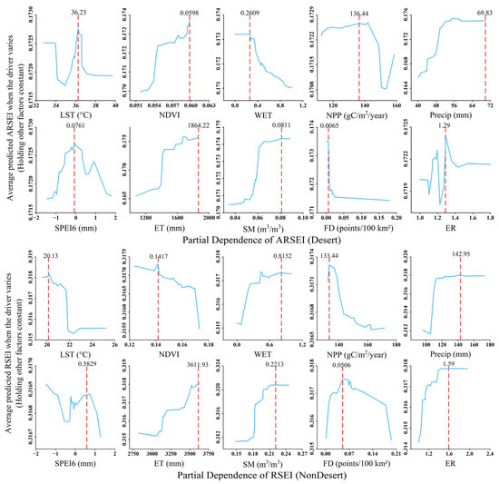
Figure 12.
Partial Dependence Plot. In the Partial Dependence Plot (PDP) analysis, marginal effects reveal the average influence of a single variable on ecological indices (such as RSEI/ARSEI) predictions while holding other variables constant. The vertical dashed lines in each partial dependence plot indicate the key threshold values where the corresponding environmental driver exerts the strongest influence on ARSEI/RSEI, marking the points of strongest ecological responses within the studied arid region.
In the non-desert region, WET, Precip, ET, SM, and ER were positively correlated with RSEI, with partial dependence increasing alongside these environmental factors. In contrast, LST, NDVI, and NPP showed negative correlations with RSEI. SPEI6 exhibited a weak negative correlation with RSEI, while FD presented an inverted U-shaped relationship, showing a slightly positive effect at low values.
4. Discussion
4.1. Adaptability Assessment and Zonal Application Strategy of Multi-Model Remote Sensing Ecological Indices
The RSEI model, characterized by structural stability and a high explanatory power of its first principal component, is well suited for areas with complex ecological drivers, such as urban zones and cultivated lands [6]. However, in extremely arid and sparsely vegetated regions, the contributions of NDVI and NDBSI to the principal component are extremely low, resulting in insufficient ecological information and limited applicability of the model in hyper-arid environments (Table 2). In contrast, the ARSEI model incorporates Albedo, which effectively compensates for the failure of NDVI and NDBSI in desert regions, offering a more ecologically rational structure. As a physically based indicator of surface energy reflectance, Albedo demonstrates stronger ecological sensitivity in high-reflectance environments, whereas the empirically derived NDBSI is prone to misclassification on bare or sandy surfaces, thereby undermining model stability [58].
Overall, in desert regions, where ecological stress is primarily driven by heat and aridity, the ARSEI model is recommended to enhance robustness against ecological degradation. In non-desert areas, characterized by complex ecological drivers and frequent anthropogenic disturbances, the RSEI model remains more appropriate. However, it is worth noting that ARSEI has limited capability in detecting heterogeneous surface structures and human-induced disturbances, suggesting that model selection and application should be tailored to regional characteristics.
From the perspective of model adaptability, a zonal modeling strategy is recommended in practical applications based on land use types and ecological baseline differences. Specifically, RSEI should be applied in non-desert areas, and ARSEI in desert regions. Alternatively, conditional ecological evaluation models can be constructed using NDVI thresholds or land cover classifications to improve ecological logic and spatial applicability. In this study, RSEI and ARSEI exhibited a high degree of consistency, with a maximum joint kernel density (KDE Max) of 2493.83 and a Spearman correlation coefficient of 0.80 (p < 0.001), laying the foundation for the construction of the Composite RSEI (CoRSEI) (Figure 2). CoRSEI demonstrated strong capacity in delineating ecological boundaries and detecting spatial heterogeneity within desert–non-desert ecotones, making it suitable for fine-scale ecological monitoring and zonal management in arid environments.
However, CoRSEI still lags behind RSEI and ARSEI in terms of explaining the ecological functionality of individual environmental factors, indicating a limitation in ecological mechanism representation. Therefore, when applying CoRSEI for ecological quality assessment, it is essential to interpret desert and non-desert zones separately, to avoid masking regional differences and overlooking functional heterogeneity.
The framework is currently validated only in the Tarim Basin. We fully acknowledge that this represents a limitation. Nevertheless, the ARSEI and CoRSEI framework has potential for application in other arid and semi-arid systems for several reasons. First, arid and semi-arid regions share common ecological stressors, including water scarcity, high temperature variability, sparse vegetation, and susceptibility to land degradation. The indicators integrated in ARSEI (e.g., Albedo, NDVI, dryness and greenness indices) are designed to capture these universal features, suggesting potential applicability beyond the Tarim Basin. Second, the PCA-based weighting approach allows the framework to be recalibrated according to local data characteristics, ensuring adaptability to regional environmental conditions. Third, CoRSEI’s conceptual logic, based on desert–non-desert transitions, applies to other regions such as the Sahel, Central Asia, and Southwestern United States, though threshold adjustments may be required. Further validation in other areas is necessary, and future work will aim to test ARSEI and CoRSEI in representative arid and semi-arid systems to evaluate robustness and generalizability.
4.2. Differential Environmental Drivers Response and Spatially Adaptive Remote Sensing Monitoring in Desert and Non-Desert Areas
This study reveals that desert ecosystems are highly sensitive to hydrological factors, including evapotranspiration (ET), precipitation, and soil moisture, with ecological conditions primarily constrained by water availability. Even slight increases in vegetation cover can lead to ecological improvements in minimally disturbed, sparsely vegetated environments, a phenomenon widely observed in arid-region micro-oases and restoration zones [59]. However, moisture accumulation does not necessarily enhance ecological conditions; wetness (WET) exhibits negative effects in desert areas, likely due to surface salinization and groundwater rise caused by water retention, particularly pronounced in low-lying regions [60,61].
In contrast, the non-desert region exhibits more complex ecological regulation mechanisms. NDVI is negatively correlated with ecological status in these areas, likely due to the “greening illusion” caused by urban fringe green spaces, plantations, or monoculture expansion (Figure 13), where increased NDVI does not correspond to improved ecological function [62]. This phenomenon of artificial greening is more prevalent in areas with moderate to high vegetation cover, often leading to misinterpretation of ecological indices [63]. Conversely, wetness (WET) shows a positive effect in the non-desert region, indicating its effectiveness in representing natural moist patches or ecologically favorable zones.
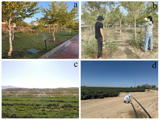
Figure 13.
Typical Scenes of Artificial Greening and Farmland Irrigation in Non-Desert Regions. (a) Urban Green Space Irrigation; (b) Roadside Shelterbelt Irrigation; (c) Farmland Sprinkler Irrigation; (d) Farmland Pipeline Irrigation System.
The observed discrepancies among methods mainly reflect their different focuses: coupling degree and temporal correlation emphasize the synchronization and lagged responses of ecological systems, whereas variable importance ranking and marginal effect analyses highlight the strength and direction of each factor’s influence. These complementary perspectives provide a more comprehensive understanding of environmental drivers and their ecological impacts.
Overall, desert ecosystems are predominantly controlled by water stress, whereas ecological conditions in non-desert regions are jointly regulated by vegetation function, climatic stress, and soil moisture [64,65]. The two regions exhibit opposite ecological response patterns to wetness (WET) and NDVI, underscoring the spatial dependency of ecological variable effects. These findings support the implementation of site-specific remote sensing ecological monitoring strategies: In desert areas, monitoring should emphasize hydrological fluctuations and salinization risks, with management focusing on stabilizing fragile ecosystems, mitigating salinization, and promoting sustainable oasis land use. In non-desert regions, monitoring should integrate productivity and vegetation quality to avoid overreliance on single indicators such as NDVI, while management should prioritize enhancing restoration potential and maintaining ecological quality.
4.3. Differentiated Governance Strategies in the Tarim Basin
The ecological environment of the Tarim region showed an improving trend in 2001, primarily due to the concentrated implementation of ecological projects, including natural forest protection, cropland-to-forest conversion, and the continued promotion of ecological water conveyance to the lower reaches of the Tarim River [66]. Subsequently, hydrological anomalies, salinization, and human activities caused some deterioration, although the overall ecological status remained relatively stable [67]. By 2009, the ecological quality of desert areas had declined, with severe salinization and oasis expansion reducing the ecological buffering capacity [68]. Due to the fragile structure and low resilience of desert ecosystems, they are highly sensitive to disturbances, and degradation can intensify rapidly [69].
Comparisons between desert and non-desert areas reveal clear contrasts. Desert regions maintained low ecological quality over the long term, showing limited variability and short-term improvements that are difficult to sustain, reflecting their inherent vulnerability. In contrast, non-desert areas exhibit a more balanced distribution of ecological grades and greater sustainability. This contrast highlights the need for differentiated ecological governance strategies: desert areas require emphasis on ecosystem stability and vulnerability management, whereas non-desert regions should focus on improving ecological quality and enhancing restoration potential [70].
The evolution of ecosystems follows distinct phase characteristics, making scientific management of transitional zones essential. The ecotone between desert and non-desert regions—termed the ecological transition zone—is highly sensitive (Figure 14). It may serve as either the frontline of desert expansion or a core area of oasis degradation [71]. These zones can be effectively identified using CoRSEI, providing strong technical support for recommendations that ecological governance in desert transition zones should adopt integrated zonal identification, differentiated interventions, and continuous monitoring [72]. In this study, transition zones often show high ARSEI and low RSEI values (Figure 3), reflecting pronounced ecological gradients vulnerable to wind erosion, land use changes, and human activities. Prioritizing these areas for monitoring and management can prevent further desert encroachment and maintain both ecological stability and regional spatial security [73].
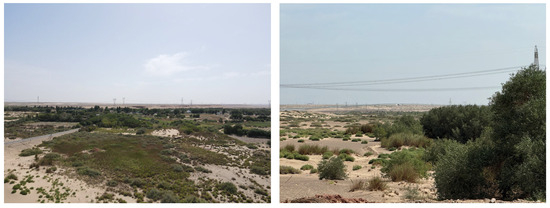
Figure 14.
Ecological transition zone.
In addition, Hurst exponent analysis revealed that 70.13% of the study area shows “uncertain” future ecological trends. This uncertainty is mainly related to the relatively short ecological time series, strong interannual climate variability, and intensive human activities, all of which increase randomness in ecological trajectories and reduce the predictability of long-term changes. From a management perspective, this highlights the need for adaptive and resilient strategies rather than reliance on fixed predictions. High-uncertainty areas should strengthen monitoring, enhance ecosystem recovery capacity, and maintain flexibility in land and water use planning to improve the reliability of long-term ecological governance.
Building on these findings, improved ecological assessment using ARSEI, RSEI, and CoRSEI provides a solid foundation for policy and management decisions. Precise identification of ecologically sensitive zones enables targeted interventions to prevent land degradation and support land degradation neutrality. Furthermore, the spatially explicit information from CoRSEI allows planners to prioritize conservation resources, optimize land use planning, and implement adaptive management strategies that respond dynamically to environmental changes.
5. Conclusions
This study introduces two novel remote sensing ecological indices—ARSEI, optimized for desert ecosystems, and CoRSEI, designed to integrate desert and non-desert ecological assessments. The aim is to enhance the spatial adaptability and environmental responsiveness of ecosystem monitoring in arid regions. Based on a 24-year analysis of the Tarim River Basin, the following conclusions can be drawn:
- (1)
- Performance and Structural Characteristics of the Indices: ARSEI significantly improves sensitivity to vegetation (NDVI) and albedo in hyper-arid environments, making it more effective for characterizing desert ecosystems. CoRSEI, through explicit regional segmentation, effectively captures spatial structural differences and long-term ecological evolution trends between desert and non-desert zones, demonstrating strong temporal stability. While RSEI retains the highest internal consistency and is suitable for detecting abrupt ecological disturbances, ARSEI shows stronger correlations with vegetation and precipitation dynamics, offering advantages in water-limited systems.
- (2)
- Regional Differences in Environmental Drivers: In desert areas, evapotranspiration, precipitation, and soil moisture were identified as the primary positive drivers of ecological conditions. In contrast, in non-desert areas, although soil moisture and precipitation remained important, ecological dynamics were also influenced by vegetation indices (NDVI, NPP) and disturbance-related variables such as fire density and land surface temperature. Some of these factors exhibited negative correlations, indicating more complex ecological response mechanisms.
- (3)
- Long-Term Trends and Monitoring Implications: Analysis of CoRSEI revealed a modest overall improvement in ecological quality across the study area since 2000, accompanied by a gradual reduction in desert areas by approximately 1.41%. However, trend persistence analysis based on the Hurst exponent indicated that most ecological changes lacked sustained directional continuity, highlighting significant uncertainty in future trajectories. Overall, the dual-index framework of ARSEI and CoRSEI provides a spatially differentiated and driver-sensitive methodology for ecological monitoring, offering a robust scientific basis for ecosystem management and restoration in arid regions.
Author Contributions
Conceptualization, Y.C. and Z.H.; methodology, Y.C., L.H. and Y.Z.; software, Y.C., F.L. and J.G.; validation, Y.C., X.C. and W.B.; formal analysis, Y.C. and W.B.; investigation, Y.C. and F.L.; re-sources, Z.H. and L.H.; data curation, Y.C. and J.G.; writing—original draft preparation, Y.C.; writing—review and editing, L.H. and Z.H.; visualization, Y.C. and X.C.; supervision, L.H. and Z.H.; project administration, Z.H. and L.H.; funding acquisition, L.H. and Z.H. All authors have read and agreed to the published version of the manuscript.
Funding
This research was supported by the Third Xinjiang Comprehensive Scientific Expedition Project (Grant No. 2023xjkk0103); the National Natural Science Foundation of China (Grant No. 42301456); and the State Key Laboratory of Geohazard Prevention and Geoenvironment Protection Independent Research Project (Grant No. SKLGP2022Z017).
Data Availability Statement
The original data presented in the study are openly available in: https://doi.org/10.5281/zenodo.17189984.
Acknowledgments
We thank all our colleagues who contributed to this work.
Conflicts of Interest
The authors declare no conflicts of interest.
Abbreviations
The following abbreviations are used in this manuscript:
| RSEI | Remote Sensing Ecological Index |
| ARSEI | Arid-region Remote Sensing Ecological Index |
| CoRSEI | Composite Remote Sensing Ecological Index |
| PCA | Principal Component Analysis |
| TRB | Tarim River Basin |
| LST | Land Surface Temperature |
| NDVI | Normalized Difference Vegetation Index |
| WET | Wetness |
| NDBSI | Normalized Difference Built-up and Soil Index |
| ED | Environmental Drivers |
| NPP | Net Primary Productivity |
| Precip | Precipitation |
| SPEI6 | Standardized Precipitation Evapotranspiration Index |
| ET | Evapotranspiration |
| SM | Soil Moisture |
| FD | Fire Density |
| ER | Extreme Rainfall |
Appendix A. Validation of the Resampling Method
To assess the reliability of the resampling procedure, we designed a dedicated validation experiment focusing on resolutions similar to the datasets used in this study, specifically:
- (1)
- Low-resolution data: 11 km (simulated ERA5-Land soil moisture data);
- (2)
- Medium-low-resolution data: 5.6 km (simulated CHIRPS precipitation data);
- (3)
- Comparative data: 1 km (simulated high-resolution dataset).
The validation adopted a “resampling–back sampling” strategy: each dataset was first resampled to 500 m resolution using bilinear interpolation, and then interpolated back to its original resolution for error evaluation.
From the visual inspection (Figure A1.), the original dataset presents a realistic environmental gradient. The 500 m resampled result retains the overall spatial pattern while providing smoother transitions at boundaries. Most importantly, the back-sampled dataset exhibits a high degree of spatial consistency with the original dataset, suggesting that bilinear interpolation effectively preserves spatial autocorrelation during the resampling–back sampling procedure. To quantify this, 5000 random sample points were extracted to generate the scatter plots used for the linear fitting shown in Figure A2.
This observation is further supported by the quantitative validation results shown in Table A1. All datasets, regardless of resolution, demonstrate high agreement between the original and back-sampled versions, with RMSE values around 6.0, R2 consistently at 0.95, correlation coefficients at 0.975, and negligible biases close to zero. The MAE values (around 4.8) also confirm the small magnitude of deviations. These metrics collectively indicate that the resampling process introduces minimal distortion.
The results confirm that bilinear interpolation is a reliable method for resampling environmental driver datasets. It not only maintains the spatial distribution patterns but also ensures strong statistical consistency with the original data. This reliability is particularly critical for subsequent analyses of environmental drivers, as it guarantees that resampling will not compromise spatial correlations or introduce systematic errors.

Figure A1.
Spatial distribution preservation capacity of the bilinear interpolation method. The numbers on the left indicate pixel coordinate indices, reflecting grid count differences across resolutions. The color bar on the right represents the relative values of the simulated environmental variable.

Table A1.
Validation of the resampling–back sampling strategy across different data resolutions (RMSE = Root Mean Square Error; R2 = Coefficient of Determination; Bias = Mean Error; MAE = Mean Absolute Error). The statistical metrics are derived from the linear fitting results shown in Figure A2.
Table A1.
Validation of the resampling–back sampling strategy across different data resolutions (RMSE = Root Mean Square Error; R2 = Coefficient of Determination; Bias = Mean Error; MAE = Mean Absolute Error). The statistical metrics are derived from the linear fitting results shown in Figure A2.
| Data Type | Original Resolution | RMSE | R2 | Correlation Coefficient | Bias | MAE |
|---|---|---|---|---|---|---|
| ERA5-Land soil moisture (sim.) | 11.0 km | 6.05 | 0.950 | 0.975 | −0.00053 | 4.82 |
| CHIRPS precipitation(sim.) | 5.6 km | 6.04 | 0.950 | 0.975 | 0.0003 | 4.82 |
| Comparative dataset (sim.) | 1.0 km | 6.01 | 0.950 | 0.975 | −0.00001 | 4.79 |

Figure A2.
Linear fitting between original and resampling–back sampling datasets at different resolutions.
Figure A2.
Linear fitting between original and resampling–back sampling datasets at different resolutions.

Appendix B. Field Quadrat Validation
We constructed a 1 m × 1 m vegetation quadrat, which was further divided into 10 × 10 smaller grids. By visually assessing the vegetation coverage within each quadrat (Figure A3), we evaluated the vegetation growth status and, in turn, reflected the ecological condition of the site. At the same time, we calculated the RSEI, ARSEI, and CoRSEI values for each field survey location.
Our results show that ARSEI is more sensitive in detecting vegetation changes in areas with lower vegetation coverage (Table A2), which is consistent with our finding that ARSEI better captures NDVI variations in desert regions. In contrast, for areas with relatively high vegetation coverage, RSEI remains more effective in monitoring ecological changes. Based on this pattern, we integrated ARSEI for desert regions and RSEI for non-desert regions to construct CoRSEI, which provides a more robust tool for monitoring ecological quality dynamics across arid and semi-arid areas.
Table A2.
Actual Vegetation Coverage and the Corresponding RSEI, ARSEI, and CoRSEI Values. Note: The letters in the table correspond to the field survey photographs of vegetation shown in the Figure A3.
Table A2.
Actual Vegetation Coverage and the Corresponding RSEI, ARSEI, and CoRSEI Values. Note: The letters in the table correspond to the field survey photographs of vegetation shown in the Figure A3.
| Figure Panel | Vegetation Coverage | RSEI | ARSEI | CoRSEI |
|---|---|---|---|---|
| a | 35% | 0.028 | 0.137 | 0.137 |
| b | 47% | 0.083 | 0.156 | 0.156 |
| c | 6% | 0.003 | 0.076 | 0.076 |
| d | 0% | 0.022 | 0.031 | 0.031 |
| e | 7% | 0.091 | 0.112 | 0.112 |
| f | 4% | 0.082 | 0.107 | 0.107 |
| g | 8% | 0.107 | 0.169 | 0.169 |
| h | 87% | 0.353 | 0.286 | 1.353 |
| i | 85% | 0.376 | 0.300 | 1.376 |
| j | 92% | 0.395 | 0.310 | 1.395 |
| k | 98% | 0.544 | 0.485 | 1.544 |
| l | 99% | 0.723 | 0.638 | 1.723 |

Figure A3.
Field investigation of vegetation cover. (a–g) Desert regions; (h–l) Non-desert regions.
Figure A3.
Field investigation of vegetation cover. (a–g) Desert regions; (h–l) Non-desert regions.

References
- Zhao, W.; Cheng, G. Review of several problems on the study of eco-hydrological processes in arid zones. Chin. Sci. Bull. 2002, 47, 353–360. [Google Scholar] [CrossRef]
- Wang, Z.; Xiong, H.; Zhang, F.; Qiu, Y.; Ma, C. Sustainable development assessment of ecological vulnerability in arid areas under the influence of multiple indicators. J. Clean. Prod. 2024, 436, 140629. [Google Scholar] [CrossRef]
- Akhtar, M.; Zhao, Y.; Gao, G.; Gulzar, Q.; Hussain, A. Assessment of spatiotemporal variations of ecosystem service values and hotspots in a dryland: A case-study in Pakistan. Land Degrad. Dev. 2022, 33, 1383–1397. [Google Scholar] [CrossRef]
- Wei, L.; Zhong, L.; Yue, Y.; Feng, X.; Li, T.; Song, D.; Zhao, W. Divergent drivers of temporal stability for gravel and sandy desert ecosystems around mobile deserts: Implications for ecosystem conservation and desertification management. Catena 2025, 256, 109088. [Google Scholar] [CrossRef]
- Ajaj, Q.M.; Pradhan, B.; Noori, A.M.; Jebur, M.N. Spatial Monitoring of Desertification Extent in Western Iraq using Landsat Images and GIS. Land Degrad. Dev. 2017, 28, 2418–2431. [Google Scholar] [CrossRef]
- Zheng, Z.; Wu, Z.; Chen, Y.; Guo, C.; Marinello, F. Instability of remote sensing based ecological index (RSEI) and its improvement for time series analysis. Sci. Total Environ. 2022, 814, 152595. [Google Scholar] [CrossRef]
- Verburg, P.H.; Crossman, N.; Ellis, E.C.; Heinimann, A.; Hostert, P.; Mertz, O.; Nagendra, H.; Sikor, T.; Erb, K.-H.; Golubiewski, N.; et al. Land system science and sustainable development of the earth system: A global land project perspective. Anthropocene 2015, 12, 29–41. [Google Scholar] [CrossRef]
- Kiani, P.; Shabani, A.A.; Ahmadi, M. Landscape sustainability indicators for monitoring habitat vulnerability under climate and land use Change: Case studies from four mammal species. Environ. Sustain. Indic. 2025, 26, 100716. [Google Scholar] [CrossRef]
- Xu, H. A remote sensing urban ecological index and its application. Acta Ecol. Sin. 2013, 33, 7853–7862. [Google Scholar] [CrossRef]
- Maimaitituersun, A.; Yang, H.; Aobuliaisan, N.; Maimaitiaili, K.; Ouyang, C. Assessing subtle changes in arid land river basin ecological quality: A study utilizing the PIE engine platform and RSEI. Ecol. Indic. 2025, 170, 113035. [Google Scholar] [CrossRef]
- Zhang, L.; Liu, Q.; Wang, J.; Wu, T.; Li, M. Constructing ecological security patterns using remote sensing ecological index and circuit theory: A case study of the Changchun-Jilin-Tumen region. J. Environ. Manag. 2025, 373, 123693. [Google Scholar] [CrossRef] [PubMed]
- Xin, J.; Yang, J.; Yu, H.; Ren, J.; Yu, W.; Cong, N.; Xiao, X.; Xia, J.; Li, X.; Qiao, Z. Towards ecological civilization: Spatiotemporal heterogeneity and drivers of ecological quality transitions in China (2001–2020). Appl. Geogr. 2024, 173, 103439. [Google Scholar] [CrossRef]
- Shi, S.; Qiu, H.; Ji, S.; Luo, Z. The Combined Effects of Topography and Climate Factors Dominate the Spatiotemporal Evolution of the Ecological Environment in the Yangtze River Economic Belt. Land Degrad. Dev. 2025, 36, 2022–2038. [Google Scholar] [CrossRef]
- Wang, Z.; Chen, T.; Zhu, D.; Jia, K.; Plaza, A. RSEIFE: A new remote sensing ecological index for simulating the land surface eco-environment. J. Environ. Manag. 2023, 326, 116851. [Google Scholar] [CrossRef] [PubMed]
- Li, J.; Zhang, Y.; Yang, L.; Shan, Z. Seasonal variations in ecological environment quality across different geomorphological regions and their response mechanisms to climate change. Sci. Rep. 2025, 15, 26385. [Google Scholar] [CrossRef]
- Lei, X.; Liu, H.; Li, S.; Luo, Q.; Cheng, S.; Hu, G.; Wang, X.; Bai, W. Coupling coordination analysis of urbanization and ecological environment in Chengdu-Chongqing urban agglomeration. Ecol. Indic. 2024, 161, 111969. [Google Scholar] [CrossRef]
- Wang, J.; Ma, J.; Xie, F.; Xu, X. Improvement of remote sensing ecological index in arid regions: Taking Ulan Buh Desert as an example. Ying Yong Sheng Tai Xue Bao (J. Appl. Ecol. China) 2020, 31, 3795–3804. [Google Scholar] [CrossRef]
- Zha, Y.; Gao, J.; Ni, S. Use of normalized difference built-up index in automatically mapping urban areas from TM imagery. Int. J. Remote Sens. 2003, 24, 583–594. [Google Scholar] [CrossRef]
- Weng, Q. Remote sensing of impervious surfaces in the urban areas: Requirements, methods, and trends. Remote Sens. Environ. 2011, 117, 34–49. [Google Scholar] [CrossRef]
- Tsvetsinskaya, E.A.; Schaaf, C.B.; Gao, F.; Strahler, A.H.; Dickinson, R.E. Spatial and temporal variability in Moderate Resolution Imaging Spectroradiometer–derived surface albedo over global arid regions. J. Geophys. Res. Atmos. 2006, 111, D20106. [Google Scholar] [CrossRef]
- Salomon, J.G.; Schaaf, C.; Strahler, A.H.; Gao, F.; Jin, Y. Validation of the MODIS bidirectional reflectance distribution function and albedo retrievals using combined observations from the aqua and terra platforms. IEEE Trans. Geosci. Remote Sens. 2006, 44, 1555–1565. [Google Scholar] [CrossRef]
- Jin, Y.; Schaaf, C.B.; Woodcock, C.E.; Gao, F.; Li, X.; Strahler, A.H.; Lucht, W.; Liang, S. Consistency of MODIS surface bidirectional reflectance distribution function and albedo retrievals: 2. Validation. J. Geophys. Res. Atmos. 2003, 108, 4159. [Google Scholar] [CrossRef]
- Normand, J.C.L.; Heggy, E. Measuring soil moisture change and surface erosion from sparse rainstorms in hyper-arid terrains. Int. J. Appl. Earth Obs. Geoinf. 2025, 142, 104642. [Google Scholar] [CrossRef]
- Brunelli, B.; Mancini, F. Comparative analysis of SAOCOM and Sentinel-1 data for surface soil moisture retrieval using a change detection method in a semiarid region (Douro River’s basin, Spain). Int. J. Appl. Earth Obs. Geoinf. 2024, 129, 103874. [Google Scholar] [CrossRef]
- Alsafadi, K.; Bashir, B.; Mohammed, S.; Abdo, H.G.; Mokhtar, A.; Alsalman, A.; Cao, W. Response of Ecosystem Carbon–Water Fluxes to Extreme Drought in West Asia. Remote Sens. 2024, 16, 1179. [Google Scholar] [CrossRef]
- Wu, L.; Li, C.; Xie, X.; He, Z.; Wang, W.; Zhang, Y.; Wei, J.; Lv, J. The impact of increasing land productivity on groundwater dynamics: A case study of an oasis located at the edge of the Gobi Desert. Carbon Balance Manag. 2020, 15, 7. [Google Scholar] [CrossRef]
- Johnson, S.; Ivanovich, C.; Horton, R.M.; Ting, M.; Kornhuber, K.; Lesk, C. Temporal connections between extreme precipitation and humid heat. Environ. Res. Lett. 2024, 19, 114076. [Google Scholar] [CrossRef]
- Zhang, M.; Zhang, H.; Deng, W.; Yuan, Q. Assessment of Habitat Quality in Arid Regions Incorporating Remote Sensing Data and Field Experiments. Remote Sens. 2024, 16, 3648. [Google Scholar] [CrossRef]
- Liu, S.a.; Sun, T.; Ciais, P.; Zhang, H.; Fang, J.; Fang, J.; Gemechu, T.M.; Chen, B. Assessing Habitat Quality on Synergetic Land-Cover Dataset Across the Greater Mekong Subregion over the Last Four Decades. Remote Sens. 2025, 17, 1467. [Google Scholar] [CrossRef]
- Jiang, N.; Zhang, Q.; Zhang, S.; Zhao, X.; Cheng, H. Spatial and temporal evolutions of vegetation coverage in the Tarim River Basin and their responses to phenology. Catena 2022, 217, 106489. [Google Scholar] [CrossRef]
- Tang, C.; Li, Q.; Tao, H.; Aihemaiti, M.; Mu, Z.; Jiang, Y. Evaluation and driving factors of ecological environment quality in the Tarim River basin based on remote sensing ecological index. PeerJ 2024, 12, e18368. [Google Scholar] [CrossRef] [PubMed]
- Ling, H.; Guo, B.; Zhang, G.; Xu, H.; Deng, X. Evaluation of the ecological protective effect of the “large basin” comprehensive management system in the Tarim River basin, China. Sci. Total Environ. 2019, 650, 1696–1706. [Google Scholar] [CrossRef]
- Running, S.W.; Nemani, R.R.; Ann, H.F.; Maosheng, Z.; Matt, R.; Hirofumi, H. A Continuous Satellite-Derived Measure of Global Terrestrial Primary Production. Bioscience 2004, 54, 547–560. [Google Scholar] [CrossRef]
- Abatzoglou, J.T.; Dobrowski, S.Z.; Parks, S.A.; Hegewisch, K.C. TerraClimate, a high-resolution global dataset of monthly climate and climatic water balance from 1958–2015. Sci. Data 2018, 5, 170191. [Google Scholar] [CrossRef]
- Muñoz-Sabater, J.; Dutra, E.; Agustí-Panareda, A.; Albergel, C.; Arduini, G.; Balsamo, G.; Boussetta, S.; Choulga, M.; Harrigan, S.; Hersbach, H. ERA5-Land: A state-of-the-art global reanalysis dataset for land applications. Earth Syst. Sci. Data Discuss. 2021, 13, 4349–4383. [Google Scholar] [CrossRef]
- Giglio, L.; Schroeder, W.; Justice, C.O. The collection 6 MODIS active fire detection algorithm and fire products. Remote Sens. Environ. 2016, 178, 31–41. [Google Scholar] [CrossRef]
- Yang, J.; Huang, X. The 30 m annual land cover dataset and its dynamics in China from 1990 to 2019. Earth Syst. Sci. Data 2021, 13, 3907–3925. [Google Scholar] [CrossRef]
- Liang, S. Narrowband to Broadband Conversions of Land Surface Albedo I Algorithms. Remote Sens. Environ. 2001, 76, 213–238. [Google Scholar] [CrossRef]
- Liang, S.; Shuey, C.J.; Russ, A.L.; Fang, H.; Chen, M.; Walthall, C.L.; Daughtry, C.S.T.; Hunt, R. Narrowband to broadband conversions of land surface albedo: II. Validation. Remote Sens. Environ. 2003, 84, 25–41. [Google Scholar] [CrossRef]
- Tucker, C.J. Red and photographic infrared linear combinations for monitoring vegetation. Remote Sens. Environ. 1979, 8, 127–150. [Google Scholar] [CrossRef]
- Lobser, S.E.; Cohen, W.B. MODIS tasselled cap: Land cover characteristics expressed through transformed MODIS data. Int. J. Remote Sens. 2007, 28, 5079–5101. [Google Scholar] [CrossRef]
- Vicente-Serrano, S.M.; Beguería, S.; López-Moreno, J.I. A Multiscalar Drought Index Sensitive to Global Warming: The Standardized Precipitation Evapotranspiration Index. J. Clim. 2010, 23, 1696–1718. [Google Scholar] [CrossRef]
- World Meteorological Organization (WMO). Guidelines on Analysis of Extremes in a Changing Climate in Support of Informed Decisions for Adaptation (WMO-TD No. 1500); Expert Team on Climate Change Detection and Indices (ETCCDI): Geneva, Switzerland, 2009. [Google Scholar]
- Silverman, B.W. Series Density Estimation for Statistics and Data Analysis; Chapman and Hall: New York, NY, USA, 1986. [Google Scholar]
- Sen, P.K. Estimates of the Regression Coefficient Based on Kendall’s Tau. J. Am. Stat. Assoc. 1968, 63, 1379–1389. [Google Scholar] [CrossRef]
- Wang, X.; Li, T.; Ikhumhen, H.O.; Sá, R.M. Spatio-temporal variability and persistence of PM2.5 concentrations in China using trend analysis methods and Hurst exponent. Atmos. Pollut. Res. 2022, 13, 101274. [Google Scholar] [CrossRef]
- Mann, H.B. Nonparametric test against trend. Econometrica 1945, 13, 245–259. [Google Scholar] [CrossRef]
- Kendall, M.G. SeriesRank Correlation Methodsrank Correlation Methods; Griffin: London, UK, 1975. [Google Scholar]
- Hurst, H.E. Long-Term Storage Capacity of Reservoirs. Trans. Am. Soc. Civ. Eng. 1951, 16, 770–799. [Google Scholar] [CrossRef]
- Mandelbrot, B.B.; Wallis, J.R. Robustness of the rescaled range R/S in the measurement of noncyclic long run statistical dependence. Water Resour. Res. 1969, 5, 967–988. [Google Scholar] [CrossRef]
- Mateusz, T. Evaluation of coupling coordination degree and convergence behaviour of local development: A spatiotemporal analysis of all Polish municipalities over the period 2003–2019. Sustain. Cities Soc. 2021, 71, 102992. [Google Scholar] [CrossRef]
- Kou, L.; Wang, X.; Wang, H.; Wang, X.; Hou, Y. Spatiotemporal analysis of ecological benefits coupling remote sensing ecological index and ecosystem services index. Ecol. Indic. 2024, 166, 112420. [Google Scholar] [CrossRef]
- Zhang, J.; Zhou, Q.; Cao, M.; Liu, H. Spatiotemporal Change of Eco-Environmental Quality in the Oasis City and Its Correlation with Urbanization Based on RSEI: A Case Study of Urumqi, China. Sustainability 2022, 14, 9227. [Google Scholar] [CrossRef]
- Jia, J.; Deng, H.; Duan, J.; Zhao, J. Analysis of the major drivers of the ecological footprint using the STIRPAT model and the PLS method—A case study in Henan Province, China. Ecol. Econ. 2009, 68, 2818–2824. [Google Scholar] [CrossRef]
- Farrés, M.; Platikanov, S.; Tsakovski, S.; Tauler, R. Comparison of the variable importance in projection (VIP) and of the selectivity ratio (SR) methods for variable selection and interpretation. J. Chemom. 2015, 29, 528–536. [Google Scholar] [CrossRef]
- Benjamin, M.; Mostafa, Q.E.; Benoît, J. Extension and significance testing of Variable Importance in Projection (VIP) indices in Partial Least Squares regression and Principal Components Analysis. Chemom. Intell. Lab. Syst. 2023, 242, 104986. [Google Scholar] [CrossRef]
- Friedman, J.H. Greedy Function Approximation: A Gradient Boosting Machine. Ann. Stat. 2001, 29, 1189–1232. [Google Scholar] [CrossRef]
- Liu, Y.; Wang, J.; Ding, J.; Zhang, Z.; Liu, Z.; Zhang, Z.; Zhang, J.; Shi, L. Dynamic Monitoring of Ecological Environmental Quality in Arid and Semi-Arid Regions: Disparities Among Central Asian Countries and Analysis of Key Driving Factors. Remote Sens. 2025, 17, 17111825. [Google Scholar] [CrossRef]
- Zhou, W.; Li, C.; Wang, S.; Ren, Z.; Stringer, L.C. Effects of vegetation restoration on soil properties and vegetation attributes in the arid and semi-arid regions of China. J. Environ. Manag. 2023, 343, 118186. [Google Scholar] [CrossRef]
- Wang, Y.; Zhao, Y.; Yan, L.; Deng, W.; Zhai, J.; Chen, M.; Zhou, F. Groundwater regulation for coordinated mitigation of salinization and desertification in arid areas. Agric. Water Manag. 2022, 271, 107758. [Google Scholar] [CrossRef]
- Wang, Y.; Chen, M.; Yan, L.; Yang, G.; Ma, J.; Deng, W. Quantifying Threshold Water Tables for Ecological Restoration in Arid Northwestern China. Ground Water 2020, 58, 132–142. [Google Scholar] [CrossRef] [PubMed]
- Qu, S.; Jiang, Y.; Gao, J.; Cao, Q.; Wang, L.; Zhang, Y.; Huang, F. Spatial-temporal evolution and driving factors of ecosystem services trade-offs and synergies in karst areas from a geospatial perspective. Dev. Degrad. Dev. 2024, 35, 3448–3460. [Google Scholar] [CrossRef]
- Martinez, A.d.l.I.; Labib, S.M. Demystifying normalized difference vegetation index (NDVI) for greenness exposure assessments and policy interventions in urban greening. Environ. Res. 2023, 220, 115155. [Google Scholar] [CrossRef]
- McHugh, T.A.; Compson, Z.; van Gestel, N.; Hayer, M.; Ballard, L.; Haverty, M.; Hines, J.; Irvine, N.; Krassner, D.; Lyons, T.; et al. Climate controls prokaryotic community composition in desert soils of the southwestern United States. FEMS Microbiol. Ecol. 2017, 93, fix116. [Google Scholar] [CrossRef]
- Zhang, M.; Luo, Y.; Yan, Z.; Chen, J.; Eziz, A.; Li, K.; Han, W. Resorptions of 10 mineral elements in leaves of desert shrubs and their contrasting responses to aridity. J. Plant Ecol. 2018, 12, 358–366. [Google Scholar] [CrossRef]
- Yang, H.; Mu, S.; Li, J. Effects of ecological restoration projects on land use and land cover change and its influences on territorial NPP in Xinjiang, China. Catena 2014, 115, 85–95. [Google Scholar] [CrossRef]
- Chen, Y.; Xu, C.; Chen, Y.; Liu, Y.; Li, W. Progress, Challenges and Prospects of Eco-Hydrological Studies in the Tarim River Basin of Xinjiang, China. Environ. Manag. 2013, 51, 138–153. [Google Scholar] [CrossRef]
- Zhang, F.; Tiyip, T.; Feng, Z.; Kung, H.T.; Johnson, V.; Ding, J.; Tashpolat, N.; Sawut, M.; Gui, D. Spatio-temporal patterns of land use/cover changes over the past 20 years in the middle reaches of the Tarim River, Xinjiang, China. Land Degrad. Dev. 2015, 26, 284–299. [Google Scholar] [CrossRef]
- Yu, X.; Lei, J.; Gao, X. An over review of desertification in Xinjiang, Northwest China. J. Arid Land 2022, 14, 1181–1195. [Google Scholar] [CrossRef]
- Singh, G.; Sharma, S. Desert Ecology and Functional Aspects of Desert Ecosystems. In Textbook of Forest Science; Springer Nature Singapore: Singapore, 2025; pp. 227–251. [Google Scholar]
- Wang, T.; Chen, G.; Zhao, H.; Xiao, H. Aeolian Desertification Status and Its Control in China. In Global Degradation of Soil and Water Resources: Regional Assessment and Strategies; Springer Nature Singapore: Singapore, 2022; pp. 199–220. [Google Scholar]
- Gao, J.; Wang, Y.; Zou, C.; Xu, D.; Lin, N.; Wang, L.; Zhang, K. China’s ecological conservation redline: A solution for future nature conservation. Ambio 2020, 49, 1519–1529. [Google Scholar] [CrossRef] [PubMed]
- Chen, Y.; Fang, G.; Li, Z.; Zhang, X.; Gao, L.; Elbeltagi, A.; Shaer, H.E.; Duan, W.; Wassif, O.M.A.; Li, Y.; et al. The Crisis in Oases: Research on Ecological Security and Sustainable Development in Arid Regions. Annu. Rev. Environ. Resour. 2024, 49, 1–20. [Google Scholar] [CrossRef]


Disclaimer/Publisher’s Note: The statements, opinions and data contained in all publications are solely those of the individual author(s) and contributor(s) and not of MDPI and/or the editor(s). MDPI and/or the editor(s) disclaim responsibility for any injury to people or property resulting from any ideas, methods, instructions or products referred to in the content. |
© 2025 by the authors. Licensee MDPI, Basel, Switzerland. This article is an open access article distributed under the terms and conditions of the Creative Commons Attribution (CC BY) license (https://creativecommons.org/licenses/by/4.0/).