Near-Real-Time Turbidity Monitoring at Global Scale Using Sentinel-2 Data and Machine Learning Techniques

Highlights

What are the main findings?

• We have developed a machine-learning algorithm able to quantify high-turbid environments.
• We use open-source and free databases to train the model and open-source and free tools to develop it, which makes it easily replicable and transferable.

What are the implications of the main findings?

• The social impact of our work implies improved monitoring of areas with high turbidity, which can lead to a better understanding and use of forecasting.
• Ocean color and water quality communities can take advantage of the lessons learned for developing new products or services.

Abstract

Reliable global turbidity monitoring is crucial for water resource management, yet existing satellite-based methods face limitations in accuracy, generalization, and scalability across diverse aquatic environments. This study presents a robust, globally applicable turbidity estimation model using Sentinel-2 imagery and a machine-learning approach, developed based on harmonized global open-source datasets (GLORIA and MAGEST; turbidity range: 0–2200 FNU) encompassing 68 lakes, 2 rivers, 2 estuaries, and 11 coastal oceans across 17 countries. Among the evaluated machine-learning models, gradient boosting regression demonstrated the best performance, achieving a high correlation (r: 0.95) with minimal bias (1.32 FNU) and robust generalization across all water types, outperforming existing turbidity models when evaluated on the same test dataset. Shapley Additive exPlanations-based model interpretability identified the Rrs865/Rrs560 ratio as the dominant predictor, with critical contributions from Rrs783, Rrs665, and Rrs865. The model’s performance is evaluated across various optical water types and aquatic systems in diverse geographical settings, showcasing its robustness in sediment-rich and highly turbid environments that underscores its suitability for reliable turbidity monitoring after severe storms or extreme precipitation. Additionally, innovative automated pipelines integrated within a scientific exploitation platform facilitate scalable and near-real-time operational monitoring. This methodological integration provides a significant advancement in satellite-based turbidity monitoring, enabling informed water quality management under diverse environmental and climatic conditions.

1. Introduction

Turbidity, the cloudiness of water caused by suspended particles, serves as a critical indicator of aquatic ecosystem health and water resource sustainability. This optical property reflects both natural processes (river discharge, wave-induced resuspension, erosion, phytoplankton blooms) and anthropogenic pressures (dredging, construction, agricultural runoff), making it indispensable for water resource management across the globe. Whether caused by natural or anthropogenic disturbances, turbidity profoundly influences aquatic life by altering light penetration, thermal stratification, and nutrient cycling. Elevated turbidity levels trigger cascading ecological effects: reduced light penetration impairs photosynthesis and primary productivity, disrupted thermal stratification alters oxygen distribution, and increased nutrient availability may initiate harmful algal blooms, ultimately degrading ecosystem resilience and water security [1,2,3,4,5]. Climate change further exacerbates these impacts through intensified precipitation patterns, increased storm frequency, and accelerated sea-level rise, driving unprecedented sediment mobilization and turbidity episodes across coastal and inland waters [6,7,8,9,10]. As anthropogenic pressures and climate variability intensify, robust turbidity monitoring at relevant spatial and temporal scales has become essential for predicting ecosystem responses and implementing effective mitigation strategies.

Traditional in situ turbidity measurements, while accurate, cannot meet the spatiotemporal demands of modern water resource management. These point-based observations are resource-intensive, logistically challenging in remote regions, and inadequate for capturing episodic events or large-scale disturbances. Satellite remote sensing emerged as a compelling alternative, offering synoptic, repeated observations across vast areas. Early satellite missions, such as Sea-Viewing Wide Field-of-view Sensor (SeaWiFS), Moderate Resolution Imaging Spectroradiometer (MODIS), and Medium Resolution Imaging Spectrometer (MERIS), demonstrated turbidity monitoring potential [11,12,13,14]; however, their coarse spatial resolution (250–1000 m) rendered them inadequate for smaller water bodies and complex coastal zones where fine spatial details are necessary.

The Sentinel-2 MultiSpectral Instrument (MSI) transformed this landscape with 10 m spatial resolution and 5-day revisit frequency, enabling detailed assessments at management-relevant scales [15,16,17,18,19,20]. Yet despite these technological advances, a critical gap persists between algorithm innovation and operational implementation. Current turbidity algorithms remain largely confined to specific regions, sensors, or turbidity ranges, lacking the versatility required for global deployment (

Table 1. Summary of existing satellite-based turbidity algorithms showing their regional scope, sensor specifications, and operational turbidity ranges.

Algorithms	Study Region	Satellites/Sensors (Operational Period)	Turbidity Levels
Semi-empirical single-band algorithm using Rrs859 for high turbidity, and Rrs645 for medium to low turbidity [13]	Southern North Sea, French Guyana, Scheldt, Gironde, Rio Plata	MERIS (2002–2012), MODIS (1999–Present), SeaWiFS (1997–2010)	1–1000 FNU *
Single band algorithm using Rrs842 and Rrs665 [21]	Gironde Estuary, France	Pléiades (2011–Present)	200–900 FNU
Multi-conditional algorithm using Rrs665 and Rrs704 [17]	Guadalquivir Estuary, Spain	Sentinel-2 (2015–Present)	0–600 FNU
Normalized difference turbidity index [22]	Panchet Hill Dam, India	Landsat 5 (1984–2013), Landsat 8 (2013–Present)	<700 FNU
Machine learning [15,23]	Taihu Lake, China; North Tyrrhenian Sea, Italy	Sentinel-2 (2015–Present), Landsat 8/9 (2013–Present)	0–200; 0–30 FNU
Generalized additive models [24]	Doñana Marshes, Spain	Landsat 5 (1984–2013), Landsat 7 (1999–Present)	1–500 FNU
CMEMS [25]	European Seas	Sentinel-2 (2015–Present)	-

* FNU denotes Formazin Nephelometric Units.

). Empirical and semi-empirical models, while successful within their design parameters, fail when confronted with optical conditions beyond their training domains. Even the most widely adopted global turbidity model [13], though more robust within its design parameters, cannot address extreme turbidity conditions common in highly dynamic riverine-estuarine environments [17].

The limitations of existing approaches (Table 1) stem from their reliance on simplified spectral relationships that cannot capture the full complexity of turbidity’s optical signatures across diverse aquatic environments. Machine-learning (ML) techniques offer a promising alternative, with their ability to model complex, nonlinear relationships and adapt to varied optical conditions [15,23,26,27]. However, leveraging this potential requires comprehensive training datasets that span the global aquatic conditions, which have historically been unattainable.

Recent community datasets—GLORIA (GLObal Reflectance community dataset for Imaging and optical sensing of Aquatic environments) and MAGEST (Monitoring the water quality of the Gironde Estuary)—provide unprecedented coverage of in situ radiometry and co-located water quality measurements (i.e., turbidity, among others) across diverse geographic regions and water types [28,29]. While these datasets offer valuable resources, they also present significant challenges due to measurement inconsistencies, methodological variations, and gaps in turbidity observations that require careful harmonization and quality control to ensure reliable model development.

This study presents a comprehensive solution to these challenges by developing a globally applicable turbidity monitoring system that bridges the gap between methodological innovation and operational implementation. Our approach integrates Sentinel-2 observations with advanced ML techniques, trained on rigorously harmonized global datasets to achieve unprecedented monitoring capabilities across a wide turbidity range (0–2200 FNU). We address the following critical challenges: (1) establishing robust data curation approach for merging heterogeneous in situ measurements with satellite observations; (2) developing ML models capable of accurate predictions across diverse optical environments, including extreme turbidity conditions previously beyond algorithmic reach; (3) ensuring model transparency and interpretability through explainable Artificial Intelligence (AI) techniques, i.e., SHapley Additive exPlanations (SHAP) [30] that reveal model’s physical basis of spectral-turbidity relationships; and (4) implementing comprehensive uncertainty quantification. Furthermore, recognizing the operational demand for timely environmental insights, this study presents an innovative automated processing framework that transforms our methodological innovations into practical monitoring tools. Leveraging containerized computing architecture (Docker, v4.44.2 (202017)) and orchestration technologies (Kubernetes, v1.24.3), our system enables near-real-time turbidity monitoring at global scales while maintaining the flexibility to incorporate future improvements and additional data sources. Thus, by effectively advancing the current capabilities of satellite-based extreme turbidity monitoring, as well as bridging methodological innovation with practical applicability, this study presents a high-resolution (10 m) satellite-based turbidity monitoring system, essential for managing aquatic resources under accelerating environmental change.

2. Materials and Methods

2.1. Dataset Integration and Quality Control

This study integrated two complementary datasets to achieve comprehensive global turbidity coverage. The GLORIA dataset (https://doi.org/10.1594/PANGAEA.948492, accessed 22 March 2023) provided 7572 hyperspectral remote sensing reflectance (Rrs, sr⁻¹) measurements spanning 350–900 nm at 1 nm resolution, with co-located turbidity, total suspended solids (TSS), Secchi-depth transparency (SDT), and chlorophyll-a (Chl-a) measurements from lakes, rivers, estuaries, and coastal oceans worldwide [28]. The MAGEST dataset (https://magest.oasu.u-bordeaux.fr/index.php, accessed 19 August 2024) contained 2581 direct turbidity measurements from the Gironde River Estuary, France, a highly turbid and sediment-rich system, providing critical training data for extreme conditions [29]. Together, these datasets spanned turbidity levels from 0 to 2200 FNU across diverse aquatic environments.

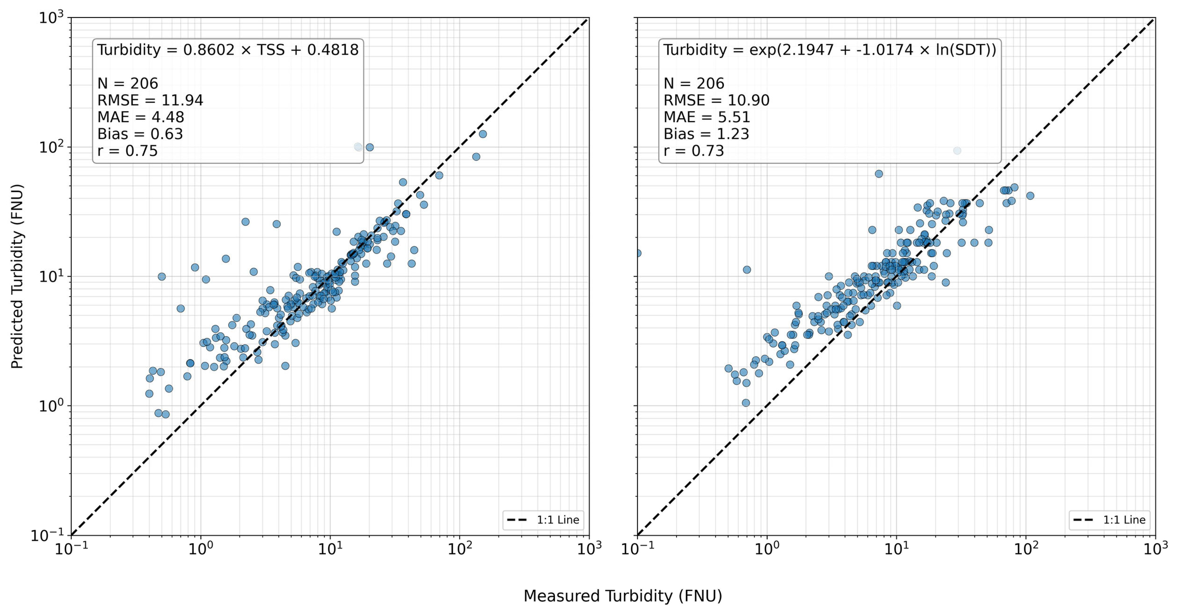
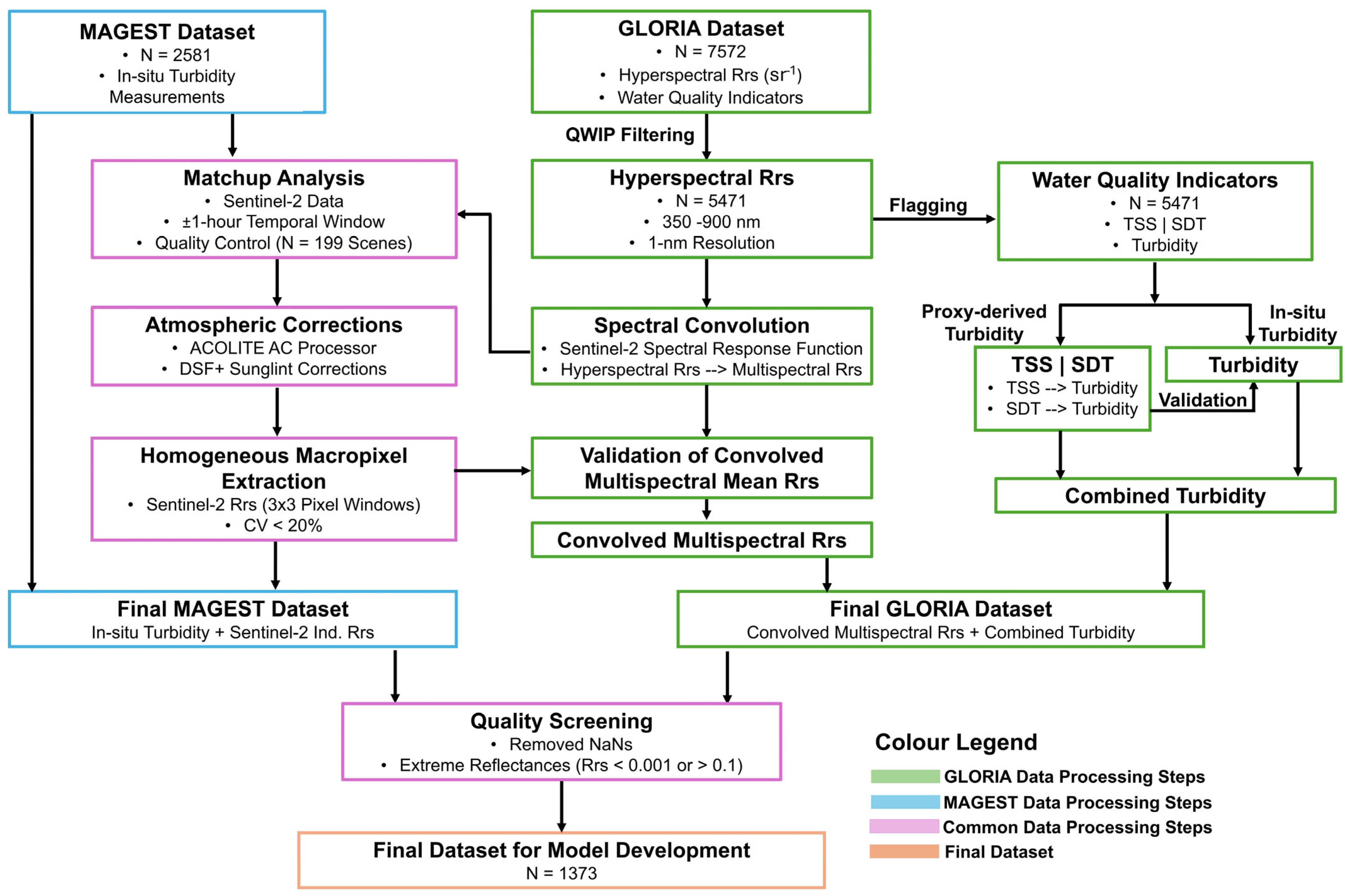
Quality control employed the Quality Water Index Polynomial (QWIP) metric [31] to identify and remove optically inconsistent spectra from GLORIA, reducing the datasets to 5471 valid observations. For observations lacking direct turbidity measurements, we developed predictive models using co-located parameters. Linear regression converted TSS to turbidity (y = 0.86x + 0.48; root mean squared error (RMSE) = 11.94 FNU, correlation coefficient (r) = 0.75) [32], while power regression transformed SDT values (y = exp(2.19 − 1.02ln(x)); RMSE = 10.90 FNU, r = 0.73) [33]. These models, developed using 80% of paired observations and validated on the remaining 20%, demonstrated acceptable predictive performance as shown in

Table 2. Performance metrics for turbidity estimation from TSS and SDT using the test dataset (n = 206).

Model	Equation	Root Mean Squared Error (RMSE), FNU	Mean Absolute Error (MAE), FNU	Bias FNU	Correlation Coefficient (r)
TurbidityTSS	y = 0.86x + 0.48	11.94	4.48	0.63	0.75
TurbiditySDT	y = exp(2.19 − 1.02ln(x))	10.90	5.51	1.23	0.73

and Figure A1. Therefore, these in situ proxy-derived turbidity values were combined with direct in situ available measurements to maximize data coverage across the turbidity spectrum. The MAGEST dataset, consisting entirely of field turbidity measurements, required no proxy estimation, thus providing direct data for model training in the extreme turbidity range.

2.2. Hyperspectral to Multispectral Conversion

Sentinel-2 equivalent reflectances were derived from GLORIA in situ hyperspectral measurements through the spectral response function (SRF) [34] convolution, enabling comparison between in situ-convolved and satellite-derived reflectances. The Sentinel-2 SRF characterizes the wavelength-dependent sensitivity of each MSI band, accounting for the detector’s spectral response across its operational range. The convolution process transformed continuous hyperspectral Rrs measurements (sr⁻¹) at 1 nm resolution into discrete multispectral bands corresponding to Sentinel-2A’s spectral configuration. For each band i, normalized SRF weights were first computed as:

Ŝi(λj) = Si(λj)/Σ_j Si(λj)

(1)

where Si(λj) represents the SRF value at wavelength λj within the band’s range [λi, min, λi, max], and the summation extends over all wavelengths within this range. The convolved Sentinel-2 reflectance for band i was then calculated as:

Ri = Σ_j Ŝi(λj). Rrs(λj)

(2)

The resulting Sentinel-2 equivalent reflectances maintained spectral fidelity while accounting for the instrument’s specific optical characteristics, enabling robust algorithm development using the GLORIA dataset. Only bands within GLORIA’s spectral range (350–900 nm) were retained for analysis, ensuring that all the convolved values were based on measured data.

2.3. Satellite Data Processing

Sentinel-2 Level-1C imagery was acquired through the Copernicus Data Space Ecosystem (https://dataspace.copernicus.eu/, accessed 1 March 2023 onwards) API (Application Programming Interface) for locations and times matching in situ observations. A ±1 h temporal window relative to in situ sampling was applied to minimize temporal discrepancies between satellite and field measurements. Initial acquisition yielded 259 scenes (139 GLORIA, 120 MAGEST), which underwent visual screening using true color composites to identify and exclude images affected by clouds, haze, fog, or strong sun-glint, retaining 199 scenes (101 GLORIA, 98 MAGEST).

Atmospheric correction was performed using the dark spectrum fitting (DSF) algorithm with sun-glint correction implemented in ACOLITE (v20231023) [35], generating 10 m resolution Rrs products. At each sampling location, 3 × 3 pixel windows were extracted and subjected to quality filtering: z-score outlier removal eliminated anomalous pixels, while coefficient of variation (CV) screening retained only homogeneous windows (CV < 20%) [36] across all bands to ensure spatial consistency. For GLORIA locations, mean reflectances were computed from valid pixels within each window and used for validating the convolved spectra derived in Section 2.2. Strong correlations were observed across all bands (r = 0.52–0.93), with the highest agreement for Rrs704, Rrs665, and Rrs560 (Figure 1). RMSE values remained consistently low (0.004–0.005 sr⁻¹) with minimal positive biases (0.0008–0.0029 sr⁻¹), indicating strong agreement and validating the conversion approach. In contrast, MAGEST extraction meeting homogeneity criteria retained all valid pixels, maximizing turbidity-reflectance pairs for model training. In this case, given the homogeneity threshold (CV < 20%), pixel-level variation was considered negligible for this dataset.

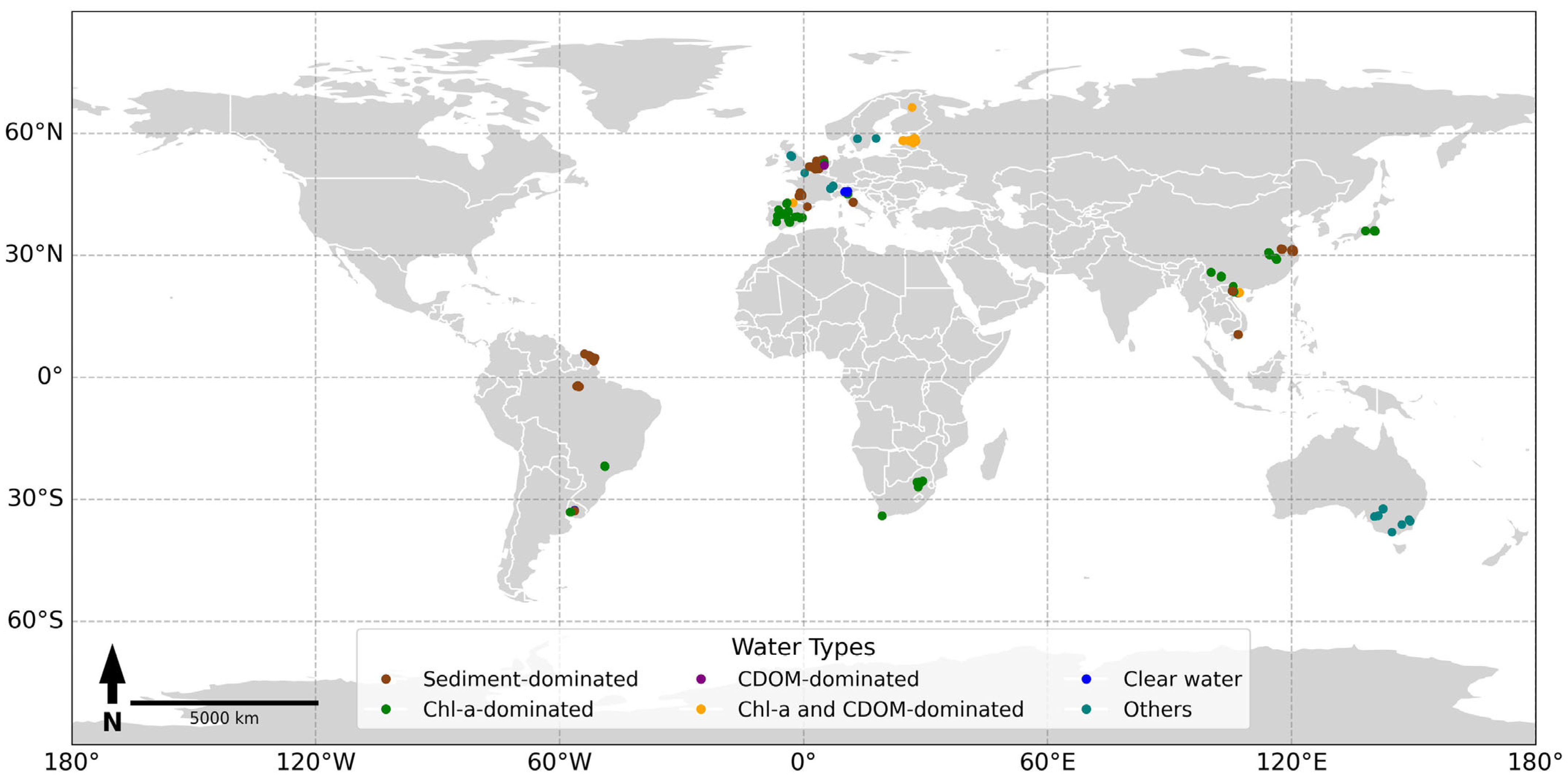
Therefore, the final dataset preparation merged convolved GLORIA Rrs and the corresponding combined turbidity measurements with the Sentinel-2 MAGEST Rrs and the corresponding in situ turbidity measurements. Quality screening removed observations with missing values or extreme reflectances (Rrs < 0.001 or >0.1), yielding 1373 high-quality observation pairs spanning diverse aquatic environments, i.e., lakes (55%), rivers (24%), coastal oceans (18%), and estuaries (2.5%) across 17 countries. Following GLORIA and MAGEST dataset, this final dataset represents sediment-dominated (61%), Chl-a-dominated (32.4%), colored dissolved organic matter (CDOM)-dominated (0.4%), both Chl-a and CDOM-dominated (3.5%), clear waters (0.5%), and other water types (2.2%) (Figure 2 and Figure A2,

Table A1. Data used for model training and performance evaluation to support the findings of this study.

Country	Site Name	Water Body Type	Water Type	No. of Samples	Turbidity Range (FNU)
Australia
Australia	Burrinjuck Dam	Lake	Others	1	11.49–11.49
Australia	Lake Burley Griffin	Lake	Others	2	10.23–13.67
Australia	Lake Hume	Lake	Others	1	21.92–21.92
Australia	Lake Pamamaroo	Lake	Others	7	102.56–151.02
Australia	Lake Victoria	Lake	Others	2	17.49–22.85
Australia	Wachtels Lagoon	Lake	Others	3	32.40–36.76
Australia	Western Treatment Plant	Others	Others	1	51.52–51.52
Belgium
Belgium	English Channel	Coastal ocean	Sediment-dominated	12	4.58–46.74
Brazil
Brazil	Curuai Lake	Lake	Sediment-dominated	14	3.92–37.90
Brazil	Ibitinga Reservoir	Lake	Chl-a-dominated	15	3.23–50.60
China
China	Chaohu	Lake	Sediment-dominated	40	12.52–339.40
China	Dianchi	Lake	Chl-a-dominated	63	19.84–158.76
China	Erhai	Lake	Chl-a-dominated	3	6.00–8.30
China	Hou Lake	Lake	Chl-a-dominated	22	18.40–102.50
China	Liangzi Lake	Lake	Chl-a-dominated	33	9.14–108.00
China	Poyang Lake	Lake	Chl-a-dominated	12	7.18–30.60
China	Taihu	Lake	Sediment-dominated	165	1.89–212.09
China	Wuhan East Lake	Lake	Chl-a-dominated	20	3.13–37.55
Estonia
Estonia	Lake Holstre	Lake	Chl-a and CDOM-dominated	1	9.73–9.73
Estonia	Lake Kaiavere	Lake	Chl-a and CDOM-dominated	1	9.66–9.66
Estonia	Lake Kooraste Linajarv	Lake	Chl-a and CDOM-dominated	1	16.65–16.65
Estonia	Lake Nohipalu Valgjarv	Lake	Chl-a and CDOM-dominated	1	2.20–2.20
Estonia	Lake Pangodi	Lake	Chl-a and CDOM-dominated	1	4.07–4.07
Estonia	Lake Peipsi	Lake	Chl-a and CDOM-dominated	21	1.13–22.85
Estonia	Lake Rouge Suurjarv	Lake	Chl-a and CDOM-dominated	2	2.57–3.92
Estonia	Lake Vortsjarv	Lake	Chl-a and CDOM-dominated	7	11.09–17.69
Estonia	Parnu Bay	Estuary	Chl-a and CDOM-dominated	4	12.87–17.34
Finland
Finland	Lake Vanttausjarvi	Lake	Chl-a and CDOM-dominated	1	2.37–2.37
France
France	Arcachon Bay	Coastal ocean	Sediment-dominated	17	1.64–1562.04
France	Arcachon Bay	Coastal ocean	Others	1	1.42–1.42
France	English Channel	Coastal ocean	Others	1	0.84–0.84
France	Gironde River	Estuary	Sediment-dominated	31	7.48–2124.59
France	Gironde River	River	Sediment-dominated	296	21.70–1953.84
France	Guiana	Coastal ocean	Sediment-dominated	126	2.70–1673.86
France	Guiana	Coastal ocean	Others	2	30.12–32.21
France	Guiana	Coastal ocean	Others	2	32.31–69.19
France	Guiana	Coastal ocean	Chl-a-dominated	7	10.28–258.20
Italy
Italy	Garda	Lake	Clear water	2	0.57–5.00
Italy	Iseo	Lake	Clear water	4	2.04–3.49
Italy	Mantova	Lake	Chl-a-dominated	15	4.97–15.11
Italy	Trasimeno	Lake	Sediment-dominated	7	3.92–24.57
Japan
Japan	Lake Kasumigaura	Lake	Chl-a-dominated	84	8.87–42.67
Japan	Shirakaba	Lake	Chl-a-dominated	1	8.28–8.28
Japan	Suwa	Lake	Chl-a-dominated	3	7.56–8.75
Netherlands
Netherlands (the)	English Channel	Coastal ocean	Sediment-dominated	12	1.92–58.40
Netherlands (the)	Ijsselmeer De Oude Zeug	Lake	Chl-a-dominated	1	21.07–21.07
Netherlands (the)	Loosdtrechtse plassen nr5	Lake	CDOM-dominated	1	14.68–14.68
Netherlands (the)	North Sea	Coastal ocean	Sediment-dominated	24	1.45–21.09
South Africa
South Africa	Bronkhorstspruit	Lake	Chl-a-dominated	4	7.02–11.66
South Africa	Hartbeespoort	Lake	Chl-a-dominated	11	4.78–2179.62
South Africa	Loskop	Lake	Chl-a-dominated	8	15.02–23.62
South Africa	Roodeplaat	Lake	Chl-a-dominated	9	3.92–50.80
South Africa	Theewaterskloof	Lake	Chl-a-dominated	10	8.90–25.53
South Africa	Vaal	Lake	Chl-a-dominated	5	4.61–72.74
Spain
Spain	Aguilar	Lake	Chl-a-dominated	1	8.54–8.54
Spain	Alarcón	Lake	Chl-a-dominated	1	5.57–5.57
Spain	Albufera	Lake	Chl-a-dominated	19	26.91–93.45
Spain	Alcántara	Lake	Chl-a-dominated	6	4.22–18.06
Spain	Almendra	Lake	Chl-a-dominated	1	4.80–4.80
Spain	Brovales	Lake	Chl-a-dominated	1	14.37–14.37
Spain	Contreras	Lake	Chl-a-dominated	1	3.88–3.88
Spain	Cortes	Lake	Chl-a-dominated	1	2.19–2.19
Spain	Ebro	Lake	Chl-a-dominated	3	4.94–17.46
Spain	Giribaile	Lake	Chl-a-dominated	1	3.86–3.86
Spain	Guadalén	Lake	Chl-a-dominated	1	8.71–8.71
Spain	Navalcán	Lake	Chl-a-dominated	3	12.54–18.17
Spain	Pinilla	Lake	Chl-a-dominated	3	4.44–8.15
Spain	Rosarito	Lake	Chl-a-dominated	30	1.82–25.39
Spain	Santa Teresa	Lake	Chl-a-dominated	1	3.85–3.85
Spain	Santillana	Lake	Chl-a-dominated	1	8.98–8.98
Spain	Terradets	Lake	Sediment-dominated	2	10.47–29.56
Spain	Ullívarri	Lake	Chl-a and CDOM-dominated	1	1.90–1.90
Spain	Valuengo	Lake	Chl-a-dominated	2	12.37–20.70
Spain	Vega de Jabalón	Lake	Chl-a-dominated	1	13.92–13.92
Sweden
Sweden	Baltic Sea	Coastal ocean	Others	1	1.06–1.06
Sweden	Lake Vänern	Lake	Others	2	1.25–1.29
Sweden	Lake Vanern	Lake	Chl-a-dominated	1	2.31–2.31
Switzerland
Switzerland	Lake Biel	Lake	Others	3	2.19–2.95
Switzerland	Lake Geneva	Lake	Others	3	0.74–2.89
United Kingdom
United Kingdom of Great Britain and Northern Ireland (the)	Bassenthwaite Lake	Lake	Others	1	1.49–1.49
United Kingdom of Great Britain and Northern Ireland (the)	English Channel	Coastal ocean	Sediment-dominated	9	1.74–102.27
United Kingdom of Great Britain and Northern Ireland (the)	Windermere	Lake	Others	2	1.98–5.51
Uruguay
Uruguay	Embalse de Paso del Palmar	Lake	Chl-a-dominated	24	12.70–100.00
Uruguay	Embalse de Paso del Palmar	Lake	Sediment-dominated	9	12.20–19.00
Uruguay	Lago Rincon del Bonete	Lake	Sediment-dominated	10	1.90–15.00
Uruguay	Lago Rincon del Bonete	Lake	Clear water	1	14.20–14.20
Viet Nam
Viet Nam	Ba Be Lake	Lake	Chl-a-dominated	2	13.38–15.19
Viet Nam	Gulf of Tonkin	Coastal ocean	Sediment-dominated	23	21.71–127.52
Viet Nam	Ha Long Bay, Quang Ninh Province	Coastal ocean	Chl-a and CDOM-dominated	7	12.01–14.29
Viet Nam	Red River	River	Sediment-dominated	34	36.95–115.40
Viet Nam	Soai Rap River	Coastal ocean	Sediment-dominated	6	35.97–207.05
Viet Nam	West Lake, Hanoi	Lake	Chl-a-dominated	15	20.95–70.37

).

2.4. Machine Learning Framework

2.4.1. Algorithm Selection and Configuration

Four regression algorithms were evaluated: Elastic Net (ENR), Random Forest (RFR), Gradient Boosting (GBR), and Extreme Gradient Boosting (XGBR). These span from linear (ENR) to complex ensemble methods, providing a comprehensive performance assessment. ENR [37] combines Ridge [38] and Lasso [39] regressions to handle multicollinearity while performing feature selection. It is quite flexible, allowing tuning between both models, enabling shrinkage and selection of correlated feature groups. RFR, an ensemble method, aggregates multiple decision trees for robust nonlinear modeling with minimal tuning requirements [40]. However, it may be biased toward dominant feature groups and can be slow to train. GBR is another ensemble method that sequentially builds trees to correct predecessor errors, offering high accuracy through iterative refinement [41]. It is flexible and often accurate but sensitive to noise, slower to train, and more tuning-intensive than RFR. XGBR extends GBR with regularization and computational optimizations for enhanced efficiency [42].

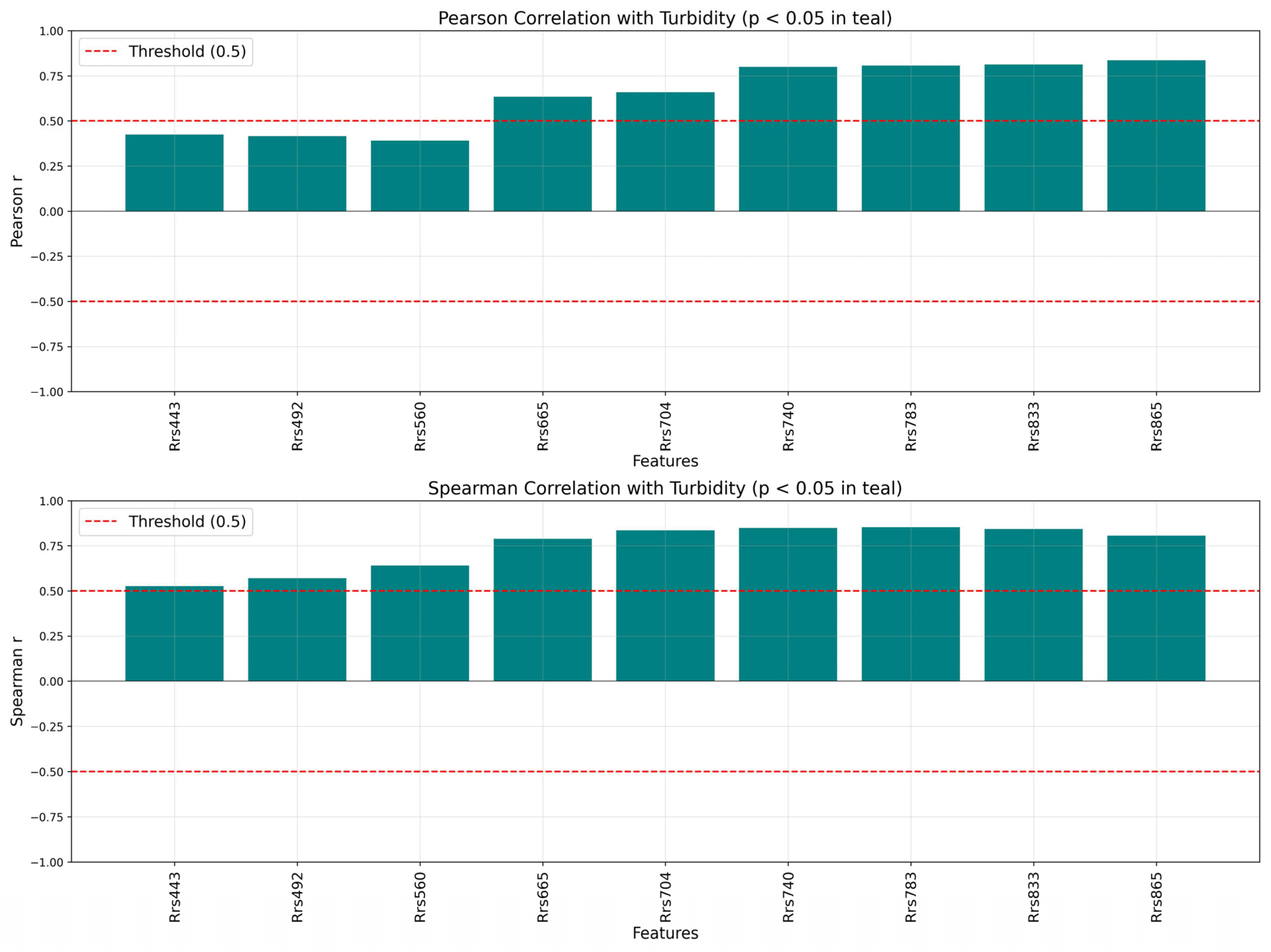
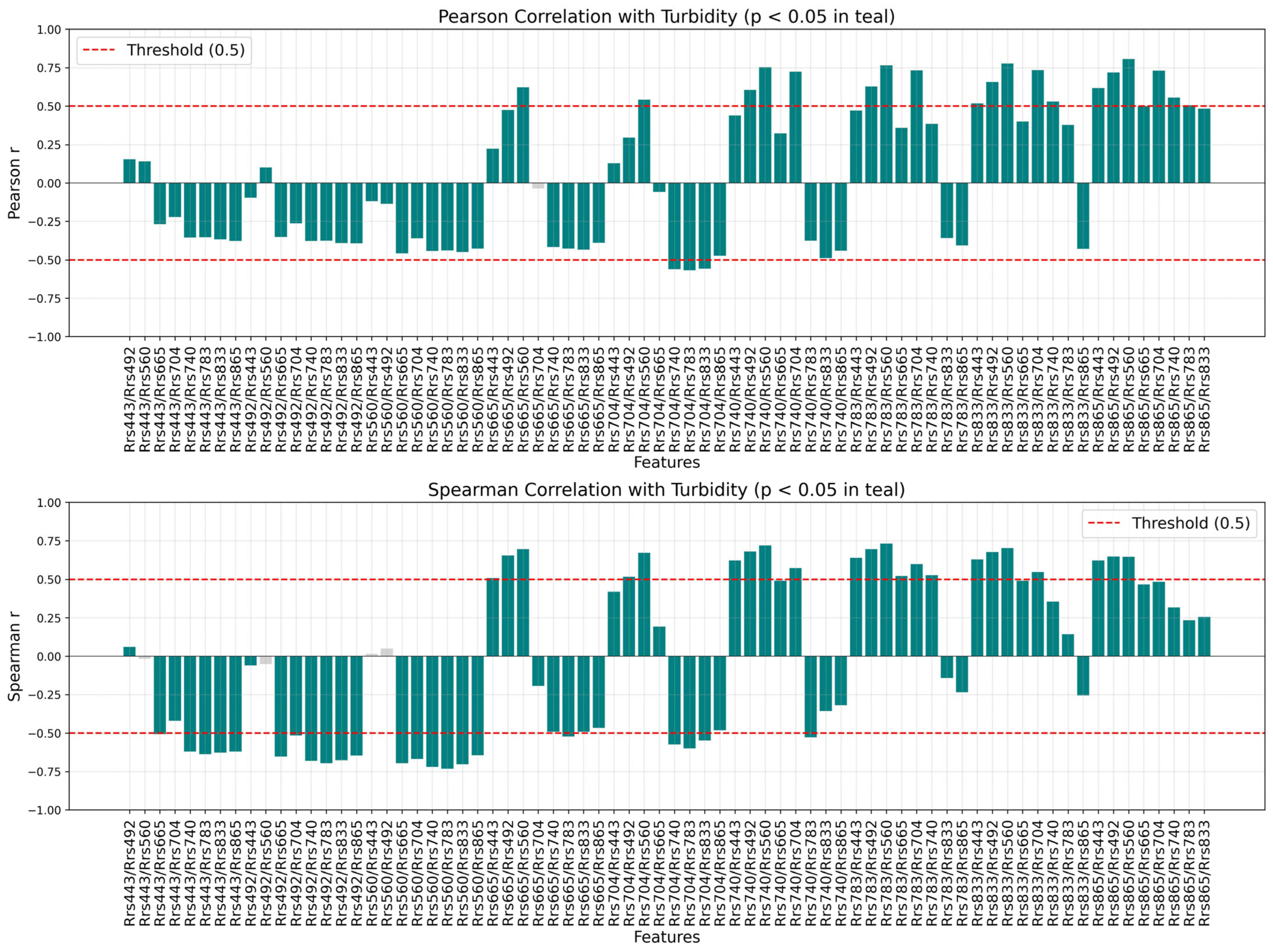
Input feature comprised all nine Sentinel-2 visible and near-infrared (VNIR) bands (443–865 nm) to leverage the full spectral information available for turbidity characterization. This comprehensive approach allowed the model to capture subtle spectral variations across different water types and turbidity ranges, as turbidity affects reflectance differently across the VNIR spectrum [17]. The Rrs865/Rrs560 ratio was included as an additional feature based on its strong correlation with turbidity (r = 0.81) among all the tested spectral ratios during the exploratory analysis (Figure A3 and Figure A4). All features underwent min-max normalization to the [0,1] range, ensuring comparable scales and preventing bias toward high-magnitude features during model training. Turbidity values were mean-centered to enhance model sensitivity to relative variations rather than absolute magnitudes.

Data partitioning employed a 75:25 train–test split using a fixed random state (random state = 42) to ensure reproducibility across experiments. This approach randomly assigned observations to training (75%, n = 1029) or testing (25%, n = 344) datasets while maintaining the overall turbidity distribution. In addition, this fixed random state eliminated variability between model runs, enabling consistent performance comparisons across different algorithms and hyperparameter configurations.

To minimize overfitting and ensure robust hyperparameter selection, 5-fold cross-validation was implemented during training. This approach evaluated model performance across five independent data splits within the training set, with each fold serving as validation once, while the remaining four provided training data. Cross-validation provides more reliable performance estimation than single train-validation splits by averaging results across multiple data configurations, reducing the influence of any particular data partition [43]. Hyperparameters were optimized through grid search across the cross-validation folds, tuning tree count, maximum depth, learning rate, and regularization parameters for ensemble models; alpha and L1-ratio for ENR.

2.4.2. Model Evaluation and Interpretability

After training, the model’s performance was assessed on the unseen test dataset and on an independent dataset from the Albufera Lake, Valencia, Spain (2023–2025) [44], with predictions reconstructed by adding the training mean to the model outputs. To provide a comprehensive analysis, the trained models were compared against two established empirical models from Table 1 [13,17] using the identical test dataset. Comparative performance of the six models was assessed using RMSE, r, mean absolute error (MAE), and bias.

Model interpretability employed SHAP analysis to quantify feature contributions through Shapley values derived from cooperative game theory [30,45]. SHAP decomposes each prediction into additive feature contributions, providing both global feature importance rankings and local explanations for individual predictions. Summary plots visualized feature importance with directional effects, while dependence plots revealed nonlinear relationships between features and turbidity across different optical regimes. Pairwise interaction effects among the most influential features generated unique visualizations, identifying synergistic or antagonistic relationships critical for understanding the model behavior. Decision plots illustrated cumulative feature contributions along prediction paths, revealing the model’s internal logic from baseline to final prediction.

2.4.3. Uncertainty Quantification

The comprehensive uncertainty analysis quantified prediction reliability across the turbidity spectrum. The residual analysis examined the prediction errors (differences between observed and predicted turbidity) to identify systematic biases and heteroscedasticity patterns [46,47]. The confidence intervals (CI) for the regression line and prediction intervals (PI) for individual observations were computed following standard regression theory [48,49].

The 95% CI, representing uncertainty in the mean prediction, was computed as:

$$\mathrm{CI}=\mathsf{ӯ}\pm {\mathrm{t}}_{0.025,\mathrm{n}-2}\times {\sigma }_{\mathrm{res}}\times \surd (1/\mathrm{n}+{(\mathrm{x}-\bar{\mathrm{x}})}^2/\Sigma {(\mathrm{x}i-\bar{\mathrm{x}})}^2)$$

(3)

where ӯ represents the predicted value, σ_res is the residual standard error, n is the sample size, x is the prediction point, $\bar{\mathrm{x}}$ is the mean of observations, and t_0.025,n−2 is the critical t-value at 95% confidence with n − 2 degrees of freedom.

The 95% PI, capturing uncertainty for individual predictions including natural variability, incorporated an additional unit term:

$$\mathrm{PI}=\mathsf{ӯ}\pm {\mathrm{t}}_{0.025,\mathrm{n}-2}\times {\sigma }_{\mathrm{res}}\times \surd (1+1/\mathrm{n}+{(\mathrm{x}-\bar{\mathrm{x}})}^2/\Sigma {(\mathrm{x}i-\bar{\mathrm{x}})}^2)$$

(4)

These intervals provided operational guidance for end-users, with CI indicating the reliability of the regression line (mean predictions) and PI bounding the range within which 95% of the individual observations are expected to fall [48,50].

2.5. Automated Processing Pipelines

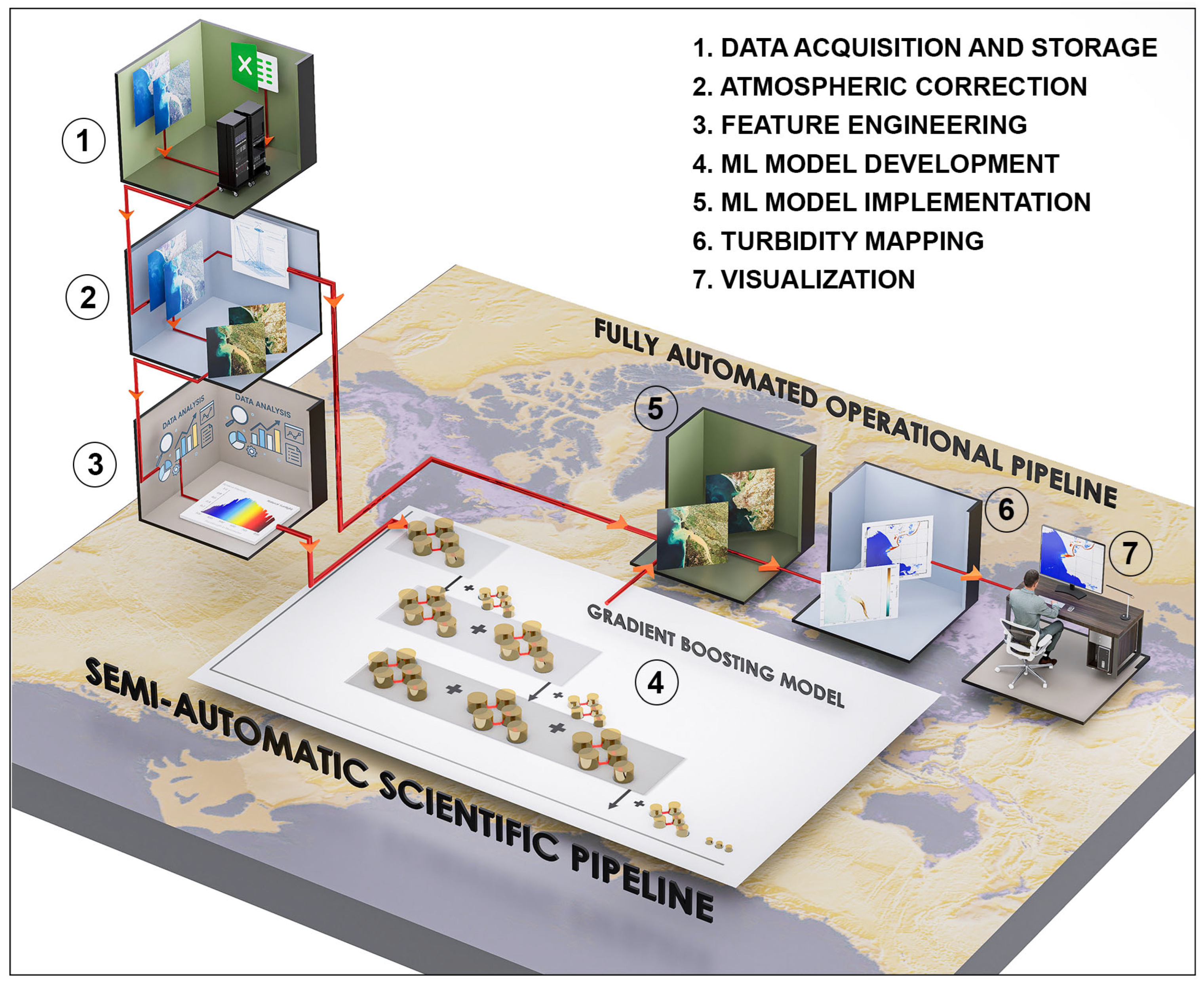
Two processing pipelines were developed to support both algorithm development and operational deployment: a semi-automated scientific pipeline for scientific experimentation, model development, and validation, and a fully automated operational pipeline for routine turbidity monitoring (Figure 3). Both pipelines were implemented within the scientific exploitation platform (SEP) under the SIMBAD (Sentinel Imagery Multiband Analysis and Dissemination) project (https://simbad.quasarsr.com/) (accessed on 7 November 2025), designed for Earth observation data processing in distributed computing environments [51].

The pipelines utilize Docker containerization to ensure consistent execution across different computing environments by bundling application code, dependencies, and runtime configurations into portable containers. Kubernetes orchestration manages computational resources and enables parallel processing through dynamic workload distribution across available nodes. Data storage and accessibility within SEP are handled by a centralized Network File System, facilitating seamless data access across the distributed infrastructure. Pipeline configurations are externalized into environment-specific files, allowing modification of processing parameters (e.g., file paths, satellite identifiers, temporal windows, etc.) without code changes.

The semi-automated scientific pipeline supports iterative model development through modular components for satellite data download, atmospheric correction and matchup extraction, feature engineering and data preprocessing, model training with cross-validation, and model implementation, validation, performance evaluation and visualization. Manual intervention points allow quality control and parameter adjustment during the model development phases. In contrast, the operational pipeline automates end-to-end processing for routine monitoring: downloading Sentinel-2 imagery, applying atmospheric corrections, executing the pre-trained model, and generating georeferenced turbidity products in GeoTIFF format. The modular architecture facilitates maintenance and updates, while containerization and Kubernetes orchestration ensure reproducibility across parallel deployments.

3. Results

3.1. Model’s Performance Evaluation

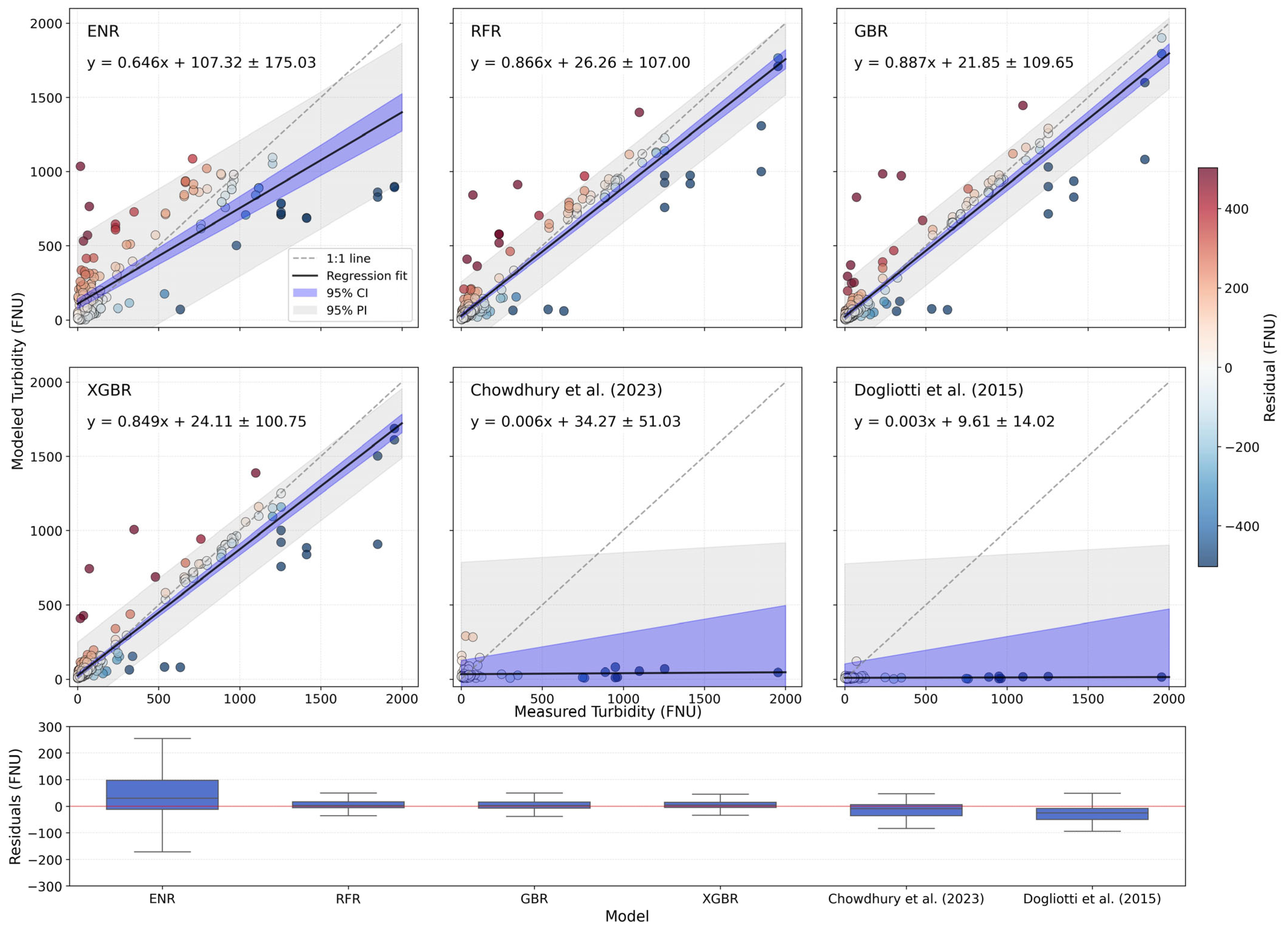
The comprehensive analysis of six turbidity prediction models on the test dataset (n = 344) revealed distinct performance characteristics, as evidenced by both the regression analysis and comprehensive statistical metrics (

Table 3. Performance metrics for turbidity models on test dataset (n = 344).

Model	r	R2	RMSE (FNU)	MAE (FNU)	Bias (FNU)
ENR	0.83	0.69	226.56	127.11	21.19
RFR	0.95	0.89	117.12	47.10	1.86
GBR	0.95	0.90	116.62	43.24	1.32
XGBR	0.95	0.90	114.21	41.56	−3.29
Chowdhury et al., 2023 [17]	0.05	−0.13	369.92	152.61	−123.81
Dogliotti et al., 2015 [13]	0.06	−0.18	377.29	151.79	−149.11

and Figure 4). The four ML models (ENR, RFR, GBR, and XGBR) demonstrated substantially better performance compared to the two empirical algorithms, with the ensemble methods (RFR, GBR, and XGBR) achieving r-values of 0.95 and R² values of 0.89–0.90, indicating that these models explain approximately 90% of the measured turbidity variance. Among these, GBR emerged as the optimal model, combining the highest slope (0.887)—the closest to the ideal value of 1.0, the lowest bias (1.32 FNU), and the second-best MAE (43.24 FNU), demonstrating both accuracy and precision across the entire measurement range.

The GBR model’s performance was further validated by its comprehensive statistical metrics. With an R² value of 0.90 and RMSE of 116.62 FNU, GBR demonstrated robust predictive capability while maintaining minimal systematic error. The remarkably low bias of 1.32 FNU indicated that the model’s predictions are nearly unbiased on average, a critical characteristic for operational water quality monitoring. While XGBR showed marginally better RMSE (114.21 FNU) and MAE (41.56 FNU) values, its negative bias (−3.29 FNU) and lower slope (0.849) suggested a tendency toward systematic underestimation, which is particularly problematic for high turbidity detection. RFR, despite sharing the same correlation coefficient (0.95) and similar R² (0.89), exhibited slightly higher errors (RMSE: 117.12 FNU, MAE: 47.10 FNU) and a lower slope (0.886) compared to GBR, confirming GBR’s superiority in balancing multiple performance criteria. ENR, while demonstrating reasonable correlation (r = 0.83, R² = 0.69), showed substantially higher error metrics with an RMSE of 226.56 FNU and MAE of 127.11 FNU. The model’s slope of 0.646 indicated systematic underestimation by approximately 35%, and despite a moderate bias of 21.19 FNU, the large standard error (±175.03 FNU) limited its utility for precise turbidity quantification.

The empirical algorithms revealed fundamental limitations. Both models demonstrated severe underestimation, with near-zero correlation coefficients (0.05 and 0.06) and negative R² values (−0.13 and −0.18). The extreme negative biases (−123.81 and −149.11 FNU) and high error metrics (RMSE > 369 FNU, and MAE > 151 FNU) confirmed severe systematic underestimation when applied to the same test dataset. The models’ near-zero slopes (0.006 and 0.003) indicated a lack of sensitivity to turbidity variations, with predictions remaining clustered below 500 FNU regardless of the actual turbidity levels exceeding 2000 FNU.

In addition, the uncertainty analysis provided essential insights into model reliability and uncertainty quantification that extended beyond simple error metrics. While CI represented uncertainty in the mean prediction (the regression line itself), the PI captured the total prediction uncertainty, including model variance and measurement noise. The 95% PI represented the range within which 95% of future observations are expected to fall, given the model’s inherent uncertainty. Though both GBR and XGBR showed similar PI and CI width, unlike XGBR, the 1:1 line fell entirely within GBR’s 95% PI across the full turbidity range, indicating that the model is well calibrated and the uncertainty estimates are statistically consistent, which means users can trust that these uncertainty bounds are neither overly optimistic nor unnecessarily conservative. The residual distribution analysis also showed that GBR maintained consistent prediction variance across turbidity ranges, whereas XGBR exhibited heteroscedastic behavior with increasing underestimation at high turbidity levels (>1000 FNU). Based on this comprehensive evaluation, GBR was selected as the optimal model for operational turbidity monitoring.

3.2. Model Interpretation

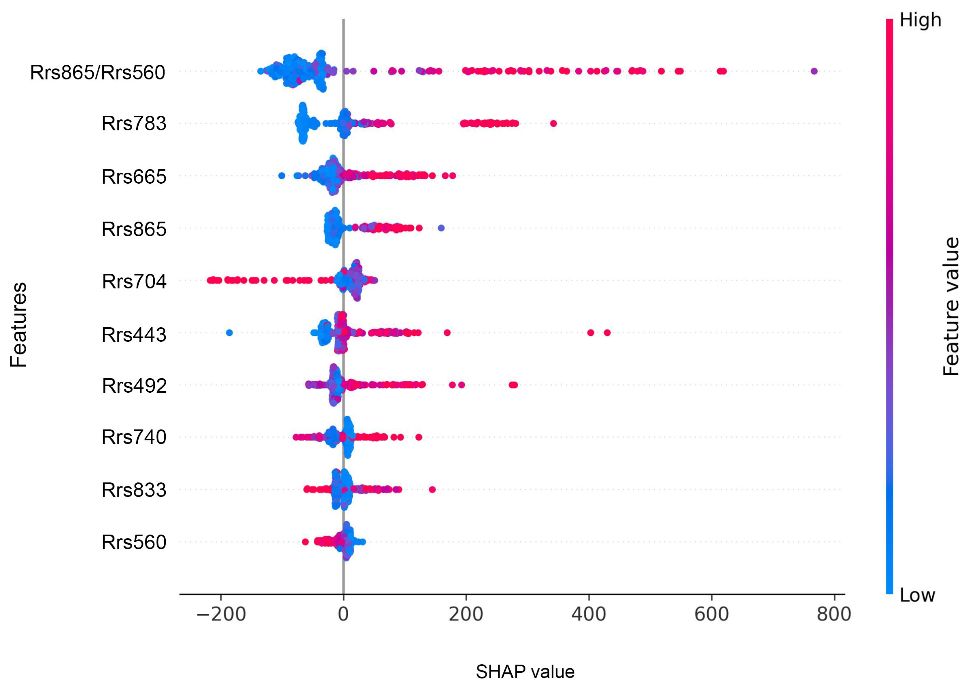
SHAP analysis revealed the physical basis underlying GBR predictions by quantifying feature contributions across the turbidity range. The Rrs865/Rrs560 ratio emerged as the dominant predictor, with SHAP values extending up to 800 units, exceeding all other features (Figure 5). This ratio, comparing NIR backscattering (865 nm) to visible reflectance (560 nm), effectively discriminated turbidity through its sensitivity to particle-induced spectral changes. Low ratio values (blue points) consistently produced negative SHAP contributions, suppressing turbidity predictions, while high values (pink points) generated strong positive contributions, amplifying predictions.

Individual bands showed hierarchical importance, with Rrs783, Rrs665, and Rrs865 providing the next tier of contributions (Figure 5). These red and NIR bands, sensitive to suspended sediment backscattering, showed clear positive relationships—higher reflectance values (pink) increased the predicted turbidity while lower values (blue) decreased it. The remaining features (Rrs443, Rrs492, Rrs740, Rrs833, and Rrs560) contributed minimally, with SHAP values clustering near zero, suggesting they provided minor refinements rather than primary predictive power.

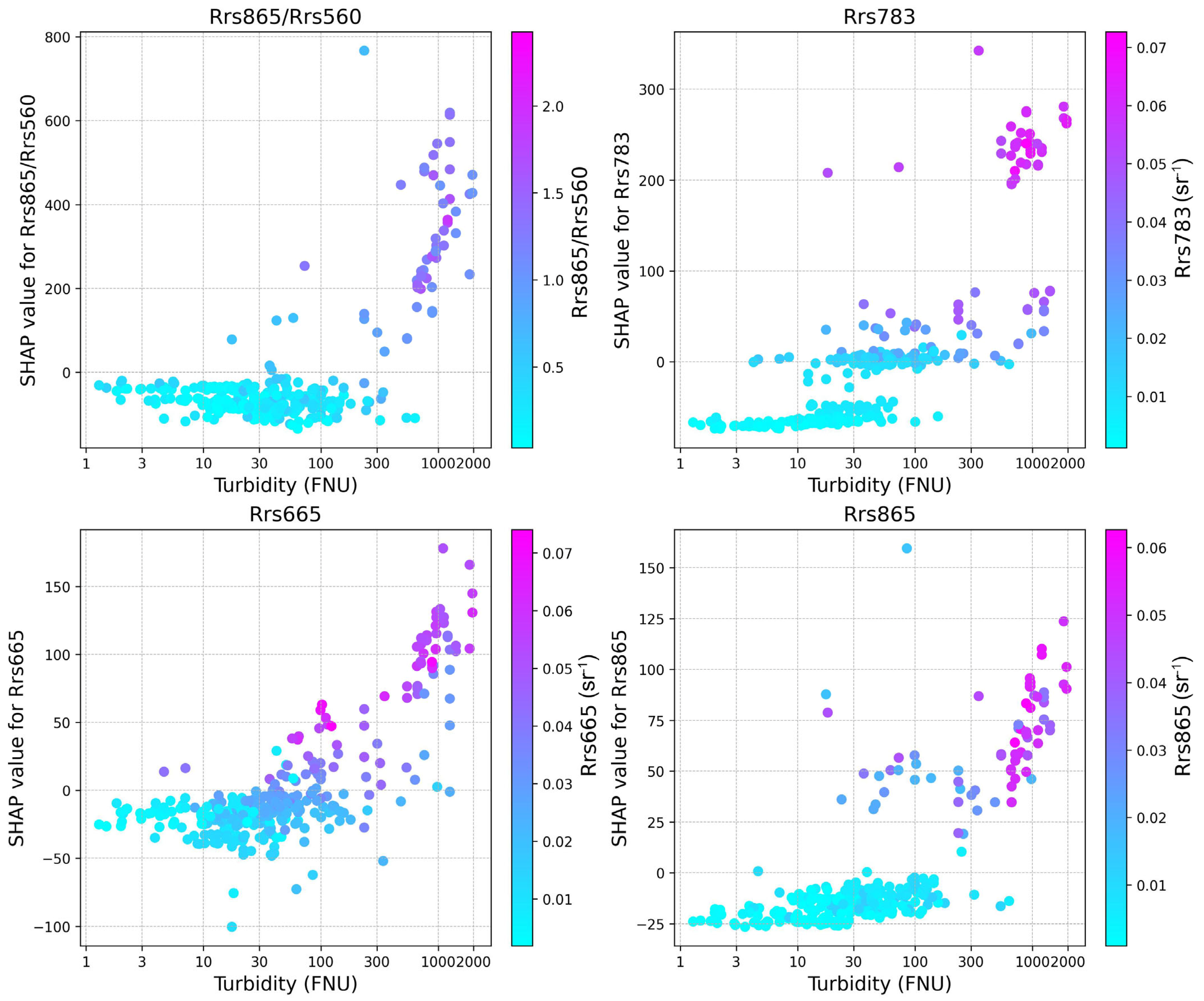
Examining SHAP values across the turbidity spectrum revealed distinct threshold behaviors and saturation patterns (Figure 6). The Rrs865/Rrs560 ratio exhibited a sharp nonlinear response: SHAP values remained near zero for turbidity below 30 FNU and ratio values below 0.75, then increased dramatically as the ratio exceeded 1.0, particularly between 100–1000 FNU. This threshold at the ratio ≈ 1.0 represents a physical transition where NIR backscattering begins to dominate over visible reflectance, signaling high particle concentrations. The contribution plateaued around 1500 FNU, suggesting saturation in the model’s reliance on this feature.

Rrs783 showed a similar but less pronounced pattern, with SHAP values remaining minimal below 30 FNU, then increasing steadily between 30–500 FNU before plateauing. Rrs665 demonstrated relatively linear behavior up to 500 FNU before saturating beyond ~750 FNU. In high turbid waters, the reflectance in Rrs665 often reaches an optical maximum, where additional suspended sediments do not further increase reflectance due to multiple scattering and absorption [17]. The model appears to have internalized this physical behavior, reducing the marginal weight of Rrs665 in the upper turbidity range.

Rrs865 provided gradual, consistent contributions across the entire range without sharp thresholds or clear saturation (Figure 6). This suggested that while Rrs865 was not the primary trigger for high turbidity predictions, it provided steady contextual information that reinforced trends identified by other features. Unlike Rrs865/Rrs560 or Rrs665, it did not dominate the model’s output in any specific regime. Instead, it appeared to function as a stabilizing feature, contributing modestly but consistently to turbidity prediction across the measurement range.

The SHAP interaction plots revealed how secondary features modulated the primary features’ contributions to turbidity predictions (Figure 7). The Rrs865/Rrs560 ratio showed consistent threshold behavior across all interactions (top row). When Rrs865/Rrs560 values remained below 0.5, SHAP contributions clustered near zero regardless of secondary feature values. However, once the ratio exceeded 1.0, SHAP values increased dramatically to 400–800 units, with the steepest increase occurring between ratios of 1.0–1.5. Furthermore, the threshold effects of Rrs865/Rrs560 reinforced when Rrs783, Rrs665, and Rrs865 reflectance values were also elevated, revealing a synergistic pattern, where multiple indicators of particle scattering aligned, strengthening the model’s output. In contrast, the interactions between Rrs783 and Rrs665 were more additive and linear, suggesting that the model relied on both reflectance values independently to characterize turbidity. Notably, the SHAP contribution of Rrs665 saturated at high reflectance, which the model appeared to account for by tapering its influence in highly turbid waters.

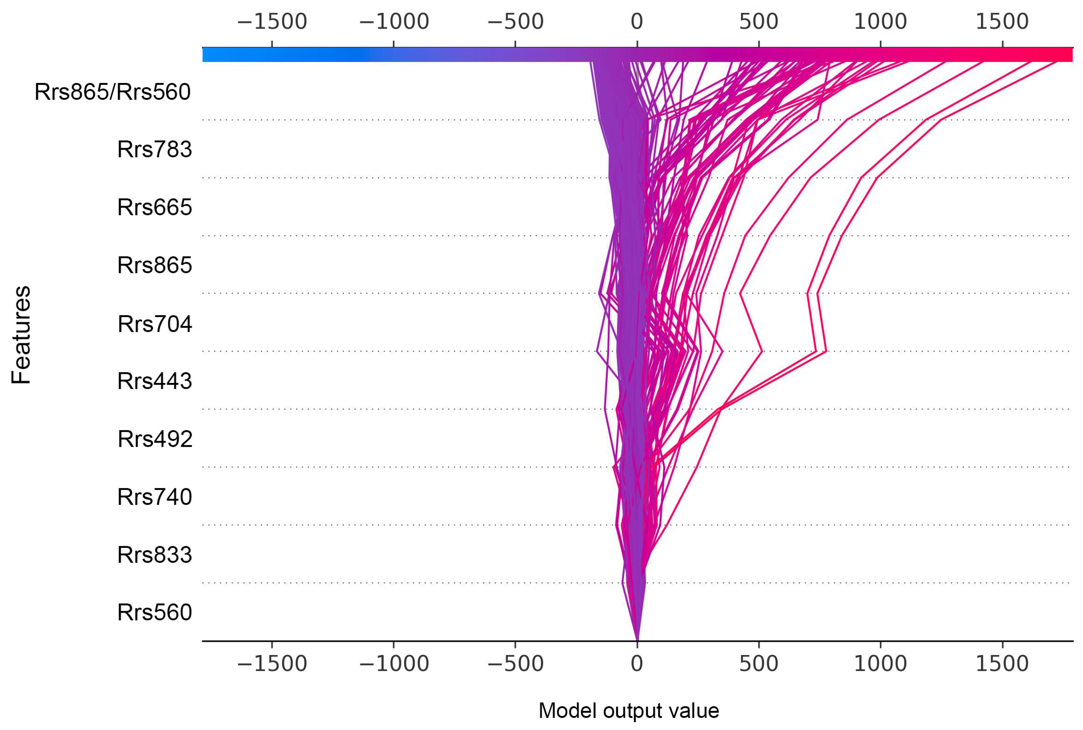
Finally, the SHAP decision plot illustrated how the model sequentially accumulated evidence from individual features to reach final turbidity predictions (Figure 8). The x-axis at the top shows cumulative SHAP values that track the running sum of feature contributions, while the bottom x-axis displays the final model output values after adding these contributions to the baseline. Each line represents a single prediction’s path, starting from the baseline (0, representing mean training turbidity) and sequentially incorporating feature contributions as the path moves upward through the feature stack.

The plot revealed distinct prediction regimes. For example, low turbidity predictions (0–100 FNU) remained tightly clustered near zero, with minimal deviation even after incorporating all features. These paths showed that the low Rrs865/Rrs560 ratio values immediately pulled predictions leftward by −300 SHAP units, and subsequent features made only minor adjustments, keeping final predictions below 100 FNU. Moderate turbidity predictions between 100–1000 FNU showed gradual divergence from the baseline. The Rrs865/Rrs560 ratio provided positive contributions of SHAP units, followed by incremental additions from Rrs783 and Rrs665. These paths exhibited more variation as they progressed through the feature stack, reflecting the model’s integration of multiple spectral signals to refine predictions within this intermediate range. At high turbidity, predictions (>1000 FNU) demonstrated dramatic rightward trajectories. The Rrs865/Rrs560 ratio alone often contributed to high SHAP units, immediately pushing predictions toward extreme values. Subsequent features (Rrs783 and Rrs665) provided secondary adjustments, while Rrs865 and Rrs704 offered minor refinements. The remaining features (Rrs443, Rrs492, Rrs740, Rrs833, and Rrs560) contributed negligibly, with paths showing no horizontal movement at these levels.

3.3. Model Performance Across Optical Water Types

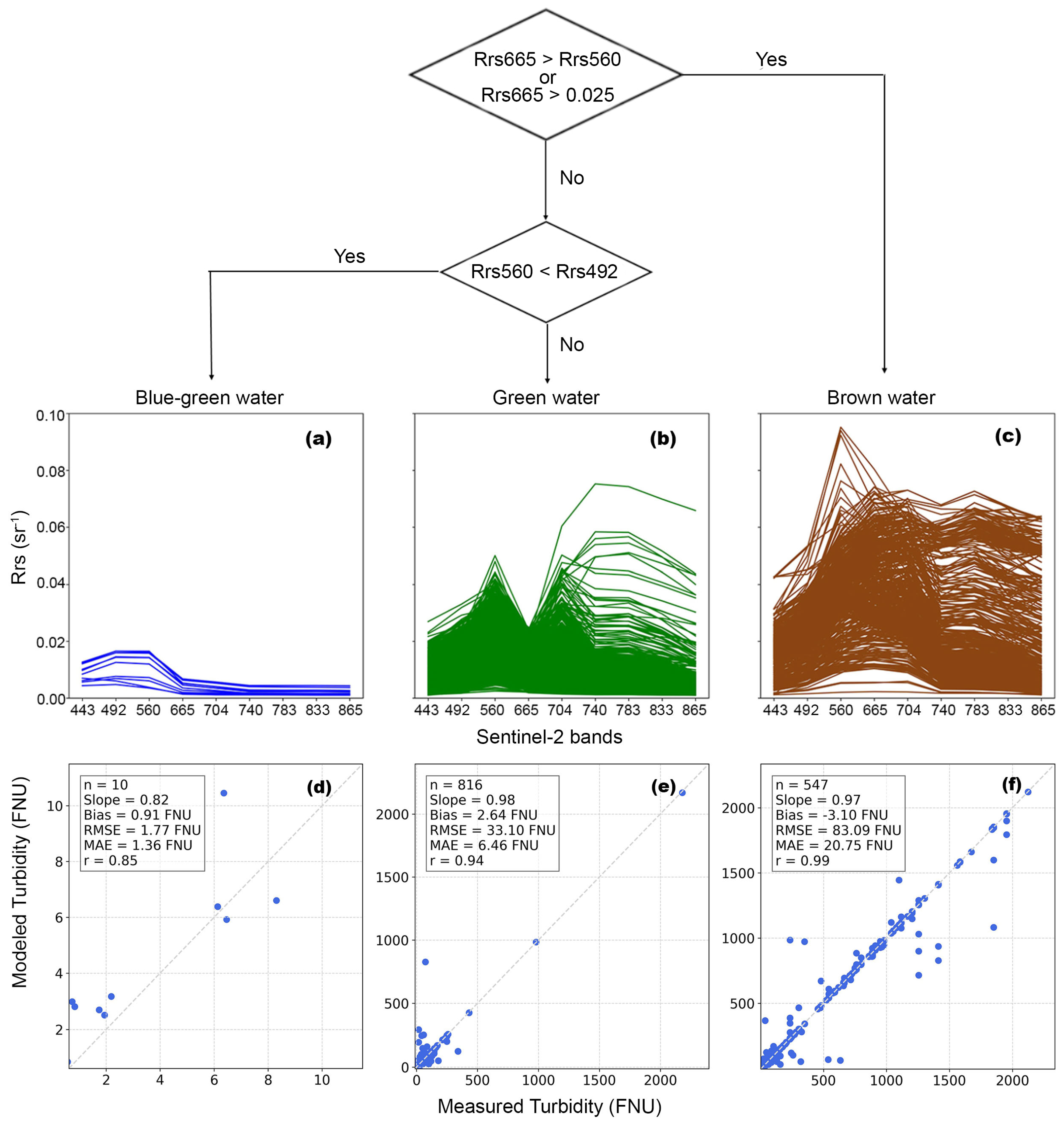
The GBR model maintained robust performance across optically distinct water types (Figure 9), classified following the established spectral criteria [31]. In this case, the combined dataset containing both training and test observations was first classified as brown waters when Rrs665 > Rrs560 or Rrs665 > 0.025. If neither condition was met, but Rrs560 < Rrs490, the water was categorized as blue-green waters. Otherwise, the water was classified as green water.

In oligotrophic blue-green waters (n = 10), the model achieved a strong correlation (r = 0.85) with minimal bias (0.91 FNU) and low errors (RMSE: 1.77 FNU, MAE: 1.36 FNU), though slight underestimation was observed (slope: 0.82). Green waters dominated by Chl-a and suspended matter (n = 816) showed excellent agreement (r: 0.94, slope: 0.98) with moderate errors (RMSE: 33.10 FNU, MAE: 6.46 FNU). Sediment-dominated brown waters (n = 547) demonstrated exceptional predictive accuracy (r: 0.99, slope: 0.97) despite the high absolute errors (RMSE = 83.09 FNU, MAE = 20.75 FNU), which are attributable to the wide turbidity range of up to 2200 FNU.

3.4. Model Application Across Diverse Geographic Settings

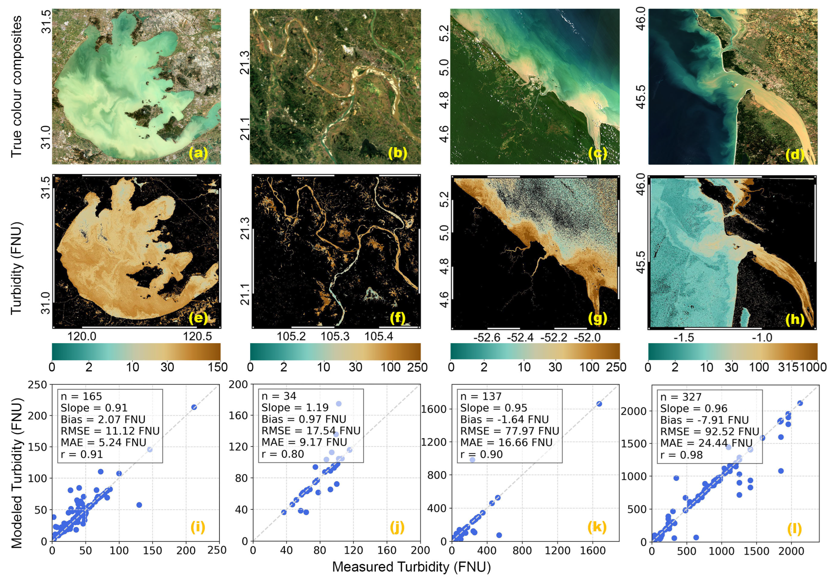
Model applications across four distinct aquatic systems demonstrated consistent performance independent of geographic location (Figure 10). Lake Taihu, China’s third-largest freshwater lake experiencing severe eutrophication and cyanobacterial blooms [52], showed strong agreement (r: 0.91) across turbidity ranges from 0 to 250 FNU using data from 2008–2011. The model’s application on the Red River (Vietnam), a major sediment-laden river system with an annual suspended sediment flux exceeding 100 million tons [53], exhibited a correlation of 0.80 for similar turbidity ranges (0 to 250 FNU) using field measurements from the year of 2017.

Coastal waters of French Guiana (North Atlantic coast), characterized by extensive Amazon River sediment plumes and complex optical properties from CDOM and suspended sediments [54], showed strong model performance (r: 0.9) despite these challenging conditions. The Gironde Estuary (France), Europe’s largest estuary with a well-documented maximum turbidity zone, where suspended sediment concentrations can exceed 1000 mg/L [55], maintained high correlation (r: 0.98) even for extreme turbidity values of up to 2000 FNU.

Turbidity maps generated for each system revealed characteristic spatial patterns consistent with documented hydrodynamic processes: wind-driven resuspension gradients in shallow Lake Taihu [56], downstream sediment transport patterns in the Red River delta, estuarine circulation in the Gironde Estuary [57], and northwest-flowing coastal plumes along French Guiana driven by the North Brazil Current [58]. These spatially coherent patterns, aligning with known regional oceanographic and limnological understanding, confirm the model’s ability to capture physical phenomena across diverse environmental settings.

3.5. Model Validation in an Independent Site

The independent validation results (Figure 11) demonstrated the GBR model’s exceptional generalization capability when applied to Albufera Lake, Spain. The model achieved noteworthy performance metrics with an RMSE of 19.39 FNU and an MAE of 15.29 FNU, representing an 83% reduction in RMSE compared to the test dataset (116.62 FNU). The high correlation (r = 0.81) and minimal bias (9.46 FNU) confirmed the model’s ability to accurately predict turbidity in this independent water body without site-specific calibration.

The uncertainty quantification analysis revealed a particularly robust model behavior at Albufera Lake. All validation samples (100% coverage) fell within the 95% prediction intervals established from the test dataset, indicating that the model’s uncertainty bounds remain reliable when extrapolated to new independent data. The RMSE ratio of 0.17 (validation/test) demonstrated that the model performed approximately six times better at Albufera than on the heterogeneous test dataset, likely due to the lake’s more homogeneous optical properties compared to the diverse water bodies in the training and test datasets. This performance improvement, rather than degradation, suggested that the model successfully learned generalizable relationships between spectral signatures and turbidity that transferred well to lacustrine environments.

3.6. Performance of Automated Pipelines

The dockerized workflows demonstrated operational readiness through sustained performance metrics (

Table 4. Average runtime per step for the operational turbidity monitoring system.

Processing Steps	Description	Avg. Runtime
Satellite data download	Fetching Sentinel-2 imagery from defined sources	~30–45 min/100 images
Atmospheric correction	DSF-based correction using ACOLITE	~10–45 min/image
Feature extraction, and model implementation	Preparing input feature variables, and applying the pre-trained model to produce turbidity maps	Few min to <1 h
Validation and diagnostics	Comparing predictions with observations, computing accuracy metrics, etc.	Few min/image
Output logging	Saving trained model, metadata, and logs	Few s/image

). For turbidity monitoring, the pipeline achieved near-real-time capability through several optimizations. Processing time from satellite overpass to product delivery consistently remained under 3 h, with a typical runtime of less than 3 min per Sentinel-2 tile, excluding atmospheric correction. Leveraging SEP’s Kubernetes parallel cluster processing capabilities, turbidity mapping across the entire Spanish–Portuguese coast (38 Sentinel-2 tiles) can be completed in under 3 min without atmospheric correction, and within 30 min to 1 h with atmospheric correction.

4. Discussion

In this study, a globally applicable turbidity monitoring system has been developed using a Gradient Boosting Regression (GBR) model. GBR is a data-driven machine-learning (ML) technique, capable of capturing complex optical signatures across diverse aquatic environments at 10 m spatial resolution. The model’s superior performance (r = 0.95, bias = 1.32 FNU) (Figure 4) across a 0–2200 FNU range substantially exceeded existing empirical algorithms [13,17], which failed at high turbidity levels with near-zero correlations and systematic underestimation. This performance gain stems from GBR’s capacity to learn nonlinear spectral-turbidity relationships through iterative error correction [41,59,60,61], rather than relying on predetermined mathematical functions that cannot accommodate global optical variability.

Typically, turbidity increases reflectance in the visible and near-infrared (VNIR) wavelengths, particularly in green (500–600 nm), red (600–700 nm), and NIR (~800 nm) bands [62,63,64,65,66]. However, its spectral responses vary with sediment composition, phytoplankton abundance, and dissolved organic matter [67]. The physical interpretability revealed through SHAP analysis (Figure 5, Figure 6, Figure 7 and Figure 8) demonstrated that the model has internalized these fundamental optical principles. The dominance of the Rrs865/Rrs560 ratio, with its sharp transition at the ratio ≈ 1.0 indicated the physical shift from absorption-dominated to scattering-dominated optical regimes as particle concentrations increase. Similarly, the model automatically accounts for the saturation of Rrs665 reflectance at high turbidity levels (a known optical limit where multiple scattering prevents further reflectance increases [17,65]), by reducing band weighting at extreme turbidity levels. This learned representation of optical physics provides confidence in the model’s extrapolation capabilities beyond its training domain.

The model’s validation at the Albufera Lake (Figure 11) and its performance across different optical water types, i.e., blue-green, green, and sediment-rich brown waters, as well as across different geographical settings (Figure 9 and Figure 10), demonstrated a consistently high predictive reliability. Although a slight underestimation in low-turbidity blue-green waters was observed, exceptional performance was achieved in sediment-dominated waters. The model’s performance from the eutrophic lakes Albufera [68] and Taihu [52] to the hyperturbid Gironde Estuary [55] confirmed that a single global model can capture site-specific hydrodynamic processes without regional tuning. The spatial representation of turbidity plumes (Figure 10 and Figure 11) indicated the model’s sensitivity to underlying physical drivers. While region-specific models might achieve marginally higher local accuracy through reduced complexity [26,69], the operational advantages of a unified global approach—consistency, interoperability, and simplified maintenance outweigh minor performance trade-offs.

The successful integration of heterogeneous datasets (GLORIA and MAGEST) through rigorous quality control and spectral harmonization addressed a fundamental challenge in the global algorithm development: the lack of consistent, quality-assured training data spanning diverse optical conditions. Though the proxy-derived GLORIA turbidity values (Table 2, Figure A1) introduced quantifiable uncertainty (i.e., 37–44% relative MAE), they enabled critical coverage of under-sampled environments. This pragmatic approach balanced data quality with representativeness, a trade-off inherent in transitioning from local to global monitoring capabilities.

Atmospheric correction remained another source of uncertainty, particularly in NIR bands (Figure 1), where ACOLITE’s performance degrades at high turbidity levels [35]. This uncertainty in Rrs783 and Rrs865 (key bands for the GBR model) within the MAGEST dataset propagated through turbidity estimates, suggesting that further improvements in atmospheric correction algorithms would yield improved accuracy. Future investigations should systematically compare existing correction processors across diverse atmospheric and aquatic conditions to quantify and potentially correct these uncertainties. Additionally, it is crucial to assess the impact of adjacency effects and bottom reflectance contributions, both of which are prevalent yet challenging to quantify accurately. These factors can significantly influence the retrieved water properties and, if not properly accounted for, may introduce biases in the analysis. A comprehensive evaluation of these elements in future analysis, i.e., evaluating and utilizing the RAdCor algorithm within the ACOLITE processor, will further enhance the reliability of remote sensing observation and improve the accuracy of the turbidity assessment.

The operational pipeline’s achievement—3 h processing time from satellite overpass to turbidity product—represents a critical advancement for environmental monitoring applications requiring timely information. The containerized architecture ensured reproducibility while enabling seamless integration of future improvements, including new training data, alternative sensors, or enhanced atmospheric correction algorithms. This technical infrastructure transformed the algorithm from a research tool to an operational capability suitable for routine monitoring programs [44].

However, data limitations at extreme turbidity ranges highlight priorities for future development. The underrepresentation of oligotrophic waters (n = 10) (Figure 9) explains the observed underestimation in clear conditions, while sparse sampling above 1500 FNU limits confidence in hyperturbid environments (Figure 4). Recognizing that data sparsity, particularly at extreme turbidity levels, poses a significant challenge, alternative solutions should be explored. Approaches such as data simulations, data augmentation strategies, or advanced ML techniques can help expand the dataset, ensuring a more comprehensive and representative training set. Additionally, incorporating sensors with different spectral or spatial characteristics can address current limitations in extending the observable turbidity range.

5. Conclusions

This study presents a globally applicable turbidity retrieval model developed from harmonized global datasets (GLORIA and MAGEST) and Sentinel-2 observations using a Gradient Boosting Regression model. The model successfully extends the measurable turbidity range up to 2200 FNU, surpassing existing algorithms, while maintaining strong predictive accuracy (r = 0.95, bias = 1.32 FNU). Its interpretability through SHAP analysis confirms a physically consistent representation of optical behavior, with the Rrs865/Rrs560 ratio emerging as the dominant predictor across diverse aquatic environments. The model demonstrates robust transferability across optical water types and geographic regions, establishing its readiness for operational monitoring.

By combining open-source datasets, machine-learning transparency, and automated processing pipelines, this research bridges the gap between algorithm development and real-time implementation. The proposed system can enhance near-real-time global turbidity monitoring, supporting evidence-based water management and environmental response to climate change impacts and anthropogenic pressures. Future work should focus on refining atmospheric corrections (e.g., adjacency effect adjustments), expanding training datasets to oligotrophic and hyperturbid conditions, and integrating multisensory data to further improve reliability and scalability. As environmental pressures intensify and monitoring demands expand, the capacity for consistent, automated, and physically interpretable turbidity assessment becomes increasingly critical for understanding and mitigating impacts on aquatic ecosystems globally.

References

1. Cloern, J.E. Turbidity as a Control on Phytoplankton Biomass and Productivity in Estuaries. Cont. Shelf Res. 1987, 7, 1367–1381. [Google Scholar] [CrossRef]
2. Doan, P.T.K.; Némery, J.; Schmid, M.; Gratiot, N. Eutrophication of Turbid Tropical Reservoirs: Scenarios of Evolution of the Reservoir of Cointzio, Mexico. Ecol. Inform. 2015, 29, 192–205. [Google Scholar] [CrossRef]
3. Neukermans, G.; Ruddick, K.G.; Greenwood, N. Diurnal Variability of Turbidity and Light Attenuation in the Southern North Sea from the SEVIRI Geostationary Sensor. Remote Sens. Environ. 2012, 124, 564–580. [Google Scholar] [CrossRef]
4. Potes, M.; Costa, M.J.; Salgado, R. Satellite Remote Sensing of Water Turbidity in Alqueva Reservoir and Implications on Lake Modelling. Hydrol. Earth Syst. Sci. Discuss. 2012, 16, 1623–1633. [Google Scholar] [CrossRef]
5. Wang, Y.; Wu, H.; Lin, J.; Zhu, J.; Zhang, W.; Li, C. Phytoplankton Blooms off a High Turbidity Estuary: A Case Study in the Changjiang River Estuary. J. Geophys. Res. Ocean. 2019, 124, 8036–8059. [Google Scholar] [CrossRef]
6. Lee, H.W.; Kim, E.J.; Park, S.S.; Choi, J.H. Effects of Climate Change on the Movement of Turbidity Flow in a Stratified Reservoir. Water Resour Manag. 2015, 29, 4095–4110. [Google Scholar] [CrossRef]
7. Mi, H.; Fagherazzi, S.; Qiao, G.; Hong, Y.; Fichot, C.G. Climate Change Leads to a Doubling of Turbidity in a Rapidly Expanding Tibetan Lake. Sci. Total Environ. 2019, 688, 952–959. [Google Scholar] [CrossRef]
8. U.S. Environmental Protection Agency. Climate Adaptation and Erosion & Sedimentation. Available online: https://www.epa.gov/arc-x/climate-adaptation-and-erosion-sedimentation (accessed on 2 May 2025).
9. Vergara, I.; Garreaud, R.; Ayala, Á. Sharp Increase of Extreme Turbidity Events Due to Deglaciation in the Subtropical Andes. J. Geophys. Res. Earth Surf. 2022, 127, e2021JF006584. [Google Scholar] [CrossRef]
10. León-Muñoz, J.; Aguayo, R.; Corredor-Acosta, A.; Tapia, F.J.; Iriarte, J.L.; Reid, B.; Soto, D. Hydrographic Shifts in Coastal Waters Reflect Climate-Driven Changes in Hydrological Regimes across Northwestern Patagonia. Sci. Rep. 2024, 14, 20632. [Google Scholar] [CrossRef]
11. Hou, X.; Feng, L.; Duan, H.; Chen, X.; Sun, D.; Shi, K. Fifteen-Year Monitoring of the Turbidity Dynamics in Large Lakes and Reservoirs in the Middle and Lower Basin of the Yangtze River, China. Remote Sens. Environ. 2017, 190, 107–121. [Google Scholar] [CrossRef]
12. Nechad, B.; Ruddick, K.G.; Park, Y. Calibration and Validation of a Generic Multisensor Algorithm for Mapping of Total Suspended Matter in Turbid Waters. Remote Sens. Environ. 2010, 114, 854–866. [Google Scholar] [CrossRef]
13. Dogliotti, A.I.; Ruddick, K.G.; Nechad, B.; Doxaran, D.; Knaeps, E. A Single Algorithm to Retrieve Turbidity from Remotely-Sensed Data in All Coastal and Estuarine Waters. Remote Sens. Environ. 2015, 156, 157–168. [Google Scholar] [CrossRef]
14. van der Woerd, H.; Pasterkamp, R. Mapping of the North Sea Turbid Coastal Waters Using SeaWiFS Data. Can. J. Remote Sens. 2004, 30, 44–53. [Google Scholar] [CrossRef]
15. Magrì, S.; Ottaviani, E.; Prampolini, E.; Besio, G.; Fabiano, B.; Federici, B. Application of Machine Learning Techniques to Derive Sea Water Turbidity from Sentinel-2 Imagery. Remote Sens. Appl. Soc. Environ. 2023, 30, 100951. [Google Scholar] [CrossRef]
16. Chen, C.; Zhang, C.; Tian, B.; Wu, W.; Zhou, Y. Mapping Intertidal Topographic Changes in a Highly Turbid Estuary Using Dense Sentinel-2 Time Series with Deep Learning. ISPRS J. Photogramm. Remote Sens. 2023, 205, 1–16. [Google Scholar] [CrossRef]
17. Chowdhury, M.; Vilas, C.; VanBergeijk, S.; Navarro, G.; Laiz, I.; Caballero, I. Monitoring Turbidity in a Highly Variable Estuary Using Sentinel 2-A/B for Ecosystem Management Applications. Front. Mar. Sci. 2023, 10, 1186441. [Google Scholar] [CrossRef]
18. Jiang, D.; Matsushita, B.; Pahlevan, N.; Gurlin, D.; Fichot, C.G.; Harringmeyer, J.; Sent, G.; Brito, A.C.; Brotas, V.; Werther, M.; et al. Estimating the Concentration of Total Suspended Solids in Inland and Coastal Waters from Sentinel-2 MSI: A Semi-Analytical Approach. ISPRS J. Photogramm. Remote Sens. 2023, 204, 362–377. [Google Scholar] [CrossRef]
19. Sebastiá-Frasquet, M.-T.; Aguilar-Maldonado, J.A.; Santamaría-Del-Ángel, E.; Estornell, J. Sentinel 2 Analysis of Turbidity Patterns in a Coastal Lagoon. Remote Sens. 2019, 11, 2926. [Google Scholar] [CrossRef]
20. Zeng, F.; Song, C.; Cao, Z.; Xue, K.; Lu, S.; Chen, T.; Liu, K. Monitoring Inland Water via Sentinel Satellite Constellation: A Review and Perspective. ISPRS J. Photogramm. Remote Sens. 2023, 204, 340–361. [Google Scholar] [CrossRef]
21. Luo, Y.; Doxaran, D.; Vanhellemont, Q. Retrieval and Validation of Water Turbidity at Metre-Scale Using Pléiades Satellite Data: A Case Study in the Gironde Estuary. Remote Sens. 2020, 12, 946. [Google Scholar] [CrossRef]
22. Bid, S.; Siddique, G. Identification of Seasonal Variation of Water Turbidity Using NDTI Method in Panchet Hill Dam, India. Model. Earth Syst. Environ. 2019, 5, 1179–1200. [Google Scholar] [CrossRef]
23. Yang, Z.; Gong, C.; Lu, Z.; Wu, E.; Huai, H.; Hu, Y.; Li, L.; Dong, L. Combined Retrievals of Turbidity from Sentinel-2A/B and Landsat-8/9 in the Taihu Lake through Machine Learning. Remote Sens. 2023, 15, 4333. [Google Scholar] [CrossRef]
24. Bustamante, J.; Pacios, F.; Díaz-Delgado, R.; Aragonés, D. Predictive Models of Turbidity and Water Depth in the Doñana Marshes Using Landsat TM and ETM+ Images. J. Environ. Manag. 2009, 90, 2219–2225. [Google Scholar] [CrossRef] [PubMed]
25. CMEMS. CMEMS Copernicus Marine Service to Deliver High-Resolution Ocean Colour Products Using Sentinel-2. Available online: https://marine.copernicus.eu/news/copernicus-marine-service-deliver-high-resolution-ocean-colour-products-using-sentinel-2 (accessed on 27 June 2025).
26. Cao, Z.; Ma, R.; Duan, H.; Pahlevan, N.; Melack, J.; Shen, M.; Xue, K. A Machine Learning Approach to Estimate Chlorophyll-a from Landsat-8 Measurements in Inland Lakes. Remote Sens. Environ. 2020, 248, 111974. [Google Scholar] [CrossRef]
27. Ruescas, A.B.; Hieronymi, M.; Mateo-Garcia, G.; Koponen, S.; Kallio, K.; Camps-Valls, G. Machine Learning Regression Approaches for Colored Dissolved Organic Matter (CDOM) Retrieval with S2-MSI and S3-OLCI Simulated Data. Remote Sens. 2018, 10, 786. [Google Scholar] [CrossRef]
28. Lehmann, M.K.; Gurlin, D.; Pahlevan, N.; Alikas, K.; Anstee, J.M.; Balasubramanian, S.V.; Barbosa, C.C.F.; Binding, C.; Bracher, A.; Bresciani, M.; et al. GLORIA—A Global Dataset of Remote Sensing Reflectance and Water Quality from Inland and Coastal Waters [dataset]. PANGAEA 2022. [Google Scholar] [CrossRef]
29. MAGEST. MAGEST Network. Available online: https://magest.oasu.u-bordeaux.fr/index.php (accessed on 19 August 2024).
30. Lundberg, S.M.; Erion, G.; Chen, H.; DeGrave, A.; Prutkin, J.M.; Nair, B.; Katz, R.; Himmelfarb, J.; Bansal, N.; Lee, S.-I. From Local Explanations to Global Understanding with Explainable AI for Trees. Nat. Mach. Intell. 2020, 2, 56–67. [Google Scholar] [CrossRef]
31. Dierssen, H.M.; Vandermeulen, R.A.; Barnes, B.B.; Castagna, A.; Knaeps, E.; Vanhellemont, Q. QWIP: A Quantitative Metric for Quality Control of Aquatic Reflectance Spectral Shape Using the Apparent Visible Wavelength. Front. Remote Sens. 2022, 3, 869611. [Google Scholar] [CrossRef]
32. Hern, T.; Lai, S.; Ibrahim, S.; Nik Sulaiman, N.M.; Sharifi, M.; Abe, S. Impact of Fine Sediment on TSS and Turbidity in Retention Structure. J. Geosci. Environ. Prot. 2014, 2, 1–8. [Google Scholar] [CrossRef]
33. Baughman, C.; Jones, B.; Bartz, K.; Young, D.; Zimmerman, C. Reconstructing Turbidity in a Glacially Influenced Lake Using the Landsat TM and ETM+ Surface Reflectance Climate Data Record Archive, Lake Clark, Alaska. Remote Sens. 2015, 7, 13692–13710. [Google Scholar] [CrossRef]
34. ESA. Sentinel-2 Spectral Response Functions (S2-SRF). Available online: https://sentinels.copernicus.eu/-/copernicus-sentinel-2c-spectral-response-functions (accessed on 18 March 2024).
35. Vanhellemont, Q. Adaptation of the Dark Spectrum Fitting Atmospheric Correction for Aquatic Applications of the Landsat and Sentinel-2 Archives. Remote Sens. Environ. 2019, 225, 175–192. [Google Scholar] [CrossRef]
36. EUMETSAT. Algorithm Theoretical Baseline Document for Matchup Generation; EUMETSAT: Darmstadt, Germany, 2021. [Google Scholar]
37. Zou, H.; Hastie, T. Regularization and Variable Selection Via the Elastic Net. J. R. Stat. Soc. Ser. B Stat. Methodol. 2005, 67, 301–320. [Google Scholar] [CrossRef]
38. Hoerl, A.E.; Kennard, R.W. Ridge Regression: Biased Estimation for Nonorthogonal Problems. Technometrics 1970, 12, 55–67. [Google Scholar] [CrossRef]
39. Tibshirani, R. Regression Shrinkage and Selection via the Lasso. J. R. Stat. Soc. 1996, 58, 267–288. [Google Scholar] [CrossRef]
40. Breiman, L. Random Forests. Mach. Learn. 2001, 45, 5–32. [Google Scholar] [CrossRef]
41. Friedman, J.H. Greedy Function Approximation: A Gradient Boosting Machine. Ann. Stat. 2001, 29, 1189–1232. [Google Scholar] [CrossRef]
42. Chen, T.; Guestrin, C. XGBoost: A Scalable Tree Boosting System. In Proceedings of the 22nd ACM SIGKDD International Conference on Knowledge Discovery and Data Mining, San Francisco, CA, USA, 13–17 August 2016; Association for Computing Machinery: New York, NY, USA, 2016; pp. 785–794. [Google Scholar]
43. Qiu, J. An Analysis of Model Evaluation with Cross-Validation: Techniques, Applications, and Recent Advances. Adv. Econ. Manag. Political Sci. 2024, 99, 69–72. [Google Scholar] [CrossRef]
44. Chowdhury, M. Mapping and Monitoring Valencia Flood 2024 Using Sentinel-2 MSI Data and Machine-Learning-Based Turbidity Models. In Proceedings of the ESA Living Planet Symosium 2025, Vienna, Austria, 23–27 June 2025. [Google Scholar]
45. Shapley, L.S. A Value for n-Person Games. In Contributions to the Theory of Games; Kuhn, H.W., Tucker, A.W., Eds.; Princeton University Press: Princeton, NJ, USA, 2016; Volume 2, pp. 307–318. ISBN 978-1-4008-8197-0. [Google Scholar]
46. Cook, R.D.; Weisberg, S. Residuals and Influence in Regression; Chapman and Hall: New York, NY, USA, 1982; ISBN 978-0-412-24280-9. [Google Scholar]
47. Kutner, M.H. Applied Linear Statistical Models; McGraw-Hill Irwin: Boston, MA, USA, 2005; ISBN 978-0-07-238688-2. [Google Scholar]
48. Draper, N.R.; Smith, H. Applied Regression Analysis; John Wiley & Sons: Hoboken, NJ, USA, 1998; ISBN 978-0-471-17082-2. [Google Scholar]
49. Montgomery, D.C.; Peck, E.A.; Vining, G.G. Introduction to Linear Regression Analysis; John Wiley & Sons: Hoboken, NJ, USA, 2012; ISBN 978-0-470-54281-1. [Google Scholar]
50. Chatterjee, S.; Hadi, A.S. Regression Analysis by Example; John Wiley & Sons: Hoboken, NJ, USA, 2013; ISBN 978-1-118-45624-8. [Google Scholar]
51. Chowdhury, M.; Martínez-Sansigre, A.; Mole, M.; Alonso-Peleato, E.; Basos, N.; Blanco, J.M.; Ramirez-Nicolas, M.; Caballero, I.; de la Calle, I. AI-Driven Remote Sensing Enhances Mediterranean Seagrass Monitoring and Conservation to Combat Climate Change and Anthropogenic Impacts. Sci. Rep. 2024, 14, 8360. [Google Scholar] [CrossRef]
52. Qin, B.; Zhu, G.; Gao, G.; Zhang, Y.; Li, W.; Paerl, H.W.; Carmichael, W.W. A Drinking Water Crisis in Lake Taihu, China: Linkage to Climatic Variability and Lake Management. Environ. Manag. 2010, 45, 105–112. [Google Scholar] [CrossRef]
53. Le, T.P.Q.; Garnier, J.; Gilles, B.; Sylvain, T.; Van Minh, C. The Changing Flow Regime and Sediment Load of the Red River, Viet Nam. J. Hydrol. 2007, 334, 199–214. [Google Scholar] [CrossRef]
54. Martinez, J.M.; Guyot, J.L.; Filizola, N.; Sondag, F. Increase in Suspended Sediment Discharge of the Amazon River Assessed by Monitoring Network and Satellite Data. CATENA 2009, 79, 257–264. [Google Scholar] [CrossRef]
55. Sottolichio, A.; Castaing, P. A Synthesis on Seasonal Dynamics of Highly-Concentrated Structures in the Gironde Estuary. Comptes Rendus L’académie Sci.-Ser. IIA-Earth Planet. Sci. 1999, 329, 795–800. [Google Scholar] [CrossRef]
56. Zhang, Y.L.; Qin, B.Q.; Liu, M.L. Temporal–Spatial Variations of Chlorophyll a and Primary Production in Meiliang Bay, Lake Taihu, China from 1995 to 2003. J. Plankton Res. 2007, 29, 707–719. [Google Scholar] [CrossRef]
57. Allen, G.P.; Salomon, J.C.; Bassoullet, P.; Du Penhoat, Y.; de Grandpré, C. Effects of Tides on Mixing and Suspended Sediment Transport in Macrotidal Estuaries. Sediment. Geol. 1980, 26, 69–90. [Google Scholar] [CrossRef]
58. Froidefond, J.-M.; Gardel, L.; Guiral, D.; Parra, M.; Ternon, J.-F. Spectral Remote Sensing Reflectances of Coastal Waters in French Guiana under the Amazon Influence. Remote Sens. Environ. 2002, 80, 225–232. [Google Scholar] [CrossRef]
59. Woo Kim, Y.; Kim, T.; Shin, J.; Lee, D.-S.; Park, Y.-S.; Kim, Y.; Cha, Y. Validity Evaluation of a Machine-Learning Model for Chlorophyll a Retrieval Using Sentinel-2 from Inland and Coastal Waters. Ecol. Indic. 2022, 137, 108737. [Google Scholar] [CrossRef]
60. Emami, S.; Martínez-Muñoz, G. Condensed-Gradient Boosting. Int. J. Mach. Learn. Cyber. 2025, 16, 687–701. [Google Scholar] [CrossRef]
61. Maciel, D.A.; Barbosa, C.C.F.; Novo, E.M.L.d.M.; Flores Júnior, R.; Begliomini, F.N. Water Clarity in Brazilian Water Assessed Using Sentinel-2 and Machine Learning Methods. ISPRS J. Photogramm. Remote Sens. 2021, 182, 134–152. [Google Scholar] [CrossRef]
62. Chen, J.; Cui, T.; Qiu, Z.; Lin, C. A Three-Band Semi-Analytical Model for Deriving Total Suspended Sediment Concentration from HJ-1A/CCD Data in Turbid Coastal Waters. ISPRS J. Photogramm. Remote Sens. 2014, 93, 1–13. [Google Scholar] [CrossRef]
63. Chen, S.; Han, L.; Chen, X.; Li, D.; Sun, L.; Li, Y. Estimating Wide Range Total Suspended Solids Concentrations from MODIS 250-m Imageries: An Improved Method. ISPRS J. Photogramm. Remote Sens. 2015, 99, 58–69. [Google Scholar] [CrossRef]
64. Doxaran, D.; Froidefond, J.-M.; Castaing, P. Remote-Sensing Reflectance of Turbid Sediment-Dominated Waters. Reduction of Sediment Type Variations and Changing Illumination Conditions Effects by Use of Reflectance Ratios. Appl. Opt. 2003, 42, 2623–2634. [Google Scholar] [CrossRef] [PubMed]
65. Ouillon, S.; Douillet, P.; Petrenko, A.; Neveux, J.; Dupouy, C.; Froidefond, J.-M.; Andréfouët, S.; Muñoz-Caravaca, A. Optical Algorithms at Satellite Wavelengths for Total Suspended Matter in Tropical Coastal Waters. Sensors 2008, 8, 4165–4185. [Google Scholar] [CrossRef] [PubMed]
66. Wang, C.; Zhou, C.; Zhou, X.; Duan, M.; Yan, Y.; Wang, J.; Wang, L.; Jia, K.; Sun, Y.; Wang, D.; et al. A Universal Method to Recognize Global Big Rivers Estuarine Turbidity Maximum from Remote Sensing. ISPRS J. Photogramm. Remote Sens. 2025, 220, 509–523. [Google Scholar] [CrossRef]
67. Güttler, F.N.; Niculescu, S.; Gohin, F. Turbidity Retrieval and Monitoring of Danube Delta Waters Using Multi-Sensor Optical Remote Sensing Data: An Integrated View from the Delta Plain Lakes to the Western–Northwestern Black Sea Coastal Zone. Remote Sens. Environ. 2013, 132, 86–101. [Google Scholar] [CrossRef]
68. Martín, M.; Hernández-Crespo, C.; Andrés-Doménech, I.; Benedito-Durá, V. Fifty Years of Eutrophication in the Albufera Lake (Valencia, Spain): Causes, Evolution and Remediation Strategies. Ecol. Eng. 2020, 155, 105932. [Google Scholar] [CrossRef]
69. Xue, K.; Ma, R.; Duan, H.; Shen, M.; Boss, E.; Cao, Z. Inversion of Inherent Optical Properties in Optically Complex Waters Using Sentinel-3A/OLCI Images: A Case Study Using China’s Three Largest Freshwater Lakes. Remote Sens. Environ. 2019, 225, 328–346. [Google Scholar] [CrossRef]
Figure 1. Comparison between ACOLITE-derived Sentinel-2 Rrs and in situ convolved GLORIA Rrs.
Remotesensing 17 03716 g001
Figure 2. Study area map. Water types are defined according to GLORIA and MAGEST dataset.
Remotesensing 17 03716 g002
Figure 3. Schematic pipelines: The semi-automatic scientific pipeline begins with satellite and in situ data acquisition (1), followed by atmospheric correction of Sentinel-2 Level-1C data (2), feature selection through feature engineering (3), ML model development (4), turbidity prediction via model implementation on satellite data (5), generation of georeferenced turbidity maps (6), and visualization (7). The fully automated operational pipeline includes steps 1, 2, 5, 6, and 7.
Remotesensing 17 03716 g003
Figure 4. Scatter plots comparing measured against predicted turbidity for six models, i.e., ENR, RFR, GBR, XGBR, Chowdhury et al., (2023) [17], and Dogliotti et al., (2015) [13] (the top and middle panels) applied to the test dataset (n = 344), with color gradient indicating residual magnitude. Grey dashed lines represent 1:1 perfect prediction, black lines show regression fits. Grey and purple shaded areas indicate 95% prediction (PI) and confidence (CI) intervals, respectively. The bottom panel shows residual distributions across all models.
Remotesensing 17 03716 g004
Figure 5. SHAP summary plot showing feature importance ranking and impact direction on turbidity predictions. Points represent individual predictions, with color indicating feature values (blue: low, pink: high) and horizontal position showing SHAP contribution magnitude. Overlapping points are jittered along the y-axis to visualize the distribution of Shapley values for each feature.
Remotesensing 17 03716 g005
Figure 6. SHAP values versus turbidity levels, showing feature contributions across the 0–2200 FNU range. Colors indicate feature values, with a logarithmic x-axis emphasizing behavior at both low and high turbidity.
Remotesensing 17 03716 g006
Figure 7. SHAP interaction plots showing pairwise feature dependencies, i.e., interactions between Rrs865/Rrs560 and Rrs783 (a), Rrs865/Rrs560 and Rrs665 (b), Rrs865/Rrs560 and Rrs865 (c), Rrs783 and Rrs665 (d), Rrs783 and Rrs865 (e), and Rrs665 and Rrs865 (f). Primary feature values on the x-axis, SHAP contributions on the y-axis, with color indicating secondary feature values that modulated the primary feature’s impact.
Remotesensing 17 03716 g007
Figure 8. SHAP decision plot showing cumulative feature contributions from baseline (mean training turbidity) to final predictions. Each line represents one observation’s prediction path, with colors indicating the final predicted values.
Remotesensing 17 03716 g008
Figure 9. Performance of the proposed turbidity model across optically distinct water types classified using spectral criteria. Mean spectral reflectance signatures for blue-green (a), green (b), and brown (c) waters, showing distinct optical characteristics across Sentinel-2 bands. Scatterplots comparing model-derived and measured turbidity (in FNU) for the corresponding water types: blue-green (d), green (e), and brown (f) waters, indicating model’s performance metrices across water types.
Remotesensing 17 03716 g009
Figure 10. Model performance across diverse aquatic environments. Lake Taihu: (a,e,i), Red River: (b,f,j), French Guiana: (c,g,k), and Gironde Estuary: (d,h,l). Top and middle panels: example Sentinel-2 true-color composites and turbidity maps (FNU, land in black) from 3 March 2024, 14 November 2020, 7 September 2024, and 10 October 2021, respectively; bottom panel: scatterplots comparing model-derived and measured turbidity (in FNU): Lake Taihu (2008–2011), Red River (2017), French Guiana (2009–2017), and Gironde Estuary (2012–2023). Note: For Lake Taihu, Red River, and French Guiana, the GLORIA convolved Rrs were utilized to retrieve model-derived turbidity measurements and compared with co-located in situ turbidity measurements, whereas for Gironde Estuary, actual Sentinel-2 imagery was utilized.
Remotesensing 17 03716 g010
Figure 11. GBR model validation at Albufera Lake, Spain. (Left) Sentinel-2 RGB composite on 15 May 2023, (center): corresponding spatial distribution map of predicted turbidity (in FNU), and (right): measured versus predicted turbidity during 2023–2025 with 95% PI (n = 20).
Remotesensing 17 03716 g011