Article

Variational Gaussian Mixture Model for Tracking Multiple Extended Targets or Unresolvable Group Targets in Closely Spaced Scenarios

1
National Key Laboratory of Radar Signal Processing, Xidian University, Xi’an 710071, China
2
Department of Electrical and Computer Engineering, National University of Singapore, Singapore 119077, Singapore
*
Author to whom correspondence should be addressed.
Remote Sens. 2025, 17(22), 3696; https://doi.org/10.3390/rs17223696
Submission received: 18 September 2025 / Revised: 29 October 2025 / Accepted: 6 November 2025 / Published: 12 November 2025

Highlights

What are the main findings?
  • We find that performing secondary processing after clustering sensor measurements that exhibit a Gaussian mixture effectively separates the measurements in space, making it more suitable for the tracking of multiple targets in close proximity.
  • Using the separated measurements together with an extent model improves shape estimation for targets and alleviates the state fusion commonly encountered in such scenarios.
What are the implications of the main findings?
  • These findings advance our use of the variational Gaussian mixture model (VGMM) by integrating it with a random finite set (RFS) filtering framework to enable the robust state estimation of multiple targets with spatial extent.
  • VGMM outputs can be integrated into extent models to mitigate state fusion when tracking closely spaced targets, thereby broadening the applicability of existing tracking methods to extended targets or unresolvable group targets in complex scenarios.

Abstract

Many multi-target tracking applications (e.g., tracking multiple targets with LiDAR or millimeter-wave radar) are challenged by closely spaced targets. In this work, we propose a method for the tracking of multiple extended targets or unresolvable group targets in such scenarios. The approach builds on the cardinality probability hypothesis density (CPHD) filtering framework for computational efficiency, models the target’s extent with the multiplicative error model (MEM), and uses variational Gaussian mixture model (VGMM)-derived responsibilities to drive probabilistic data association (PDA) measurement updates. This effectively mitigates state fusion between closely spaced targets and yields more accurate state estimation. In experiments on diverse simulated and real datasets, the proposed method consistently outperforms existing approaches, achieving the lowest localization, shape estimation, and cardinality estimation errors while maintaining an acceptable runtime and scalability.

1. Introduction

Over the past few decades, alongside advances in sensor technology and improvements in sensor resolution, extended target tracking (ETT) and unresolvable group target tracking (UGTT) have seen remarkable development [1]. The related technologies have been extensively applied in both civilian and military domains, including intelligent vehicles [2], traffic monitoring [3], maritime surveillance [4], formation flight management [5], and aircraft remote sensing [6].
In these cases, multiple sensor measurements can be generated from the same target. A central challenge for ETT and UGTT is therefore to accurately estimate a target’s state from multiple measurements per scan [7]. Unlike traditional point target tracking, this type of target requires the simultaneous estimation of both its kinematics and extent. The ‘extent’ here refers to the shape, including the size and orientation. In the case whereby an extended target is modeled with an regular elliptical shape, the most commonly utilized random matrix model (RMM) [8] employs the inverse Wishart distribution to describe the extent and uses a Gaussian distribution to describe the target’s kinematic state. The overall Gaussian inverse Wishart (GIW) distribution ensures a conjugate prior, so the RMM can be smoothly integrated into the Bayesian framework [9,10,11]. In early studies, it was common to combine the RMM with traditional multi-target tracking (MTT) algorithms, such as joint probabilistic data association [12] and probabilistic multi-hypothesis tracking [13]. Other MTT methods [14,15] have also been proposed to address multiple extended or unresolvable group target tracking (METT/MUGTT) in specific applications. However, these methods not only suffer from excessive computational complexity but are also limited to situations with a fixed number of targets.
Subsequent researchers have integrated the RMM into random finite set (RFS)-based filters, such as the probability hypothesis density (PHD) filter [16], the cardinality PHD (CPHD) filter [17], and the more recent Poisson multi-Bernoulli mixture (PMBM) filter [18] and Poisson multi-Bernoulli (PMB) filter [19]. Due to the universal applicability of RFS-based filters, these RMM-RFS-based methods are commonly used in METT/MUGTT applications with varying numbers of targets [20,21,22,23].
However, the aforementioned RMM-RFS-based methods still have two main limitations. First, the RMM couples size and orientation in a single extent matrix. This coupling can lead to information loss and reduced accuracy in shape estimation. As an improvement, other models parameterize the unknown elliptical shape by decoupling the orientation and axis length [24,25,26,27,28]. Among them, the multiplicative error model (MEM) has the advantage of accurately capturing changes in the axis length and orientation, so it is a representative improvement method for modeling elliptical targets. Existing research has integrated the MEM with traditional MTT algorithms or RFS-based filters to address METT/MUGTT [29,30,31].
The second drawback of RMM-RFS-based methods lies in the use of clustering algorithms to partition measurements, such as the commonly used K-Means++ [32] or DBSCAN [33]. However, these partitioning methods tend to assign measurements from different targets to the same cluster when targets exhibit prolonged close-proximity motion or partial overlap (partial overlap between targets is more common in MUGTT), thereby causing erroneous state fusion. Ref. [34] combines the MEM with joint integrated probabilistic data association (JIPDA); the resulting MEM-JIPDA avoids the exhaustive enumeration of measurement partitions by computing marginal association probabilities for state updates. This method effectively avoids the two disadvantages of RMM-RFS-based methods, but it is insensitive to target disappearance, resulting in redundant state estimates.
In our previous work [35], we showed that computing the measurement-to-target membership degree via a Gaussian mixture model (GMM), and using these membership degrees as marginal association probabilities in state updates, can effectively alleviate state fusion among closely spaced targets. However, ref. [35] assumed a fixed number of targets. With target births and deaths, the GMM used in [35] cannot be directly applied. Instead, a more adaptive Variational GMM (VGMM) [36] is suitable.
Indeed, several studies [37,38] have introduced the VGMM into tracking applications, but they do not explicitly address close-proximity targets. In summary, there is currently no reasonable solution that can comprehensively address both deficiencies of RMM-RFS-based methods. To this end, we propose a method suitable for challenging METT/MUGTT scenarios involving closely spaced targets, target births, and target deaths. The method builds on the CPHD filter, integrates the MEM, and incorporates a novel VGMM-based measurement update process. We refer to the resulting method as the CPHD-MEM-VGMM filter.
This work extends our previous research [35], and our contributions can be summarized as follows:
  • We provide a solution for METT/MUGTT in challenging scenarios, particularly with closely spaced targets.
  • The method models the target extent with the MEM, enabling accurate shape estimation with decoupled orientation and axis lengths.
  • Built on the CPHD filtering framework, the method effectively handles target births and deaths.
  • We propose an applicable VGMM-based measurement update that supplies soft responsibilities for probabilistic data association, mitigating state fusion among closely spaced targets.
The remainder of the paper is organized as follows. In Section 2, we present the state parameters of a single target and the corresponding measurement model based on the MEM. Then, in the following two sections, we introduce the proposed method according to CPHD recursion. The time update is given in Section 3, and the measurement update is demonstrated in Section 4. Then, we discuss the computational complexity of the method in Section 5. In Section 6, comparative experiments are designed to compare our method with state-of-the-art approaches. Based on these results, a discussion of the proposed methods is provided in Section 7. Finally, we draw conclusions in Section 8.
Remark 1.
The proposed method is suitable for both ‘extended targets’ and ‘unresolvable group targets’. In the literature [8,39], these are often treated as the same concept. Hence, in the following, we will use ‘target’ to refer to both. The concepts of ‘METT’ and ‘MUGTT’ will be referred to collectively as ‘MTT’.

2. Problem Formulation

Consider a single target in an n d = 2 -dimensional (2D) scene, and assume that the shape of the target is an ellipse with attributes such as orientation and size. At time k, the kinematic state of the target can be defined as
x k s = s k , s ˙ k T R n d n s × 1
where s k = [ s k x , s k y ] R n d is the Cartesian position and s ˙ k = [ s ˙ k x , s ˙ k y ] R n d is the velocity of the target; n s = 2 is the kinematic state dimension in a one-dimensional (1D) physical space. Meanwhile, the shape state of the target is denoted as
x k p = α k , l k 1 , l k 2 T R n p × 1
where n p = 3 is the dimension of the shape state, α k specifies the orientation (the counterclockwise rotation angle from the positive x-axis) of the target, and l k 1 and l k 2 represent the semi-axis lengths of the ellipse, which together determine the extent of the target. An illustration of this state parameterization is shown in Figure 1a.
The evolution of the kinematic state and shape state are assumed to employ linear dynamics and are accompanied by Gaussian white noise:
x k s = Φ k s · x k 1 s + ω k s ,   ω k s N 0 , Q k s
x k p = Φ k p · x k 1 p + ω k p ,   ω k p N 0 , Q k p
where Φ k s and Φ k p represent the state transition matrices of the kinematic state and shape state, respectively. Moreover, we have Φ k s = F k s I n d , where F k s R n s × n s is the kinematic dynamic matrix of a 1D physical space, and I n d indicates the n d -order identity matrix. The symbol ‘⊗’ stands for the Kronecker product. Q k s S + + n d n s and Q k p S + + 3 are positive semi-definite matrices, used to represent the covariance of process noise ω k s and ω k p , respectively.
Consider N k Z + targets with the above parametric model at time k; their state parameters can be expressed as the set X k = x k s ( n ) , x k p ( n ) n = 1 N k . Then, the M k measurements generated by a sensor at time k can also be represented as the set Y k = y k i R n d × 1 i = 1 M k . We make the following reasonable assumptions based on the MEM [24]:
  • For a single target, the measurement sources generated on its surface remain independent and identically distributed (I.I.D.).
  • An independent measurement source corresponds only to a unique measurement.
  • For a single target, its measurement sources are uniformly distributed over its surface.
  • The number of measurements generated by the n-th target at time k follows a Poisson distribution with a rate parameter of λ k n , i.e.,
    p u k n | x k s ( n ) , x k p ( n ) = e λ k n λ k n u k n u k n !
    where u k n is the number of measurements generated by the n-th target at time k. For simplicity, the Poisson rate λ k n is assumed constant across time and targets, namely λ k n = λ O .
  • For a single target-generated measurement y k i , it can be regarded as a 2D Cartesian measurement, i.e.,  y k i = [ y k x , i , y k y , i ] T R n d . In radar or LiDAR sensor applications, the measurement y k i is expressed in polar coordinates, consisting of the measured range a k i and bearing b k i . In this case, a coordinate transformation is used to obtain the radar position measurement [28], i.e.,  y k x , i = a k i cos ( b k i ) and y k y , i = a k i sin ( b k i ) . Then, the conditional distribution that produces measurement y k i generated by the n-target is approximately described by the following Gaussian distribution:
    p y k i | x k s ( n ) , x k p ( n ) = N y k i ;   H · x k s ( n ) , S k n Q h n S k n T + Q k a n
    where S k n is the shape description matrix of the n-th target, which encodes the orientation and semi-axis lengths
    S k n = cos α k n sin α k n sin α k n cos α k n l k 1 n 0 0 l k 2 n
    and H = I n d 0 n d R n d × n d n s is the measurement matrix, where 0 n d expresses the n d -order zero matrix. For simplicity, it can be treated as a constant matrix H . Q h n S + + n d is the covariance of multiplicative error term h n . This term is used to describe the covariance of uniformly distributed measurement sources generated by the n-th target and satisfies h n = h 1 n , h 2 n T N 0 , 0 T , Q h n , with Q h n = 1 ν I n d (for a uniform distribution on the elliptical surface, ν = 4; on a rectangular surface, ν = 3 [39]). Q k a n S + + n d is the covariance matrix of additive noise τ k n , which is used to describe the deviation between a measurement source and its corresponding measurement; for the n-th target, we assume that τ k n N 0 , Q k a n . An illustration of the single target measurement model is shown in Figure 1b.
The measurement model of a single target in Equation (5) employs the non-homogeneous Poisson Point Process (PPP) [40]. For environmental clutter, we use the homogeneous PPP: the number of clutter points is Poisson-distributed with rate parameter constant λ C , and the spatial distribution is uniform over a surveillance area of constant volume V .
The conditional distribution of measurement y k i generated by the target at time k can be expressed as a Gaussian mixture
p y k i | X k , Π k = n = 1 N k π k n N y k i ;   H · x k s ( n ) , S k n Q h n S k n T + Q k a n
for i = 1 , 2 , , M k , where π k n , n = 1 , 2 , , N k is the mixing coefficient of the n-th Gaussian component, which is an unknown time-varying random variable that satisfies π k n 0 ,   n , and  n = 1 N k π k n = 1 . We represent all mixing coefficients at time k as the set Π k π k 1 , π k 2 , , π k N k , where the mixing coefficients are assumed to obey the Dirichlet distribution Π k D ϵ k .
Therefore, the likelihood of the measurement set Y k at time k can be written as
p Y k | X k , Π k = i = 1 M k p y k i | X k , Π k = i = 1 M k n = 1 N k π k n N y k i ;   H · x k s ( n ) , S k n Q h n S k n T + Q k a n
The aim of MTT is to find the multi-target posterior distribution p X k , Π k | Y k , where Y k Y t t = 0 k represent all observation data accumulated up to and including time k. However, it is not possible to directly obtain the closed-form analysis of the posterior density. The CPHD filter approximates the posterior distribution using partial second-order multi-target moments [17]. Specifically, it propagates the multi-target density of an I.I.D. cluster RFS through filtering recursion. Moreover, the CPHD multi-target density comprises the probability hypothesis density and the cardinality distribution, which are obtained by minimizing the Kullback–Leibler divergence (KLD). The CPHD filtering recursion consists of the time update and the measurement update. These steps will be explained separately in the following sections.
Remark 2.
For simplicity, we assume that the process of generating measurements for each target is the same, which means that the superscript ‘ n ’ of Q k a n and Q h n can be ignored; then, Q h can be treated as a constant matrix Q h = Q h . For different targets, the measurement and dynamic model are assumed to be identical and time-invariant. Consequently, we drop the time subscript ‘k’ of matrices Φ k s , Φ k p , Q k s , Q k p and Q k a . We treat these matrices as constant matrices, i.e., we have Φ k s = Φ s , Φ k p = Φ p , Q k s = Q s , Q k p = Q p , and Q k a = Q a . Other symbols used in this paper and their corresponding meanings can be found in Appendix A.

3. Time Update

Let D k 1 | k 1 · denote the posterior PHD of the CPHD filter at time k 1 , under the single-target dynamic model given in Equations (3) and (4). The  D k 1 | k 1 · can be considered to follow a non-normalized Gaussian mixture
D k 1 | k 1 ξ = j = 1 J k 1 | k 1 w k 1 | k 1 j N ξ ;   ξ ^ k 1 | k 1 j , Ξ k 1 | k 1 j
where ξ is the augmented state of the target, which can be represented as the combination of the target’s kinematic state and shape state:
ξ = x s T , x p T T
Ξ is the covariance matrix corresponding to the joint state, due to the decoupling of the kinematic state and the shape state. It can be further expressed as
Ξ = blkdiag C s , C p
where C s and C p are the covariance matrices corresponding to x s and x p , respectively. It can be seen that each Gaussian component in the PHD can be represented using a mean, covariance, and weight. Multiple independent Gaussian components together form D k 1 | k 1 · , and  J k 1 | k 1 is the number of components.
Given the posterior PHD D k 1 | k 1 · at time k 1 , the predicted PHD at time k follows a Gaussian mixture
D k | k 1 ξ = j = 1 J k 1 | k 1 w k | k 1 j N ξ ;   ξ ^ k | k 1 j , Ξ k | k 1 j + D k β ξ
where
ξ ^ k | k 1 j = x ^ k | k 1 s j T , x ^ k | k 1 p j T T
x ^ k | k 1 s j = Φ s x ^ k 1 | k 1 s j ,   x ^ k | k 1 p j = Φ p x ^ k 1 | k 1 p j
Ξ k | k 1 j = blkdiag C k | k 1 s ( j ) , C k | k 1 p ( j )
C k | k 1 s ( j ) = Φ s C k 1 | k 1 s ( j ) Φ s T + Q s
C k | k 1 p ( j ) = Φ p C k 1 | k 1 p ( j ) Φ p T + Q p
w k | k 1 j = O S ξ ^ k 1 | k 1 j · w k 1 | k 1 j
In Equation (14f), O S ξ represents the survival probability of the target, which can be regarded as a constant, i.e.,  O S · = P S . Similarly, the detection probability of the target O D ξ can also be considered a constant P D . The term D k β ξ in Equation (13) is the birth PHD, which characterizes target appearance at time k and follows a Gaussian mixture
D k β ξ = j = 1 J β , k w β , k j N ξ ;   ξ ^ β , k j , Ξ β , k j
where J β , k is the number of components in the birth PHD at time k. The parameters of each component can be preset as constants, which means that the time index ‘k’ in J β , k , w β , k j , ξ ^ β , k j , and Ξ β , k j can be omitted. It can be seen that the predicted PHD at time k is the sum of the predicted existing components and the birth PHD, so the number of components in D k | k 1 · should satisfy J k | k 1 = J k 1 | k 1 + J β , k .
Since the prediction of the cardinality distribution is independent of the target state, given the cardinality distribution M k 1 | k 1 · at time k 1 , the predicted cardinality distribution at time k can be calculated as [41]
M k | k 1 n = j = 0 n M β , k n j × i = j i ! j ! i j ! M k 1 | k 1 i P S j 1 P S i j
where M β , k · is the cardinality distribution of the birth target, which can be manually specified.

4. Measurement Update with the VGMM

Unlike multi-point target tracking, the ‘target’ considered here can generate multiple measurements at a time instant. Measurements generated by the same target exhibit ‘cluster’ or ‘group’ characteristics in their spatial distributions. Therefore, it is necessary to cluster the measurement set to correspond to the grouped measurements associated with the target. Representative clustering methods used in previous filters include K-Means++ and DBSCAN. By specifying different partition grids, multiple partition schemes P 1 , , P N s can be generated for a time step, where N s denotes the number of possible partitions. Each partition divides the measurement set into a distinct set of cells C . Each cell is a subset of the measurement set.
Here, we use ‘ P Y ’ to represent the partitions of the given measurement set Y and ‘ C P ’ to denote the cells contained in partition P . For each partition P , P represents the number of cells included in the partition. The pair P , C indicates the cell C of partition P , P , C denotes the number of measurements contained in cell P , C , and these measurements are written as the set z P , C , i i = 1 P , C .
Both K-Means++ and DBSCAN offer lightweight computation and wide applicability, but their partitioning results strongly depend on the partitioning parameters and they cannot effectively distinguish between clusters that are spatially close. This means that, when two targets maintain close-range motion for a period of time, these methods tend to treat the measurements that they produce as generated by the same target. This tendency can lead to these measurements being mistakenly classified into the same category, resulting in incorrect state fusion in tracking.
Building on prior work [35], we use the GMM to compute measurement-to-target membership and treat it as the marginal association probability in the state update. Together with the decoupled parameter model, this avoids state fusion and yields more accurate estimates for closely spaced targets. Therefore, together with the CPHD filter, we seek to extend the application of the GMM to tracking a variable number of targets. However, due to the uncertainty in the target number, GMMs that require the number of targets as prior information are not applicable here. In this case, a more flexible VGMM [36] must be used to implement this idea.

4.1. VGMM for MTT

The VGMM is currently widely used in image classification and pattern recognition [42,43]. Here, we apply it to MTT due to the following advantages.
  • The VGMM assumes that samples follow a Gaussian mixture, which is consistent with the multi-target measurement model shown in Equation (9). Here, we can treat the measurements as samples and the components of the PHD as Gaussian clusters for VGMM processing.
  • The VGMM provides responsibility (see Equation (27)) to describe the relationship between each measurement and each Gaussian component, which can be used as a marginal association probability to update target states.
  • The core of the VGMM is iterative variational inference, which does not strictly rely on prior information, such as the initial number of Gaussian clusters. This advantage of the VGMM makes it valuable for tracking applications with variable target numbers.
For each measurement y k i Y k , i = 1 , 2 , , M k at time k, we introduce a latent variable z k i to encode the membership relationship between the i-th measurement y k i and the targets. Since each component in the predicted PHD can be considered as a potential target, z k i can be written as
z k i = z k i 1 , z k i 2 , , z k i J k | k 1 T
z k i is a binary vector of size J k | k 1 × 1 and satisfies j = 1 J k | k 1 z k i j = 1 . z k i j = 1 indicates that the measurement y k i belongs to the j-th predicted component. Let Z k = z k i i = 1 M k denote all latent variables at time k. There is a conditional relationship between the latent variable set Z k and the mixing coefficient set Π k in Equation (8):
p Z k | Π k = i = 1 M k j = 1   J k | k 1 π k j z k i j
Because the measurement model of a single target in Equation (6) follows a Gaussian distribution, its statistics can be simplified to the mean μ and the inverse covariance Σ . Then, the parameters of all Gaussian distributions can be expressed as a set Ψ k = μ k j R n d n k × 1 , Σ k j R n d n k × n d n k j = 1 J k | k 1 . Given the above latent variables and component parameters, the conditional distribution of measurements Y k can be written as
p Y k | Z k , Ψ k = p Y k | Z k , μ k j , Σ k j j = 1 J k | k 1 = i = 1 M k j = 1 J k | k 1 N y k i | μ k j , Σ k j 1 z k i j
Let U k = μ k j j = 1 J k | k 1 and E k = Σ k j j = 1 J k | k 1 represent the mean set and inverse covariance set of all Gaussian distributions, respectively. For each Gaussian distribution, we can introduce an independent Gaussian–Wishart prior distribution to quantify its accuracy, i.e.,
p U k , E k = p U k | E k p E k = n = 1 J k | k 1 N μ k n | m k 0 n , β k 0 n Σ k n 1 W Σ k n | υ k 0 n , V k 0 n
where m k 0 j , β k 0 j , υ k 0 j , V k 0 j , j = 1 , 2 , , J k | k 1 are the initialization parameters of the given prior Gaussian distribution and prior Wishart distribution.
Then, the joint distribution can be expressed as
p Y k , Z k , U k , E k , Π k = p Y k | Z k , U k , E k p Z k | Π k p Π k p U k | E k p E k
This complex joint distribution has no analytical solution. The VGMM is based on variational inference, and its purpose is to find variational distributions q z , μ , Σ , π Z k , U k , E k , Π k about unknown variables to approximate the intractable joint distribution. Note that the unknown data here include latent variables and parameter variables, so the variational distribution can be split into
p Y k , Z k , U k , E k , Π k = p Z k , U k , E k , Π k | Y k q z Z k q μ , Σ , π U k , E k , Π k
Note that Equation (22) holds because the measurement set Y k is known. The subscript ‘∗’ of the variational distribution q · represents the unknown variables that it contains. The parameters of each variational distribution can be estimated by the minimum KLD, i.e., seek q z · and q μ , Σ , π · to minimize the cost function shown in Equation (23).
q ^ z , q ^ μ , Σ , π = arg max q z , q μ , Σ , π KL q z Z k q μ , Σ , π U k , E k , Π k   | |   p Z k , U k , E k , Π k | Y k
The solution to the cost function satisfies the following relationship [36]:
ln   q ^ z Z k = E μ , Σ , π ln   p Y k , Z k , U k , E k , Π k + c μ , Σ , π
ln   q ^ μ , Σ , π U k , E k , Π k = E z ln   p Y k , Z k , E k , E k , Π k + c z
where the operation ‘ E · ’ denotes expectation with respect to variable ‘⋆’; c μ , Σ , π and c z are constants that are independent of their corresponding variational distributions.
According to [44], the solution to Equation (24) is given by
q ^ z Z k i = 1 M k j = 1 J k | k 1 ϱ ^ k i j z k i j
with
ϱ ^ k i j = ϱ k i j j = 1 J k | k 1 ϱ k i j
ϱ k i j exp ln π k j ¯ 1 2 ln Σ k j ¯ 1 2 tr Σ k j ¯ y k i μ k j · T ¯
The variable ϱ ^ k i j in Equation (27) is the responsibility, which represents the association probability between the i-th measurement and the j-th predicted component and satisfies ϱ ^ k i j > 0 ,     i , j . Then, based on [44], the solution to Equation (25) can be decomposed into two parts. The first part is only related to π and can be expressed as
q ^ π Π k = D Π k ;   ϵ k j j = 1 J k | k 1
with
ϵ k j = ϵ k 0 j + θ k j
θ k j i = 1 M k z k i j ¯ = i = 1 M k ϱ ^ k i j
where ϵ k 0 j , j = 1 , 2 , , J k | k 1 is the initial parameter of the Dirichlet distribution.
The second part, which depends only on μ and Σ , can be written as
q ^ μ , Σ μ k j , Σ k j = N μ k j | m k j , β k j Σ k j 1 W Σ k j | υ k j , V k j
with
β k j = β k 0 j + θ k j
m k j = 1 β k j β k 0 j m k 0 j + θ k j y k j ¯
V k j 1 = V k 0 j 1 + θ k j γ k j + β k 0 j θ k j β k 0 j + θ k j y k j ¯ m k 0 j · T
υ k j = υ k 0 j + θ k j
y k j ¯ = 1 θ k j i = 1 M k ϱ ^ k i j y k i
γ k j = 1 θ k j i = 1 M k ϱ ^ k i j y k i y k j ¯ · T
Based on q ^ π Π k and q ^ μ , Σ μ k j , Σ k j ,   j = 1 , 2 , , J k | k 1 with the corresponding distribution parameter, the unknown term in Equation (28) can be derived as
ln π k j ¯ = φ ϵ k j φ ϵ k ¯
ln Σ k j ¯ = d = 1 n d φ υ k j + 1 n d 2 + ln V k j
E μ k j , Σ k j y k i μ k j T Σ k j y k i μ k j = tr Σ k j y k i μ k j · T ¯ = n d β k j 1 + υ k j y k i m k j T V k j ·
ϵ k ¯ = j = 1 J k | k 1 ϵ k j
where φ a denotes the logarithmic gamma function.
The VGMM process iteratively estimates the parameters of the variational posteriors q z Z k and q μ , Σ , π U k , E k , Π k . This process stops when a maximum number of iterations is reached. The VGMM outputs include the responsibilities ϱ ^ k i j ,   j = 1 , 2 , , J k | k 1 ;   i = 1 , 2 , , M k and the parameters υ k j , V k j , β k j , m k j , ϵ k j ,   j = 1 , 2 , , J k | k 1 corresponding to each Gaussian–Wishart distribution. Here, we use superscript ‘∗’ to represent the final result of the iteration.
The responsibilities can be used to form the following responsibility matrix:
R = ϱ ^ k 1 1 ϱ ^ k 1 j ϱ ^ k i 1 ϱ ^ k i j     i = 1 , 2 , , M k ,   j = 1 , 2 , , J k | k 1
Based on R , we assign a label to each measurement; namely, for the i-th row of R , if there is
R i , j = max R i , :
we take ‘j’ as the label for measurement y k i . All measurement labels can then form a set I k . Let N ^ k 1 denote the number of distinct elements in the label set I k as N ^ k 1 . Equation (44) can be regarded as the estimated number of targets by the VGMM, as demonstrated in [25].
When determining responsibilities based on the VGMM, the clutter in the environment impacts the overall spatial distribution of the measurements, making it an imperfect Gaussian mixture. This may lead to unstable results because it violates the assumptions in Equation (8). This means that using the same prior information may result in an incorrect R and N ^ k 1 . Fortunately, through the cardinality distribution of the CPHD filter, we can also obtain an estimation of the target number, represented as N ^ k 2 . Thus, the equivalence of N ^ k 1 and N ^ k 2 can be used as a criterion for the VGMM’s iterative convergence. The calculation of N ^ k 2 is described in Section 4.2.
In addition, the VGMM can be initialized using the predicted PHD as prior information. For the j-th component in the predicted PHD D k | k 1 · , we can use it to initialize the parameters of the j-th Gaussian–Wishart distribution as m k 0 j = x ^ k | k 1 s j , β k 0 j = 1 , ϵ k 0 j = 1 , υ k 0 j = 2 n d + 3 , and V k 0 j = S k | k 1 j S k | k 1 j T , where S k | k 1 j can be calculated according to Equation (7) with predicted shape state x ^ k | k 1 p j . Although the aforementioned parameters can be initialized from the known predicted PHD, we regard them as hyperparameters because their settings are flexible. Table 1 summarizes the hyperparameters in the VGMM and their default values.
We show the pseudo-code of the VGMM iterations in Algorithm Appendix D. To indicate the iteration count, the superscript of each variable ‘ [ t ] ’ is appended to indicate the t-th iteration. Note that two manually specified parameters are introduced in the pseudo-code, namely the maximum number of executions for the VGMM— N emax —and the maximum number of iterations per execution— N rmax .
The posterior cardinality distribution M k | k n at time k is given by ([17], Equation (11)). The estimated number of targets N ^ k 2 at time k from the CPHD filter can be extracted from M k | k n :
N ^ k 2 = arg max n   M k | k n
Then, the estimated set of targets is given by ξ ^ k | k l 1 , , ξ ^ k | k l N ^ k 2 , where l 1 , , l N ^ k 2 are the indices of the PHD components with the highest weights. It is worth noting that the calculation of M k | k n only relies on the predicted PHD, so it can be calculated before updating the predicted components and used as prior information in VGMM estimation.

4.2. Measurement Update

Using the VGMM, we can obtain the responsibilities between each measurement and each component in the predicted PHD, and we further use them for measurement updates. Specifically, given the predicted PHD D k | k 1 · indicated by Equation (13),
D k | k 1 ξ = j = 1 J k | k 1 w k | k 1 j N ξ ;   ξ ^ k | k 1 j , Ξ k | k 1 j
Then, the updated PHD D k | k · at time k is
D k | k ξ = D k | k D ξ + D k | k N D ξ
It can be seen that D k | k · is the sum of two independent parts. The first term D k | k D · represents the situation whereby the target is detected. It can be further expressed as
D k | k D ξ = P Y k C P w k | k j , P , C N ξ ;   ξ ^ k | k j , P , C , Ξ k | k j , P , C
The total number of components in D k | k D · is J k | k 1 · P Y k P . For each Gaussian component in D k | k D · , its weight w k | k j , P , C can be calculated using ([17], Equation (39)). However, the calculation of the likelihood L k j , P , C of the j-th predicted component conditional on the cell P , C is slightly different here.
Given the state of the j-th predicted component ξ ^ k | k 1 j = x ^ k | k 1 s j T , x ^ k | k 1 p j T T , Ξ k | k 1 j = blkdiag C k | k 1 s ( j ) , C k | k 1 p ( j ) , and the cell P , C = y k P , C , i i = 1 P , C , the likelihood L k j , P , C can be calculated as
L k j , P , C = y P , C φ z ξ ^ k | k 1 j = i = 1 P , C N y k P , C , i ;   H x ^ k | k 1 s j , C k | k 1 y ( j )
C k | k 1 y ( j ) = H C k | k 1 s ( j ) H T + S k | k 1 ( j ) Q h S k | k 1 ( j ) T + Q a
where S k | k 1 j can be obtained from Equation (7).
The posterior state ξ ^ k | k j , P , C and corresponding covariance Ξ k | k j , P , C of the j-th component in D k | k D · can be obtained by performing sequential measurement update (SMU) [24], i.e., by updating the prior target state ξ ^ k | k 1 j and corresponding covariance Ξ k | k 1 j using the measurements in the cell P , C processed in arbitrary order. Specifically, given the multiple measurements contained in the cell y k P , C , i ¨ i ¨ = 1 P , C , the responsibility of each measurement for the j-th predicted component ϱ ^ k T i ¨ j , i ¨ = 1 , 2 , , P , C can be determined (the function ‘ T · ’ here denotes a mapping T i ¨ i , i 1 , 2 , , M k , which finds the index of the i ¨ -th measurement in P , C within the entire measurement set Y ). The SMU of the component has the following characteristics.
  • C1: For each measurement y k P , C , i in P , C , the measurement updates performed using it are independent of other measurements in P , C .
  • C2: The posterior state estimation obtained from the previous measurement serves as the prior information for the subsequent measurement.
  • C3: The order of merging measurements may influence the final update result, but this effect can be ignored.
  • C4: The measurement updates of kinematic parameters and shape parameters of the same target are irrelevant.
  • C5: Since the responsibility can be seen as an association probability, an individual measurement will update the target state following the probability data association (PDA) algorithm [45].
  • C6: For the kinematic state, the measurement update follows the standard Kalman PDA update. For the shape state, the pseudo-measurement corresponding to each measurement is used for the measurement update.
We use the superscript ‘ [ i ¨ ] ’ to indicate the SMU described in C 1 and C 2 . Let x k | k s ( j ) [ i ¨ 1 ] , C k | k s j [ i ¨ 1 ] , and x k | k p ( j ) [ i ¨ 1 ] , C k | k p ( j ) [ i ¨ 1 ] represent the estimations of the kinematic parameters and shape parameters and their corresponding covariances. These estimations incorporate all measurements up to time k 1 plus the i ¨ 1 measurements for the j-th predicted component at time k. Then, the purpose of SMU is to obtain the kinematic state estimation x ^ k | k s ( j ) [ i ¨ ] , the shape state estimation x ^ k | k p ( j ) [ i ¨ ] , and the corresponding covariance C k | k s j [ i ¨ ] , C k | k p ( j ) [ i ¨ ] updated by the next measurement y k P , C , i ¨ in P , C . As initialization, we have
x ^ k | k s ( j ) [ 0 ] = x ^ k | k 1 s ( j ) ,   C k | k s ( j ) [ 0 ] = C k | k 1 s ( j )
x ^ k | k p ( j ) [ 0 ] = x ^ k | k 1 p ( j ) ,   C k | k p j [ 0 ] = C k | k 1 p j j = 1 , 2 , , J k | k 1
Theorem 1.
Given x ^ k | k s ( j ) [ i ¨ 1 ] and C k | k s j [ i ¨ 1 ] , the measurement updates of the kinematic state x ^ k | k s ( j ) [ i ¨ ] and C k | k s j [ i ¨ ] with measurement y k P , C , i ¨ are given by the following formulas:
x ^ k | k s ( j ) [ i ¨ ] = x ^ k | k s ( j ) [ i ¨ 1 ] + ϱ ^ k T i ¨ j C k | k s y   j [ i ¨ 1 ]   C k | k y j [ i ¨ ] 1 y k P , C , i ¨ y ¯ k j i ¨
C k | k s ( j ) [ i ¨ ] = C k | k s ( j ) [ i ¨ 1 ] ϱ ^ k T i ¨ ( j ) C k | k s y   j [ i ¨ ] C k | k y j [ i ¨ ] 1 C k | k s y   j [ i ¨ ] T + ϱ ^ k T i ¨ j 3 1 ϱ ^ k T i ¨ j T
where y ¯ k j [ i ¨ ] = H x ^ k | k s ( j ) [ i ¨ 1 ] is the expectation of the measurement y k P , C , i ¨ . C k | k s y   j [ i ¨ ] = C k | k s ( j ) [ i ¨ 1 ] H T is the cross-correlation between the measurement y k P , C , i ¨ and the kinematic state estimation x ^ k | k s ( j ) [ i ¨ 1 ] . Moreover, C k | k y j [ i ¨ ] is the covariance of the measurement y k P , C , i ¨ , and we have that
C k | k y j [ i ¨ ] = H C k | k s ( j ) [ i ¨ 1 ] H T + C k | k a ( j ) [ i ¨ ] + C k | k b ( j ) [ i ¨ ] + Q a
C k | k a ( j ) [ i ¨ ] = S k | k ( j ) [ i ¨ 1 ] Q h S k | k ( j ) [ i ¨ 1 ] T C k | k b j [ i ¨ ] ϵ m n = tr C k | k p j [ i ¨ 1 ] L n ^ k | k j [ i ¨ 1 ] T Q h L m ^ k | k j [ i ¨ 1 ]
              for   m , n   1 , 2
where S k | k ( j ) [ i ¨ 1 ] can be obtained from Equation (7) with variable x ^ k | k s ( j ) i ¨ 1 . L 1 ^ and L 2 ^ are the Jacobian matrices of the first and second rows of S k | k , respectively. Similarly, L 1 ^ k | k j [ i ¨ 1 ] and L 2 ^ k | k j [ i ¨ 1 ] can be derived by evaluating at x ^ k | k s ( j ) [ i ¨ 1 ] . It is emphasized that ϱ ^ k T i ¨ j in Equations (53) and (54) is the responsibility between the measurement y k P , C , i ¨ in P , C and the j-th predicted component. See Appendix B for the proof of Theorem 1.
Theorem 2.
Given x ^ k | k p ( j ) [ i ¨ 1 ] and C k | k p ( j ) [ i ¨ 1 ] , the measurement updates of shape state x ^ k | k p ( j ) [ i ¨ ] and C k | k p ( j ) [ i ¨ ] with measurement y k P , C , i ¨ are given by the following formulas:
x ^ k | k p ( j ) [ i ¨ ] = x ^ k | k p ( j ) [ i ¨ 1 ] + ϱ ^ k T i ¨ j C k | k p Y   j [ i ¨ ]   C k | k Y j [ i ¨ ] 1 Y k P , C , i ¨ Y ¯ k j [ i ¨ ]
C k | k p ( j ) [ i ¨ ] = C k | k p ( j ) [ i ¨ 1 ] ϱ ^ k T i ¨ j C k | k p Y   j i ¨ C k | k Y j [ i ¨ ] 1 C k | k p Y   j [ i ¨ ] T + ϱ ^ k T i ¨ j 3 1 ϱ ^ k T i ¨ j T
In Equations (56) and (57), the calculation of the i ¨ -th pseudo-measurement Y k P , C , i ¨ R n d corresponding to the measurement y k P , C , i ¨ , the expectation of the i ¨ -th pseudo-measurement Y ¯ k j [ i ¨ ] , the predicted covariance of the i ¨ -th pseudo-measurement C k | k Y j [ i ¨ ] , and the cross-covariance between the i ¨ -th pseudo-measurement and the shape state of the j-th predicted component C k | k p Y j [ i ¨ ] can be found in ([24], Equations (23), (24), (29), and (31)), respectively. In addition, we provide a brief outline of the proof of Theorem 2 in Appendix C.
After SMU, the posterior state ξ ^ k | k j , P , C and its corresponding covariance Ξ k | k j , P , C are given by
ξ ^ k | k j , P , C = x ^ k | k s j , P , C T , x ^ k | k p j , P , C T T
Ξ k | k j , P , C = blkdiag C k | k s j , P , C , C k | k p j , P , C
where
x ^ k | k s j , P , C = x ^ k | k s ( j ) P , C   and   x ^ k | k p j , P , C = x ^ k | k p ( j ) P , C
C k | k 1 s j , P , C = C k | k s ( j ) P , C   and   C k | k 1 p j , P , C = C k | k p ( j ) P , C
The second term D k | k N D ξ of Equation (47) represents the situation whereby the target is not detected, which can be determined using ([17], Equation (41)). Note that, since we assume that the target measurement rate λ O is constant, the weight of the j-th component in D k | k N D · can be evaluated as
w k | k N D , j = κ 1 1 e λ O P D w k | k 1 j
The number of components J k | k N D in D k | k N D · satisfies J k | k N D = J k | k 1 . We provide the pseudo-code for a single Bayesian iteration of the MEM-CPHD-VGMM filter in Algorithm 1.
Algorithm 1 A single Bayesian iteration of the MEM-CPHD-VGMM filter
Require: prior PHD D k 1 | k 1 · and prior cardinality distribution M k 1 | k 1 n at time step k 1 , measurement set Y k = y k i i = 1 M k at time step k, birth PHD D k β ξ , and birth cardinality distribution M β , k · .
  • Time Update:
    • Calculate predicted PHD D k | k 1 · via Equation (13).
    • Calculate predicted cardinality distribution M k | k 1 n via Equation (16).
  • Measurement Update:
    • Use a clustering algorithm to obtain measurement partitions P and measurement cells C .
    • Calculate posterior cardinality distribution M k | k n via ([17], Equation (11)).
    • Calculate N ^ k 2 via Equation (45).
    • Obtain responsibilities ϱ ^ k i j , j = 1 , 2 , , J k | k 1 , i = 1 , 2 , , M k via Algorithm A1.
    • Obtain posterior PHD D k | k · via Algorithm A2.
  • return the posterior PHD D k | k · and the posterior cardinality distribution M k | k n at time step k.

4.3. One-Step Clutter Removal Process

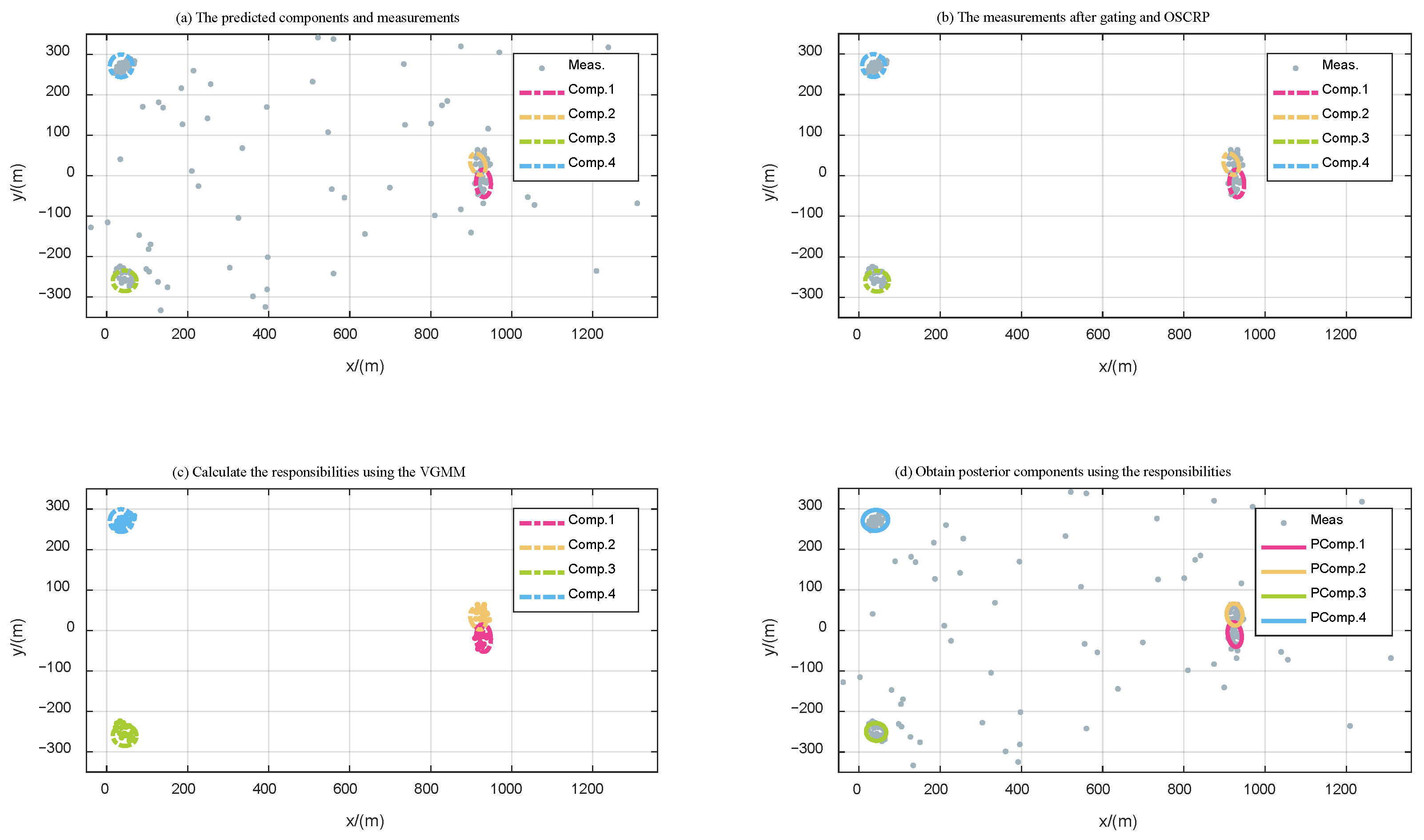
Due to the iterative nature of the VGMM, we use equivalent criteria for N ^ k 1 and N ^ k 2 to reduce the influence of clutter. However, their effectiveness is limited in dense clutter. At this point, thresholding and noise removal based on the marginal association probability with respect to the predicted PHD are needed. This procedure is called the One-Step Clutter Removal Process (OSCRP), and its details are described in [35]. For brevity, we do not repeat these procedures here. Instead, Figure 2 shows the processing flow in dense clutter that incorporates the OSCRP. Note that, in the third subfigure of Figure 2, we use component colors to indicate the label of each measurement.

5. Complexity Analysis

Figure 3 shows the flowchart of the proposed method from time k 1 to time k. The computational complexity of the proposed method is mainly concentrated in five parts.
  • P 1 : Time update
  • P 2 : ET-CPHD-based cardinality distribution estimation
  • P 3 : OSCRP
  • P 4 : VGMM for responsibility estimation
  • P 5 : SMU for each predicted component
Among these parts, P 3 , P 4 , and P 5 constitute the measurement update process. Compared with the standard ET-CPHD filter process flow [41], the main differences are the added steps P 3 and P 4 . When the number of measurements is M and the number of predicted components is N , the complexity of P3 can be expressed as O ( M N ) [35]. For  P 4 , the computational complexity of a single iteration of the VGMM is O M N according to Algorithm A1. Since the maximum number of iterations is limited to N emax , we have O ( P 2 ) = O N emax M N O ( M N ) . Both added steps P 3 and P 4 exhibit linear complexity with respect to the numbers of predicted components and measurements. Furthermore, the complexity of P1 is O N , and P2 has complexity O M 2 regardless of whether K-Means++ or DBSCAN is employed [46]. Finally, the complexity of P 5 is O P Y C P N · P · P , C , and we have
O N · P Y C P P < O P Y C P N · P · P , C < O N M · P Y C P P
P5 emerges as the key process affecting the overall complexity. Generally, P Y C P P < M and N M . Therefore, O P 5 O M 3 . The overall computational complexity of the ET-CPHD filter is O M 2 . Typically, N · P Y C P P exceeds M , leading to O ( P 5 ) > O M 2 . This indicates that, while the proposed filter has higher computational complexity than the ET-CPHD filter, it is no more than one order of magnitude higher, which is acceptable. In Figure 4, under ideal conditions—i.e., no target crossings or close-range motion, P D > 0.95 , P S > 0.98 , which permits the use of relatively sparse clustering parameters—we compare the proposed method with the conventional ET-CPHD method, namely the GIW-CPHD filter. We report the per-iteration computation time across different numbers of targets (from 2 to 10) and measurement densities ( ρ 1 : 10 4 measurements per unit volume, ρ 2 : 10 3 measurements per unit volume, ρ 3 : 10 2 measurements per unit volume). The results in Figure 4 further corroborate our analysis of the computational complexity.

6. Experimental Results

In this section, we evaluate the performance of the proposed method, the MEM-CPHD-VGMM filter, and compare it with the following methods:
  • MEM combined with the JIPDA algorithm for MTT [34], referred to as the MEM-JIPDA filter;
  • A widely used RMM-RFS-based method—here, we specifically select the CPHD-based implementation, referred to as the GIW-CPHD filter [17];
  • The ET-CPHD filter [41] integrated with the MEM, referred to as the MEM-CPHD filter;
  • A recent RFS-based PMB filter with the RMM, referred to as the GIW-PMB filter, implemented with reference to [47].
Note that the MEM-CPHD filter mentioned above has not been specifically proposed in the existing literature. Introducing this method helps to mitigate the impact of modeling differences on the final conclusion, thereby ensuring a fair comparison. Its implementation is straightforward and can be adapted from [31]. In the subsequent sections, we refer to each method by its abbreviation. For example, the MEM-JIPDA filter is simply denoted as MEM-JIPDA.
We present two comparative simulation experiments: the first is focused on unresolvable group targets, featuring multi-target merging and crossing events; the second is devoted to extended targets, simulating multiple vehicles traveling on a road. Using these two simulation experiments, we assess the applicability of our method to both types of target tracking. Experimental results and corresponding analyses are presented in Section 6.2 and Section 6.3, respectively. In addition, to further validate the practical applicability of our method, we present an experimental scenario based on a real dataset in Section 6.4. All units of the quantities in Section 6 are given in the international system.

6.1. Metrics

In evaluating the accuracy of the state estimation of targets with elliptical extents, ref. [48] has shown that the Gaussian Wasserstein distance (GWD) metric is an appropriate choice. The GWD between two elliptical targets [ s 1 , X 1 ] and [ s 2 , X 2 ] is calculated as
GWD 2 s 1 , X 1 , s 2 , X 2 s 1 s 2 2 2 + Tr X 1 + X 2 2 ( X 1 ) 1 2 X 2 ( X 1 ) 1 2
where s 1 and s 2 are the true ellipse center and the estimated ellipse center, respectively. ‘ · 2 ’ denotes the Euclidean norm. Similarly, X 1 and X 2 represent the extent matrices of the real ellipse and the estimated ellipse, respectively. As we use the orientation and the semi-axis lengths to describe the ellipse shape, i.e.,  x p = α , l 1 , l 2 T , the relationship between these parameters and the shape extent matrix X is
X = S S T
The calculation of S here can be found in Equation (7). To evaluate the tracking performance, the Generalized Optimal Sub-Pattern Assignment (GOSPA) [49] is used, integrating the GWD as a base metric; it can be split into localization errors (LOC), errors for missed targets (MIS), and errors for false targets (FAL). (We take the parameters for GOSPA as the location/extent error cutoff c = 40 and the order p = 1 .) In addition, based on the GOSPA results, we can further compute the average GOSPA and the mean target count error (MTCE) as quantitative metrics. The average GOSPA is
GOSPA avg = 1 N steps t = 1 N steps GOSPA t
where GOSPA t denotes the method’s GOSPA at time step t and N steps is the total number of time steps.
The MTCE is calculated as
MTCE = 1 N steps t = 1 N steps MIS t + FAL t = 1 N steps t = 1 N steps MIS t + 1 N steps t = 1 N steps FAL t = MIS avg + FAL avg
where MIS t and FAL t indicate the MIS and FAL of the method at time step k, respectively, and  MIS avg and FAL avg are the corresponding averages.
Moreover, to intuitively reflect changes in the number of targets, we also show the difference between the estimated number of targets and the true number via the estimated cardinality.

6.2. Experiment 1: Multi-Unresolvable Group Target Tracking

In this experiment, we consider a 2D scenario for MUGTT. Suppose that there are two launch airports that send out unmanned aerial vehicle (UAV) groups and use radar to capture the measurements of the UAV groups. A single UAV group can be regarded as an unresolvable group target and tracked as a whole. In the simulation, the sampling interval is set to T = 1 s, and the size of the simulation scenario is [−50, 1360] × [−350, 350]. The radar is located at the origin, the position of launch airport A is [0, −280], and the position of launch airport B is [0, 300].
At the initial time 1 s, Tar. 1 and Tar. 2 start from airport A and airport B on the left side of the scene, respectively, and move toward the right side of the scene. From 1 s to 40 s, these two targets gradually approach. After reaching a fairly close distance at 40 s, both targets move to the right together, with a constant speed, and remain parallel. In this parallel process, these two targets are so close to each other that their extents partially overlap.
After moving in parallel for a period of 47 s, at 87 s, these two targets gradually approach again and merge at 100 s. At this time, Tar. 2 can be regarded as dead in the scene, and the original Tar. 1 becomes the merged target with an expanded size and generates more measurements. Then, the merged target continues moving and leaves the scene at 120 s, at which time this merged target is deemed dead.
In addition, during the above process, at 81 s, airport A and airport B simultaneously send out Tar. 3 and Tar. 4, respectively. Their initial trajectories are the same as those of the first two targets. At 121 s, these two targets begin to maintain parallel movement at a close distance and then gradually approach each other at 168 s. Differing from the first two targets, these two targets are not merged but intersect between 176 s and 178 s. After this, these two targets maintain their respective movement directions and gradually move away until they leave the scene at 200 s. We show the trajectories of the four targets in Figure 5, using a color change from blue to yellow to indicate the evolution of time. The numbers of targets at different time steps and the corresponding situations are listed in Table 2. In addition, the simulation-related parameters are set as follows:
  • All targets are considered to have a unified state transition model that follows constant velocity dynamics. We assume that the shape of the target does not change during the time update, so we have
    Φ s = 1 T 0 1 I 2 ,   Φ p = I 3
    with the corresponding process noise matrix
    Q s = diag [ 5 , 10 ] I 2 ,   Q p = diag 0.02 , 1 , 1
  • For the measurements generated by the target, the non-homogeneous PPP with the Poisson parameter λ O = 20 is employed. The Poisson parameter of the merged target is 15. For clutter, we set the Poisson parameter λ C = 5 , so the scene’s measurement density is ρ = ( 4 λ O + λ C ) / ( 1410 × 700 ) = 8.61 × 10 4 . The measurement matrix H and the covariance of the additive measurement noise Q a are set as
    H = I 2 0 2 ,   Q a = 10 · I 2
  • The target’s detection probability and survival probability are taken as
    P D = 0.98 ,   P S = 1
  • There are two targets at the initial time. Their initial positions are set to be the same as the positions of the two launch points; namely, we set x ^ 0 s 1 = [ 0 , 300 , 0 , 0 ] T and x ^ 0 s 2 = [ 0 , 300 , 0 , 0 ] T , as well as the corresponding initial shape states x ^ 0 p 1 = x ^ 0 p 2 = [ 0 , 30 , 30 ] T . The birth components of each filter at each time are consistent with the initial states of these two targets. The probability mass function of the birth components in Equation (16) is set to
    M β , k n = 0.90 ,     n = 0 0.075 ,   n = 1 0.025 ,   n = 2 , 3 0 ,       otherwise
  • It should be noted that, for the GIW-CPHD filter, although the shape states of each component cannot be explicitly specified, its extent matrix can be calculated via Equation (65). For the inverse Wishart distribution of the birth components, we set its parameters to
    v = 2 · d + 3 = 7
    V = 900 · I 2
    to ensure that the extent of its birth components is consistent with other filters.
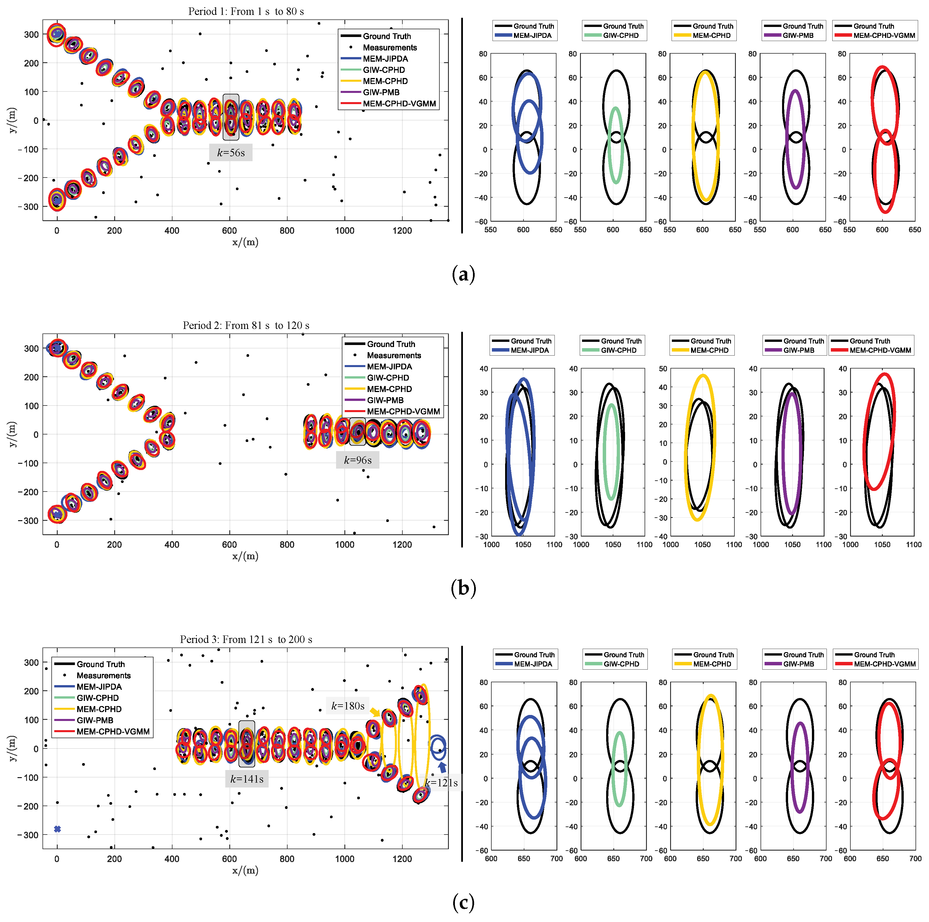
We perform 100 MC runs for each filter (MATLAB R2023b codes are run on workstations with 2.8 GHz Intel Core i9-10900 processors) and calculate the averages of the metrics mentioned in Section 6.1 as the final result. An example MC run of Experiment 1 is provided in Figure 6. For clarity, we divide it into three segments, i.e., Period 1, from 1 s to 80 s; Period 2, from 81 s to 120 s; and Period 3, from 121 s to 200 s. For each period, we select a representative time slice to present the estimation of each filter on the right side of the figure, including 56 s in Period 1, 106 s in Period 2, and 141 s in Period 3.
It can be seen from Figure 6 that all filters can capture the birth situations of the targets. However, the performance of each filter is different. When two targets maintain close proximity and parallel motion, GIW-CPHD, MEM-CPHD, and GIW-PMB all exhibit erroneous “state fusion”, as seen in the 56 s slice of Period 1 and the 141 s slice of Period 3.
In terms of estimating the extent of the target, GIW-CPHD and GIW-PMB perform more poorly than MEM-CPHD. They have small estimations of the targets’ extent and cannot accurately capture the expansion of the merged target’s shape, as seen in the 106 s slice of Period 2. In addition, another shortcoming of MEM-CPHD is that it cannot track intersecting targets. For the two intersecting targets, it erroneously considers them as one target, and, in the subsequent process, the erroneous shape estimation continues to propagate, as seen in the 180 s slice of Period 3, marked by the yellow arrow in Figure 6c. MEM-JIPDA can effectively distinguish between two parallel targets at close range, but, when the targets disappear or merge, MEM-JIPDA performs poorly. This is intuitively reflected in the 106 s slice of Period 2; MEM-JIPDA overestimates the number of targets and provides an additional state estimate, which is due to its insensitivity to target merging. The same error also occurs when the merged target disappears; MEM-JIPDA considers that it still exists and produces redundant state estimates, as seen in the 121 s slice of Period 3, marked by the blue arrow in Figure 6c.
Our proposed MEM-CPHD-VGMM has better performance than the other filters. For two targets moving in parallel at close range, it can effectively distinguish and provide shape estimation results for these targets without “state fusion”, as seen in the 56 s slice of Period 1 and the 141 s slice of Period 3. For the merged target, it can also accurately estimate the expanded extent, as seen in the 106 s slice of Period 2. Moreover, it can handle situations where targets disappear or intersect, without errors such as missed or false estimates.
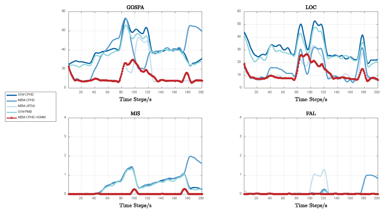
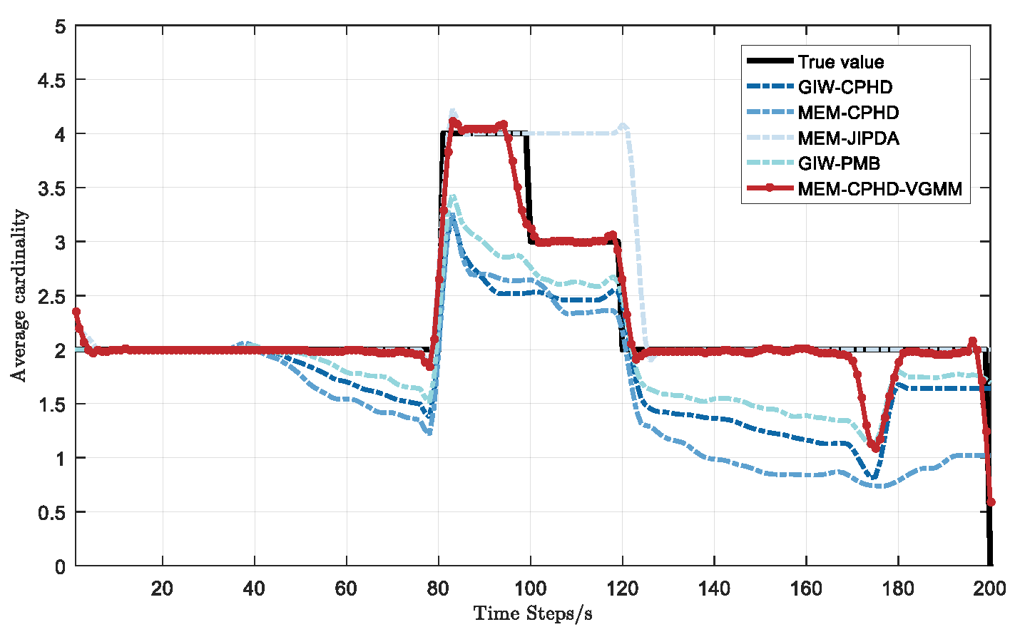
We further demonstrate the GOSPA of each filter in Figure 7, and the estimated cardinality against time for the filters is shown in Figure 8. In the left half of Table 3, we also report the MTCE of each filter.
The GOSPA results in Figure 7 comprehensively reflect the performance of each filter, which can be summarized as follows.
  • Regarding GIW-CPHD, it has the worst performance in shape estimation; therefore, compared to other filters, it has a significantly larger LOC. GIW-PMB shows the second-worst shape estimation; although its LOC decreases, the reduction is marginal.
  • For MEM-CPHD, its accuracy in shape estimation is improved compared to GIW-CPHD and GIW-PMB, but both have the disadvantage of state fusion for nearby targets. Therefore, their MIS increases from 40 s to 100 s and from 120 s to 168 s, resulting in a larger GOSPA during these time periods. Differently, MEM-CPHD still has erroneous estimation fusion after target crossover. Therefore, after 178 s, the MIS values of GIW-CPHD and GIW-PMB return to normal, but the MIS of MEM-CPHD still shows an upward trend, accompanied by an increase in its FAL. This results in MEM-CPHD having the maximum GOSPA after 178 s.
  • For MEM-JIPDA, it has a stable MIS. However, due to its insensitivity to target merging and disappearance, there will be redundant state estimates after the merging of two targets, which leads to a peak in its FAL after 100 s, causing an increase in its GOSPA.
  • Regarding our proposed MEM-CPHD-VGMM, its LOC, MIS, and FAL all indicate the best performance, meaning that it has the lowest GOSPA among all filters. However, when two targets remain in close proximity for a prolonged period, MEM-CPHD-VGMM still tends to treat the two targets as one, resulting in a small peak in its MIS at around 95–105 s and 170–180 s, which leads to a slight increase in its GOSPA during these time periods.
From the cardinality distribution estimation results shown in Figure 8 and the left-side MTCE results in Table 3, we can see that GIW-CPHD, MEM-CPHD, and GIW-PMB persistently underestimate cardinality due to incorrect state fusion. Moreover, MEM-CPHD still has unreasonable state fusion after target crossing, resulting in the largest deviation in cardinality estimation after 180 s. MEM-JIPDA provides redundant state estimation for the merged target, resulting in a larger cardinality estimate after 100 s. In contrast, our proposed MEM-CPHD-VGMM only shows a deviation in cardinality estimation at around 95–105 s and 170–180 s, and it maintains the minimum deviation in other time periods, reflecting the accuracy of the proposed method.

6.3. Experiment 2: Multi-Extended Target Tracking

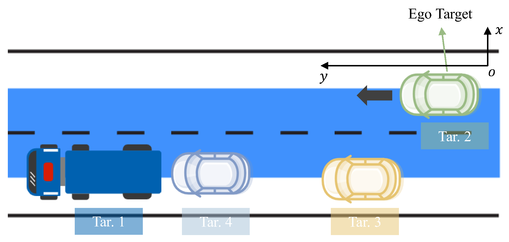
In this experiment, we further demonstrate the advantages of our method in tracking multiple extended targets. The construction of the simulation scenario is based on the ‘Automated Driving Toolbox’ (see https://ww2.mathworks.cn/help/releases/R2023b/driving/index.html (accessed on 18 Jun 2024) for details) officially provided by MATLAB, which provides algorithms and tools for designing and simulating autonomous driving systems. Using this toolbox, we simulate multiple vehicles traveling on an urban road; each vehicle is treated as an extended target. Additionally, we simulate a front-mounted mmWave radar for the ego vehicle to collect measurements and transform them from the ego frame coordinates to global Cartesian coordinates.
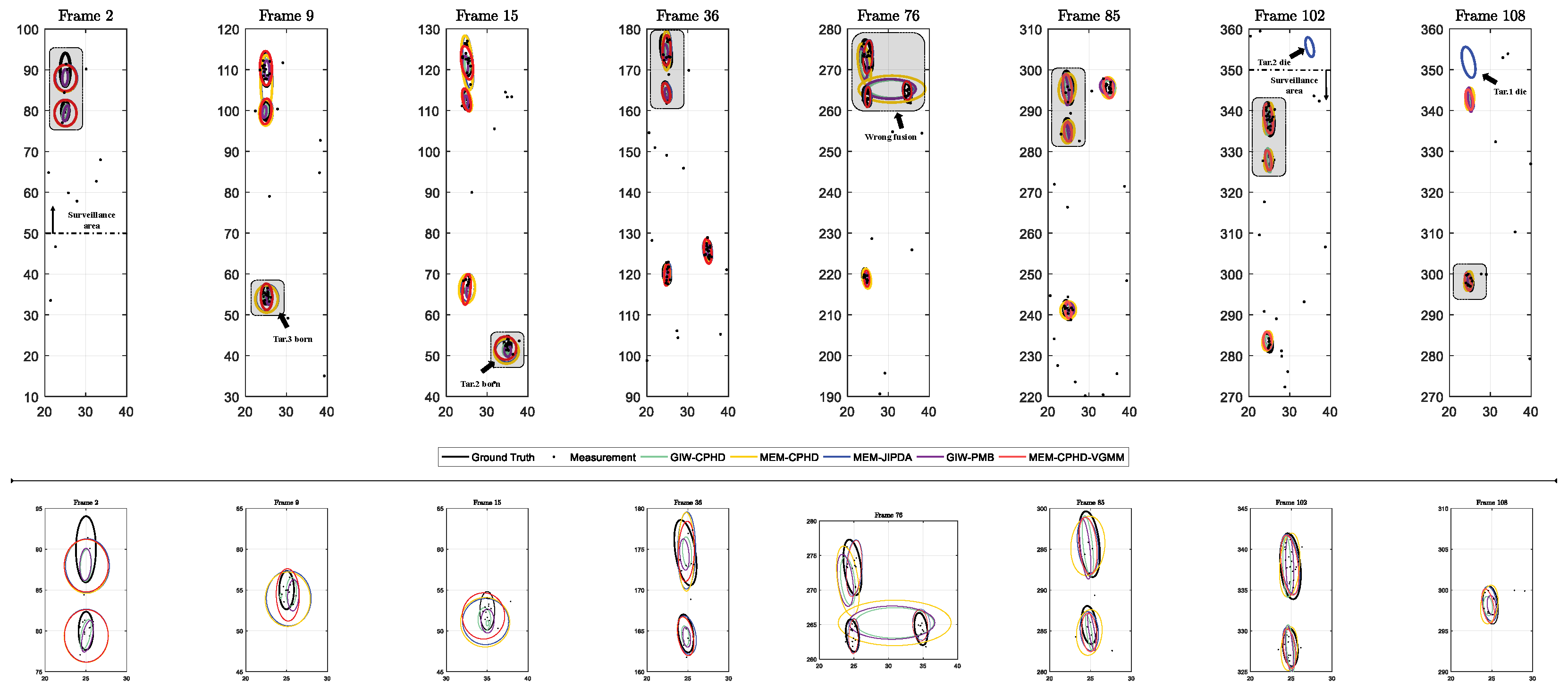
Figure 9 shows a schematic diagram of this simulation; there are four vehicles involved in the scene, including one truck and three saloon cars. The simulation scenario can be described as follows. The size of the surveillance area is [50, 350] × [20, 40]. The entire simulation process contains 114 frames, and the time interval of each frame is T = 1 s. At the initial frame, there are only Tar. 1 and Tar. 4 in the scene, and they are located in the bottom lane, on the right side of the road, and drive forward at a constant speed. Then, at the 9th frame, Tar. 3 enters the surveillance area and drives behind the first two targets. At the 15th frame, Tar. 2 enters the surveillance area from the top lane. Thus, the number of targets increases to 4. After this, this number remains at 4 for 87 frames, during which Tar. 2 overtakes the other three targets. At the 101st frame, Tar. 2 leaves the surveillance area. Subsequently, Tar. 1 and Tar. 4 leave the surveillance area at the 107th frame and 111th frame, respectively. Finally, at the 114th frame, the entire process ends with Tar. 3 still inside the surveillance area. The specific information for each target, as well as the frames of its birth and death, is listed in Table 4.
The settings of the state transition matrix, the observation matrix, the detection probability, and the survival probability of the target are consistent with Experiment 1. Due to the reduced size of the scene, we adjust the process noise, the observation noise, and the relevant Poisson parameters as
Q s = diag [ 5 , 1 ] I 2 ,   Q p = diag 0.02 , 1 , 1 ,   Q a = 1.5 · I 2
λ O = 8 ,   λ C = 5 , ρ = 6.17 × 10 3
The birth components of each filter at each frame are set as x ^ 0 s 1 = 250 , 500 , 0 , 0 T , x ^ 0 p 1 = 0 , 30 , 30 T and x ^ 0 s 2 = 350 , 500 , 0 , 0 T , x ^ 0 p 2 = [ 0 , 30 , 30 ] T . We choose the same M β , k · as in Experiment 1. Then, the parameters of GOSPA are adjusted to the location error cut-off c = 20 and the order p = 1.
We select 8 important frames, which are the frames 2 ,   9 ,   15 ,   36 ,   76 ,   85 ,   102 ,   108 . The slicing of these frames in an example MC run with the estimation results is shown in Figure 10, and we include some arrow marks in these slices for illustration. In addition, we highlight the important area in each frame and further display details below the corresponding frame. Note that, at the 76th frame, GIW-CPHD, MEM-CPHD, and GIW-PMB all show incorrect state fusion, which occurs when Tar. 2 catches up with Tar. 4 and the intertarget distance becomes small. In the following 85th frame, the state fusion disappears as Tar. 2 surpasses Tar. 3.
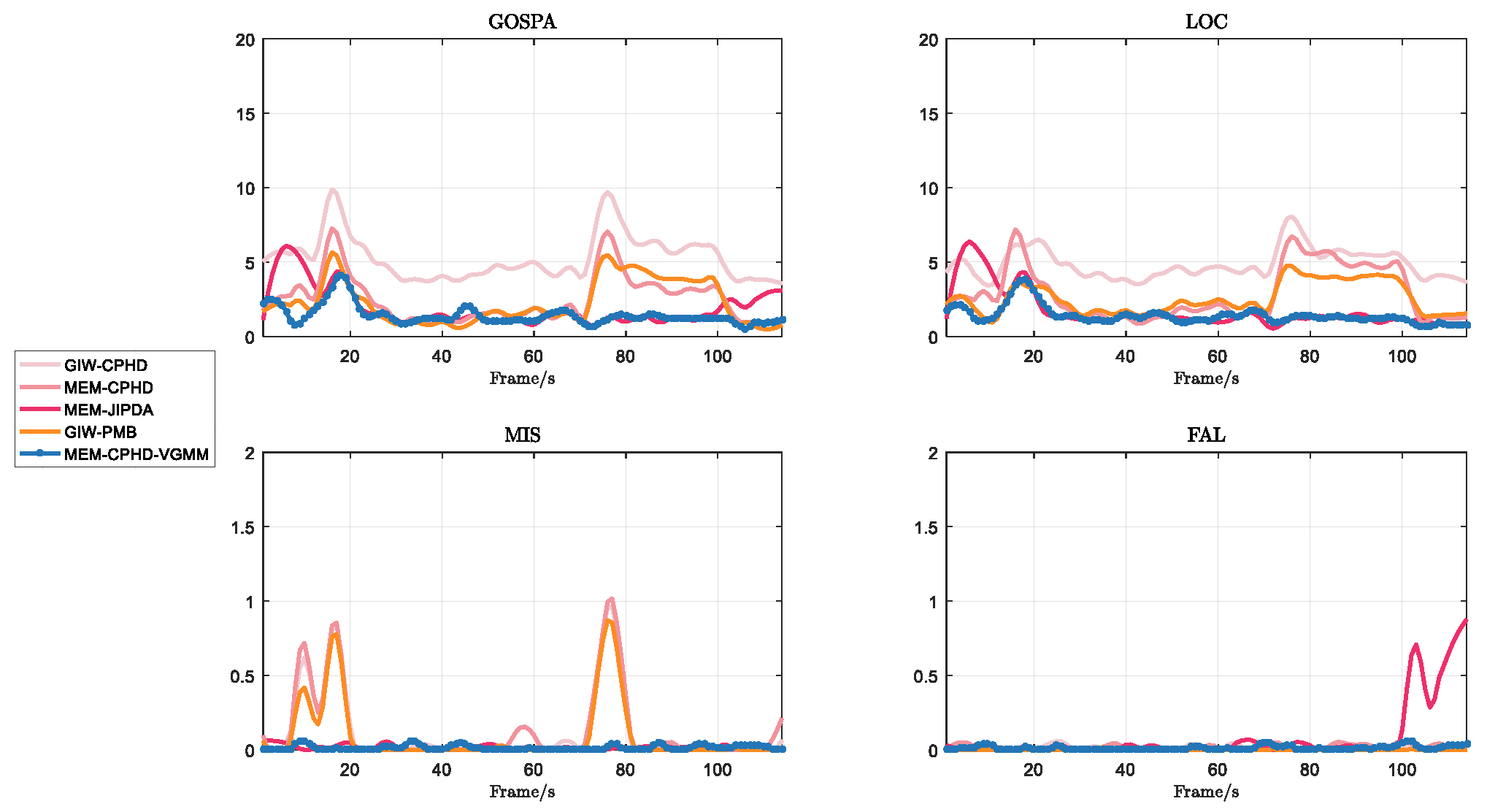
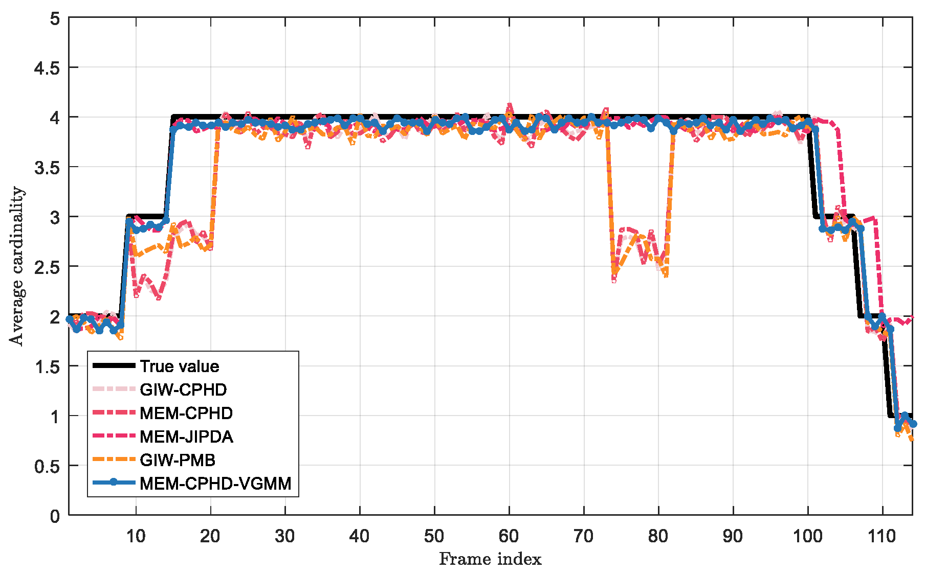
The GOSPA and the estimated cardinality obtained through 100 MC runs are shown in Figure 11 and Figure 12, respectively, while the right half of Table 3 lists the MTCE for each filter. The results in Figure 11 and Figure 12, and the right side of Table 3 demonstrate the conclusion reached in Experiment 1; namely, MEM-JIPDA is insensitive to the death of targets and this leads to the overestimation of the number of targets. Therefore, after the 100th frame, its FAL rises and diverges. Moreover, GIW-CPHD, MEM-CPHD, and GIW-PMB all suffer from state fusion defects in close-proximity target tracking, resulting in elevated MIS and LOC values between frames 17 and 20 and frames 75 and 80. During these periods, Tar. 2 is in close proximity to Tar. 3 and Tar. 4, respectively. By comparison, our proposed MEM-CPHD-VGMM demonstrates superior overall performance, exhibiting the lowest GOSPA and the most precise cardinality estimation.
We present in Table 5 the average runtime per MC run and the time consumed per iteration cycle for each filter. It can be observed that MEM-CPHD-VGMM is close to but higher than MEM-JIPDA, with computational complexity of O M 2 [34]. Additionally, the integration of the VGMM for responsibility computation results in increased computational complexity relative to GIW-CPHD, MEM-CPHD, and GIW-PMB, although the overhead remains computationally tractable. These results are consistent with the conclusions of the algorithm complexity analysis conducted in Section 5.
Finally, for both experimental scenarios, we implement various modifications based on the original parameter settings, and we show the average GOSPA for different simulation parameters in Table 6.
These modifications include lower target detection probabilities, reduced target survival probabilities, increased measurement noise, and denser clutter distributions. As expected, when the detection probability and survival probability decrease, or when clutter density and measurement covariance increase, all filters exhibit degraded performance. Nevertheless, our proposed MEM-CPHD-VGMM consistently maintains the lowest GOSPA across all conditions, as emphasized by the bold formatting in Table 6, indicating its robust stability and superior adaptability to diverse environments.

6.4. Experiment 3: Experiment with Real Data in the SIND Dataset

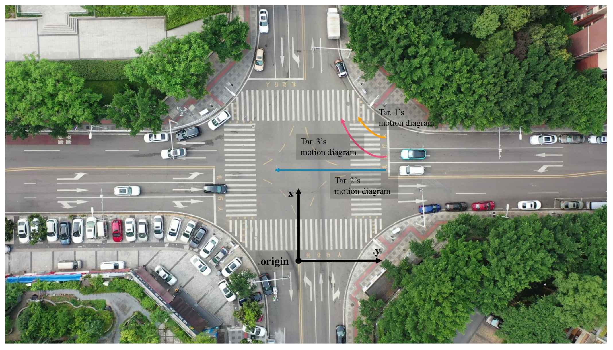
In this section, we verify the performance of the proposed method with real data from the SIND dataset. We select SIND as the dataset for our experiment. It is suitable for intelligent transportation systems and includes surveillance information from signalized intersections across multiple Chinese cities. We choose one signalized intersection in Chongqing, as shown in Figure 13; the selected site includes 7 h of recording and over 13,000 traffic participants. We extract a 90 s segment that includes target births and deaths, as well as the motion of multiple targets in close proximity. SIND provides target bounding boxes, so ground truth is readily available. Following the processing described in ([25], Section 6B), LiDAR measurements of targets are generated and further transformed into the global Cartesian frame. Measurements are taken at 1 s per frame. Therefore, Experiment 3 contains 90 frames. More details of SIND are provided in [50].
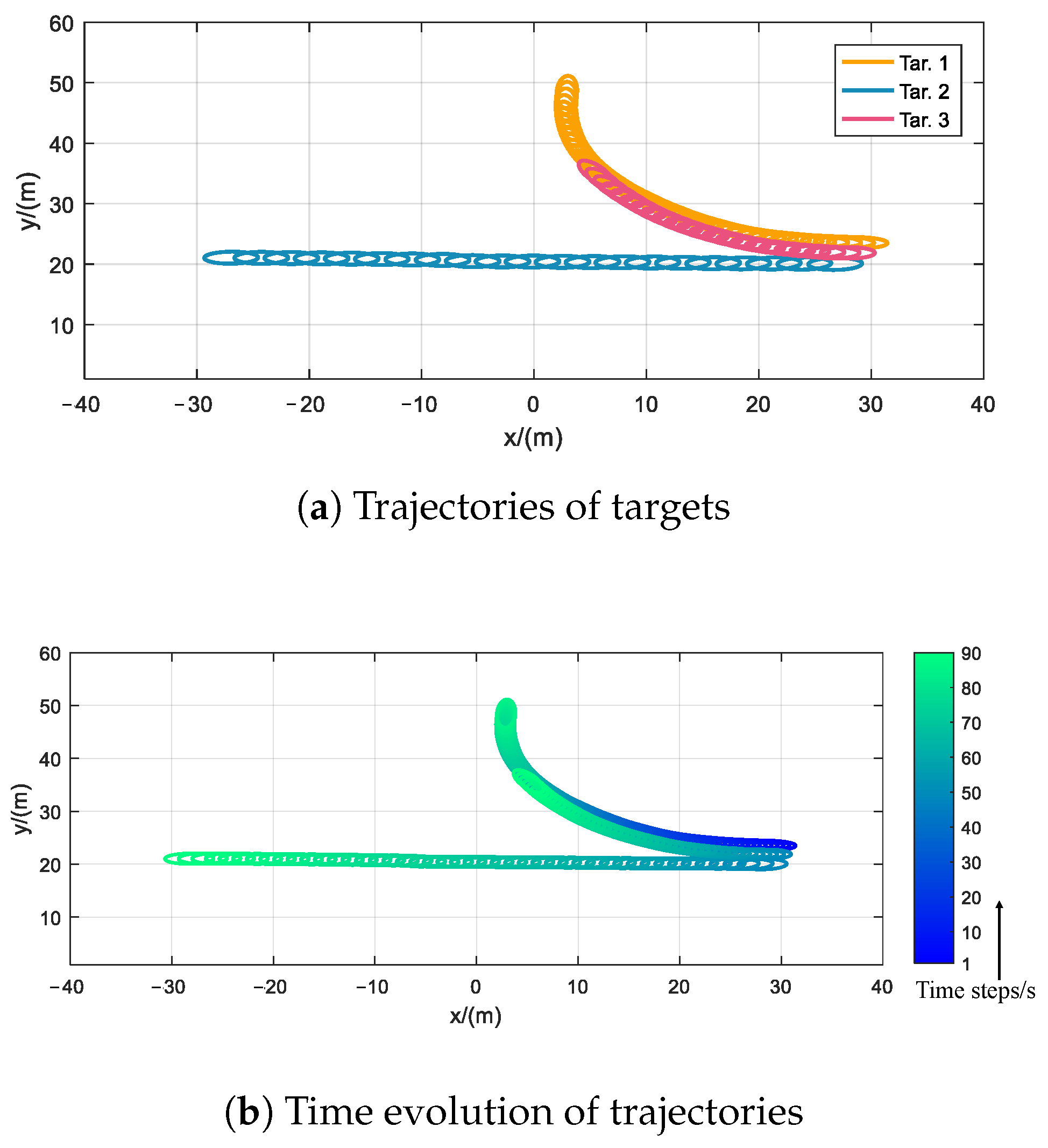
As shown in Figure 14, the scene in Experiment 3 spans [−40, 40] × [0, 60] and contains three targets; their trajectories are shown in Figure 14a. The overall motion is as follows. In frame 1, Tar. 1 appears, turns right at the intersection, and then goes straight. At frame 48, Tar. 2 and Tar. 3 are appear simultaneously; they move in the same direction and are closely spaced. Then, at the intersection, Tar. 3 turns right and then goes straight, while Tar. 2 continues straight, so the two targets gradually diverge. At frame 85, Tar. 1 leaves the scene and is considered dead, while Tar. 2 and Tar. 3 continue moving until frame 90. The scene ends. The evolution of the targets’ trajectories over time is depicted in Figure 14b.
We compare our method with four other filters in this scenario. The evaluation metrics remain the GOSPA, estimated cardinality, and runtime. Because the scale of this scenario is similar to that of Experiment 2, the parameter settings for all filters and metric computations are kept consistent with those in Experiment 2.
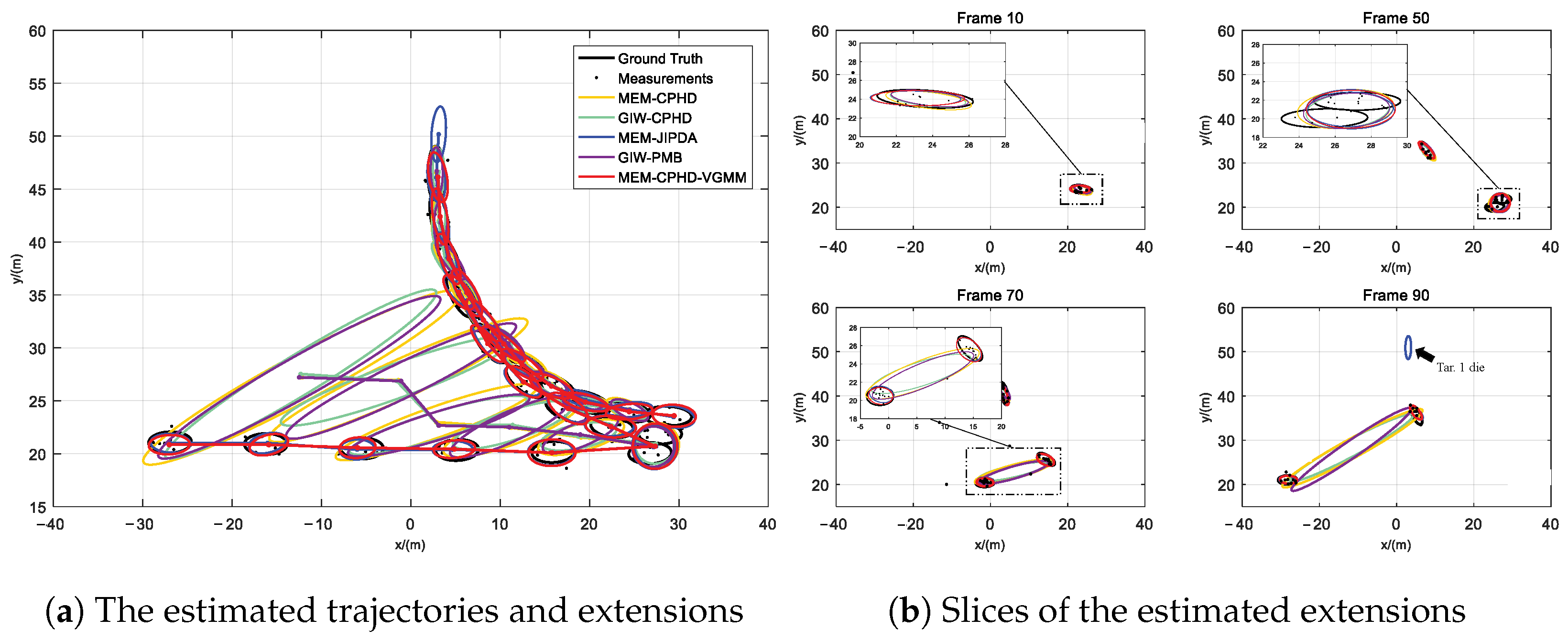
In Figure 15, we present the estimated trajectories and extensions for each method. We also select four representative frames—10, 50, 70, and 90—to illustrate the details of each method’s extent estimates. As can be seen, GIW-CPHD, GIW-PMB, and MEM-CPHD suffer from severe state fusion. At frame 48, all three methods treat Tar. 2 and Tar. 3, which appear simultaneously and move in close proximity, as a single target. Our method avoids this error and unambiguously estimates the states of Tar. 2 and Tar. 3 separately. MEM-JIPDA appears to perform similarly to our method, but it remains insensitive to disappearing targets. As indicated by the arrow in Figure 15b, at frame 90, Tar. 1 has already left the scene, yet MEM-JIPDA continues to estimate its state, which is clearly redundant.
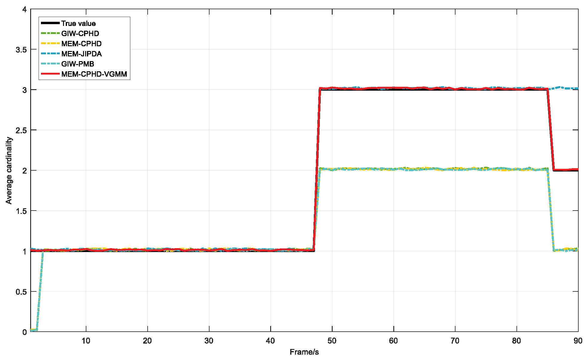
Figure 16 and Figure 17 show, respectively, the GOSPA and estimated cardinality for Experiment 3, and the MTCE of the filters is recorded in Table 7. These results provide stronger evidence for our observations. Because GIW-CPHD, GIW-PMB, and MEM-CPHD exhibit erroneous state fusion, their GOSPA increases progressively after frame 48, and their estimated cardinalities fall below the ground truth. In contrast, MEM-JIPDA and our method avoid state fusion and thus achieve lower GOSPA after frame 48. However, due to MEM-JIPDA’s redundant estimates for dead targets, its GOSPA rises after frame 95. Overall, our method attains the lowest GOSPA and the most accurate cardinality estimates.
Finally, Table 8 reports the per-iteration runtime of each method. In the scene generated from real data, owing to reduced scene clutter, our method is more time-consuming than the others, but it completes each iteration in less than the 1 s time interval, satisfying the real-time requirements.

7. Discussion

The method proposed in this paper builds on the CPHD filtering framework and combines the VGMM with the MEM to achieve the precise tracking of multiple, closely spaced targets. Because the number of PHD components can grow exponentially, pruning and merging are necessary. We can implement this series of procedures following [16], but our handling of component merging is slightly different. For component merging, since the target state is represented by two decoupled Gaussian distributions, we can specify separate merging thresholds for kinematics and shape. In addition, drawing on the existing literature, we discuss the scalability of our proposed method and outline future research directions along three dimensions: parametric modeling, shape–model integration, and trajectory generation.
In terms of parametric modeling, note that, in this work, we treat the target’s measurement rate and detection probability as constants, while, in practice, these parameters are typically time-varying. Following [47,51], they can be modeled as unknowns with gamma and beta priors and estimated within the filtering recursion. Due to the conjugacy of these distributions, they can be integrated into our method with minimal modification.
Then, regarding the target shape model, we model the target extent as an ellipse, which offers parametric simplicity and broad applicability. However, some applications require more precise shape discrimination. In such cases, an elliptical approximation is insufficient, and more expressive representations are needed, such as star convex shapes, multidimensional splines, triangular shapes, and other complex geometries. Under these models, the spatial distribution of measurements is often non-Gaussian, which prevents Gaussian process models [52], random hypersurface models [53], random triangle models [54], and B-spline models [55] from being embedded directly into our framework. A practical approach is to approximate their measurement distributions as Gaussians by minimizing the KLD, and integrating these models on this basis represents a direction for future work.
Finally, as for trajectory generation, since our method functions as a filter, it is currently unable to produce stable target tracks. The recently introduced trajectory set theory [20,56,57] enables track generation and maintenance for RFS-based filters, and combining our method with trajectory set theory could yield a tracker in the strict sense.

8. Conclusions

In this work, we present an MTT method for the tracking of multiple extended targets or unresolvable group targets. The proposed method is based on the CPHD filtering framework and involves estimating the states of the targets using the MEM. During the measurement update, we employ the VGMM to compute the responsibilities of predicted components for each measurement. We then use these responsibilities to update the component states. In addition, we demonstrate the performance of the proposed method through simulations on both unresolvable group targets and extended targets. The experiments show that the proposed method significantly improves the estimation accuracy compared to existing methods in challenging MTT scenes, especially for closely spaced targets.

Author Contributions

Conceptualization, Y.C. (Yuanhao Cheng) and Y.C. (Yunhe Cao); methodology, Y.C. (Yuanhao Cheng); software, Y.C. (Yuanhao Cheng); validation, Y.C. (Yuanhao Cheng); formal analysis, J.F.; investigation, Y.Z.; resources, Y.Z.; data curation, Y.C. (Yuanhao Cheng) and J.F.; writing—original draft preparation, Y.C. (Yuanhao Cheng); writing—review and editing, Y.C. (Yuanhao Cheng) and T.-S.Y.; visualization, Y.C. (Yuanhao Cheng); supervision, Y.C. (Yunhe Cao) and T.-S.Y.; project administration, Y.C. (Yuanhao Cheng); funding acquisition, Y.C. (Yunhe Cao). All authors have read and agreed to the published version of the manuscript.

Funding

This research was funded by the National Natural Science Foundation of China under grant number 61771367.

Data Availability Statement

The data presented in this study include SIND, which is openly available in [SIND: A drone dataset at signalized intersection in China] at [10.1109/ITSC55140.2022.9921959], reference number [50]. Github: https://github.com/SOTIF-AVLab/SinD, accessed on 25 October 2025.

Conflicts of Interest

The authors declare no conflicts of interest.

Abbreviations

METTMultiple Extended Target Tracking
MUGTTMultiple Unresolvable Group Target Tracking
RMMRandom Matrix Model
CPHDCardinality Probabilistic Hypothesis Density
SMUSequential Measurement Update
OSCRPOne-Step Clutter Removal Process
MTCEMean Target Count Error

Appendix A. Notations and Corresponding Explanations

Table A1. Notations.
  • Real number field R ; positive integer field Z + ; set of real horizontal vectors of length n is represented with R n ; set of real matrices of size m × n is represented with R m × n .
  • Set of symmetric positive definite and semi-definite matrices of size n × n is represented with S + + n and S + n , respectively.
  • N x ;   μ , Σ represents the multivariate Gaussian distribution with mean vector μ R n x and covariance matrix Σ S + + n x .
  • W X ;   υ , V denotes the Wishart distribution with degrees of freedom υ R and semi-definite scale matrix V S + n X , satisfying
    W X ;   υ , V X υ 2 e tr 1 2 X 1 V
  • D Π ;   A denotes the Dirichlet distribution with parameter set A = α i i = 1 L , satisfying
    D Π ;   A l = 1 L Π l α l 1
  • δ a b is the delta function that satisfies δ a b = 1 if a b or  δ a b = 0 otherwise.
  • tr A denotes the trace of the matrix A; a ¯ represents the expectation of variable a, i.e.,  E a ; a T means finding the transpose of a; a ! means calculating the factorial of a; A denotes the determinant of the matrix A. If variable A is treated as a set A , then A represents the cardinality of set A .
  • The quadratic forms x T Ax and outer products x x T are written as x T A · and x · T , respectively, to avoid duplicating long expressions.
  • Some important variables and their meanings:
-
ξ and Ξ : target’s augmented state and corresponding covariance
-
x s and C s : target’s kinematic state and corresponding covariance
-
x p and C p : target’s shape state and corresponding covariance
-
X : state parameter set
-
y : measurement; Y : pseudo-measurement
-
Y : measurement set
-
i: measurement index; j: PHD component index
-
Q or Q : covariance of Gaussian white noise
-
Φ k s or Φ s : kinematic state transition matrix
-
Φ p s or Φ p : shape state transition matrix
-
H or H : measurement matrix
-
S: shape description matrix
-
π and Π : mixing coefficient and corresponding set
-
z and Z : latent variable and corresponding set
-
μ and Σ : mean and covariance of Gaussian distribution
-
Ψ : parameter set of Gaussian distribution
-
U : set of Gaussian mean
-
E : set of Gaussian covariance
-
q · : variational density
-
D · : probability hypothesis density (PHD)
-
M · : cardinality distribution
-
w: weight of each component in PHD
-
J: number of components in PHD
-
ϱ : responsibility
-
P : measurement partition
-
C : measurement cell
-
O D · or P D : detection probability
-
O S · or P S : survival probability
-
λ O : Poisson measurement rate of target
-
λ C : Poisson clutter rate
-
ρ : measurement density

Appendix B. Proof of Theorem 1

Proof of Theorem 1 Before proving Theorem 1, we introduce the PDA measurement update for the point target (PTar). Let x denote the state parameter of the PTar and  X represent the corresponding covariance. If the number of PTars is fixed at n , then the predicted state of the PTars at time k can be expressed as a set X ˙ ^ k | k 1 = x ^ k | k 1 ( j ) , X ^ k | k 1 ( j ) j = 1 n . Given the measurement set Y k = y k i i = 1 m k at time k, the PDA measurement update for the j-th PTar can be written as [45]
x ^ k | k ( j ) = x ^ k | k 1 ( j ) + κ k ( j ) y ˜ k ( j )
y ˜ k ( j ) = i = 1 m k p i ( j ) y ¯ k i ( j )
y ¯ k i ( j ) = y k i H · x ^ k | k 1 ( j )
κ k ( j ) = X ^ k | k 1 ( j ) H T Υ k | k 1 ( j ) 1
Υ k | k 1 ( j ) = H X ^ k | k 1 ( j ) H T + R
X ^ k | k ( j ) = X ^ k | k 0 ( j ) + d X ^ k ( j )
X ^ k | k 0 j = p 0 ( j )   X ^ k | k 1 ( j ) + 1 p 0 ( j ) X ^ k | k ( j )
d X ^ k ( j ) = κ k ( j ) i = 1 m k p i ( j ) y ¯ k i ( j ) y ¯ k i ( j ) T y ˜ k ( j ) y ˜ k ( j ) T κ k ( j ) T = p 1 ( j ) 1 p 1 ( j ) κ k ( j ) y ¯ k i ( j ) y ¯ k i ( j ) T κ k ( j ) T
X ^ k | k ( j ) = I κ k ( j ) H X ^ k | k 1 ( j )
where p i ( j ) is the association probability that measurement y k i is assigned to the j-th PTar in a single hypothesis. For the j-th PTar, we assume that it produces at most one measurement at time k and that there are m k + 1 hypotheses for each PTar. p 0 ( j ) is the probability that there is no measurement from the correlation gate of the j-th PTar, κ k ( j ) is the Kalman gain, and R represents measurement noise.
We now discuss using the i-th measurement y k i to update the kinematic state x s ( j ) of the j-th target, as described in Section 2, at time k. In fact, since the kinematic state describes the dynamics of the center of the target, the center can be regarded as a PTar, and the measurement y k i can be used to perform the PDA measurement update on this PTar. Based on C 1 and C 2 in Section 4.2, the prior state is the result of updating the ( i 1 ) -th measurement, so Equation (A1) becomes
x ^ k | k s ( j ) [ i ] = x ^ k | k s ( j ) [ i 1 ] + κ k ( j ) y ˜ k ( j )
Meanwhile, the probability p i ( j ) in Equation (A2) reduces to the marginal association probability ϵ i , j that measurement y k i belongs to the j-th target, and we have
ϵ i , j = p θ i = j | Y k , X k = θ   with   θ i = j p θ | Y k , X k = i = 1 m k p i ( j )
where the set X k contains the target states, and the symbol ‘ θ ’ denotes the association hypothesis, which is a random vector of size ‘ 1 × m k ’ and satisfies
θ i = 0 ,   if   y k i   is   a   clutter j ,   if   y k i   is   assigned   to   the   i - th   target ,   j 1 , , n
Since the responsibility in Equation (27) represents the association probability between the measurement y k i and the j-th component, and this probability is independent across components, each component corresponds to the potential target. Thus, ϱ ^ k i ( j ) has the same meaning as the marginal association probability ϵ i , j , i.e.,
ϵ i , j ϱ ^ k i ( j )
At this point, the measurements used for the update are the measurement cell P , C = y k P , C , i i = 1 P , C . Therefore, Equation (A2) is equivalent to
y ˜ k ( j ) = i = 1 m k p i ( j ) y ¯ k i ( j ) = ϱ ^ k i ( j ) y k P , C , i H x k | k s ( j ) [ i 1 ]
Together with Equationa (A4) and (A10), we have
x ^ k | k s ( j ) [ i ] = x ^ k | k s ( j ) [ i 1 ] + κ k ( j ) ϱ ^ k i ( j ) y k P , C , i H x k | k s ( j ) [ i 1 ] = x ^ k | k s ( j ) [ i 1 ] + K k ( j ) y k P , C , i H x k | k s ( j ) [ i 1 ]
K k ( j ) = ϱ ^ k i ( j ) X ^ k | k 1 ( j ) H T Υ k | k 1 ( j ) 1 = ϱ ^ k i ( j ) C k | k s ( j ) [ i 1 ] H T C k | k y ( j ) [ i ] 1 = ϱ ^ k i ( j ) C k | k s y   ( j ) [ i ] C k | k y [ i ] 1
The last step of Equation (A16) holds because C k | k s ( j ) [ i 1 ] H T = C k | k s y ( j ) [ i ] as in Equation (53). Note that, in Equation (A16), we replace X ^ k | k 1 ( j ) and Υ k | k 1 ( j ) with C k | k s ( j ) [ i 1 ] and C k | k y ( j ) [ i ] , respectively. This is reasonable since they have the same meaning; only the context changes from a point target to an extended target or an unresolvable group target.
Since y ¯ k i ( j ) = H · x k | k s ( j ) [ i 1 ] , Equation (A15) can be further written as
x ^ k | k s ( j ) [ i ] = x ^ k | k s ( j ) [ i 1 ] + ϱ ^ k i ( j ) C k | k s y ( j ) [ i ] C k | k y ( j ) [ i ] 1 y k P , C , i y ¯ k i ( j )
Note that
p 0 ( j ) = 1 ϵ i , j = 1 ϱ ^ k i ( j )
p 1 ( j ) = ϱ ^ k i ( j )
Thus, Equation (A7) can be rewritten as Equation (A20), and we use the equation H C k | k s ( j ) [ i 1 ] =   C k | k s ( j ) [ i 1 ] H T T = C k | k s y   ( j ) [ i ] T in the last step.
C k | k s 0 ( j ) [ i ] = 1 ϱ ^ k i ( j ) C k | k s j [ i 1 ] + ϱ ^ k i ( j ) C k | k s j [ i 1 ] ϱ ^ k i ( j ) C k | k s y   ( j ) [ i ] C k | k y ( j ) [ i ] 1 H C k | k s ( j ) [ i 1 ] = 1 ϱ ^ k i ( j ) C k | k s ( j ) [ i 1 ] + ϱ ^ k i ( j ) C k | k s ( j ) [ i 1 ] ϱ ^ k i ( j ) C k | k s y   ( j ) [ i ] C k | k y ( j ) [ i ] 1 C k | k s y   ( j ) [ i ]   T
d C k s ( j ) [ i ] = ϱ ^ k i ( j ) 1 ϱ ^ k i ( j ) ϱ ^ k i ( j ) C k | k s y   ( j ) [ i ] C k | k y ( j ) [ i ] 1 y k P , C , i y ¯ k i ( j ) × ϱ ^ k i ( j ) C k | k s y   ( j ) [ i ] C k | k y ( j ) [ i ] 1 y k P , C , i y ¯ k i ( j ) T
Meanwhile, Equation (A8) can be rewritten as Equation (A21). We have
d C k s ( j ) [ i ] = ϱ ^ k i ( j ) 1 ϱ ^ k i ( j ) ϱ ^ k i ( j ) ϱ ^ k i j T
C k | k s y j [ i ] C k | k y ( j ) [ i ] 1 y k P , C , i y ¯ k i ( j )
Substituting Equations (A20) and (A22) into Equation (A6), we obtain
C k | k s ( j ) [ i ] = C k | k s 0 ( j ) [ i ] + d C k s ( j ) [ i ] = 1 ϱ ^ k j i C k | k s i [ j 1 ] + ϱ ^ k j i C k | k s i [ j 1 ] ϱ ^ k i j C k | k s y   ( j ) [ i ] C k | k y ( j ) [ i ] 1 C k | k s y   ( j ) [ i ] T + ϱ ^ k i ( j ) 1 ϱ ^ k i ( j ) ϱ ^ k i ( j ) ϱ ^ k i ( j ) T = C k | k s ( j ) [ i 1 ] ϱ ^ k i ( j ) C k | k s y ( j ) [ i ] C k | k y ( j ) [ i ] 1 C k | k s y   ( j ) [ i ] T T + ϱ ^ k i ( j ) 3 1 ϱ ^ k i ( j ) T
After replacing the superscript ‘i’ of ϱ ^ in Equations (A17) and (A24) with the mapping function T i ¨ , the symbols ‘i’ and ‘ i ¨ ’ both denote measurement indices. We then obtain Equations (53) and (54) in Theorem 1. Note that the superscript ‘∗’ in ϱ ^ k T ( i ¨ ) ( j ) does not affect the derivation of the formula.

Appendix C. Proof of Theorem 2

According to C 3 in Section 4.2, the MEM decouples the kinematic state and the shape state of the target; consequently, these two states are updated independently during the measurement update. In Equation (A1), the symbol x can also be interpreted as the shape state. In this case, the pseudo-measurement Y ˘ k = Y k i i = 1 m k can be regarded as the observation of the shape state and satisfies the following properties:
  • The measurement y k i and pseudo-measurement Y k i are in one-to-one correspondence.
  • Equation (24) in [24] states that the pseudo-measurement Y k i is obtained via an uncorrelated transformation of the corresponding measurement y k i , which means that Y k i and y k i are unrelated.
Consequently, the measurement in Equation (A3) can be replaced by a pseudo-measurement without affecting the subsequent derivation. As shown in Appendix B, there are parameter substitutions between the parameters in Equations (A1)–(A9) and the variables related to pseudo-measurement, such as the pseudo-measurement mean Y ¯ k i ( j ) , the pseudo-measurement covariance C k | k Y ( j ) [ i ] , and the cross-covariance between the pseudo-measurement and the shape state P k | k p Y ( j ) [ i ] . The computation of these quantities is provided in Section 4.2; due to length limitations, we do not repeat it here.

Appendix D. Pseudo-Code

Pseudo-code for VGMM estimation
Algorithm A1 The VGMM process
Require: Predicted PHD D k | k 1 · , measurement set Y k = y k i i = 1 M k , estimated number of targets from cardinality distribution N ^ k 2 , maximum number of executions N emax , maximum number of iterations N rmax .

i VGMM = 0;
while  i VGMM < N emax or N ^ k 1 N ^ k 2  do
  Initialization  m k ( j ) [ 0 ] , β k ( j ) [ 0 ] , υ k ( j ) [ 0 ] , υ k ( j ) [ 0 ] and V k ( j ) [ 0 ] .

  Iterations:
  for  t = 0 , 1 , , N rmax 1  do
    ϵ k ¯ [ t ] Equation (42).
   for  j = 1 , 2 , , J k | k 1  do % Solve for auxiliary variables.
     ln π k j ¯ t Equation (39), ln Σ k j ¯ t Equation (40).
   end for
   for  j = 1 , 1 , 2 , , J k | k 1  do
    for  i = 1 , 2 , , M k  do % Compute responsibilities.
      E μ k j , Σ k j y k i μ k j T Σ k j y k i μ k j t Equation (41), ϱ k i j t Equation (28).
    end for
     ϱ ^ k i j t Equation (27). % Normalize responsibilities.
   end for
   for  j = 1 , 2 , , J k | k 1  do % Update parameters of each variational distribution.
     θ k j t Equation (31), β k j t + 1 Equation (33), m k j t + 1 Equation (34).
     V k j t + 1 Equation (35), υ k j t + 1 Equation (36), ϵ k j t + 1 Equation (30).
   end for
  end for

  Obtain the final parameters:
  for  j = 1 , 2 , , J k | k 1  do % Finalize the variational distribution parameters.
    β k j = β k j [ N rmax ] , m k j = m k j [ N rmax ] , V k j = V k j [ N rmax ] , υ k j = υ k j [ N rmax ] , ϵ k j = ϵ k j [ N rmax ] .
  end for
  for  j = 1 , 2 , , J k | k 1  do
   for  i = 1 , 2 , , M k  do % Store the responsibilities.
     ϱ ^ k i j = ϱ ^ k i j [ N rmax ] , j = 1 , 2 , , J k | k 1 , i = 1 , 2 , , M k
   end for
  end for
   i VGMM = i VGMM + 1
end while

Output:
β k j , m k j , V k j , υ k j , ϵ k j , j = 1 , 2 , , J k | k 1 .
ϱ ^ k i j , j = 1 , 2 , , J k | k 1 , i = 1 , 2 , , M k
Pseudo-code for the measurement update
Algorithm A2 The measurement update of the MEM-CPHD-VGMM filter
Require: Predicted PHD D k | k 1 · , measurement set Y k = y k i i = 1 M k , responsibilities for each measurement and each predicted component ϱ ^ k i j , i = 1 , 2 , , M k ;   j = 1 , 2 , , J k | k 1 .

 • Calculate D k | k N D · via ([17], Equation (41)). % The missed detection part of the posterior PHD.
 • Calculate D k | k D · : % The detection part of the posterior PHD.
for j = 1 , 1 , 2 , , J k | k 1 do
  for each partition P  do
   for each measurement cell C in P  do
    Update w k | k j , P , C via ([17], Equation (39)).
    Update ξ ^ k | k j , P , C and Ξ k | k j , P , C :
    1. Initialize x ^ k | k s ( j ) [ 0 ] and C k | k s ( j ) [ 0 ] via Equation (51).
    2. Initialize x ^ k | k p ( j ) [ 0 ] and C k | k p j [ 0 ] via Equation (52).
    3.
    for  y k P , C , i ¨ in the cell P , C ,   i ¨ = 1 , 2 , , P , C  do % Perform SMU for each posterior component.
      x ^ k | k s ( j ) [ i ¨ ] Equation (53), C k | k s ( j ) [ i ¨ ] Equation (54).
      x ^ k | k p ( j ) [ i ¨ ] Equation (56), C k | k s ( j ) i ¨ Equation (57).
    end for
    4. Obtain ξ ^ k | k j , P , C and Ξ k | k j , P , C via Equations (58) and (59).
   end for
  end for
end for
 • Calculate the posterior PHD D k | k · via Equation (47).

References

  1. Granström, K.; Baum, M. A tutorial on multiple extended object tracking. TechRxiv 2022. preprint. [Google Scholar] [CrossRef]
  2. Ding, G.; Liu, J.; Xia, Y.; Huang, T.; Zhu, B.; Sun, J. LiDAR point cloud-based multiple vehicle tracking with probabilistic measurement-region association. In Proceedings of the 27th International Conference on Information Fusion (FUSION), Venice, Italy, 7–11 July 2024; pp. 1–8. [Google Scholar]
  3. Liu, J.; Bai, L.; Xia, Y.; Huang, T.; Zhu, B.; Han, Q.-L. GNN-PMB: A simple but effective online 3D multi-object tracker without bells and whistles. IEEE Trans. Intell. Veh. 2023, 8, 1176–1189. [Google Scholar] [CrossRef]
  4. Yao, X.; Qi, B.; Wang, P.; Di, R.; Zhang, W. Novel multi-target tracking based on Poisson multi-Bernoulli mixture filter for high-clutter maritime communications. In Proceedings of the 12th International Conference on Information Systems and Computing Technology (ISCTech), Xi’an, China, 8–11 November 2024; pp. 1–7. [Google Scholar]
  5. Yan, J.; Li, C.; Jiao, H.; Liu, H. Joint allocation of multi-aircraft radar transmit and maneuvering resource for multi-target tracking. In Proceedings of the 2024 IEEE International Conference on Signal, Information and Data Processing (ICSIDP), Zhuhai, China, 22–24 November 2024; pp. 1–5. [Google Scholar]
  6. Zhou, Z. Comprehensive discussion on remote sensing modeling and dynamic electromagnetic scattering for aircraft with speed brake deflection. Remote Sens. 2025, 17, 1706. [Google Scholar] [CrossRef]
  7. Granström, K.; Baum, M.; Reuter, S. Extended object tracking: Introduction, overview and applications. J. Adv. Inf. Fusion. 2017, 12, 139–174. [Google Scholar]
  8. Koch, W. Bayesian approach to extended object and cluster tracking using random matrices. IEEE Trans. Aerosp. Electron. Syst. 2008, 44, 1042–1059. [Google Scholar] [CrossRef]
  9. Zhang, Y.; Chen, P.; Cao, Z.; Jia, Y. Random matrix-based group target tracking using nonlinear measurement. In Proceedings of the 5th IEEE International Conference on Electronics Technology (ICET), Chengdu, China, 13–16 May 2022; pp. 1224–1228. [Google Scholar]
  10. Bartlett, N.J.; Renton, C.; Wills, A.G. A closed-form prediction update for extended target tracking using random matrices. IEEE Trans. Signal Process. 2020, 68, 2404–2418. [Google Scholar] [CrossRef]
  11. Granström, K.; Bramstång, J. Bayesian smoothing for the extended object random matrix model. IEEE Trans. Signal Process. 2019, 67, 3732–3742. [Google Scholar] [CrossRef]
  12. Wieneke, M.; Koch, W. A PMHT approach for extended objects and object groups. IEEE Trans. Aerosp. Electron. Syst. 2012, 48, 2349–2370. [Google Scholar] [CrossRef]
  13. Schuster, M.; Reuter, J.; Wanielik, G. Probabilistic data association for tracking extended targets under clutter using random matrices. In Proceedings of the 18th International Conference on Information Fusion (FUSION), Washington, DC, USA, 6–9 July 2015; pp. 961–968. [Google Scholar]
  14. Wei, Y.; Lan, J.; Zhang, L. Multiple extended object tracking using PMHT with extension-dependent measurement numbers. In Proceedings of the 27th International Conference on Information Fusion (FUSION), Venice, Italy, 7–11 July 2024; pp. 1–8. [Google Scholar]
  15. Li, Y.; Shen, T.; Gao, L. Multisensor multiple extended objects tracking based on the message passing. IEEE Sens. J. 2024, 24, 16510–16528. [Google Scholar] [CrossRef]
  16. Granström, K.; Orguner, U. A PHD filter for tracking multiple extended targets using random matrices. IEEE Trans. Signal Process. 2012, 60, 5657–5671. [Google Scholar] [CrossRef]
  17. Lundquist, C.; Granström, K.; Orguner, U. An extended target CPHD filter and a Gamma Gaussian inverse Wishart implementation. IEEE J. Sel. Top. Signal Process. 2013, 7, 472–483. [Google Scholar] [CrossRef]
  18. Granström, K.; Fatemi, M.; Svensson, L. Poisson multi-Bernoulli mixture conjugate prior for multiple extended target filtering. IEEE Trans. Aerosp. Electron. Syst. 2020, 56, 208–225. [Google Scholar] [CrossRef]
  19. Xia, Y.; Granström, K.; Svensson, L.; Fatemi, M.; García-Fernández, Á.F.; Williams, J.L. Poisson multi-Bernoulli approximations for multiple extended object filtering. IEEE Trans. Aerosp. Electron. Syst. 2022, 58, 890–906. [Google Scholar] [CrossRef]
  20. Wei, S.; García-Fernández, Á.F.; Yi, W. The trajectory PHD filter for coexisting point and extended target tracking. IEEE Trans. Aerosp. Electron. Syst. 2025, 61, 5669–5685. [Google Scholar] [CrossRef]
  21. Xia, Y.; García-Fernández, Á.F.; Meyer, F.; Williams, J.L.; Granström, K.; Svensson, L. Trajectory PMB filters for extended object tracking using belief propagation. IEEE Trans. Aerosp. Electron. Syst. 2023, 59, 9312–9331. [Google Scholar] [CrossRef]
  22. Zhu, S.; Liu, W.; Weng, C.; Cui, H. Multiple group targets tracking using the generalized labeled multi-Bernoulli filter. In Proceedings of the 35th Chinese Control Conference (CCC), Chengdu, China, 27–29 July 2016; pp. 4871–4876. [Google Scholar]
  23. García-Fernández, Á.F.; Svensson, L.; Williams, J.L.; Xia, Y.; Granström, K. Trajectory multi-Bernoulli filters for multi-target tracking based on sets of trajectories. In Proceedings of the 23rd International Conference on Information Fusion (FUSION), Pretoria, South Africa, 6–9 July 2020; pp. 1–8. [Google Scholar]
  24. Yang, S.; Baum, M. Tracking the orientation and axes lengths of an elliptical extended object. IEEE Trans. Signal Process. 2019, 67, 4720–4729. [Google Scholar] [CrossRef]
  25. Tuncer, B.; Ozkan, E. Random matrix based extended target tracking with orientation: A new model and inference. IEEE Trans. Signal Process. 2021, 69, 1910–1923. [Google Scholar] [CrossRef]
  26. Zhang, L.; Lan, J. Extended object tracking using aspect ratio. IEEE Trans. Signal Process. 2024. early access. [Google Scholar]
  27. Wen, Z.; Lan, J.; Zheng, L.; Zeng, T. Velocity-dependent orientation estimation using variance adaptation for extended object tracking. IEEE Signal Process. Lett. 2024, 31, 3109–3113. [Google Scholar] [CrossRef]
  28. Wen, Z.; Zheng, L.; Zeng, T. Extended object tracking using an orientation vector based on constrained filtering. Remote Sens. 2025, 17, 1419. [Google Scholar] [CrossRef]
  29. Yang, S.; Thormann, K.; Baum, M. Linear-time joint probabilistic data association for multiple extended object tracking. In Proceedings of the 10th IEEE Sensor Array and Multichannel Signal Processing Workshop (SAM), Sheffield, UK, 8–11 July 2018; pp. 6–10. [Google Scholar]
  30. Fowdur, J.S.; Baum, M.; Heymann, F.; Banys, P. An overview of the PAKF-JPDA approach for elliptical multiple extended target tracking using high-resolution marine radar data. Remote Sens. 2023, 15, 2503. [Google Scholar] [CrossRef]
  31. Yang, S.; Teich, F.; Baum, M. Network flow labeling for extended target tracking PHD filters. IEEE Trans. Ind. Inf. 2019, 15, 4164–4171. [Google Scholar] [CrossRef]
  32. Ennaouri, M.; Ettahiri, I.; Zellou, A.; Doumi, K. Leveraging extravagant linguistic patterns to enhance fake review detection: A comparative study on clustering methods. In Proceedings of the 2024 International Conference on Electrical, Communication and Computer Engineering (ICECCE), Kuala Lumpur, Malaysia, 30–31 October 2024; pp. 1–5. [Google Scholar]
  33. Schubert, E.; Sander, J.; Ester, M.; Kriegel, H.-P.; Xu, X. DBSCAN revisited, revisited: Why and how you should (still) use DBSCAN. ACM Trans. Database Syst. 2017, 42, 1–21. [Google Scholar] [CrossRef]
  34. Yang, S.; Wolf, L.M.; Baum, M. Marginal association probabilities for multiple extended objects without enumeration of measurement partitions. In Proceedings of the 23rd International Conference on Information Fusion (FUSION), Pretoria, South Africa, 6–9 July 2020; pp. 1–8. [Google Scholar]
  35. Cheng, Y.; Cao, Y.; Yeo, T.-S.; Yang, W.; Jie, F. Using fuzzy clustering technology to implementing multiple unresolvable group object tracking in a clutter environment. IEEE Trans. Aerosp. Electron. Syst. 2024, 60, 8839–8854. [Google Scholar] [CrossRef]
  36. Bishop, C.M. Pattern Recognition and Machine Learning (Information Science and Statistics); Springer: Berlin/Heidelberg, Germany, 2006. [Google Scholar]
  37. Scheel, A.; Dietmayer, K. Tracking multiple vehicles using a variational radar model. IEEE Trans. Intell. Transp. Syst. 2019, 20, 3721–3736. [Google Scholar] [CrossRef]
  38. Honer, J.; Kaulbersch, H. Bayesian extended target tracking with automotive radar using learned spatial distribution models. In Proceedings of the 2020 IEEE International Conference on Multisensor Fusion and Integration for Intelligent Systems (MFI), Karlsruhe, Germany, 14–16 September 2020; pp. 316–322. [Google Scholar]
  39. Baum, M.; Hanebeck, U.D. Extended object tracking with random hypersurface models. IEEE Trans. Aerosp. Electron. Syst. 2014, 50, 149–159. [Google Scholar] [CrossRef]
  40. Gilholm, K.; Salmond, D. Spatial distribution model for tracking extended objects. IEE Proc. Radar Sonar Navig. 2005, 152, 364–371. [Google Scholar] [CrossRef]
  41. Orguner, U.; Lundquist, C.; Granström, K. Extended target tracking with a cardinalized probability hypothesis density filter. In Proceedings of the 14th International Conference on Information Fusion (FUSION), Chicago, IL, USA, 5–8 July 2011; pp. 1–8. [Google Scholar]
  42. Zhang, X.; Jiao, P.; Gao, M.; Li, T.; Wu, Y.; Wu, H.; Wu, H.; Zhao, Z. VGGM: Variational graph Gaussian mixture model for unsupervised change point detection in dynamic networks. IEEE Trans. Inf. Forensics Secur. 2024, 19, 4272–4284. [Google Scholar] [CrossRef]
  43. An, Y.; Zhang, K.; Chai, Y.; Zhu, Z.; Liu, Q. Gaussian mixture variational-based transformer domain adaptation fault diagnosis method and its application in bearing fault diagnosis. IEEE Trans. Ind. Inf. 2024, 20, 615–625. [Google Scholar] [CrossRef]
  44. Bishop, C.M. Chapter 10: Variational Inference and EM. In Pattern Recognition and Machine Learning: Solutions to the Exercises; Springer: Berlin/Heidelberg, Germany, 2006. [Google Scholar]
  45. Blackman, S.S.; Popoli, R.F. Design and Analysis of Modern Tracking Systems; Artech House: London, UK, 1999. [Google Scholar]
  46. Xue, X.; Wei, D.; Huang, S. A novel TPMBM filter for partly resolvable multitarget tracking. IEEE Sens. J. 2024, 24, 16629–16646. [Google Scholar] [CrossRef]
  47. Chen, C.; Yang, J.; Liu, J. Adaptive Poisson multi-Bernoulli filter for multiple extended targets with Gamma and Beta estimator. Digit. Signal Process. 2025, 163, 105204. [Google Scholar]
  48. Yang, S.; Baum, M.; Granström, K. Metrics for performance evaluation of elliptic extended object tracking methods. In Proceedings of the IEEE International Conference on Multisensor Fusion and Integration for Intelligent Systems (MFI), Baden-Baden, Germany, 19–21 September 2016; pp. 523–528. [Google Scholar]
  49. Rahmathullah, A.S.; García-Fernández, Á.F.; Svensson, L. Generalized optimal sub-pattern assignment metric. In Proceedings of the 20th International Conference on Information Fusion (FUSION), Xi’an, China, 10–13 July 2017; pp. 1–8. [Google Scholar]
  50. Xu, Y.; Shao, W.; Li, J.; Yang, K.; Wang, W.; Huang, H.; Lv, C.; Wang, H. SIND: A drone dataset at signalized intersection in China. In Proceedings of the 25th International Conference on Intelligent Transportation Systems (ITSC), Macau, China, 8–12 October 2022; pp. 2471–2478. [Google Scholar]
  51. Li, G.; Kong, L.; Yi, W.; Li, X. Robust Poisson multi-Bernoulli mixture filter with unknown detection probability. IEEE Trans. Veh. Technol. 2021, 70, 886–899. [Google Scholar] [CrossRef]
  52. Baerveldt, M.; López, M.E.; Brekke, E.F. Extended target PMBM tracker with a Gaussian process target model on LiDAR data. In Proceedings of the 26th International Conference on Information Fusion (FUSION), Charleston, SC, USA, 27–30 June 2023; pp. 1–8. [Google Scholar]
  53. Wang, L.; Zhan, R. Joint detection, tracking and classification of multiple maneuvering star-convex extended targets. IEEE Sens. J. 2023, 24, 5004–5024. [Google Scholar] [CrossRef]
  54. Li, M.; Lan, J.; Li, X.R. Tracking of extended object using random triangle model. IEEE Trans. Aerosp. Electron. Syst. 2025, 61, 2926–2940. [Google Scholar] [CrossRef]
  55. Yang, H.; Zhu, Y. B-spline model for extended object tracking based on sequential fusion. In Proceedings of the 6th International Conference on Intelligent Control, Measurement and Signal Processing (ICMSP), Xi’an, China, 29 November–1 December 2024; pp. 682–685. [Google Scholar]
  56. Cao, X.; Tian, Y.; Yang, J.; Li, W.; Yi, W. Trajectory PHD filter for extended traffic target tracking with interaction and constraint. In Proceedings of the 27th International Conference on Information Fusion (FUSION), Venice, Italy, 7–11 July 2024; pp. 1–8. [Google Scholar]
  57. Xiong, Y.; Cao, X.; Luo, Y.; Zhang, L.; Li, W. The extended target trajectory PHD filter combined with interacting multiple model. In Proceedings of the 28th International Conference on Information Fusion (FUSION), Rio de Janeiro, Brazil, 7–11 July 2025; pp. 1–7. [Google Scholar]
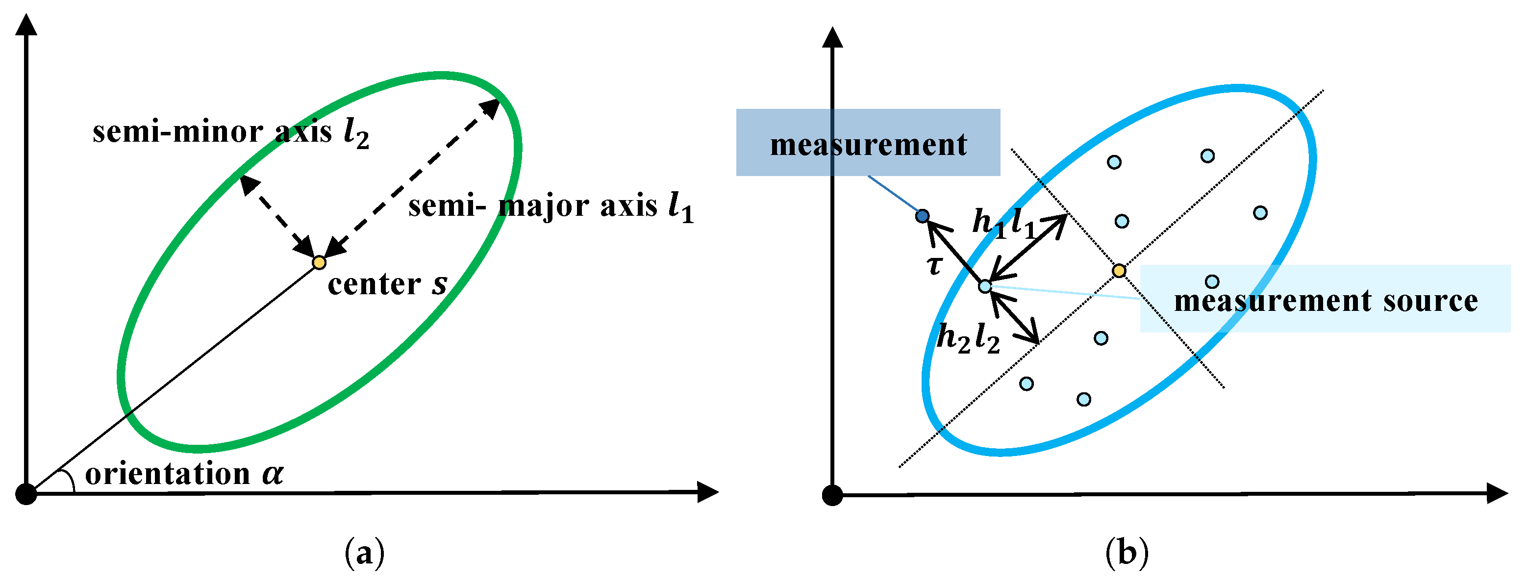
Figure 1. Illustration of the state parameterization and measurement model. (a) The state parameterization of a single target. (b) The measurement model of a single target.
Remotesensing 17 03696 g001
Figure 2. A schematic diagram of the processing flow in dense clutter. (Here, ‘Component’ is abbreviated as ‘Comp.’, and ‘Posterior Component’ is abbreviated as ‘PComp.’)
Remotesensing 17 03696 g002
Figure 3. The flowchart of the proposed method.
Remotesensing 17 03696 g003
Figure 4. Runtime comparison of the proposed method and the traditional ET-CPHD filter.
Remotesensing 17 03696 g004
Figure 5. Trajectories of four targets in Experiment 1. (The blue ‘×’ indicates the location of the launch point.)
Remotesensing 17 03696 g005
Figure 6. An example MC run of Experiment 1. (a) Period 1: From 1 s to 80 s, Tar. 1 and Tar. 2 approach and move parallel in the same direction at close range. (b) Period 2: From 81 s to 120 s, Tar. 1 and Tar. 2 end their parallel motion and merge, during which Tar. 3 and Tar. 4 appear and approach each other. (c) Period 3: From 121 s to 200 s, the merged target disappears, and Tar. 3 and Tar. 4 end their parallel motion and intersect.
Remotesensing 17 03696 g006
Figure 7. The GOSPA of Experiment 1.
Remotesensing 17 03696 g007
Figure 8. The estimated cardinality of Experiment 1.
Remotesensing 17 03696 g008
Figure 9. Schematic diagram of Experiment 2.
Remotesensing 17 03696 g009
Figure 10. Slices of selected frames of Experiment 2.
Remotesensing 17 03696 g010
Figure 11. The GOSPA of Experiment 2.
Remotesensing 17 03696 g011
Figure 12. The estimated cardinality of Experiment 2.
Remotesensing 17 03696 g012
Figure 13. A signalized intersection located in Chongqing.
Remotesensing 17 03696 g013
Figure 14. Trajectories of targets in Experiment 3.
Remotesensing 17 03696 g014
Figure 15. Estimation results for Experiment 3.
Remotesensing 17 03696 g015
Figure 16. The GOSPA of Experiment 3.
Remotesensing 17 03696 g016
Figure 17. The estimated cardinality of Experiment 3.
Remotesensing 17 03696 g017
Table 1. The hyperparameters in the VGMM.
ExplanationDefault Value
N emax Maximum number of executions for VGMM5
N rmax Maximum number of iterations per execution5
m k 0 j , β k 0 j Initial parameters of j-th Gaussian distribution m k 0 j = x ^ k | k 1 s j
β k 0 j = 1
ϵ k 0 j Initial parameters of j-th Dirichlet distribution ϵ k 0 j = 1
υ k 0 j , V k 0 j Initial parameters of j-th Wishart distribution υ k 0 j = 2 n d + 3
V k 0 j = S k | k 1 j S k | k 1 j T
Table 2. The number of targets at different time steps in Experiment 1.
Time step1s81 s101 s121 s176 s201 s
Number of targets
in scene
243220
SituationTar. 1 and
Tar. 2 birth
Tar. 3 and
Tar. 4 birth
Tar. 1 and
Tar. 2 merge
Merged target
dies
Tar. 3 and
Tar. 4 cross
Tar. 3 and
Tar. 4 die
Table 3. MTCE of the filters in simulation experiments.
Experiment 1Experiment 2
Target Count = 4Target Count = 4
MIS avg FAL avg MTCE MIS avg FAL avg MTCE
GIW-CPHD0.5120.0180.5300.1080.0040.112
MEM-CPHD0.6870.1230.8100.1000.0030.103
MEM-JIPDA0.0090.1390.1480.0110.0780.089
GIW-PMB0.4640.0120.4760.0830.0030.086
MEM-CPHD-VGMM0.0170.0090.0260.0060.0010.007
Table 4. The specific information of each target in Experiment 2.
ColorTypeSize
[ Length   ×   Width ]
Motion Time
[ Birth   Frame ,   Death   Frame ]
Initial State
[ s x ,   s y ,   s ˙ x ,   s ˙ y ]
Identifier
Dark blueTruck[8.10 × 2.50][1, 107][24, 87, 0, 8]Tar. 1
Light greenSaloon car[4.80 × 1.80][15, 101][35, 50, 0, 10]Tar. 2
OrangeSaloon car[4.80 × 1.80][9, 114][26, 50, 0, 10]Tar. 3
Light blueSaloon car[4.80 × 1.80][1, 111][25, 76, 0, 10]Tar. 4
Table 5. Runtime of the filters in simulation experiments.
Experiment 1Experiment 2
Target Count = 4,  ρ = 8.61 × 10 4 Target Count = 4,  ρ = 6.17 × 10 3
Single MCPer Iteration CycleSingle MCPer Iteration Cycle
GIW-CPHD170.800.854174.531.531
MEM-CPHD193.420.967190.841.674
MEM-JIPDA256.611.283230.052.018
GIW-PMB184.760.924185.771.630
MEM-CPHD-VGMM275.961.376241.342.117
Table 6. Average GOSPA ↓ of the filters under different parameter settings.
Experiment 1
Original Parameters:  P D = 0.98,  P S = 1,  λ C = 5,  Q a = 10 I 2
GIW-CPHDMEM-CPHDMEM-JIPDAGIW-PMBMEM-CPHD-VGMM
No change39.90136.19334.18537.19833.036
Q a = 2 Q a 40.30336.59435.37338.34533.284
Q a = 4 Q a 41.82439.20236.64239.11235.634
λ C = 4 λ C 42.66940.18538.78438.22437.332
λ C = 8 λ C 43.22542.18540.10541.87539.717
p D = 0.8 43.66540.37838.71840.48737.093
p D = 0.6 49.55647.09843.13746.51242.538
p S = 0.8 41.61239.63137.87539.14736.991
Experiment 2
Original Parameters:  P D = 0.98,  P S = 1,  λ C = 5,  Q a = 1.5 I 2
GIW-CPHDMEM-CPHDMEM-JIPDAGIW-PMBMEM-CPHD-VGMM
No change3.2712.5231.9362.7841.560
Q a = 2 Q a 4.0552.6692.6193.0151.577
Q a = 4 Q a 3.6322.8112.0973.2451.808
λ C = 4 λ C 3.7523.2102.6142.8322.108
λ C = 8 λ C 3.9513.5672.5143.1932.208
p D = 0.8 3.8642.9512.5973.0472.348
p D = 0.6 4.3573.4802.8393.2172.410
p S = 0.8 3.7453.1602.6212.9792.181
Table 7. MTCE of the filters in Experiment 3.
Experiment 3
Target Count = 3
GIW-CPHDMEM-CPHDMEM-JIPDAGIW-PMBMEM-CPHD-VGMM
MIS avg 0.8330.8110.0030.8070.002
FAL avg 0.3310.3240.0550.326 0.001
MTCE ↓1.1641.1350.0581.133 0.003
Table 8. Runtime of the filters in Experiment 3.
Experiment 3
Target Count = 3; Maximum Measurement Density:  6.5 × 10 3
GIW-CPHDMEM-CPHDMEM-JIPDAGIW-PMBMEM-CPHD-VGMM
Total runtime ↓49.0551.7553.3752.7455.17
Per iteration cycle ↓0.5450.5750.5930.5860.613
Disclaimer/Publisher’s Note: The statements, opinions and data contained in all publications are solely those of the individual author(s) and contributor(s) and not of MDPI and/or the editor(s). MDPI and/or the editor(s) disclaim responsibility for any injury to people or property resulting from any ideas, methods, instructions or products referred to in the content.