Author Contributions
Conceptualization, S.C. and Y.C.; methodology, Y.C.; software, Y.C.; validation, Y.C., S.C. and A.D.; resources, S.C.; data curation, Y.C.; writing—original draft preparation, Y.C.; Writing—review editing, Y.C.; visualization, Y.C.; supervision, S.C.; project administration, S.C.; funding acquisition, A.D. All authors have read and agreed to the published version of the manuscript.
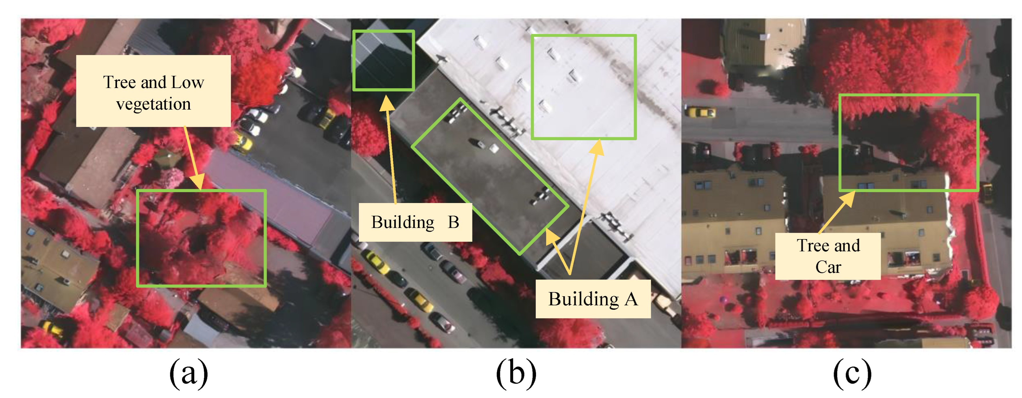
Figure 1.
Taking the ISPRS Vaihingen dataset as an example, the existing challenges in remote sensing semantic segmentation are demonstrated. (a) Trees and low shrubs have similar colors, making them difficult to distinguish. (b) The same building A appears differently in the image, while different buildings A and B belong to the same category but exhibit distinct visual characteristics. (c) The object boundaries in the image are complex and intertwined, with shadow occlusion issues also present.
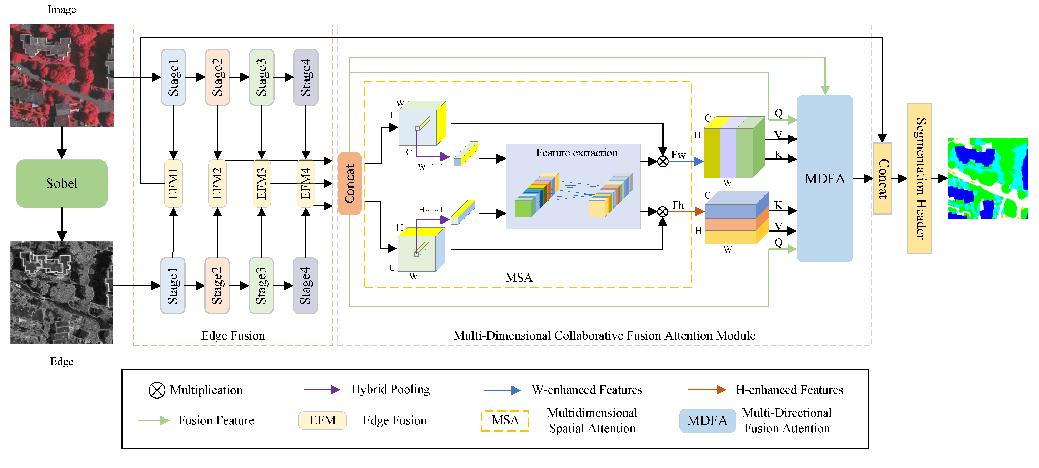
Figure 2.
The first stage is spatial feature extraction. Subsequently, the second stage performs various feature enhancement and fusion, including horizontal-vertical feature enhancement and fusion attention. Specifically, horizontal-vertical feature enhancement extracts image feature information from different dimensions, while fusion attention integrates information from various dimensions to achieve fusion of both global and local information.
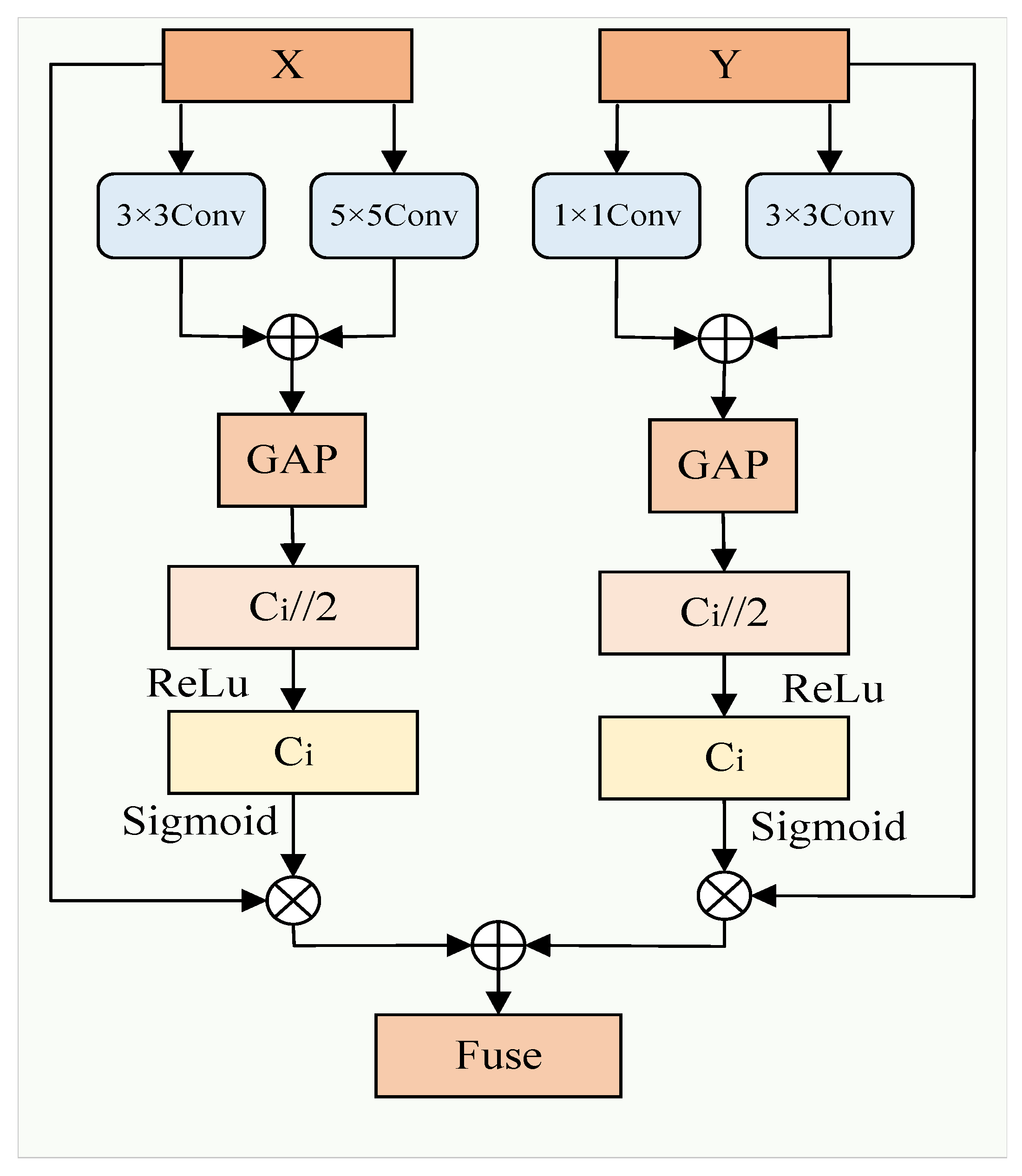
Figure 3.
The proposed EFM module is used to fuse the edge branch with the original encoder branch features. It consists of two branches for channel enhancement, and finally, the information from both branches is fused by addition.
Figure 3.
The proposed EFM module is used to fuse the edge branch with the original encoder branch features. It consists of two branches for channel enhancement, and finally, the information from both branches is fused by addition.
Figure 4.
The proposed MSA improvement module enhances the input data by swapping dimensions to strengthen the corresponding horizontal and vertical features. After pooling, the features are fused through a convolution and a linear layer, ultimately producing the enhanced output, and N represents the corresponding enhanced dimension.
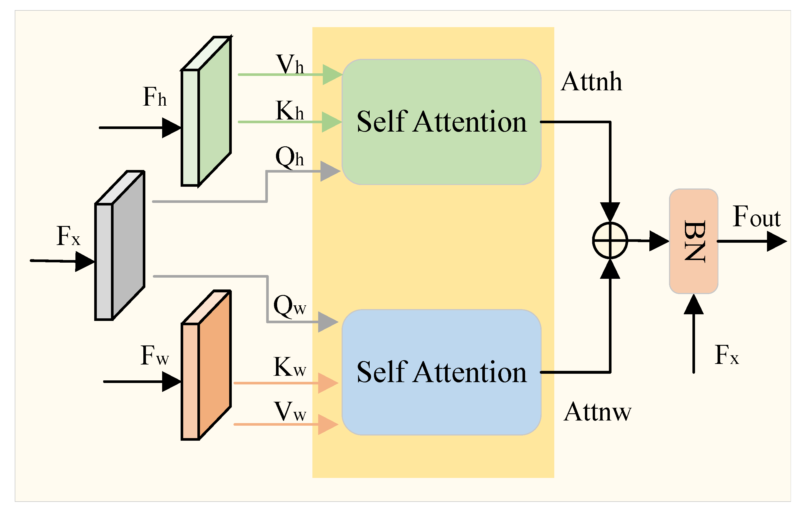
Figure 5.
The proposed MDFA module integrates the fused query with the edge-enhanced vertical and horizontal key-value pairs, effectively capturing boundary-aware spatial dependencies and enhancing feature representation in remote sensing segmentation.
Figure 5.
The proposed MDFA module integrates the fused query with the edge-enhanced vertical and horizontal key-value pairs, effectively capturing boundary-aware spatial dependencies and enhancing feature representation in remote sensing segmentation.
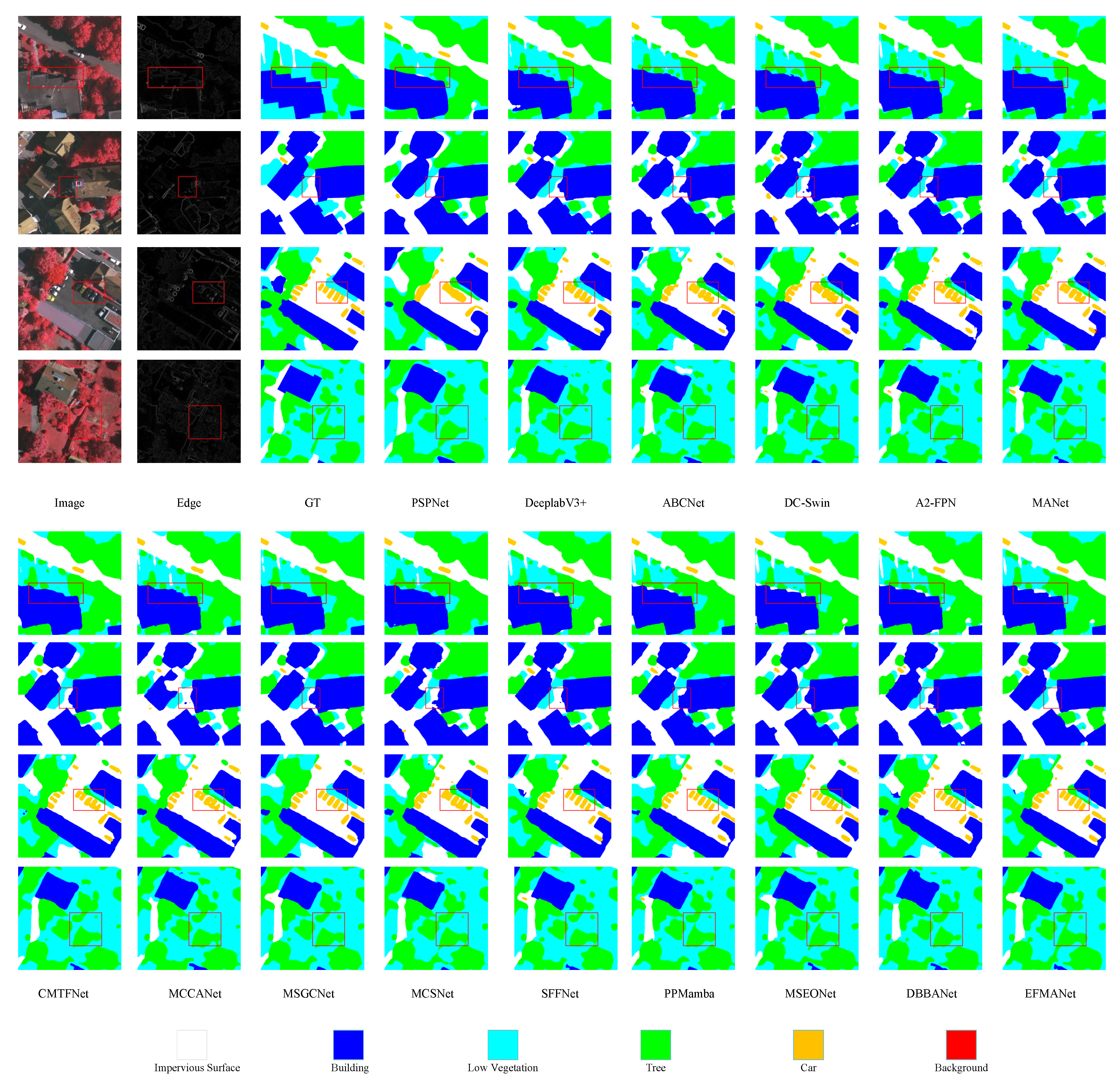
Figure 6.
The visualized comparative results on the Vaihingen dataset. The red square indicates the area that requires attention for comparison.
Figure 6.
The visualized comparative results on the Vaihingen dataset. The red square indicates the area that requires attention for comparison.
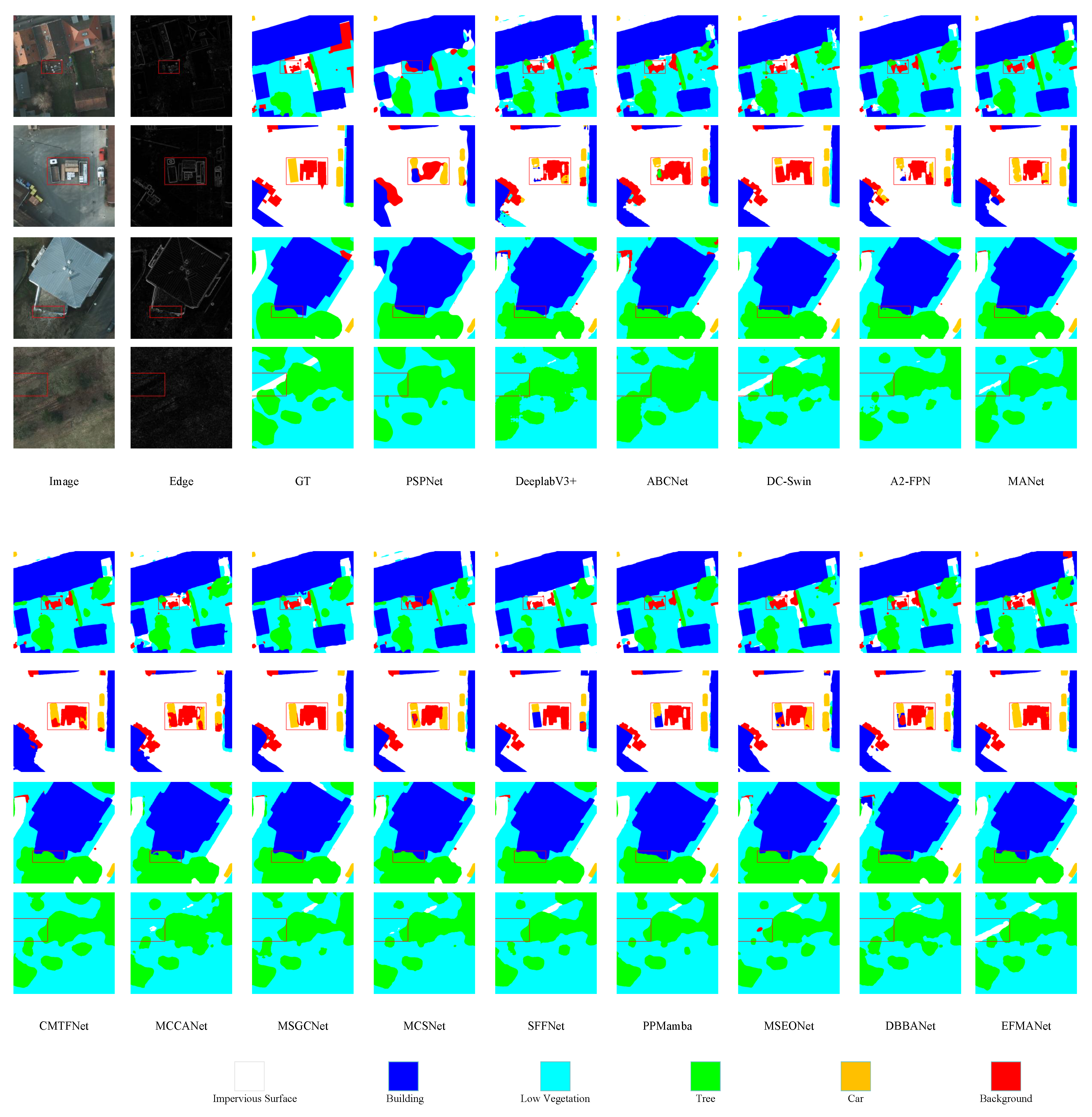
Figure 7.
The visualized comparative results on the Potsdam dataset. The red square indicates the area that requires attention for comparison.
Figure 7.
The visualized comparative results on the Potsdam dataset. The red square indicates the area that requires attention for comparison.
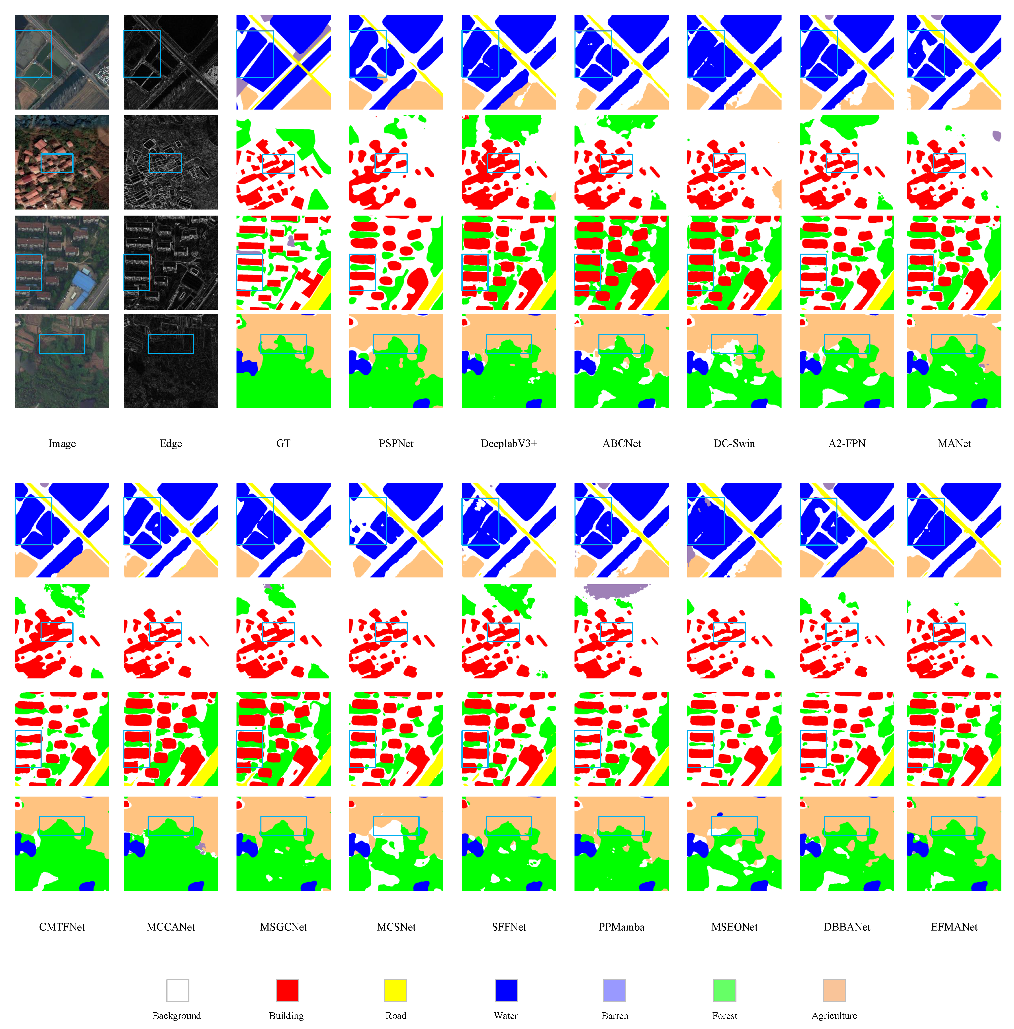
Figure 8.
The visualized comparative results on the LoveDA dataset. The blue square indicates the area that requires attention for comparison.
Figure 8.
The visualized comparative results on the LoveDA dataset. The blue square indicates the area that requires attention for comparison.
Figure 9.
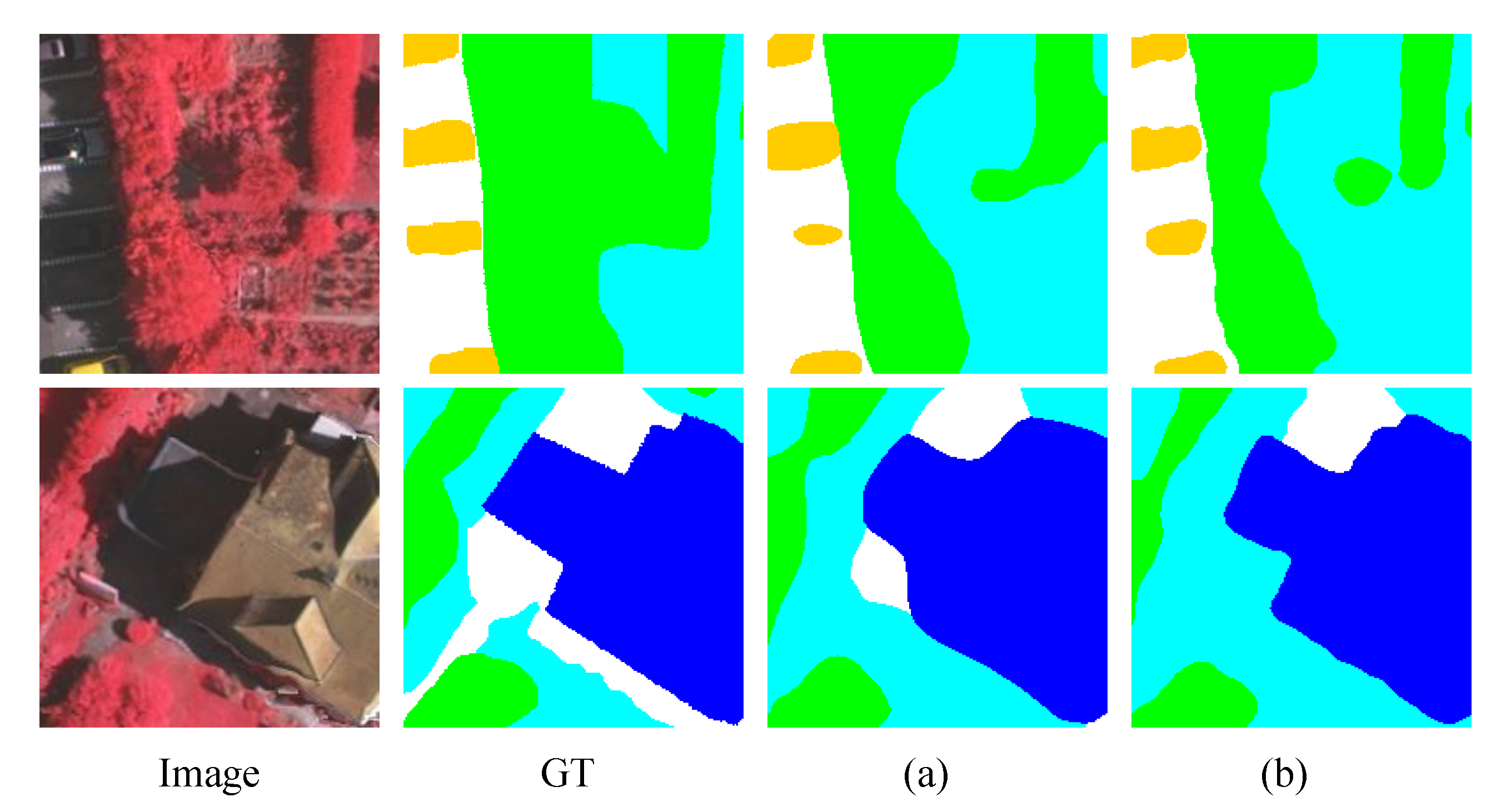
Enlarged segmentation results before and after adding EFM in the Baseline. (a) Baseline (b) Baseline + EFM. These results demonstrate that the incorporation of the EFM module significantly enhances the accuracy of object recognition, particularly in challenging regions such as complex object boundaries and small objects affected by shadows or occlusions.
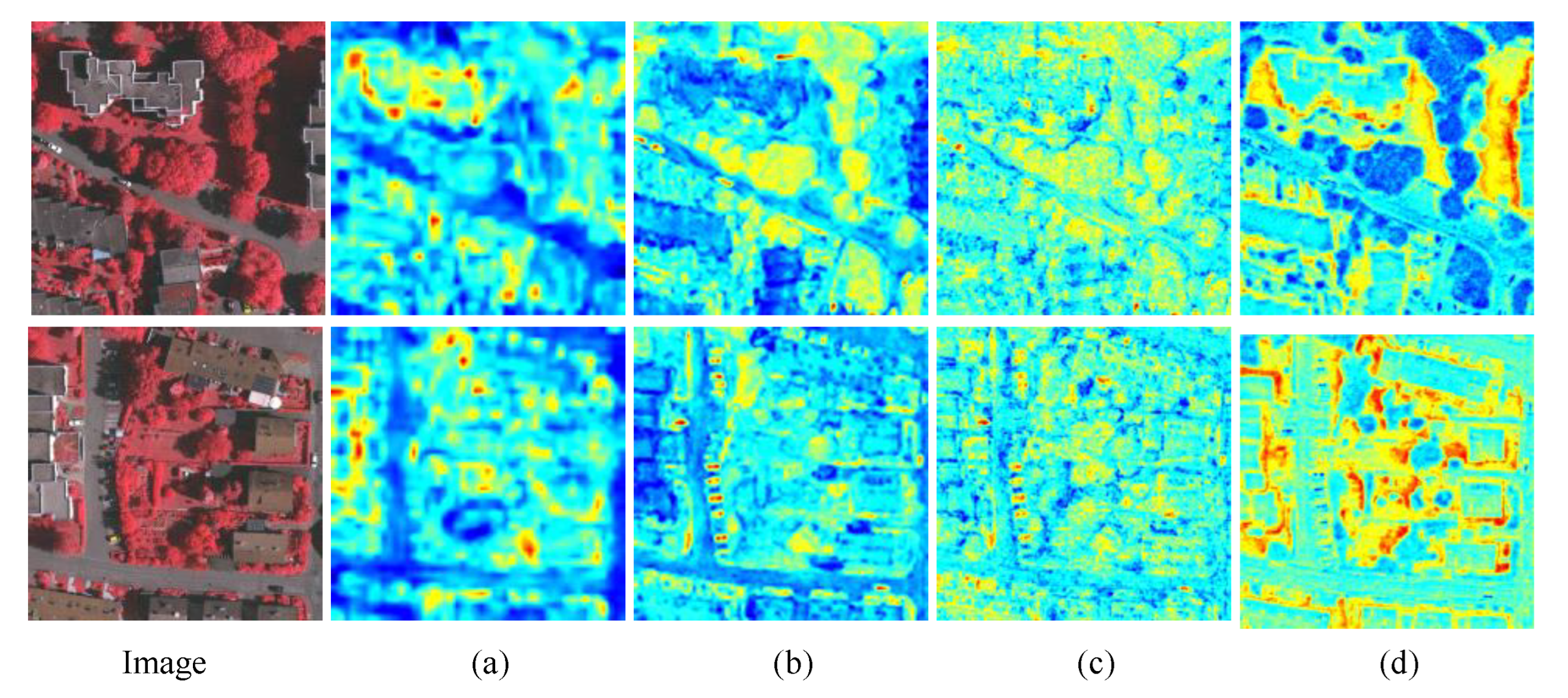
Figure 10.
Heatmaps of each stage module. (a) Features output by the Baseline after passing through the encoder. (b) Fusion features of the encoder after incorporating the EFM module. (c) Output features after integrating the MSA module. (d) Features output after applying the MDFA module. The results suggest that the introduction of edge information enables the model to better focus on fine-scale objects, complex object boundaries, and targets in shadowed regions. In addition, the incorporation of spatial attention guides the model to capture the overall structural layout more effectively.
Figure 11.
Enlarged segmentation results before and after adding MCFA in the Baseline. (a) Baseline (b) Baseline + MCFA. The results indicate that the use of the MCFA module, which integrates both global and local contextual information, leads to more accurate recognition of both large-scale and small-scale objects.
Figure 12.
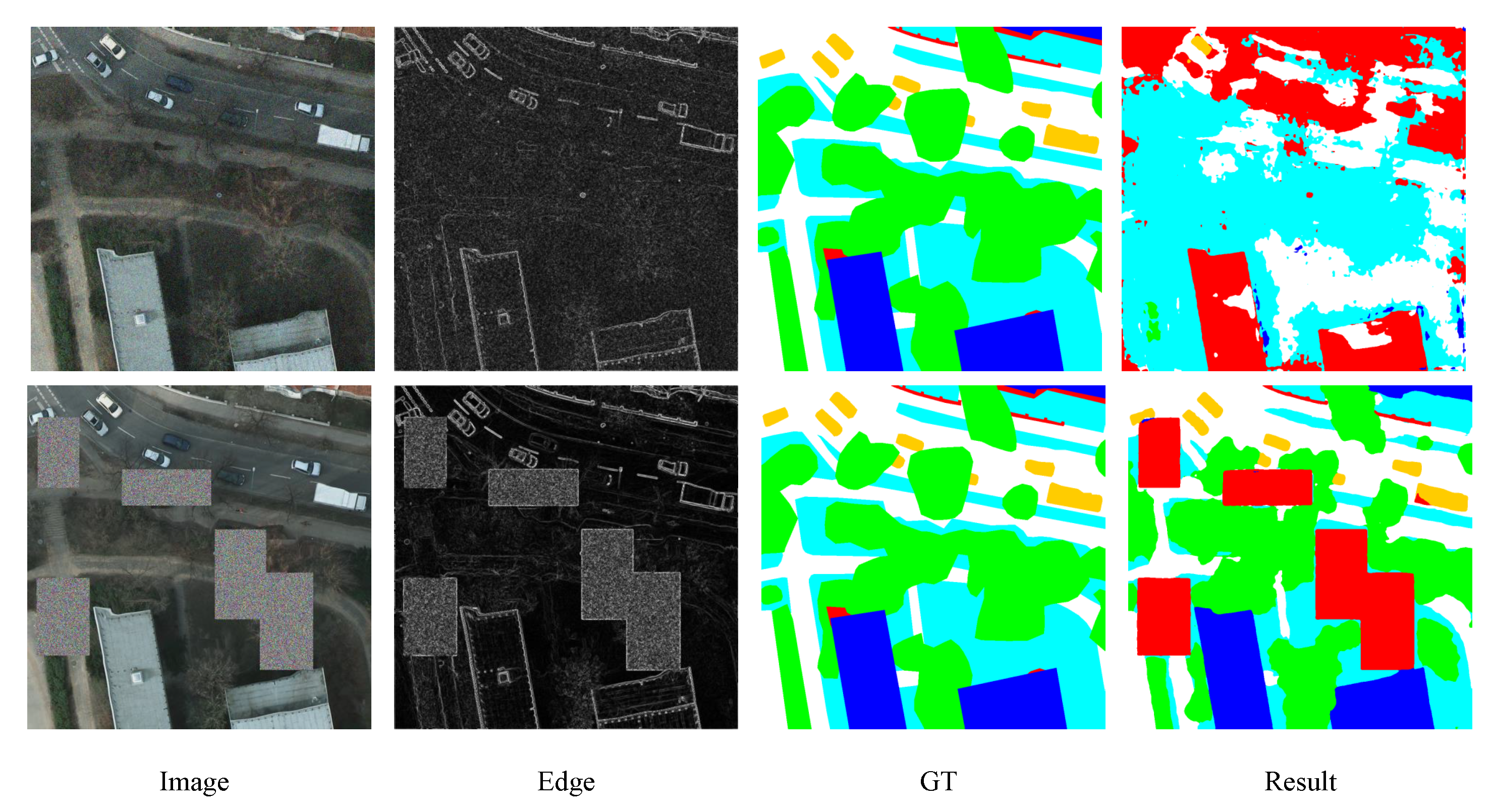
The image shows the prediction results under conditions of extreme noise and partial occlusion.
Figure 12.
The image shows the prediction results under conditions of extreme noise and partial occlusion.
Table 1.
Comparative experiments on Vaihingen Dataset.
Table 1.
Comparative experiments on Vaihingen Dataset.
| Method | F1 (%) | Evaluation Index |
|---|
| Imp.Surf. | Building | Lowveg. | Tree | Car | Mean F1 (%) | OA (%) | mIoU (%) |
|---|
| PSPNet [34] | 95.67 | 93.22 | 83.11 | 88.78 | 77.41 | 87.64 | 91.66 | 78.62 |
| DeeplabV3+ [35] | 96.58 | 95.27 | 84.15 | 89.76 | 85.19 | 90.19 | 92.96 | 82.53 |
| ABCNet [36] | 96.45 | 94.81 | 84.16 | 90.19 | 83.97 | 89.92 | 92.79 | 82.08 |
| DC-Swin [37] | 96.96 | 96.09 | 84.85 | 90.24 | 86.83 | 90.99 | 93.51 | 83.84 |
| -FPN [38] | 96.78 | 95.56 | 84.63 | 90.08 | 88.47 | 91.10 | 93.26 | 83.99 |
| MANet [39] | 96.74 | 95.47 | 84.61 | 89.73 | 88.75 | 91.06 | 93.07 | 83.89 |
| CMTFNet [32] | 96.99 | 95.98 | 85.31 | 90.40 | 87.21 | 91.18 | 93.61 | 84.12 |
| MCCANet [40] | 96.31 | 94.41 | 84.20 | 89.96 | 83.93 | 89.76 | 92.68 | 81.81 |
| MSGCNet [33] | 96.86 | 95.86 | 85.45 | 90.57 | 89.63 | 91.67 | 93.60 | 84.90 |
| MCSNet [41] | 97.00 | 95.54 | 84.41 | 90.37 | 88.21 | 91.19 | 93.45 | 84.12 |
| SFFNet [42] | 97.06 | 95.75 | 85.06 | 90.14 | 90.33 | 91.67 | 93.51 | 84.91 |
| PPMamba [43] | 97.00 | 96.08 | 85.54 | 90.48 | 88.77 | 91.57 | 93.68 | 84.76 |
| MSEONet [16] | 96.78 | 95.75 | 84.48 | 90.16 | 88.22 | 91.08 | 93.26 | 83.95 |
| DBBANet [31] | 96.77 | 95.40 | 84.96 | 90.32 | 89.12 | 91.30 | 93.29 | 84.31 |
| EFMANet | 97.20 | 96.13 | 86.21 | 91.06 | 90.79 | 92.28 | 94.00 | 85.92 |
Table 2.
Comparative experiments on Potsdam Dataset.
Table 2.
Comparative experiments on Potsdam Dataset.
| Method | F1 (%) | Evaluation Index |
|---|
| Imp.Surf. | Building | Lowveg. | Tree | Car | Mean F1 (%) | OA (%) | mIoU (%) |
|---|
| PSPNet [34] | 91.31 | 92.70 | 83.65 | 82.41 | 91.82 | 88.38 | 87.30 | 79.45 |
| DeeplabV3+ [35] | 93.85 | 96.20 | 87.20 | 88.79 | 95.83 | 92.37 | 91.16 | 86.04 |
| ABCNet [36] | 93.36 | 96.47 | 86.76 | 88.64 | 95.98 | 92.24 | 90.71 | 85.84 |
| DC-Swin [37] | 94.33 | 96.94 | 87.97 | 89.38 | 86.31 | 92.99 | 91.78 | 87.11 |
| -FPN [38] | 93.97 | 96.31 | 87.49 | 88.61 | 96.22 | 92.53 | 91.32 | 86.33 |
| MANet [39] | 93.78 | 96.44 | 87.63 | 89.16 | 96.41 | 92.69 | 91.42 | 86.59 |
| CMTFNet [32] | 94.58 | 97.01 | 88.24 | 89.22 | 96.24 | 93.06 | 91.96 | 87.25 |
| MCCANet [40] | 93.54 | 96.10 | 87.00 | 88.17 | 95.33 | 92.03 | 90.72 | 85.45 |
| MSGCNet [33] | 94.43 | 96.92 | 87.75 | 89.10 | 96.59 | 92.96 | 91.80 | 87.08 |
| MCSNet [41] | 94.11 | 96.64 | 87.72 | 88.82 | 95.79 | 92.62 | 91.44 | 86.46 |
| SFFNet [42] | 94.62 | 96.90 | 88.24 | 89.22 | 96.93 | 93.18 | 91.97 | 87.47 |
| PPMamba [43] | 94.54 | 96.95 | 88.29 | 89.48 | 96.47 | 93.15 | 92.07 | 87.38 |
| MSEONet [16] | 94.32 | 97.05 | 87.77 | 89.00 | 96.22 | 92.87 | 91.56 | 86.93 |
| DBBANet [31] | 94.24 | 96.55 | 87.68 | 88.92 | 96.46 | 92.77 | 91.49 | 86.74 |
| EFMANet (ours) | 94.96 | 97.34 | 88.55 | 89.86 | 96.87 | 93.52 | 92.53 | 88.03 |
Table 3.
Comparative experiments on LoveDA Dataset.
Table 3.
Comparative experiments on LoveDA Dataset.
| Method | Background | Building | Road | Water | Barren | Forest | Agriculture | mIoU |
|---|
| PSPNet [34] | 40.98 | 47.40 | 45.92 | 75.23 | 10.69 | 40.44 | 56.30 | 45.28 |
| DeeplabV3+ [35] | 53.41 | 58.61 | 54.61 | 69.28 | 28.55 | 43.11 | 52.07 | 51.27 |
| ABCNet [36] | 41.15 | 55.01 | 49.71 | 77.61 | 15.26 | 44.41 | 54.19 | 48.19 |
| DC-Swin [37] | 53.47 | 61.43 | 55.47 | 70.27 | 32.45 | 44.06 | 58.29 | 52.86 |
| -FPN [38] | 43.46 | 57.02 | 52.63 | 76.53 | 17.85 | 45.06 | 56.63 | 49.88 |
| MANet [39] | 46.63 | 54.18 | 53.56 | 83.81 | 15.07 | 45.00 | 51.51 | 49.97 |
| CMTFNet [32] | 45.47 | 56.85 | 60.20 | 78.43 | 18.67 | 47.31 | 57.34 | 52.04 |
| MCCANet [40] | 40.80 | 52.92 | 52.98 | 77.09 | 16.81 | 41.32 | 54.72 | 48.90 |
| MSGCNet [33] | 52.54 | 57.71 | 57.93 | 80.03 | 16.44 | 46.23 | 59.07 | 51.42 |
| MCSNet [41] | 45.14 | 61.77 | 58.12 | 82.10 | 17.38 | 47.15 | 61.36 | 53.29 |
| SFFNet [42] | 54.37 | 64.22 | 56.56 | 68.67 | 32.95 | 44.66 | 52.02 | 53.35 |
| PPMamba [43] | 54.15 | 63.28 | 55.25 | 68.36 | 34.96 | 40.86 | 51.30 | 52.59 |
| MSEONet [16] | 45.22 | 55.22 | 53.72 | 78.45 | 15.65 | 46.50 | 59.84 | 50.66 |
| DBBANet [31] | 45.21 | 55.40 | 53.04 | 77.81 | 15.17 | 45.26 | 57.75 | 49.95 |
| EFMANet (ours) | 47.25 | 60.89 | 58.43 | 81.66 | 18.36 | 49.25 | 56.48 | 54.48 |
Table 4.
McNemar Test Results on the Vaihingen and Potsdam Datasets for Recent Semantic Segmentation Networks.
Table 4.
McNemar Test Results on the Vaihingen and Potsdam Datasets for Recent Semantic Segmentation Networks.
| Network | Vaihingen | Potsdam |
|---|
| B () | C () | () | p | B () | C () | () | p |
|---|
| PSPNet [34] | 4.73 | 2.468 | 0.711 | <0.001 | 40.837 | 13.515 | 13.735 | <0.001 |
| DeeplabV3+ [35] | 2.691 | 2.112 | 0.070 | <0.001 | 19.720 | 10.976 | 2.491 | <0.001 |
| ABCNet [36] | 3.707 | 2.257 | 0.352 | <0.001 | 19.822 | 10.959 | 2.552 | <0.001 |
| DC-Swin [37] | 2.376 | 2.071 | 0.021 | <0.001 | 12.545 | 10.799 | 0.131 | <0.001 |
| -FPN [38] | 2.777 | 1.968 | 0.138 | <0.001 | 16.621 | 11.186 | 1.062 | <0.001 |
| MANet [39] | 3.534 | 2.495 | 0.179 | <0.001 | 15.007 | 10.565 | 0.772 | <0.001 |
| CMTFNet [32] | 2.331 | 1.916 | 0.041 | <0.001 | 13.210 | 11.504 | 0.118 | <0.001 |
| MCCANet [40] | 3.655 | 2.187 | 0.369 | <0.001 | 19.281 | 10.770 | 2.411 | <0.001 |
| MSGCNet [33] | 2.145 | 1.983 | 0.006 | <0.001 | 13.704 | 11.141 | 0.264 | <0.001 |
| MCSNet [41] | 2.639 | 2.057 | 0.072 | <0.001 | 15.935 | 11.355 | 0.769 | <0.001 |
| SFFNet [42] | 2.140 | 1.721 | 0.045 | <0.001 | 11.627 | 10.313 | 0.079 | <0.001 |
| PPMamba [43] | 2.100 | 1.871 | 0.013 | <0.001 | 12.159 | 11.185 | 0.041 | <0.001 |
| MSEONet [16] | 2.619 | 1.821 | 0.143 | <0.001 | 13.555 | 9.700 | 0.639 | <0.001 |
| DBBANet [31] | 2.506 | 1.812 | 0.111 | <0.001 | 13.860 | 10.010 | 0.621 | <0.001 |
| EFMANet (ours) | 1.987 | 1.654 | 0.008 | <0.001 | 10.524 | 9.412 | 0.036 | <0.001 |
Table 5.
Ablation Experiments on the Vaihingen and Potsdam Datasets.
Table 5.
Ablation Experiments on the Vaihingen and Potsdam Datasets.
| Method | Vaihingen | Potsdam |
|---|
| mIoU (%) | F1 (%) | mIoU (%) | F1 (%) |
|---|
| EFMANet | 85.92 | 92.28 | 88.03 | 93.52 |
| EFMANet w/o EFM | 85.15 | 91.81 | 87.04 | 92.95 |
| EFMANet w/o MCFA | 85.04 | 91.73 | 87.11 | 92.99 |
| EFMANet w/o MCFA-H | 85.15 | 91.80 | 87.25 | 93.07 |
| EFMANet w/o MCFA-W | 85.25 | 91.86 | 87.16 | 93.03 |
| EFMANet w/o MDFA | 85.48 | 92.01 | 87.51 | 93.23 |
Table 6.
Results of adding individual models on baseline model on vaihingen dataset.
Table 6.
Results of adding individual models on baseline model on vaihingen dataset.
| Method | F1 (%) | Evaluation Index |
|---|
| Imp.Surf. | Building | Lowveg. | Tree | Car | Mean F1 (%) | OA (%) | mIoU (%) |
|---|
| Baseline | 96.52 | 95.39 | 84.14 | 90.06 | 81.63 | 89.55 | 93.00 | 81.59 |
| Baseline + EFM | 96.69 | 95.80 | 84.98 | 90.29 | 83.18 | 90.19 | 93.32 | 82.58 |
| Baseline + MCFA | 96.64 | 95.57 | 84.70 | 90.09 | 82.99 | 90.00 | 93.16 | 82.28 |
| Baseline + MCFA-H | 96.56 | 95.47 | 84.72 | 90.22 | 81.89 | 89.77 | 93.14 | 81.94 |
| Baseline + MCFA-W | 96.59 | 95.52 | 84.71 | 90.17 | 82.12 | 89.82 | 93.15 | 82.02 |
Table 7.
Comparison of different edge detection methods on segmentation performance.
Table 7.
Comparison of different edge detection methods on segmentation performance.
| Method | mIoU (%) | OA (%) | F1 (%) |
|---|
| Laplacian | 85.43 | 93.78 | 91.92 |
| Canny | 85.85 | 93.99 | 92.20 |
| Sobel (ours) | 85.92 | 94.00 | 92.28 |
Table 8.
Results of adding EFM on baseline model on Vaihingen Dataset. × indicates that the layer is not used, and ✓ indicates that the EFM of this layer is used.
Table 8.
Results of adding EFM on baseline model on Vaihingen Dataset. × indicates that the layer is not used, and ✓ indicates that the EFM of this layer is used.
| EFM Modules | F1 (%) | Evaluation Index |
|---|
| EFM1 | EFM2 | EFM3 | EFM4 | Imp.Surf. | Building | Lowveg. | Tree | Car | Mean F1 (%) | OA (%) | mIoU (%) |
|---|
| × | × | × | × | 96.52 | 95.39 | 84.14 | 90.06 | 81.63 | 89.55 | 93.00 | 81.59 |
| ✓ | × | × | × | 96.73 | 95.79 | 83.55 | 90.00 | 86.12 | 90.43 | 93.13 | 82.96 |
| ✓ | ✓ | × | × | 97.03 | 95.74 | 83.49 | 89.92 | 89.07 | 91.05 | 93.24 | 83.94 |
| ✓ | ✓ | ✓ | × | 97.09 | 95.96 | 83.56 | 90.02 | 90.05 | 91.34 | 93.35 | 84.41 |
| ✓ | ✓ | ✓ | ✓ | 97.12 | 96.06 | 85.59 | 90.72 | 89.29 | 91.74 | 93.78 | 85.04 |
Table 9.
Comparison of different Attention modules on Vaihingen Dataset.
Table 9.
Comparison of different Attention modules on Vaihingen Dataset.
| Method | F1 (%) | Evaluation Index |
|---|
| Imp.Surf. | Building | Lowveg. | Tree | Car | Mean F1 | OA | mIoU |
|---|
| Baseline | 90.12 | 92.45 | 82.36 | 87.29 | 76.14 | 89.55 | 89.32 | 81.59 |
| Baseline + ECA-CA | 96.52 | 95.44 | 84.51 | 89.99 | 82.71 | 89.83 | 93.04 | 82.01 |
| Baseline + SE | 96.62 | 95.56 | 84.83 | 89.83 | 82.47 | 89.86 | 93.09 | 82.07 |
| Baseline + CA | 96.64 | 95.56 | 84.72 | 89.99 | 82.49 | 89.88 | 93.14 | 82.10 |
| Baseline + MSA (ours) | 90.73 | 92.89 | 83.19 | 87.88 | 78.05 | 90.00 | 89.81 | 82.28 |
Table 10.
Comparison of MDFA concatenation and pixel-wise addition for feature fusion on Potsdam dataset.
Table 10.
Comparison of MDFA concatenation and pixel-wise addition for feature fusion on Potsdam dataset.
| Method | mIoU (%) | OA (%) | F1 (%) | Imp.Surf. | Building | Lowveg. | Tree | Car |
|---|
| MDFA-concat | 75.75 | 89.41 | 85.90 | 94.58 | 88.89 | 78.66 | 87.53 | 79.78 |
| MDFA-pixel add (ours) | 85.92 | 94.00 | 92.28 | 97.20 | 96.13 | 86.21 | 91.06 | 90.79 |
Table 11.
Comparison of parameters and mIoU of different backbone on Vaihingen Dataset.
Table 11.
Comparison of parameters and mIoU of different backbone on Vaihingen Dataset.
| Backbone | Params (M) | mIoU (%) |
|---|
| Resnet18 | 15.6 | 84.65 |
| Resnext50 | 104.0 | 84.44 |
| Convnext-Tiny | 39.9 | 85.34 |
| Convnext-Small | 63.9 | 85.92 |
Table 12.
Comparison of Single-Branch Network and EFMANet in terms of segmentation performance and computational cost.
Table 12.
Comparison of Single-Branch Network and EFMANet in terms of segmentation performance and computational cost.
| Method | mIoU (%) | F1 (%) | Params (M) | FLOPs (G) |
|---|
| Single-Branch | 85.15 | 91.81 | 58.20 | 50.18 |
| EFMANet (Dual-Branch) | 85.92 | 92.28 | 63.90 | 74.40 |
Table 13.
Comparison of parameters and computation of different networks.
Table 13.
Comparison of parameters and computation of different networks.
| Method | Params (M) | Flops (G) |
|---|
| PSPNet [34] | 53.3 M | 28.1 G |
| DeeplabV3+ [35] | 40.3 M | 138.6 G |
| ABCNet [36] | 13.6 M | 15.7 G |
| DC-Swin [37] | 66.9 M | 72.1 G |
| -FPN [38] | 22.8 M | 41.7 G |
| MANet [39] | 35.9 M | 54.2 G |
| CMTFNet [32] | 30.1 M | 34.3 G |
| MCCANet [40] | 43.0 M | 65.1 G |
| MSGCNet [33] | 27.6 M | 29.1 G |
| MCSNet [41] | 54.7 M | 63.9 G |
| SFFNet [42] | 34.1 M | 52.0 G |
| PPMamba [43] | 21.7 M | 23.1 G |
| MSEONet [16] | 47.19 M | 45.25 G |
| DBBANet [31] | 36.00 M | 62.78 G |
| EFMANet (ours) | 63.9 M | 74.4 G |
