Satellite-Based Machine Learning for Soil Moisture Prediction and Land Conservation Practice Assessment in West African Drylands

Highlights

What are the main findings?

• Integration of SMAP, Sentinel-2, and WaPOR data through LSTM modeling enabled accurate daily soil moisture prediction across fragmented smallholder landscapes in semiarid northern Ghana.
• Stone bunds presented consistent soil moisture enhancement across multiple years, terrain types, and seasons, with benefits most pronounced on steeper slopes and in areas with lower topographic wetness.

What is the implication of the main findings?

• The modeling framework provides a transferable approach for monitoring soil–water dynamics in data-sparse dryland regions where traditional monitoring infrastructure is absent.
• Model-enhanced satellite observations of soil moisture enable quantification of conservation practice effectiveness, supporting evidence-driven scaling of nature-based solutions for climate adaptation in vulnerable agricultural systems.

Abstract

In semiarid, fragmented landscapes where data scarcity challenges effective land management, accurate soil moisture monitoring is critical. This study presents a high-resolution analysis that integrates remote sensing, in situ data, and machine learning to predict soil moisture and evaluate the impact of land conservation practices. A Long Short-Term Memory (LSTM) model combined with Random Forest gap-filling achieved strong predictive performance (R² = 0.84; RMSE = 0.103 cm³ cm⁻³), outperforming SMAP satellite estimates by approximately 30% across key accuracy metrics. The model was applied to 222 field sites in northern Ghana to quantify the effects of stone bunds on soil moisture retention. The results revealed that fields with stone bunds maintained 4–6% higher moisture than non-bunded fields, particularly on steep slopes and in areas with low to moderate topographic wetness. These findings demonstrate the capability of combining remote sensing and deep learning for fine-scale soil-moisture prediction and provide quantitative evidence of how nature-based solutions enhance water retention and climate resilience in dryland agricultural systems.

1. Introduction

Soil moisture is a critical component of the Earth’s hydrological cycle and significantly influences various environmental and agricultural processes [1,2] Accurately capturing the spatiotemporal dynamics of soil moisture is essential for applications ranging from local-scale field management to large-scale hydrological modeling. These applications include short-term weather forecasting [3], drought monitoring [4,5], modeling catchment hydrologic responses [6], and understanding ecological processes and spatial patterns [7,8]. In semiarid regions such as West Africa, where agriculture is predominantly rain-fed, knowledge of soil moisture variability is especially important for evaluating crop productivity, drought preparedness, and sustainable water resource management [9,10]. However, erratic rainfall and limited access to soil moisture data complicate agricultural planning, leaving farmers and decision-makers with insufficient information, resulting in missed opportunities for environmental mitigation [11,12,13]. Continuous soil moisture monitoring is therefore critical not only to reduce environmental risks but also to increase crop resilience and support food security under increasingly variable climatic conditions.

Accurate estimation of soil moisture across diverse landscapes is challenging due to spatial variability driven by heterogeneities in soil properties, topography, and vegetation cover [14]. Current approaches include in situ measurements, remote sensing, and modeling techniques [6,15,16,17], each with distinct advantages and limitations that vary according to spatial and temporal application scales. In situ measurements provide high precision but suffer from sparse spatial distribution, limiting their utility for regional or large-scale assessments [11]. While dense ground-based sensor networks could address coverage limitations, deployment costs are impractical in resource-constrianed regions [18]. Satellite remote sensing offers broad spatial coverage and frequent temporal observations, yet coarse spatial resolution and temporal gaps limit its applicability in smallholder agricultural systems [19,20]. Physically based models can generate continuous global soil moisture estimates but often have high uncertainty due to nonlinear interactions among soil, vegetation, and atmospheric variables [14]. These limitations are particularly pronounced in West Africa, where the absence of high-resolution, continuous soil moisture data constrains timely interventions and the implementation of sustainable land management practices [21].

Among the strategies used to increase soil moisture retention and mitigate land degradation in drylands, soil and water conservation practices such as stone bunds play a key role. Stone bunding, a traditional technique widely practiced in northern Ghana, involves placing stones along contour lines to slow runoff, reduce soil erosion, and increase infiltration [22,23,24,25,26]. Although several plot-scale studies have demonstrated the effectiveness of stone bunds [24,27], their landscape-level hydrological impact is poorly quantified, especially in agroecosystems where microclimatic and topographic heterogeneity creates complex moisture dynamics beyond the resolution of conventional monitoring approaches. Evaluating the effectiveness of conservation measures at the landscape scale requires spatially continuous and temporally resolved soil moisture data, a requirement that is rarely met in low-resource, semiarid settings [14,28,29,30,31].

Recent research has highlighted the growing need for high-resolution soil moisture estimates that can accurately represent the complex interactions between hydrological and ecological processes at multiple scales [32,33]. Machine learning techniques offer the potential to address this challenge by integrating multisource satellite observations with environmental data to capture nonlinear relationships and generate improved spatial and temporal resolutions [14,34,35]. Therefore, this study integrates Random Forest (RF) and Long Short-Term Memory (LSTM) networks to predict daily soil moisture dynamics and evaluate stone-bund effectiveness in northern Ghana. Random forest models excel at processing high-dimensional, nonlinear features for spatial and temporal downscaling without requiring strict distributional assumptions [36,37]. LSTM networks capture both short- and long-term temporal dependencies in sequential environmental data, enabling accurate time series prediction [38,39]. We combine SMAP-derived soil moisture, Normalized Difference Vegetation Index (NDVI), Actual Evapotranspiration Index (AETI), and environmental variables with field measurements as follows:

(i)

Generate daily soil moisture predictions via LSTM networks trained on spatially downscaled remote sensing inputs;

(ii)

Fine-scale spatial heterogeneity in soil moisture across fragmented, semiarid landscapes is captured;

(iii)

Quantify the spatiotemporal impacts of stone bunds on soil moisture retention across 222 field sites in northern Ghana.

This approach advances both computational capabilities and practical applications for sustainable land management in data-limited dryland environments.

2. Materials and Methods

2.1. Study Area

This study was conducted in the Nandom District, located in the Upper West Region of Ghana, covering approximately 391 km² between latitudes 10°40′–11°00′N and longitudes 2°25′–2°45′W (Figure 1). The area lies within the Guinea Savannah ecological zone, characterized by gently undulating topography, scattered trees, and mixed croplands. The elevation ranges from 210 to 280 m above sea level, with slopes varying between 0 and 12%, creating subtle microtopographic differences that influence runoff and infiltration.

The district experiences a semiarid tropical climate, with a single rainy season (May–October) and a dry season (November–April). Mean annual rainfall is 800–1100 mm, while mean daily temperature ranges between 25 °C and 35 °C. These conditions pose challenges for soil moisture retention, drought resilience, and rainfed crop production. The predominant land uses are smallholder rainfed agriculture and fallow vegetation, with sorghum, millet, maize, and groundnut as the main crops, interspersed with scattered trees such as Vitellaria paradoxa (shea) and Parkia biglobosa (locust bean). These land uses directly affect evapotranspiration and soil moisture variability across the landscape.

There are two categories of agricultural fields in the study area:

• Stone-bunded fields (S): plots bordered by contour-aligned stone bunds designed to reduce runoff and enhance infiltration.
• Non-bunded fields (N): adjacent or nearby control plots lacking physical soil and water conservation structures.

The classification was initially performed using high-resolution Google Earth imagery and verified through field surveys conducted between 2019 and 2024. A total of 222 fields were mapped, consisting of 100S and 122N sites, representing approximately 45% and 55%, respectively, of the total surveyed area.

Field selection followed a stratified sampling approach for a balanced representation across slope, elevation, and management categories. Specifically, stone-bunded and non-bunded fields were selected in paired proximity (<300 m) to minimize differences in soil type and rainfall exposure. The coordinates of each site were recorded using a Garmin GPSMAP 64s (Garmin Ltd., Olathe, KS, USA), enabling precise spatial mapping and integration with remotely sensed datasets.

2.2. Data

2.2.1. Ground-Based Data: In Situ Measurements

In situ soil moisture measurements at a depth of 10 cm and meteorological data were collected from two sources. Between 2019 and 2022, data were recorded by the International Soil Moisture Network (ISMN) https://ismn.earth (accessed on 12 July 2024). From 2022 to 2024, soil moisture data were gathered at the EWA-BELT experimental site, which comprises two plots, a treatment plot with stone bunds and a control plot without bunds, which were used for comparative analysis. Both ISMN and EWA-BELT soil moisture datasets were harmonized to volumetric water content (m³/m³) and temporally aggregated to daily values to ensure compatibility with remote sensing and model inputs. Each plot was equipped with two WaterScout SMEC 300 soil moisture sensors (Spectrum Technologies Inc., Aurora, IL, USA) positioned centrally to monitor soil moisture at a depth of 10 cm. WaterScout SMEC 300 sensors were factory-calibrated (accuracy ±3% VWC) and further validated against gravimetric soil samples collected at installation (R² = 0.97). All data were screened for instrument drift, abrupt spikes, and flatline responses prior to temporal aggregation to daily means. Measurements were taken every 15 min and averaged to produce daily values. Outliers exceeding three standard deviations (|z| > 3) from the mean were removed, and short gaps (<2 days) were linearly interpolated to maintain continuity in the daily soil moisture time series.

Meteorological variables, including temperature, precipitation, solar radiation, and wind speed, were monitored at the site using a WatchDog 2800 Series Weather Station (Spectrum Technologies Inc., Aurora, IL, USA). Laboratory analyses of topsoil indicated a loam texture with a pH of 6.3, organic matter content of 26 g/kg, and total nitrogen content of 1.3 g/kg influencing water retention under different conservation practices [24].

2.2.2. Remote Sensing Data and Analyses

Terrain Data Acquisition and Analysis

To capture the diverse topography of the study area, this research utilized the Advanced Land Observing Satellite (ALOS) global digital surface model dataset (Dataset|ALOS@EORC, https://www.eorc.jaxa.jp/ALOS/en/dataset/aw3d30/aw3d30_e.htm (accessed on 12 July 2024)), which provides a 30 m spatial resolution (

Table 1. Distribution of stone bunds across slope, elevation and TWI categories in the study area.

	Category	Stone Bunds (S)	Without Stone Bunds (N)
Slope	Steep (>10%)	16	9
	Moderate (5–10%)	13	19
	Mild (0–5%)	71	94
Elevation	High (>270 m)	37	35
	Moderate (231–270 m)	57	56
	Low (≤230 m)	6	31
TWI	High (>4)	15	35
	Moderate (3–4)	56	38
	Low (≤2)	29	49
Total number of sites		100	122

). Topographic features such as slope and elevation were derived from a Digital Elevation Model (DEM), and the Topographic Wetness Index (TWI) was calculated using slope and upstream contributing area to identify moisture-retention potential. The TWI was computed in QGIS 3.28 using the SAGA Wetness Index tool [40], which combines slope and upstream contributing area derived from the ALOS 30 m DEM. Stone bunds were found more frequently on steeper slopes and at higher elevations, where runoff control is crucial, whereas fields without bunds were more common in naturally wetter areas with high TWI values.

Soil Moisture Data Acquisition and Processing

Soil moisture data for the period 2019–2024 were obtained from two NASA SMAP products, both of which were accessed via the National Snow and Ice Data Center (NSIDC). The first is the SMAP Enhanced L3 Radiometer Global and Polar Daily 9 km EASE-Grid Soil Moisture, Version 6 (SPL3SMP_E) [41], which provides global daily soil moisture retrievals at 9 km resolution from L-band radiometer measurements. To capture finer-scale variability, we also used a SMAP-derived 1 km downscaled soil moisture product, version 1 [42]. SMAP soil moisture data (available since 2015) were subset to the observation period of December 2019–July 2024 to align with in situ and meteorological measurements. This dataset combines SMAP radiometer observations with MODIS land surface temperature data in a statistical downscaling framework to produce daily 1 km estimates, which have been validated against ground-based soil moisture networks across diverse land cover types.

To identify the most suitable product for field-scale analysis, both SMAP datasets (9 km and 1 km) and NASA POWER soil moisture estimates were compared against in situ measurements. On the basis of the evaluation (results presented in Section 3.1.1), the SMAP 1 km product showed better performance across multiple metrics and was selected for further analysis.

To address temporal gaps in the selected 1 km SMAP dataset, Random Forest regression was applied. RF was chosen for its ability to model complex, nonlinear relationships and interactions among multiple variables without requiring strong assumptions about data distribution. This makes RF suitable for both spatial and temporal downscaling of course-resolution satellite datasets [37,43,44,45]. The model incorporated environmental predictors known to influence soil moisture dynamics, including daily air temperature, precipitation, and reference evapotranspiration (ET₀). These variables were selected to account for both atmospheric demand and water availability at the land surface. The RF model was trained using paired SMAP soil moisture values and corresponding predictor data over the study period and was implemented in a Python v3.10 environment. Model performance was evaluated using independent validation subsets, with accuracy quantified by R², RMSE, and NSE. The RF model for temporal gap-filling uses air temperature (T), precipitation (P), reference evapotranspiration (ET₀), and day of year (DOY) as predictors (

Table 2. Environmental predictor variables used in the Random Forest (RF) model temporal gap-filling of SMAP soil moisture data.

Variable	Unit	Source	Description
Air temperature (T)	°C	Local weather station (WatchDog 2800)	Atmospheric control on evaporation
Precipitation (P)	mm day−1		Water input to soil
Reference evapotranspiration (ET0)	mm day−1	Computed (FAO-56 Penman–Monteith)	Atmospheric demand indicator
Day of Year (DOY)	-	-	Seasonal indicator

). The model was trained using 500 decision trees, with feature importance evaluated using a mean decrease in variance criterion.

NDVI Data Acquisition and Processing

Vegetation dynamics were monitored using high-resolution normalized difference vegetation index (NDVI) data (10 m) from the Sentinel-2 satellite via the Copernicus Open Access Hub (https://dataspace.copernicus.eu/, accessed on 12 July 2024). The NDVI was used to capture vegetation cover and growth patterns in both stone-bunded and non-bunded fields. NDVI was calculated from Sentinel-2 surface reflectance bands B8 (NIR, 842 nm) and B4 (Red, 665 nm) using the standard NDVI = (B8 − B4)/(B8 + B4) formula. To ensure data quality, NDVI scenes were filtered using an 80% cloud coverage threshold and further refined with the s2cloudless pixel-based cloud masking algorithm. Given the persistently high cloud cover over the southern portions of West Africa (up to ~80% during the monsoon season; [46]), a relatively high scene-level cloud cover threshold (80%) was adopted to retain sufficient usable data while minimizing excessive cloud contamination. RF regression was then applied for temporal gap-filling between cloud-free observations to generate continuous daily NDVI estimates. The RF model also uses the day of year, daily precipitation, air temperature, solar radiation, and reference evapotranspiration as predictors. The native 10 m spatial resolution was preserved throughout this process.

AETI Data Acquisition and Processing

Decadal Actual Evapotranspiration and Interception (AETI_d) was retrieved from FAO WaPOR [47] at a 100 m spatial resolution. To obtain daily values for integration with other variables, AETI_d was temporally disaggregated using satellite-derived climate data and the FAO-56 Penman–Monteith equation for daily reference evapotranspiration [48], as shown in Equation (1) from local weather station data:

$$E{T}_0={\displaystyle \frac{0.408∆\left(R_n-G\right)+\gamma \frac{900}{T+273}{u}_2\left(e_{s-}{e}_a\right)}{∆+\gamma \left(1+0.34u_2\right) }}$$

(1)

where Δ is the slope of the vapor pressure curve, $R_n$ is the net radiation at the crop surface, $G$ is the soil heat flux density, $\gamma$ is the psychrometric constant, $T$ is the mean daily air temperature at a height of 2 m, $u_2$ is the wind speed at a height of 2 m, $e_s$ is the saturation vapor pressure and $e_a$ is the actual vapor pressure. All flux components (ET₀, AETI) are expressed in mm day⁻¹.

The AETI was further downscaled into daily values using Equation (2):

$$AET{I}_i=E{T}_{0,i} \left({\displaystyle \frac{AET{I}_d}{E{T}_{0,d}}}\right)$$

(2)

where the subscript i denotes the daily value and d represents the 10-day value.

Raster Harmonization and Point-Data Extraction

All remote-sensing layers (NDVI 10 m, AETI 100 m, and SMAP 1 km) were reprojected to a common coordinate system (UTM Zone 30N, EPSG: 32630) to ensure spatial alignment. Continuous variables (NDVI, AETI, and SMAP) were resampled using bilinear interpolation. For each ground observation point, pixel values from the resampled rasters were extracted at the exact sampling coordinate using the nearest grid cell center.

2.3. Model Development

2.3.1. Model Selection and Data Preprocessing

To predict fine-scale soil moisture across the study area, an LSTM network was applied. This study did not aim to compare the performance of different machine learning models but instead applied widely validated approaches on the basis of their demonstrated effectiveness in similar applications [49,50,51]. LSTM was selected because of its ability to handle time series data and learn from both short- and long-term temporal dependencies, which is an essential feature for modeling soil moisture dynamics influenced by rainfall, temperature, and ET [39,52,53].

The LSTM model was trained using a set of meteorological and environmental predictors, including precipitation, temperature, solar radiation, downscaled AETI, NDVI, and downscaled SMAP soil moisture. These variables were selected to capture seasonal variations and long-term trends influencing soil moisture content. All input variables were standardized using scikit learn min–max normalization [54] to scale them within a range of 0–1 and prevent biases due to differences in measurement units.

2.3.2. LSTM Model Architecture and Hyperparameter Optimization

The LSTM model architecture was designed to capture the sequential dependencies in soil moisture time series, enabling the prediction of daily values on the basis of past environmental conditions. LSTM networks maintain both short- and long-term memory through specialized gates that regulate the flow of information.

To capture temporal patterns, the model was fed sequences of past observations using a sliding window approach. Each input sequence X_t = [x_t−k, x_t−k+1,…, x_t−1] contains k consecutive time steps of historical data. This sequence is used to predict the soil moisture value at time t. The lookback window size, $k$ was determined was determined through hyperparameter optimization (

Table 3. Configuration and optimized hyperparameters of the LSTM model used for daily soil moisture prediction.

Parameter	Description	Value
Number of LSTM layers	Hidden recurrent layers	1
Units (neurons)	Nodes in the LSTM layer	64
Activation function	Nonlinear function applied to hidden state	tanh
Dropout rate	Fraction of neurons dropped during training	0.1
Optimizer	Optimization algorithm	Adam
Learning rate	Step size for weight updates	0.00113
Batch normalization	Applied after LSTM layer	Yes
Sequence length	Number of previous days used as input	30
Batch size	Samples per gradient update	32
Epochs	Number of training iterations	50
Early stopping	Patience (epochs without improvement)	10

). This sliding window approach enables the model to learn temporal dependencies and recognize patterns in soil moisture dynamics across multiple time scales. At each time step, t, the LSTM performs the following computations:

Forget Gate ($f_t$): Controls which information from the previous cell state should be discarded:

$$f_t=\sigma \left(w_f.\left[h_{t-1},x_t\right]+b_f\right)$$

(3)

where σ is the sigmoid activation function, $w_f$ represents the weight matrix, $h_{t-1}$ is the hidden state from the previous time step, $x_t$ is the current input, and $b_f$ is the bias term.

Cell State Update ($c_t$): Retains long-term dependencies across time steps and is updated using the following formula:

$$c_t=f_t\ast c_{t-1}+i_t\ast {\tilde{c}}_t$$

(4)

where $f_t$ is the forget gate that determines the retention of the previous cell state $c_{t-1}$, $i_t$ controls the integration of new information, and ${\tilde{c}}_t$ represents the candidate cell state.

Hidden State ($h_t$): Represents the final output at each time step and is computed as:

$$h_t=o_t\ast tanh\left(c_t\right)$$

(5)

where $o_t$ is the output gate that controls which parts of the cell state are output to the hidden state. The hidden state serves as output for the current time step and an input for the next time step which allows the network to maintain temporal dependencies across the sequence.

Hyperparameters, including the number of LSTM layers and units, sequence length, activation function, dropout rate, and learning rate, were tuned using a random search approach implemented with Keras Tuner (v2.14). The search explored 1–3 LSTM layers, 32–128 neurons, dropout rates between 0.05 and 0.3, learning rates from 0.0001 to 0.01, and activation functions (‘tanh’, ‘relu’). The final configuration (Table 3) was selected on the basis of the lowest RMSE achieved on the validation subset. To avoid overfitting, early stopping was applied with a specified patience level, and batch normalization was included to improve model generalizability. A temporal hold-out strategy was used to evaluate model generalizability, where the dataset was divided chronologically into training (70%) and testing (30%) subsets to preserve the temporal sequence of observations. A 10-fold cross-validation scheme was applied during model fitting (validation set = 20% of the training data) to maintain model robustness and avoid overfitting.

Model performance was evaluated on the test set using various metrics, including Mean Absolute Percentage Error (MAPE), Root Mean Squared Error (RMSE), Mean Absolute Error (MAE), R-squared (R²), Nash–Sutcliffe Efficiency (NSE), unbiased Root Mean Square Error (ubRMSE), normalized RMSE (NRMSE), and Percent Bias (PBIAS). These metrics assess the accuracy and bias of predictions compared with the observed soil moisture values, providing a comprehensive evaluation of the model’s predictive power.

$$\mathrm{MAPE}={\displaystyle \frac{1}{n}}{{\displaystyle \sum }}_{i=1}^n\left[{\displaystyle \frac{{\widehat{\theta }}_i-{\theta }_i}{{\theta }_i}}\right]\times 100\%$$

(6)

$$\mathrm{MAE}={\displaystyle \frac{1}{n}}{{\displaystyle \sum }}_{i=1}^n\left[{\widehat{\theta }}_i-{\theta }_i\right]$$

(7)

$$\mathrm{RMSE}=\sqrt{{\displaystyle \frac{1}{n}}{{\displaystyle \sum }}_{i=1}^n{({\widehat{\theta }}_i-{\theta }_i)}^2}$$

(8)

$$R^2=1-{\displaystyle \frac{{{\displaystyle \sum }}_{i=1}^n{({\theta }_i-{\widehat{\theta }}_i)}^2}{{{\displaystyle \sum }}_{i=1}^n{({\theta }_i-{\overline{\theta }}_i)}^2}}$$

(9)

$$\mathrm{ubRMSE}=\sqrt{{\displaystyle \frac{1}{n}}{{\displaystyle \sum }}_{i=1}^n\left[{({\widehat{\theta }}_i-{\theta }_i)}^2-{({\widehat{\theta }}_i-\widehat{\overline{\theta }})}^2\right]}$$

(10)

$$\mathrm{NRMSE}: {\displaystyle \frac{\sqrt{\frac{1}{n}{{\displaystyle \sum }}_{i=1}^n{({\widehat{\theta }}_i-{\theta }_i)}^2}}{{\overline{\theta }}_i}}$$

(11)

$$\mathrm{PBIAS}={\displaystyle \frac{{{\displaystyle \sum }}_{i=1}^n({\theta }_i-{\widehat{\theta }}_i)}{{{\displaystyle \sum }}_{i=1}^n\left({\theta }_i\right)}}$$

(12)

$$\mathrm{NSE}=1-{\displaystyle \frac{{{\displaystyle \sum }}_{i=1}^n{({\widehat{\theta }}_i-{\theta }_i)}^2}{{{\displaystyle \sum }}_{i=1}^n{({\theta }_i-{\overline{\theta }}_i)}^2}}$$

(13)

where $\widehat{\theta }$_i is the predicted soil moisture value; θ_i is the observed soil moisture value; n is the number of observations; and ${\overline{\theta }}_i$ is the mean of the observed soil moisture values.

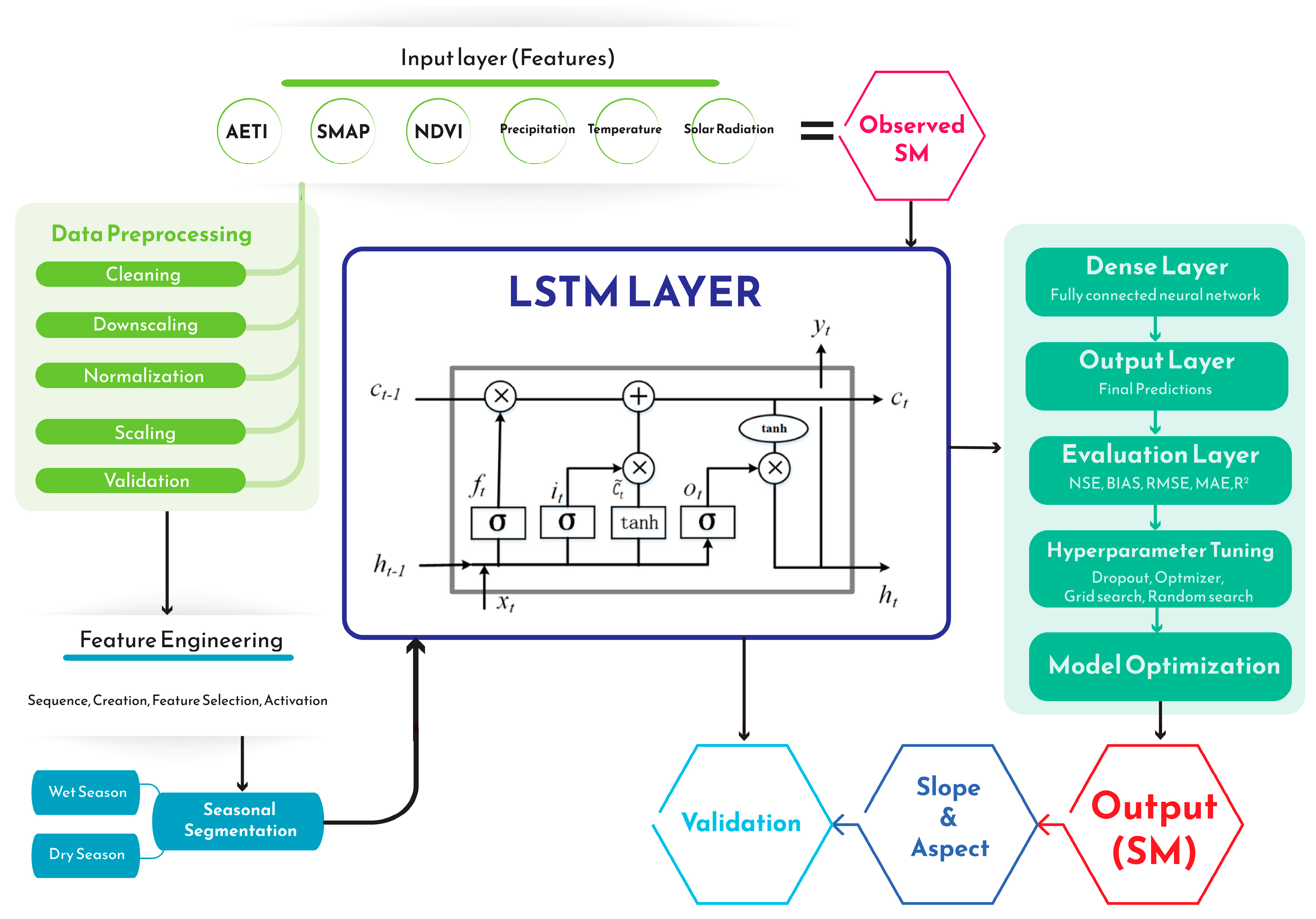
A schematic overview of the LSTM model workflow, including data preprocessing, feature engineering, model architecture, and evaluation steps, is shown in Figure 2.

2.3.3. Model Application and Evaluation

The trained LSTM model was applied over the period 10 December 2019–31 July 2024, across 222 agricultural sites in the study area. Among these sites, 100 contained stone bunds, whereas 122 did not. The model was used to generate daily soil moisture predictions at each site. These predictions were then analyzed both temporally and spatially to evaluate patterns in moisture variability and to assess the influence of conservation structures. The temporal evaluation involved comparing the predicted and observed soil moisture time series at sites with and without stone bunds. Spatial analysis was conducted using aggregated seasonal and annual soil moisture predictions across the 222 locations. To assess the statistical significance of moisture differences between stone-bunded and non-bunded fields, a paired t test was applied.

3. Results

3.1. Data Evaluation and Refinement

3.1.1. Dataset Selection and Downscaling

Among the three products, the SMAP 1 km dataset consistently outperformed the others (

Table 4. Comparison of daily in situ soil moisture with the obtained datasets (2019–2024).

Metrics	SMAP (1 km)	SMAP (9 km)	NASA Power
Correlation coefficient (r)	0.802	0.901	0.894
Coefficient of Determination (R2)	0.643	0.812	0.799
Nash–Sutcliffe Efficiency (NSE)	0.588	−4.396	−4.093
Root Mean Square Error (RMSE)	0.056	0.202	0.197
Mean Absolute Error (MAE)	0.036	0.121	0.116
Bias	0.002	0.12	0.115
Mean	0.127	0.245	0.24
Median	0.091	0.12	0.12
Standard Deviation (σ)	0.090	0.237	0.233

), resulting in the highest NSE (0.588), lowest RMSE (0.056), and minimal bias (0.002). SMAP 9 km and NASA POWER showed relatively high correlation coefficients (0.901 and 0.894, respectively) but performed poorly across other metrics, including NSE (−4.396 and −4.093).

All comparisons were based on 1912 daily paired observations between satellite or reanalysis products and in situ soil moisture measurements (2019–2024). The negative NSE values observed for SMAP 9 km and NASA POWER indicate that these datasets perform worse than a mean predictor. This poor performance likely results from their coarse spatial resolution and inability to capture localized soil–vegetation–atmosphere interactions that strongly influence field-scale soil moisture variability.

The RF-based temporal gap-filling method showed consistently high accuracy across the validation folds, with R² values of 0.99 for SMAP and 0.91 for the NDVI, confirming strong model robustness. The ET₀-based temporal disaggregation of AETI yielded an R² of 0.89. The corresponding RMSE values were (SMAP: 0.013; NDVI: 0.05; AETI: 0.20), confirming strong agreement between the downscaled outputs and reference data. Seasonal comparisons also revealed stable performance throughout the rainy season (June–September), with MAEs ranging from 0.034 to 0.042 and RMSE values ranging from 0.048 to 0.060. These findings affirm the reliability of the method across varying hydrological conditions, especially during peak vegetation and moisture periods.

3.1.2. Relationships Between Predictors and Observed Soil Moisture

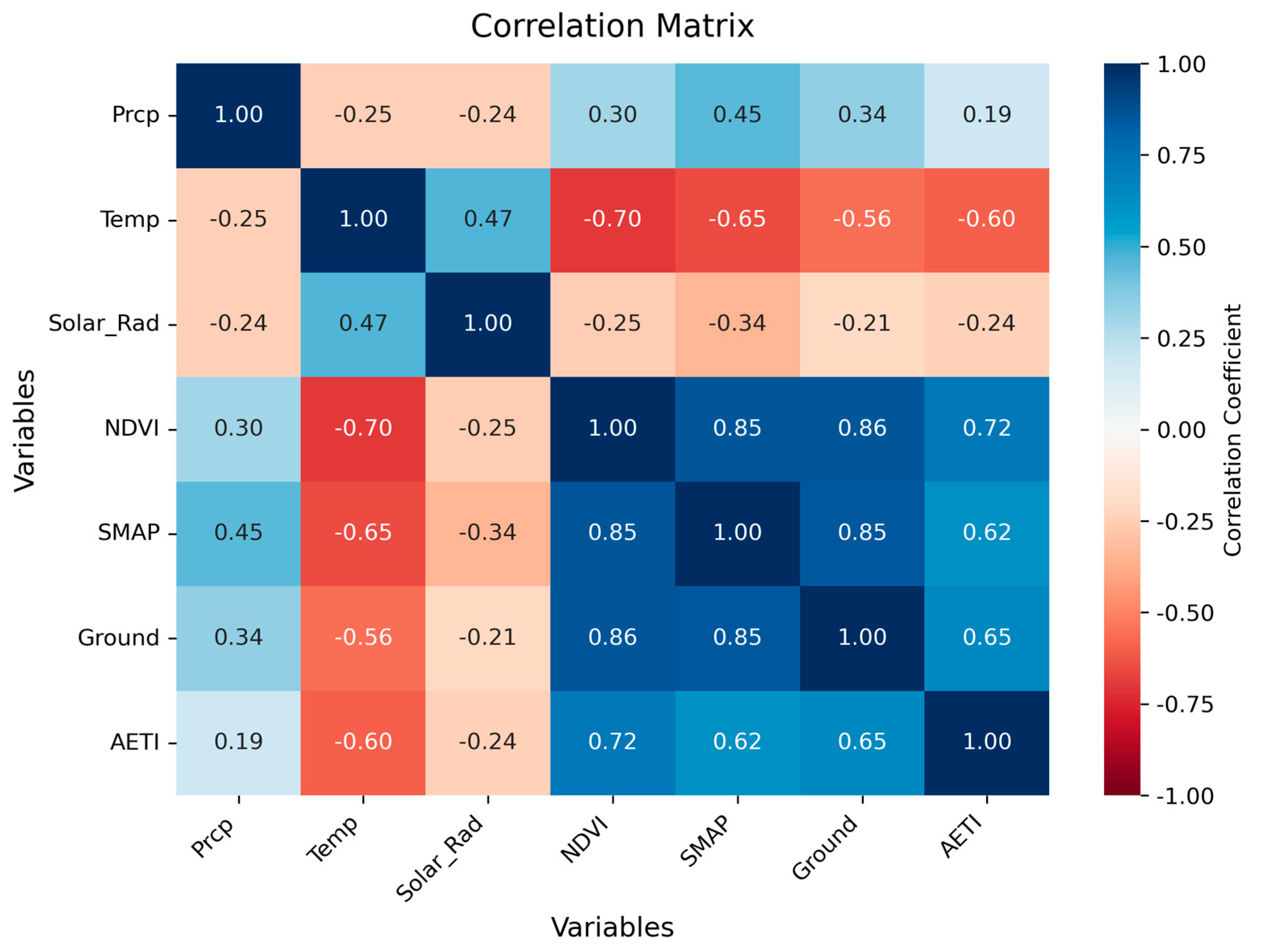
The strongest positive correlations with observed soil moisture corresponded to NDVI (r = 0.86), SMAP (r = 0.85), and AETI (r = 0.65) (Figure 3). These variables are considered central for the model’s ability to track vegetation conditions, antecedent soil moisture, and evapotranspiration dynamics. Precipitation (r = 0.34) showed a weaker yet expected positive correlation with soil moisture, reflecting the influence of rainfall events on short-term moisture variation. Conversely, temperature (r = −0.56) and solar radiation (r = −0.21) were negatively correlated with soil moisture, indicating their roles in driving evapotranspiration and soil drying. Despite their weaker direct correlations, temperature and solar radiation were retained in the model because of their indirect but important roles in moisture depletion. Although precipitation showed a weak daily correlation with observed soil moisture, it was retained as a predictor because it represents short-term recharge events that influence antecedent soil moisture conditions over multiple days.

3.2. Evaluation of the Soil Moisture Prediction Model

3.2.1. Model Performance Evaluation

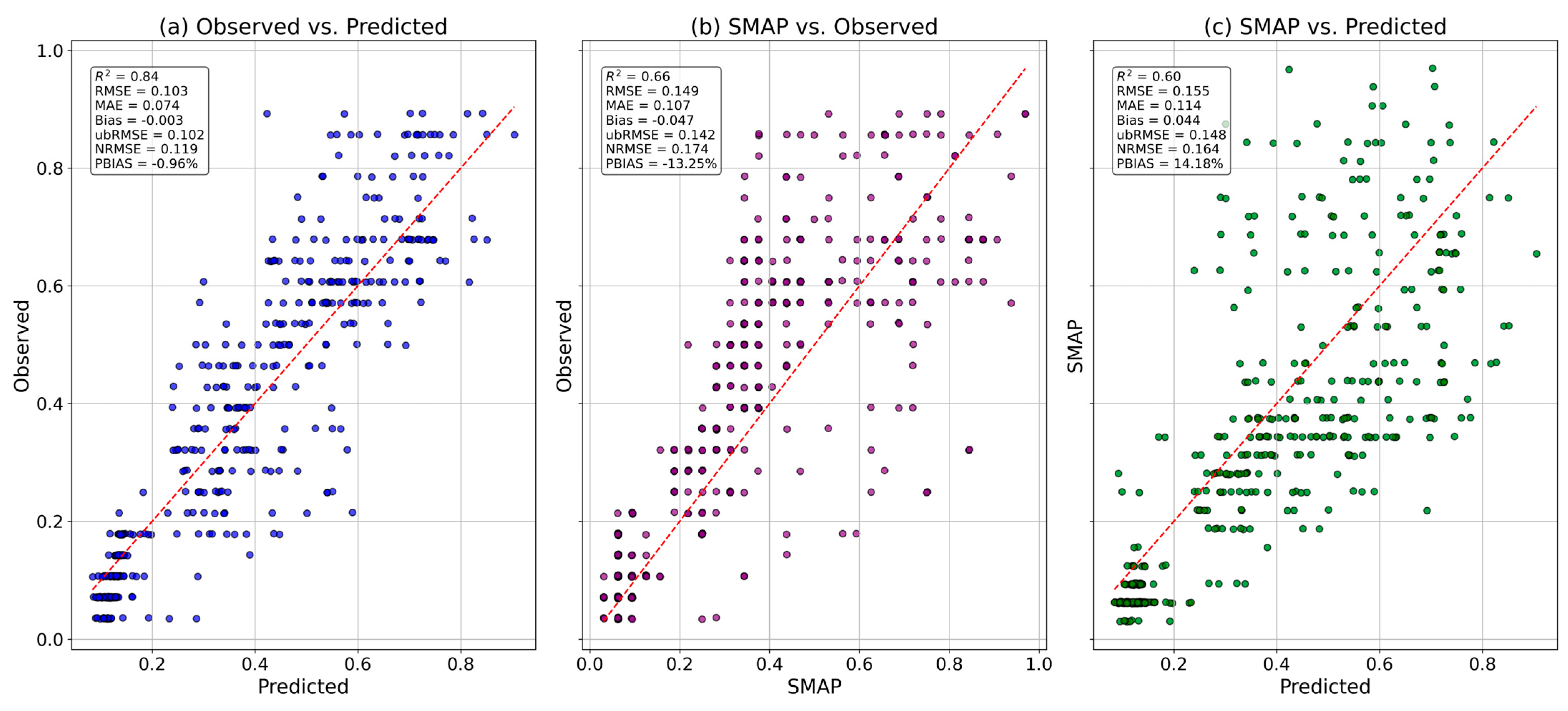
The LSTM model showed strong performance in predicting daily soil moisture across diverse seasonal conditions. Figure 4 presents a comparative evaluation of model performance from three perspectives: (a) observed versus LSTM-predicted values, (b) SMAP-derived versus observed values, and (c) SMAP-derived versus LSTM-predicted values. The LSTM model showed excellent agreement with in situ observations, achieving a high coefficient of determination (R² = 0.84), low RMSE (0.103), MAE (0.074), unbiased RMSE (ubRMSE = 0.102), and normalized RMSE (NRMSE) of 0.120. The model showed negligible bias (−0.003) and a near-zero percent bias (PBIAS = −0.97%), indicating minimal over- or underestimation.

In contrast, SMAP-derived soil moisture showed lower agreement with the observed data. The SMAP model produced an R² of 0.66, higher RMSE (0.149), MAE (0.107), ubRMSE (0.142), and NRMSE (0.174), along with a more pronounced negative bias (−0.047) and PBIAS of −13.24%, indicating a tendency to underestimate soil moisture. A direct comparison between LSTM and SMAP revealed that SMAP consistently overestimated values relative to LSTM-modeled soil moisture, particularly during wetter conditions. This was reflected in a positive bias of 0.044 and a PBIAS of 14.15%. Although the LSTM and SMAP predictions were moderately correlated (R² = 0.60), the LSTM model provided substantially better alignment with the observed values. Across all metrics, the LSTM model outperformed SMAP, achieving reductions of 30.9% in RMSE, 30.8% in MAE, 28.2% in ubRMSE, and 31.0% in NRMSE. The model also reduced the magnitude of bias by 93.6%. These results highlight the effectiveness of the model in capturing daily soil moisture variability and correcting systematic errors commonly found in satellite-derived estimates, especially in semiarid conditions where fine-scale resolution is critical.

Variable importance analysis revealed that the NDVI and AETI were the most influential features, contributing the greatest increases in MSE (0.0274 and 0.0286, respectively). SMAP also contributed to the model, although with a lower importance score (0.0023), likely because of its coarser native resolution and overlap with other features. The contributions of temperature, solar radiation, and precipitation were smaller but still meaningful, confirming their relevance in explaining temporal soil moisture dynamics under varying climatic conditions.

3.2.2. Spatiotemporal Evaluation of Model Performance

Compared with the SMAP product, the LSTM-modeled soil moisture showed better seasonal performance (

Table 5. Seasonal comparison of LSTM-modeled soil moisture with SMAP-derived soil moisture (Test Set).

Season	Model	R2	RMSE	MAE	ubRMSE	NRMSE	Bias	PBIAS
Dry	LSTM	0.76	0.05	0.04	0.05	0.09	0.02	13.66
Dry	SMAP	0.54	0.07	0.05	0.06	0.12	−0.03	−20.09
Wet	LSTM	0.58	0.13	0.10	0.13	0.17	−0.02	−3.80
Wet	SMAP	0.11	0.19	0.15	0.18	0.24	−0.06	−11.92

). During the dry season, the LSTM model resulted in an R² of 0.76, outperforming SMAP (0.54) by approximately 39%. RMSE and MAE were significantly reduced by 26.8% and 22.2%, respectively, whereas the ubRMSE and NRMSE also decreased by 25.9% and 26.8%, reflecting improved accuracy and reduced variance. Additionally, the LSTM model showed a positive PBIAS of 13.7%, indicating a slight overestimation aligned with seasonal recharge conditions, whereas SMAP exhibited a strong underestimation (PBIAS = −20.1%).

In the wet season, characterized by greater moisture variability, the LSTM-simulated soil moisture still outperformed SMAP, with an R² of 0.58, whereas SMAP (0.11) yielded a relative improvement of over 440%. The model reduced RMSE by 31.8%, MAE by 33.2%, and ubRMSE by 28.6%, demonstrating its ability to capture sharp transitions in moisture peaks. The LSTM also had a lower negative bias (−0.02 vs. −0.063) and a notably improved PBIAS (−3.8% vs. −11.9%). These seasonal insights further highlight the model’s ability to capture soil moisture dynamics across contrasting climatic regimes.

Monthly analysis revealed considerable variation in both model and SMAP performance across different hydrological periods. The LSTM model consistently outperformed SMAP during transitional months such as April, June, and October, where rapid soil moisture shifts typically occur. For example, in April, the LSTM model achieved a higher R² (0.798 vs. 0.654) and reduced the RMSE and MAE by 23.6% and 24.7%, respectively. Similarly, in June, the RMSE was reduced by 28.4%, indicating better alignment with in situ observations. In dry-season months such as November and December, where SMAP showed strong bias and an inflated NRMSE (up to 2.76), the LSTM model significantly improved accuracy (NRMSE < 0.68) and minimized bias. Additionally, in December, the LSTM model reduced the RMSE by 59% and PBIAS by 62% compared with those of SMAP, effectively capturing low-moisture conditions. The LSTM model outperformed SMAP in 9 out of 12 months across most key metrics (RMSE, MAE, and PBIAS), confirming its capacity to adapt to monthly scale variability and climatic transitions.

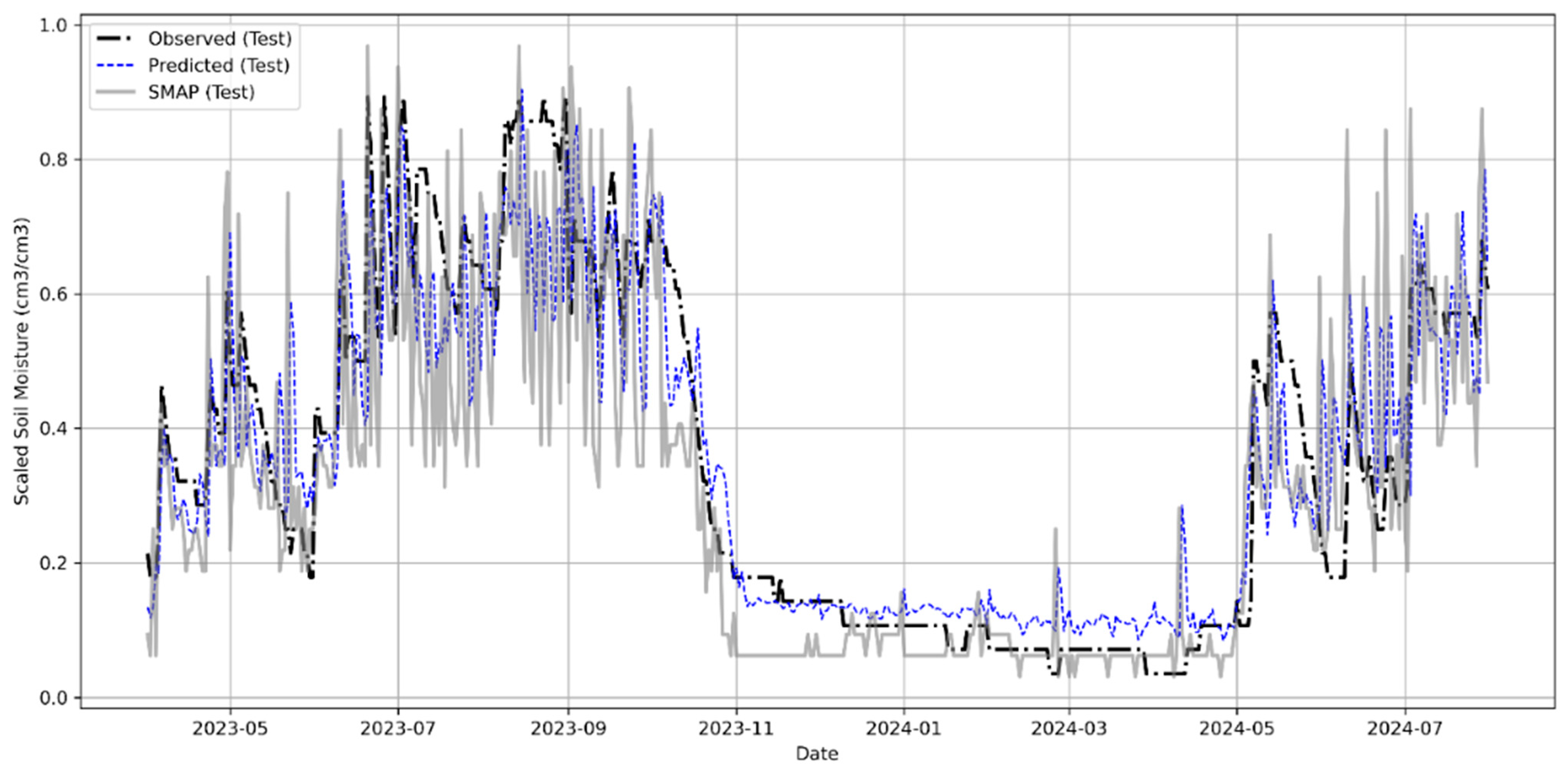
The temporal dynamics of observed, LSTM-predicted and SMAP-derived soil moisture data for the test period spanning from April 2023 to July 2024 are shown in Figure 5. The LSTM model closely follows observed ground measurements, capturing both seasonal transitions and short-term fluctuations. In contrast, the SMAP product exhibits a noticeable smoothing effect, often underestimating peak moisture levels during the wet season (e.g., June–July 2023) and failing to reflect abrupt drops during dry periods (e.g., December 2023–March 2024). The LSTM-modeled soil moisture thus captures both gradual and rapid hydrological shifts, addressing the concern of capturing fine-scale temporal dynamics more effectively than satellite-derived products do.

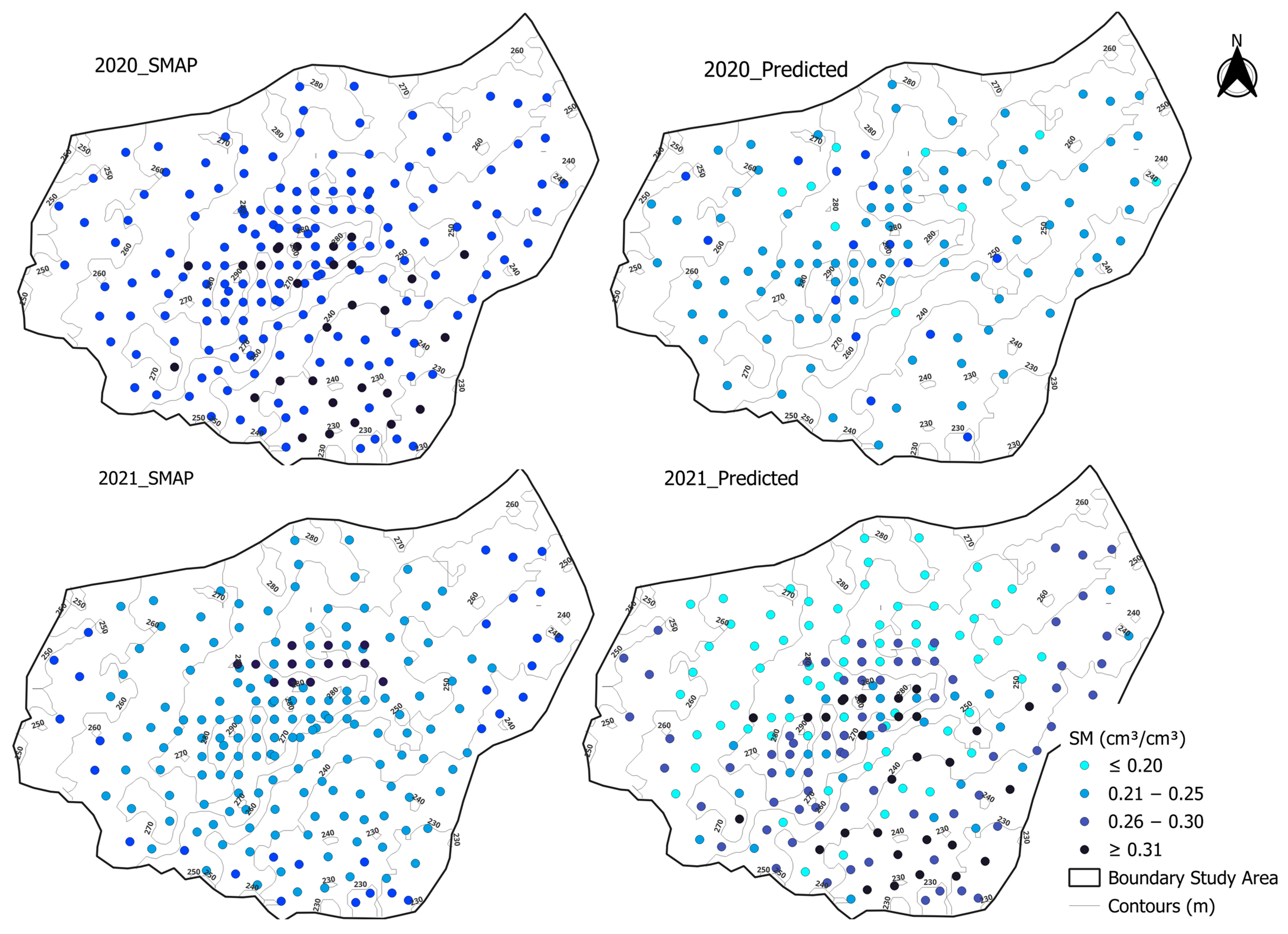
The spatial distributions of the soil moisture derived from both SMAP and the LSTM models from 2020 to 2023 are shown in Figure 6. The LSTM predictions clearly demonstrate a wider and more realistic spread of soil moisture values, ranging from ≤0.20 cm³/cm³ to ≥0.31 cm³/cm³, than SMAP, which predominantly clusters in the moderate range of 0.21–0.25 cm³/cm³. The LSTM model effectively captures higher soil moisture contents in elevated and central regions, which are typically influenced by terrain-induced runoff accumulation, revealing more fine-scale spatial variation than SMAP.

In 2020 and 2022, the LSTM model predicted 114% more high-moisture points (≥0.31 cm³/cm³) than SMAP, with an even greater increase observed in 2021 (167%) and 2023 (209%). This year-to-year variability reflects the influence of rainfall anomalies, as 2021 experienced above-average precipitation, whereas 2023 was characterized by a delayed onset of rain and reduced soil moisture persistence. This consistent pattern highlights the enhanced ability of the model to detect localized soil moisture enrichment, especially in years with pronounced hydrological contrasts. Additionally, at 65% to 85% of the spatial points, the LSTM-predicted values were higher than the SMAP values, confirming its robustness in estimating soil moisture under diverse climatic and topographic conditions. These results not only demonstrate the better spatial performance of LSTM-modeled soil moisture but also indirectly reflect the effectiveness of land management practices such as stone bunds in improving moisture retention across the landscape.

3.3. Model Performance in the Stone Bund and Control Areas

3.3.1. Temporal Assessment

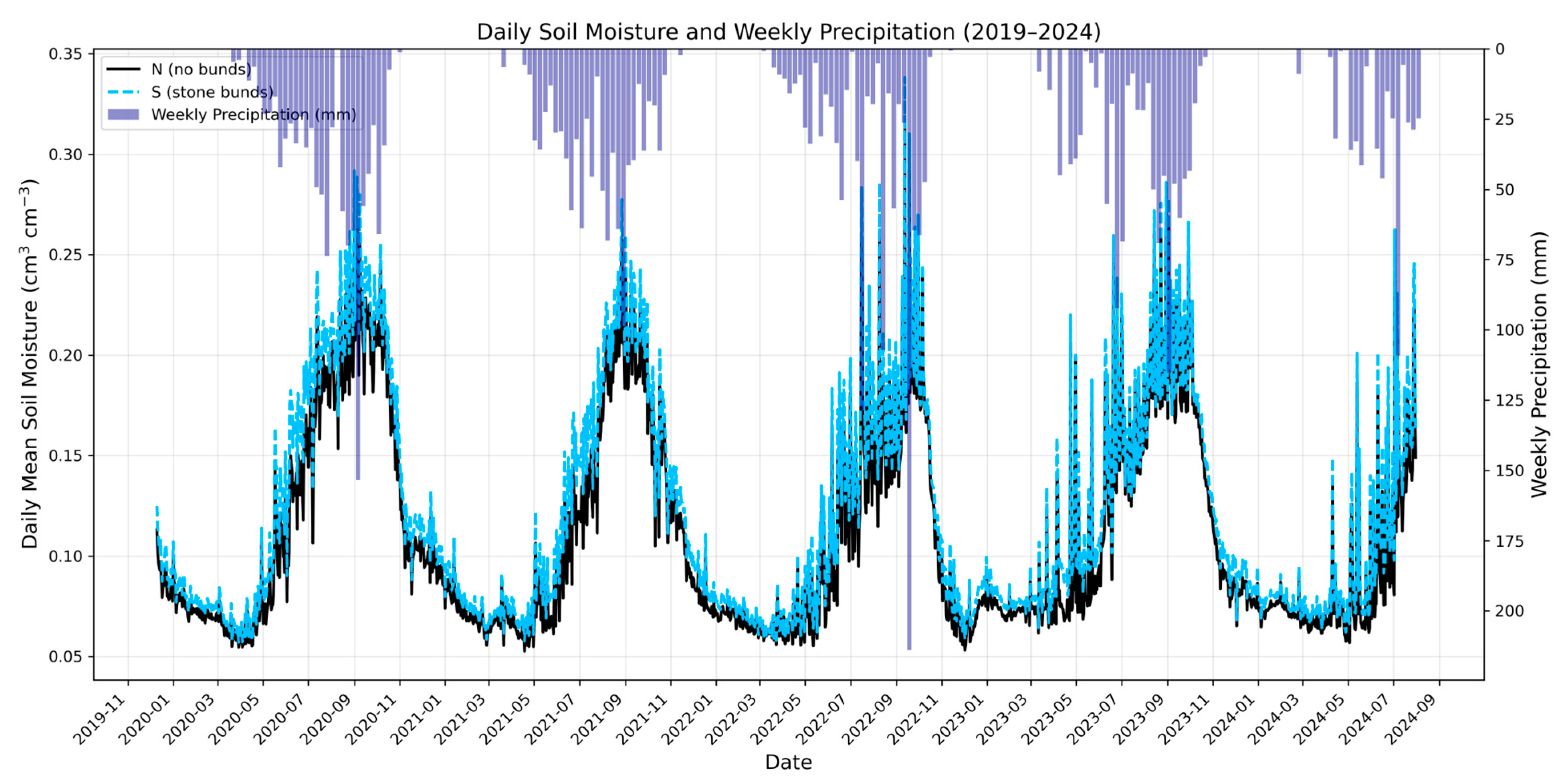
The aggregated daily average soil moisture dynamics from 2019 to 2024 across 222 monitoring sites with (S) and without (N) stone bunds, alongside precipitation patterns, are shown in Figure 7. Throughout this period, stone-bunded areas consistently maintained higher soil moisture levels compared to non-bunded sites. The difference was statistically significant across all years, with t statistics ranging from −2.367–−3.227 and corresponding p values consistently below 0.0026. In 2019, the average soil moisture at the stone-bunded sites was 0.197 cm³/cm³, compared to 0.188 cm³/cm³ in non-bunded areas (a 4.9% increase). This pattern persisted in subsequent years, with the annual average soil moisture at stone-bunded sites exceeding that of non-bunded areas by 4.1% to 6.0%, confirming the long-term hydrological benefit of stone bunds.

Seasonal analysis also showed that stone-bunded areas experienced a 5.3% improvement in soil moisture during the wet season and a 4.0% increase during the dry season, indicating enhanced infiltration during rainfall and prolonged retention during dry spells. Monthly comparisons further emphasized this effect, with an increase in soil moisture ranging from 2.9% to 13.8%. For example, in August 2020, stone-bunded sites averaged 0.318 cm³/cm³, while non-bunded areas measured 0.298 cm³/cm³, a 6.7% increase. Additionally, stone-bunded areas displayed a more gradual decline in soil moisture during dry spells, highlighting their effectiveness in reducing runoff and buffering against drought. The strong synchronization between rainfall events and soil moisture spikes, especially at the S site, confirms that stone bunds not only enhance short-term moisture retention but also support sustained water availability under increasing climatic variability.

3.3.2. Spatial Assessment

The spatial distribution of soil moisture from 2020 to 2023, which compares sites with (S) and without (N) stone bunds, is shown in Figure 8a,b. The dark blue symbols (≥0.31 cm³/cm³), indicative of elevated moisture levels, are consistently more prominent across stone-bunded sites every year, reflecting both temporal and spatial advantages of bund implementation. These patterns not only persist over time but are also widespread across different terrain zones, emphasizing the effectiveness of stone bunds in enhancing localized moisture retention. Quantitatively, stone-bunded sites presented 2 to 3 times more high-moisture locations than non-bunded areas. For example, in 2022, the number of high-soil moisture sites was 165% greater in stone-bunded regions, increasing to over 210% in 2023. These trends align with annual averages, with stone-bunded sites showing 7.55% to 11.28% higher mean soil moisture, 5.43% to 10.66% greater maximum values, and 4.35% to 9.68% higher minimum values compared to non-bunded areas. These findings confirm that stone bunds not only improve year-round moisture availability but also enhance spatial resilience across diverse microenvironments, making them critical nature-based solutions in dryland agriculture.

3.3.3. Topographic Controls on Predicted Soil Moisture

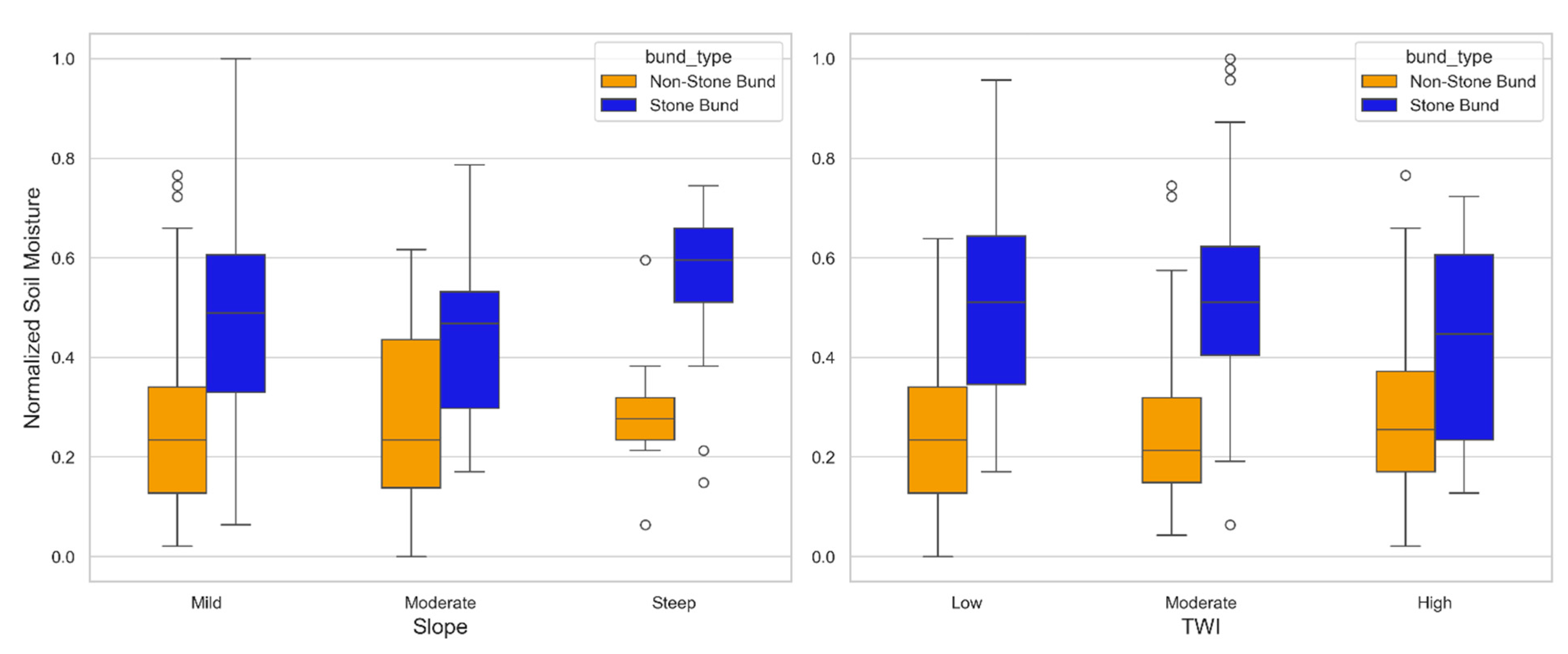
The normalized soil moisture data for stone bund and non-stone bund sites across different slopes and TWI categories are shown in Figure 9. In the Mild and Steep slope categories, stone bund areas consistently have greater moisture retention, suggesting that bunds effectively capture and hold water across different types of terrain. In the TWI comparison, stone bunds retain more moisture across all TWI categories, with the most pronounced effect observed in areas with low and moderate TWIs. The mild slope category revealed a highly significant difference between stone-bunded and non-bunded sites (p value = 0), while the moderate slope category showed a moderately significant difference (p value = 0.033), and the steep slope category displayed an extremely significant difference (p value = 0). Similarly, the TWI comparison indicated substantial differences, with low TWI sites having the most significant difference (p value = 0), followed by moderate TWI sites (p value = 0). These findings highlight the role of stone bunds in enhancing moisture retention, particularly in locations with favorable topographic characteristics such as moderate TWIs. The results further highlight the potential of stone bunds to improve soil moisture stability in a range of landscapes, contributing to effective soil and water conservation.

4. Discussion

4.1. Data Integration and Preprocessing

This study presents a comprehensive and scalable approach for high-resolution soil moisture prediction and the assessment of nature-based soil and water conservation practices in semiarid, fragmented landscapes. By integrating remote sensing data, in situ observations, and machine learning techniques, specifically Random Forest and LSTM networks, the proposed workflow provides practical insight into field-scale soil–water dynamics and addresses critical gaps in both soil moisture modeling and conservation impact evaluation.

The integration of multisource satellite data in this study required addressing inherent mismatches in spatiotemporal variability, which is a common limitation in remote sensing applications for smallholder agriculture [32,33,55,56,57]. The choice of gap-filling methods was driven by the nature of limitations within each dataset: sporadic missing values in SMAP and NDVI versus systematic temporal aggregation in AETI. While Random Forest has been widely applied for spatial downscaling of coarse resolution products, its application here for temporal gap-filling leverages its capacity to learn complex relationships between moisture-related variables and meteorological drivers. ET₀-based disaggregation of decadal AETI assumes a proportional distribution of evapotranspiration within decadal periods and relies on a well-established relationship between actual and reference ETs. These preprocessing decisions represent trade-offs between model complexity, data availability and computational feasibility, highlighting ongoing challenges in harmonizing satellite products for field-scale hydrological monitoring in data-sparse regions. The consistency of gap-filled estimates during the rainy season is particularly relevant given that soil moisture variability during this period is critical for decision-making [58].

4.2. Model Performance and Predictors

Integration of multiple predictors, including AETI, NDVI, temperature, precipitation, and solar radiation, enhances the ability of the model to capture the complex interactions influencing soil moisture dynamics. Among these, remotely sensed AETI plays a vital role in soil moisture estimation by reflecting evapotranspiration, directly linking soil moisture with vegetation and atmospheric conditions [59]. This is particularly important in semiarid agricultural regions, where evapotranspiration is a critical component of the water cycle. Similarly, NDVI, which represents vegetation health and cover, provides insights into moisture uptake and has a strong correlation with soil moisture variability. The sensitivity of the model to AETI and NDVI highlights their role as primary drivers of soil moisture dynamics. The inclusion of T, P, and Rs further refines the model by accounting for additional hydrological processes that influence soil moisture variability, such as precipitation events and solar-induced evaporation. These findings align with recent research that underscores the importance of integrating multisource predictors with high-resolution in situ observations to achieve robust and reliable soil moisture estimations.

The LSTM model trained on in situ datasets showed strong predictive performance across both dry and wet seasons. It achieved higher accuracy than SMAP in all key evaluation metrics, including a 30–59% reduction in RMSE and a 93% reduction in prediction bias. These results affirm the model’s ability to capture both short-term variability (e.g., daily rainfall pulses and rapid drying) and long-term seasonal dynamics. This is particularly important in semiarid climates such as northern Ghana, where rainfall is erratic and where soil moisture storage is essential for agricultural resilience. The evaluation metrics used to assess the soil moisture prediction model, such as RMSE, R², MAE, NSE, and bias, offer a comprehensive view of its performance. Low RMSE and MAE values indicate the model’s effectiveness in minimizing prediction errors, while high R² and positive NSE values highlight its success in capturing the observed soil moisture variability and trends. These findings are consistent with research emphasizing the importance of using multiple metrics to assess model performance fully, as each metric offers insights into different aspects of accuracy and reliability [39,60,61]. The near-zero bias value suggests that the model minimizes systematic errors, confirming its reliability for practical soil moisture applications. The obtained R² (0.84) compares reasonably with previous soil-moisture modeling studies. The study by [62] reported R² = 0.78 using an LSTM–GRU hybrid model in semiarid India, and [63] achieved R² = 0.81 in Mediterranean croplands demonstrating competitive or superior performance of the present framework. The model also outperforms SMAP data, particularly in terms of error reduction and stronger correlations with observed values, highlighting the potential of combining high-resolution environmental datasets with ML for more accurate soil moisture estimation. These capabilities and improvement in model representation have also been suggested by other studies [36,64]. Future work could include ensemble LSTM runs or bootstrap resampling to estimate confidence intervals for the RMSE improvements and trade-offs and assess uncertainty in model predictions. Additionally, by integrating the broad spatial coverage of satellite data with the localized accuracy of in situ measurements, the model provides high-resolution soil moisture estimates, a significant advancement in soil moisture monitoring. This integration is crucial for overcoming the limitations of satellite data, which often struggle to capture fine-scale heterogeneity, and to overcome the challenge of obtaining sparse in situ data for large-scale applications.

4.3. Stone-Bund Impact and Implications

When scaling to larger spatial areas, the ability of the model to capture soil moisture variability was validated through its strong performance relative to the 1 km SMAP dataset. By incorporating higher-resolution predictors, the model not only improved accuracy but also revealed spatial patterns of soil moisture across broader regions. This capability is particularly significant for assessing land management practices, such as stone bunds, in conserving soil moisture across diverse landscapes. The effectiveness of stone bunds in improving soil moisture retention has been widely studied, particularly through in situ monitoring, where small-scale observations demonstrate their potential for enhancing water retention on steep slopes [24,27,65,66]. However, most studies have focused on these localized settings, and their applicability to larger-scale areas remains limited. In this study, the LSTM framework provides spatially explicit evidence that stone-bunded sites maintained 4–6% higher soil moisture on average than non-bunded fields, confirming their hydrological benefit under variable topographic conditions. The ability of the model to accurately detect and quantify the impact of stone bunds enhances its application, especially when addressing diverse topographies and scales. This modeling approach offers a more precise and spatially comprehensive assessment of stone bund effectiveness, providing insights for sustainable land management and soil conservation practices.

The effectiveness of stone bunds in improving soil moisture retention varied across different topographic conditions, with the greatest improvement observed in areas with steep slopes and low to moderate TWI values. In areas with steeper slopes, stone bunds significantly enhanced soil moisture retention, as these regions typically face greater runoff, and water retention capabilities of the bunds were particularly beneficial under these conditions. In moderate slopes and high TWI regions, the presence of stone bunds showed a relatively moderate improvement, reflecting the fact that the effectiveness of the bunds was slightly less pronounced, although still notable. These findings highlight the need for targeted land management strategies in which the design and placement of stone bunds are optimized for varying slope gradients [67,68].

In the context of capturing spatial patterns, sensitivity of the model to spatial variation proved particularly valuable in fragmented landscapes, such as smallholder farms, where land use and management are highly heterogeneous. By integrating diverse datasets and leveraging ML, the approach provides high-resolution estimates even in areas lacking dense ground monitoring. In future research, further integration of higher-resolution datasets and expansion of the model’s application across different regions and climate regimes can improve the accuracy and scalability of soil moisture predictions. This research provides a foundation for effective soil moisture monitoring and sustainable management of agricultural water resources, providing a comprehensive, data-driven framework for the ongoing monitoring of land conservation practices and the assessment of their effectiveness across semiarid landscapes.

These findings have direct policy relevance for The Savannah Zone Agricultural Productivity Improvement Project (SAPIP) in Ghana and FAO climate-adaptation programs, which promote sustainable land and water management. The spatially explicit model outputs can guide priority zones for bund installation, soil–water conservation, and drought-resilience interventions.

This study has several limitations: (1) it focuses on a single agroecological zone (Upper West Region, Ghana), which may limit generalization across climates; (2) the five-year temporal span restricts long-term trend analysis; (3) potential overfitting remains possible owing to limited ground-measurement sites; and (4) uncertainty in gap-filled data could propagate into model outputs. Future work should expand to multiyear and multisite analyses, integrate ensemble LSTM runs to quantify uncertainty, and combine additional data sources such as GNSS-R, SAR, or UAV LiDAR for improved soil-moisture retrieval across African drylands.

5. Conclusions

This study demonstrates the effectiveness of integrating high-resolution remote sensing data, in situ measurements, and machine learning approaches for soil moisture prediction and evaluating conservation practices in semiarid, fragmented landscapes. The combination of Random Forest for gap-filling and LSTM networks for temporal prediction provides a reliable framework for capturing fine-scale spatial and temporal soil-moisture variability. By employing this integrated modeling framework, this study successfully quantified the impact of stone bunds on soil moisture retention in semiarid zones of West Africa.

The results confirm that the LSTM model achieves high predictive accuracy (R² = 0.84) and effectively corrects satellite biases while detecting measurable improvements in soil moisture within stone-bunded areas. These findings highlight the hydrological value of nature-based soil- and water-conservation measures for improving drought resilience and sustaining agricultural productivity in data-scarce drylands.

Future work could integrate advanced observation sources such as GNSS-R, SAR, and UAV-LiDAR data to refine soil-moisture estimation and test model transferability across multiple African dryland regions. This will strengthen large-scale monitoring and support climate-resilient land management under diverse environmental conditions.

References

1. McColl, K.A.; Alemohammad, S.H.; Akbar, R.; Konings, A.G.; Yueh, S.; Entekhabi, D. The Global Distribution and Dynamics of Surface Soil Moisture. Nat. Geosci. 2017, 10, 100–104. [Google Scholar] [CrossRef]
2. Dobriyal, P.; Qureshi, A.; Badola, R.; Hussain, S.A. A Review of the Methods Available for Estimating Soil Moisture and Its Implications for Water Resource Management. J. Hydrol. 2012, 458–459, 110–117. [Google Scholar] [CrossRef]
3. Schubert, S.; Dole, R.; vandenDool, H.; Suarez, M.; Waliser, D. Prospects for Improved Forecasts of Weather and Short-Term Climate Variability on Subseasonal (2-Week to 2-Month) Times Scales; NASA: Washington, DC, USA, 2002. [Google Scholar]
4. Bolten, J.D.; Crow, W.T.; Zhan, X.; Jackson, T.J.; Reynolds, C.A. Evaluating the Utility of Remotely Sensed Soil Moisture Retrievals for Operational Agricultural Drought Monitoring. IEEE J. Sel. Top. Appl. Earth Obs. Remote Sens. 2009, 3, 57–66. [Google Scholar] [CrossRef]
5. Sheffield, J.; Goteti, G.; Wen, F.; Wood, E.F. A Simulated Soil Moisture Based Drought Analysis for the United States. J. Geophys. Res. Atmos. 2004, 109, D24108. [Google Scholar] [CrossRef]
6. Western, A.W.; Grayson, R.B.; Blöschl, G. Scaling of Soil Moisture: A Hydrologic Perspective. Annu. Rev. Earth Planet. Sci. 2002, 30, 149–180. [Google Scholar] [CrossRef]
7. Kannenberg, S.A.; Anderegg, W.R.; Barnes, M.L.; Dannenberg, M.P.; Knapp, A.K. Dominant Role of Soil Moisture in Mediating Carbon and Water Fluxes in Dryland Ecosystems. Nat. Geosci. 2024, 17, 38–43. [Google Scholar] [CrossRef]
8. Robinson, D.A.; Campbell, C.S.; Hopmans, J.W.; Hornbuckle, B.K.; Jones, S.B.; Knight, R.; Ogden, F.; Selker, J.; Wendroth, O. Soil Moisture Measurement for Ecological and Hydrological Watershed-scale Observatories: A Review. Vadose Zone J. 2008, 7, 358–389. [Google Scholar] [CrossRef]
9. Loucks, D.P.; Van Beek, E. Water Resources Planning and Management: An Overview. In Water Resource Systems Planning and Management; Springer International Publishing: Cham, Switzerland, 2017; pp. 1–49. ISBN 978-3-319-44232-7. [Google Scholar]
10. Sinore, T.; Wang, F. Impact of Climate Change on Agriculture and Adaptation Strategies in Ethiopia: A Meta-Analysis. Heliyon 2024, 10, e26103. [Google Scholar] [CrossRef]
11. Togneri, R.; Felipe dos Santos, D.; Camponogara, G.; Nagano, H.; Custódio, G.; Prati, R.; Fernandes, S.; Kamienski, C. Soil Moisture Forecast for Smart Irrigation: The Primetime for Machine Learning. Expert Syst. Appl. 2022, 207, 117653. [Google Scholar] [CrossRef]
12. Ritchie, H. Increasing Agricultural Productivity Across Sub-Saharan Africa Is One of the Most Important Problems This Century; WorldInData.org; MedBox: Laguna Hills, CA, USA, 2022. [Google Scholar]
13. Tefera, M.L.; Giovanna Seddaiu; Alberto Carletti; Awada, H. Rainfall Variability and Drought in West Africa: Challenges and Implications for Rainfed Agriculture. Theor. Appl. Climatol. 2024, 156, 41. [Google Scholar] [CrossRef]
14. Sungmin, O.; Orth, R. Global Soil Moisture Data Derived through Machine Learning Trained with In-Situ Measurements. Sci. Data 2021, 8, 170. [Google Scholar] [CrossRef]
15. Moran, M.S.; Peters-Lidard, C.D.; Watts, J.M.; McElroy, S. Estimating Soil Moisture at the Watershed Scale with Satellite-Based Radar and Land Surface Models. Can. J. Remote Sens. 2004, 30, 805–826. [Google Scholar] [CrossRef]
16. Romano, N. Soil Moisture at Local Scale: Measurements and Simulations. J. Hydrol. 2014, 516, 6–20. [Google Scholar] [CrossRef]
17. Batjes, N.H. Harmonized Soil Property Values for Broad-Scale Modelling (WISE30sec) with Estimates of Global Soil Carbon Stocks. Geoderma 2016, 269, 61–68. [Google Scholar] [CrossRef]
18. Vergopolan, N.; Chaney, N.W.; Pan, M.; Sheffield, J.; Beck, H.E.; Ferguson, C.R.; Torres-Rojas, L.; Sadri, S.; Wood, E.F. SMAP-HydroBlocks, a 30-m Satellite-Based Soil Moisture Dataset for the Conterminous US. Sci. Data 2021, 8, 264. [Google Scholar] [CrossRef]
19. Peng, J.; Albergel, C.; Balenzano, A.; Brocca, L.; Cartus, O.; Cosh, M.H.; Crow, W.T.; Dabrowska-Zielinska, K.; Dadson, S.; Davidson, M.W.J.; et al. A Roadmap for High-Resolution Satellite Soil Moisture Applications—Confronting Product Characteristics with User Requirements. Remote Sens. Environ. 2021, 252, 112162. [Google Scholar] [CrossRef]
20. Skulovich, O.; Gentine, P. A Long-Term Consistent Artificial Intelligence and Remote Sensing-Based Soil Moisture Dataset. Sci. Data 2023, 10, 154. [Google Scholar] [CrossRef]
21. Vadez, V.; Grondin, A.; Chenu, K.; Henry, A.; Laplaze, L.; Millet, E.J.; Carminati, A. Crop Traits and Production under Drought. Nat. Rev. Earth Environ. 2024, 5, 211–225. [Google Scholar] [CrossRef]
22. Naazie, G.K.; Dakyaga, F.; Derbile, E.K. Agro-Ecological Intensification for Climate Change Adaptation: Tales on Soil and Water Management Practices of Smallholder Farmers in Rural Ghana. Discov. Sustain. 2023, 4, 27. [Google Scholar] [CrossRef]
23. Singh, R. Bunds. In Soil and Water Conservation Structures Design; Water Science and Technology Library; Springer Nature: Singapore, 2023; Volume 123, pp. 95–119. ISBN 978-981-19-8664-2. [Google Scholar]
24. Tefera, M.L.; Awada, H.; Pirastru, M.; Kombiok, J.M.; Adjebeng-Danquah, J.; Adombilla, R.; Asungre, P.A.; Mahama, G.; Carletti, A.; Seddaiu, G. Remote Sensing and Field Data Analysis to Evaluate the Impact of Stone Bunds on Rainfed Agriculture in West Africa. Land 2024, 13, 1654. [Google Scholar] [CrossRef]
25. Alemayehu, M.; Yohannes, F.; Dubale, P. Effect of Indigenous Stone Bunding (Kab) on Crop Yield at Mesobit-Gedeba, North Shoa, Ethiopia. Land Degrad. Dev. 2006, 17, 45–54. [Google Scholar] [CrossRef]
26. Meresa, M.; Tadesse, M.; Zeray, N. Effect of Soil and Water Conservation Structures on Smallholder Farmers’ Livelihood: Wenago District, Southern Ethiopia. Cogent Soc. Sci. 2023, 9, 2272305. [Google Scholar] [CrossRef]
27. Nyssen, J.; Poesen, J.; Gebremichael, D.; Vancampenhout, K.; D’aes, M.; Yihdego, G.; Govers, G.; Leirs, H.; Moeyersons, J.; Naudts, J. Interdisciplinary On-Site Evaluation of Stone Bunds to Control Soil Erosion on Cropland in Northern Ethiopia. Soil Tillage Res. 2007, 94, 151–163. [Google Scholar] [CrossRef]
28. Huang, L.; Pan, A.; Chen, F.; Guo, F.; Li, H.; Liu, L. A Novel Global Grid Model for Soil Moisture Retrieval Considering Geographical Disparity in Spaceborne GNSS-R. Satell. Navig. 2024, 5, 29. [Google Scholar] [CrossRef]
29. Tefera, M.L.; Seddaiu, G.; Carletti, A. Traditional In Situ Water Harvesting Practices and Agricultural Sustainability in Sub-Saharan Africa—A Meta-Analysis. Sustainability 2024, 16, 6427. [Google Scholar] [CrossRef]
30. Tavakol, A.; McDonough, K.R.; Rahmani, V.; Hutchinson, S.L.; Hutchinson, J.M.S. The Soil Moisture Data Bank: The Ground-Based, Model-Based, and Satellite-Based Soil Moisture Data. Remote Sens. Appl. Soc. Environ. 2021, 24, 100649. [Google Scholar] [CrossRef]
31. Brocca, L.; Ciabatta, L.; Massari, C.; Camici, S.; Tarpanelli, A. Soil Moisture for Hydrological Applications: Open Questions and New Opportunities. Water 2017, 9, 140. [Google Scholar] [CrossRef]
32. Vergopolan, N.; Sheffield, J.; Chaney, N.W.; Pan, M.; Beck, H.E.; Ferguson, C.R.; Torres-Rojas, L.; Eigenbrod, F.; Crow, W.; Wood, E.F. High-resolution Soil Moisture Data Reveal Complex Multi-scale Spatial Variability across the United States. Geophys. Res. Lett. 2022, 49, e2022GL098586. [Google Scholar] [CrossRef]
33. Peng, J.; Loew, A.; Merlin, O.; Verhoest, N.E. A Review of Spatial Downscaling of Satellite Remotely Sensed Soil Moisture. Rev. Geophys. 2017, 55, 341–366. [Google Scholar] [CrossRef]
34. Hengl, T.; Mendes de Jesus, J.; Heuvelink, G.B.; Ruiperez Gonzalez, M.; Kilibarda, M.; Blagotić, A.; Shangguan, W.; Wright, M.N.; Geng, X.; Bauer-Marschallinger, B. SoilGrids250m: Global Gridded Soil Information Based on Machine Learning. PLoS ONE 2017, 12, e0169748. [Google Scholar] [CrossRef]
35. Teshome, F.T.; Bayabil, H.K.; Schaffer, B.; Ampatzidis, Y.; Hoogenboom, G. Improving Soil Moisture Prediction with Deep Learning and Machine Learning Models. Comput. Electron. Agric. 2024, 226, 109414. [Google Scholar] [CrossRef]
36. Zhong, Y.; Hong, S.; Wei, Z.; Walker, J.P.; Wang, Y.; Huang, C. Spatial Downscaling of SMAP Soil Moisture Estimation Using Multiscale Geographically Weighted Regression during SMAPVEX16. J. Hydrol. 2024, 637, 131348. [Google Scholar] [CrossRef]
37. Hutengs, C.; Vohland, M. Downscaling Land Surface Temperatures at Regional Scales with Random Forest Regression. Remote Sens. Environ. 2016, 178, 127–141. [Google Scholar] [CrossRef]
38. Hochreiter, S.; Schmidhuber, J. Long Short-Term Memory. Neural Comput. 1997, 9, 1735–1780. [Google Scholar] [CrossRef] [PubMed]
39. Datta, P.; Faroughi, S.A. A Multihead LSTM Technique for Prognostic Prediction of Soil Moisture. Geoderma 2023, 433, 116452. [Google Scholar] [CrossRef]
40. Beven, K.J.; Kirkby, M.J. A Physically Based, Variable Contributing Area Model of Basin Hydrology/Un Modèle à Base Physique de Zone d’appel Variable de l’hydrologie Du Bassin Versant. Hydrol. Sci. J. 1979, 24, 43–69. [Google Scholar] [CrossRef]
41. O’Neill, P.E.C. SMAP Enhanced L3 Radiometer Global and Polar Grid Daily 9 Km EASE-Grid Soil Moisture, Version 6 (SPL3SMP_E); National Snow and Ice Data Center: Boulder, CO, USA, 2023. [Google Scholar] [CrossRef]
42. Lakshmi, V.; Fang, B. SMAP-Derived 1-Km Downscaled Surface Soil Moisture Product, Version 1; National Snow and Ice Data Center: Boulder, CO, USA, 2023. [Google Scholar] [CrossRef]
43. Luan, J.; Zhang, C.; Xu, B.; Xue, Y.; Ren, Y. The Predictive Performances of Random Forest Models with Limited Sample Size and Different Species Traits. Fish. Res. 2020, 227, 105534. [Google Scholar] [CrossRef]
44. Pang, B.; Yue, J.; Zhao, G.; Xu, Z. Statistical Downscaling of Temperature with the Random Forest Model. Adv. Meteorol. 2017, 2017, 1–11. [Google Scholar] [CrossRef]
45. Zhang, X.; Shen, H.; Huang, T.; Wu, Y.; Guo, B.; Liu, Z.; Luo, H.; Tang, J.; Zhou, H.; Wang, L.; et al. Improved Random Forest Algorithms for Increasing the Accuracy of Forest Aboveground Biomass Estimation Using Sentinel-2 Imagery. Ecol. Indic. 2024, 159, 111752. [Google Scholar] [CrossRef]
46. Danso, D.K.; Anquetin, S.; Diedhiou, A.; Lavaysse, C.; Kobea, A.; Touré, N.E. Spatio-temporal Variability of Cloud Cover Types in West Africa with Satellite-based and Reanalysis Data. Q. J. R. Meteorol. Soc. 2019, 145, 3715–3731. [Google Scholar] [CrossRef]
47. FAO. WaPOR Database Methodology: Level 1. Remote Sensing for Water Productivity Technical Report: Methodology Series; FAO: Rome, Italy, 2018; 72p. [Google Scholar]
48. Allen, R.G.; Pereira, L.S.; Raes, D.; Smith, M. Crop Evapotranspiration—Guidelines for Computing Crop Water Requirements (FAO Irrigation and Drainage Paper 56); Food and Agriculture Organization of the United Nations (FAO): Rome, Italy, 1998. [Google Scholar]
49. Sheth, V.; Tripathi, U.; Sharma, A. A Comparative Analysis of Machine Learning Algorithms for Classification Purpose. Procedia Comput. Sci. 2022, 215, 422–431. [Google Scholar] [CrossRef]
50. Yadav, D.K.; Kaushik, A.; Yadav, N. Predicting Machine Failures Using Machine Learning and Deep Learning Algorithms. Sustain. Manuf. Serv. Econ. 2024, 3, 100029. [Google Scholar] [CrossRef]
51. Pathak, S.; Quraishi, S.J.; Singh, A.; Singh, M.; Arora, K.; Ather, D. A Comparative Analysis of Machine Learning Models: SVM, Naïve Bayes, Random Forest, and LSTM in Predictive Analytics. In Proceedings of the 2023 3rd International Conference on Technological Advancements in Computational Sciences (ICTACS), Lahore, Pakistan, 20–22 February 2023; pp. 790–795. [Google Scholar] [CrossRef]
52. Li, Q.; Zhu, Y.; Shangguan, W.; Wang, X.; Li, L.; Yu, F. An Attention-Aware LSTM Model for Soil Moisture and Soil Temperature Prediction. Geoderma 2022, 409, 115651. [Google Scholar] [CrossRef]
53. Hefron, R.G.; Borghetti, B.J.; Christensen, J.C.; Kabban, C.M.S. Deep Long Short-Term Memory Structures Model Temporal Dependencies Improving Cognitive Workload Estimation. Pattern Recognit. Lett. 2017, 94, 96–104. [Google Scholar] [CrossRef]
54. Pedregosa, F.; Varoquaux, G.; Gramfort, A.; Michel, V.; Thirion, B.; Grisel, O.; Blondel, M.; Prettenhofer, P.; Weiss, R.; Dubourg, V.; et al. Scikit-Learn: Machine Learning in Python. J. Mach. Learn. Res. 2011, 12, 2825–2830. [Google Scholar]
55. Khaki, M.; Hendricks Franssen, H.-J.; Han, S.C. Multi-Mission Satellite Remote Sensing Data for Improving Land Hydrological Models via Data Assimilation. Sci. Rep. 2020, 10, 18791. [Google Scholar] [CrossRef]
56. Guan, Y.; Gu, X.; Slater, L.J.; Li, J.; Kong, D.; Zhang, X. Spatio-Temporal Variations in Global Surface Soil Moisture Based on Multiple Datasets: Intercomparison and Climate Drivers. J. Hydrol. 2023, 625, 130095. [Google Scholar] [CrossRef]
57. Tahmouresi, M.S.; Niksokhan, M.H.; Ehsani, A.H. Enhancing Spatial Resolution of Satellite Soil Moisture Data through Stacking Ensemble Learning Techniques. Sci. Rep. 2024, 14, 25454. [Google Scholar] [CrossRef]
58. Schneider, D.P.; Deser, C.; Fasullo, J.; Trenberth, K.E. Climate Data Guide Spurs Discovery and Understanding. Eos Trans. Am. Geophys. Union 2013, 94, 121–122. [Google Scholar] [CrossRef]
59. Awada, H.; Sirca, C.; Marras, S.; Castellini, M.; Spano, D.; Pirastru, M. Modelling Soil Moisture and Daily Actual Evapotranspiration: Integrating Remote Sensing Surface Energy Balance and 1D Richards Equation. Int. J. Appl. Earth Obs. Geoinform. 2024, 128, 103744. [Google Scholar] [CrossRef]
60. Willmott, C.J.; Robeson, S.M.; Matsuura, K. A Refined Index of Model Performance. Int. J. Climatol. 2012, 32, 2088–2094. [Google Scholar] [CrossRef]
61. Li, Q.; Li, Z.; Shangguan, W.; Wang, X.; Li, L.; Yu, F. Improving Soil Moisture Prediction Using a Novel Encoder-Decoder Model with Residual Learning. Comput. Electron. Agric. 2022, 195, 106816. [Google Scholar] [CrossRef]
62. Kandamali, D.F.; Porter, E.; Porter, W.M.; McLemore, A.; Kiobia, D.O.; Tavandashti, A.P.; Rains, G.C. Hybrid LSTM Method for Multistep Soil Moisture Prediction Using Historical Soil Moisture and Weather Data. AgriEngineering 2025, 7, 260. [Google Scholar] [CrossRef]
63. Graldi, G.; Zardi, D.; Vitti, A. Retrieving Soil Moisture at the Field Scale from Sentinel-1 Data over a Semi-Arid Mediterranean Agricultural Area. Remote Sens. 2023, 15, 2997. [Google Scholar] [CrossRef]
64. Karamouz, M.; Alipour, R.S.; Roohinia, M.; Fereshtehpour, M. A Remote Sensing Driven Soil Moisture Estimator: Uncertain Downscaling With Geostatistically Based Use of Ancillary Data. Water Resour. Res. 2022, 58, e2022WR031946. [Google Scholar] [CrossRef]
65. Klik, A.; Schürz, C.; Strohmeier, S.; Demelash Melaku, N.; Ziadat, F.; Schwen, A.; Zucca, C. Impact of Stone Bunds on Temporal and Spatial Variability of Soil Physical Properties: A Field Study from Northern Ethiopia. Land Degrad. Dev. 2018, 29, 585–595. [Google Scholar] [CrossRef]
66. Vancampenhout, K.; Nyssen, J.; Gebremichael, D.; Deckers, J.; Poesen, J.; Haile, M.; Moeyersons, J. Stone Bunds for Soil Conservation in the Northern Ethiopian Highlands: Impacts on Soil Fertility and Crop Yield. Soil Tillage Res. 2006, 90, 1–15. [Google Scholar] [CrossRef]
67. Masha, M.; Bojago, E.; Belayneh, M. Assessing the Impacts of Soil and Water Conservation Practices on Soil Physicochemical Properties in Contrasting Slope Landscapes of Southern Ethiopia. J. Agric. Food Res. 2023, 14, 100876. [Google Scholar] [CrossRef]
68. Bayisa, H.; Kebede, B.; Benti, F. Factors Influencing the Implementation and Adoption of Sustainable Land Management Practices on Wacaca Mountain in Central Highlands of Ethiopia. Environ. Model. Assess. 2025, 30, 53–70. [Google Scholar] [CrossRef]
Figure 1. Study area within Nandom District, Upper West Region, Ghana. The map shows the locations of fields with and without stone bunds. The Google Earth image shows one of the selected plots with stone bunds retrieved from earth.google.com.
Remotesensing 17 03651 g001
Figure 2. Overview of the soil moisture prediction model using an LSTM neural network. The diagram illustrates the data preprocessing, feature engineering, LSTM architecture, and model evaluation steps, integrating environmental variables for soil moisture estimation.
Remotesensing 17 03651 g002
Figure 3. Correlation matrix showing the relationships between meteorological and RS variables, including precipitation (P), temperature (T), solar radiation (Rs), downscaled NDVI, soil moisture (SMAP), and actual evapotranspiration (AETI), and the observed soil moisture (observed). The color scale represents the strength of the correlation, with red indicating negative correlations and blue indicating positive correlations.
Remotesensing 17 03651 g003
Figure 4. Comparison of predicted, SMAP, and observed soil moisture values with performance metrics from three perspectives: (a) observed versus LSTM-predicted values, (b) SMAP-derived versus observed values, and (c) SMAP-derived versus LSTM-predicted values. The dashed red line in all plots represents the 1:1 line.
Remotesensing 17 03651 g004
Figure 5. Daily temporal dynamics of observed, predicted, and SMAP-derived soil moisture over the test period (February 2023–July 2024).
Remotesensing 17 03651 g005
Figure 6. Spatial distributions of the predicted soil moisture and SMAP satellite-derived soil moisture from 2020–2023.
Remotesensing 17 03651 g006aRemotesensing 17 03651 g006b
Figure 7. Daily average soil moisture dynamics and precipitation patterns: Comparison between sites with (S) and without (N) Stone Bunds.
Remotesensing 17 03651 g007
Figure 8. Spatial annual soil moisture at sites with (a) and without (b) stone bunds (2020–2023).
Remotesensing 17 03651 g008
Figure 9. Relationships between the predicted soil moisture and topographic variables (slope and TWI) for stone bund and non-bunded sites.
Remotesensing 17 03651 g009