Deep Learning-Based Short- and Mid-Term Surface and Subsurface Soil Moisture Projections from Remote Sensing and Digital Soil Maps

Abstract

Accurate real-time information about soil moisture (SM) at a large scale is essential for improving hydrological modeling, managing water resources, and monitoring extreme weather events. This study presents a framework using convolutional long short-term memory (ConvLSTM) network to produce short- (1, 3, and 7 days ahead) and mid-term (14 and 30 days ahead) forecasts of SM at surface (0–10 cm) and subsurface (10–40 and 40–100 cm) soil layers across the contiguous U.S. The model was trained with five-year period (2018–2022) datasets including Soil Moisture Active Passive (SMAP) level 3 ancillary covariables, North American Land Data Assimilation System phase 2 (NLDAS-2) SM product, shortwave infrared reflectance from Moderate Resolution Imaging Spectroradiometer (MODIS), and terrain features (e.g., elevation, slope, curvature), as well as soil texture and bulk density maps from the Soil Landscape of the United States (SOLUS100) database. To develop and evaluate the model, the dataset was divided into three subsets: training (January 2018–January 2021), validation (2021), and testing (2022). The outputs were validated with observed in situ data from the Soil Climate Analysis Network (SCAN) and the United States Climate Reference Network (USCRN) soil moisture networks. The results indicated that the accuracy of SM forecasts decreased with increasing lead time, particularly in the surface (0–10 cm) and subsurface (10–40 cm) layers, where strong fluctuations driven by rainfall variability and evapotranspiration fluxes introduced greater uncertainty. Across all soil layers and lead times, the model achieved a median unbiased root mean square error (ubRMSE) of 0.04 cm³ cm⁻³ with a Pearson correlation coefficient of 0.61. Further, the performance of the model was evaluated with respect to both land cover and soil texture databases. Forecast accuracy was highest in coarse-textured soils, followed by medium- and fine-textured soils, likely because the greater penetration depth of microwave observations improves SM retrieval in sandy soils. Among land cover types, performance was strongest in grasslands and savannas and weakest in dense forests and shrublands, where dense vegetation attenuates the microwave signal and reduces SM estimation accuracy. These results demonstrate that the ConvLSTM framework provides skillful short- and mid-term forecasts of surface and subsurface soil moisture, offering valuable support for large-scale drought and flood monitoring.

1. Introduction

Soil moisture (SM) plays a critical role in monitoring the terrestrial water and energy cycles [1,2]. Accurate and timely SM information is essential for a wide range of applications at local to global scales, including weather forecasting [3], early warning systems for droughts and floods [4,5], landslide prediction [6], and wildfire risk assessment [7]. SM regulates key land surface fluxes such as evaporation, infiltration, runoff, and groundwater recharge. In particular, root zone SM (typically within the top 0–100 cm) is critical for coupling these surface and subsurface processes, which makes it a key variable for hydrological modeling and water resources management [1]. Despite its importance, accurate nowcasts (short-term forecast) and forecasts (mid- and long-term forecast) of surface and subsurface SM at regional to continental scales remain a challenge, mainly due to the limitations of current measurement and monitoring techniques.

While in situ monitoring networks provide high-quality multi-depth SM data, they are spatially sparse and only represent point-scale observations [8], which limits their application for large-scale monitoring. To overcome these limitations, satellite-based remote sensing (RS) has become a widely used method for monitoring SM. Among different RS techniques, L-band microwave observations (1–2 GHz) have shown strong sensitivity to soil dielectric properties and the ability to penetrate moderate vegetation cover, which makes them suitable for large-scale SM estimation [9]. The Soil Moisture Active and Passive (SMAP) mission, launched by NASA in 2015, is currently a prime example for satellite-based SM monitoring, which provides surface SM (0–5 cm) at spatial resolutions of 9 and 36 km (Level 3 product, L3) with revisit times of 2–3 days and root zone SM (0–100 cm) through data assimilation (level 4 product, L4) at 9 km resolution and 3 h intervals [10,11,12].

Although SMAP SM products represent a significant advancement, they include several limitations. As pointed out, the L3 product is limited to surface SM and does not capture subsurface conditions. The L4 product addresses this by assimilating brightness temperature data into a land surface model to estimate root zone SM. However, it provides only a depth-averaged SM value for the 0–100 cm soil profile. This averaging does not capture SM variability within the soil profile caused by processes such as surface evaporation, root water uptake, and deep percolation. Moreover, L3 and L4 products are limited by a data latency of about 2 days before public release, which limits their usefulness for real-time (nowcasting) and future (forecasting) predictive applications. Knowledge of the distribution of SM within the soil profile is particularly important for vadose zone hydrology and agricultural decision-making. For example, root distribution models for mixed cropping systems show that approximately 41% of root biomass occurs between 7 and 28 cm depth, with lesser density in shallower and deeper layers [13]. Thus, multi-depth SM nowcasts and forecasts that resolve SM variations within the soil profile are important for improving hydrologic modeling, optimizing irrigation scheduling, and forecasting extreme weather events.

Recent advancements in machine learning (ML) and deep learning (DL) techniques combined with increased computational power (e.g., GPUs) and the growing availability of long-term ground and RS observations have opened new opportunities for SM forecasting. These methods have demonstrated strong potential to overcome the limitations of traditional in situ and single-sensor techniques by exploiting nonlinear relationships among climatic, soil, and vegetation variables. DL models can learn complex nonlinear relationships between SM and its diverse drivers and controlling variables [14,15,16,17]. For example, Convolutional Neural Networks (CNNs) have been widely used to identify spatial patterns in variables such as SM, precipitation, evapotranspiration, and crop yield [18,19,20,21]. However, CNNs alone are not suitable for modeling temporal variations, which limits their applications for SM forecasting. Recurrent Neural Networks (RNNs) such as Long Short-Term Memory (LSTM) [22] have been used to identify temporal dependencies in time-series data and have been promising results for estimating SM [23]. However, LSTM models cannot effectively capture spatial variability, which is important for identifying SM distribution across scales.

To overcome this, Convolutional LSTM (ConvLSTM) have been introduced as a hybrid method that integrates CNN-based spatial learning with LSTM-based temporal modeling to allow for simultaneous extraction of spatiotemporal features [24,25,26]. This integration shows interest in predicting hydrologic covariables such as precipitation, evapotranspiration, and SM. Nevertheless, key challenges remain, including the coarse resolution of many satellite products, difficulties in retrieving subsurface moisture, and the limited transferability of models across diverse regions. Emerging opportunities such as hybrid ML models, deep learning architectures (e.g., CNN-RNN, ConvLSTM), and transfer learning provide promising pathways to improve prediction accuracy and scalability [27]. Studies have demonstrated that integrating SM simulations from the North America Land Data Assimilation Phase 2 (NLDAS-2) with SM products from satellite data can improve the accuracy of outputs by leveraging both physical understanding and observational data [28]. For example, Ahmed et al. [16] developed a CNN-RNN model to forecast surface SM at multiple lead times using a combination of satellite, model, and climate variables in Australia. However, their approach focused only on surface SM and a relatively homogeneous landscape, which limits its generalization. Despite these advances, a critical knowledge gap persists in reliably forecasting root-zone SM for multiple lead times, which this study aims to address.

This study presents a framework for short- (1-, 3-, and 7-day lead times) and mid-term (14- and 30-day lead times) forecasting of surface and subsurface SM across the contiguous U.S. (CONUS) using a ConvLSTM model. The model integrates a range of multi-source multi-scale predictors including SMAP surface SM and ancillary data, NLDAS-2 SM, MODIS surface reflectance, terrain attributes, and soil physical properties from the Soils of the Landscapes of the U.S. (SOLUS100) digital soil maps. The specific objectives of this study are to: (1) identify the effective predictors for nowcasting and forecasting of SM, (2) train a ConvLSTM model to generate surface and subsurface SM nowcasts and forecasts, and (3) evaluate the model’s performance under different land cover types, soil textures, and forecasting lead times.

2. Materials and Methods

The study area encompasses the continental United States (CONUS), where we developed a ConvLSTM framework to generate multi-layer SM product as depicted in Figure 1. To develop the ConvLSTM model, we integrated several predictors including SMAP ancillary data, NLDAS-2 SM product, terrain attributes, MODIS reflectance, land cover types, digital soil maps, and predicted SM at upper layer. The dataset covers a five-year period (2018–2022) and provides spatiotemporal coverage across CONUS. The following subsections describe the dataset used, preprocessing steps, model structure and development, as well as the criteria used for model validation.

2.1. Datasets

2.1.1. NLDAS-2 Soil Moisture

As an important input for model training, we used SM data from NLDAS-2 based on Noah land surface model (LSM), which provides SM at depth intervals of 0–10 cm, 10–40 cm, and 40–100 cm with spatial resolution of 0.125° (~12 km). Among the LSMs included in NLDAS-2, the Noah model has shown the best agreement with in situ observations (Table 3 in [29]). Hourly SM data were aggregated to daily values for all three layers across CONUS from January 2018 to December 2022 using NASA’s Land Data Assimilation System (LDAS) portal.

2.1.2. SMAP Soil Moisture and Ancillary Datasets

The SMAP L3 product provides surface (0–5 cm) SM retrievals from the passive microwave brightness temperature using the tau-omega radiative transfer model. These estimates are available for both descending (6:00 AM) and ascending (6:00 PM) satellite overpasses with 2–3 days revisit cycle [10]. SMAP level 3 (version 5) includes three SM products based on different retrieval algorithms: the single channel algorithm using horizontal (SCA-H) and vertical (SCA-V) polarizations, and the dual channel algorithm (DCA), which combines both. Since the performance of these products varies with surface conditions [30], we evaluated all SMAP SM products in comparison with NLDAS-2 SM data.

The results showed that the DCA product provides the best temporal correlation across various land cover types, while NLDAS-2 SM yielded lower RMSE values (

Table 1. Comparison between different SMAP SM products (i.e., SCA-H, SCA-V, DCA) and Noah NLDAS-2 surface (0–10 cm) SM product over different land cover types from January 2017 to January 2023 using SCAN and USCRN soil moisture observations. The best-performing value for each specific land cover is underlined, and the overall best performance across all land cover types for each error metric is highlighted in bold.

Land Cover	R (−)				RMSE (cm3 cm−3)
	DCA	SCA-H	SCA-V	NLDAS-2	DCA	SCA-H	SCA-V	NLDAS-2
SCAN
Grasslands	0.63	0.61	0.63	0.65	0.070	0.088	0.070	0.073
Croplands	0.55	0.49	0.f54	0.54	0.094	0.114	0.097	0.092
Permanent Wetlands	0.64	0.61	0.63	0.60	0.077	0.077	0.070	0.081
Woody Savannas	0.62	0.60	0.63	0.58	0.111	0.099	0.119	0.089
Savannas	0.66	0.63	0.66	0.64	0.085	0.083	0.082	0.086
Open/Closed Shrublands	0.61	0.58	0.61	0.57	0.126	0.119	0.135	0.098
Average	0.62	0.57	0.61	0.59	0.094	0.097	0.095	0.086
USCRN
Grasslands	0.69	0.65	0.68	0.60	0.079	0.099	0.081	0.070
Croplands	0.68	0.47	0.61	0.54	0.093	0.124	0.100	0.078
Permanent Wetlands	0.66	0.64	0.67	0.59	0.116	0.123	0.114	0.091
Woody Savannas	0.72	0.65	0.70	0.53	0.104	0.090	0.095	0.078
Savannas	0.78	0.73	0.76	0.65	0.098	0.088	0.097	0.078
Open/Closed Shrublands	0.69	0.54	0.63	0.50	0.095	0.105	0.100	0.071
Average	0.70	0.61	0.68	0.57	0.098	0.105	0.098	0.078
Land Cover	MBE (cm3 cm−3)				ubRMSE (cm3 cm−3)
	DCA	SCA-H	SCA-V	NLDAS-2	DCA	SCA-H	SCA-V	NLDAS-2
SCAN
Grasslands	0.008	−0.050	−0.005	0.031	0.057	0.058	0.056	0.053
Croplands	−0.014	−0.049	−0.021	−0.008	0.069	0.077	0.069	0.066
Permanent Wetlands	0.011	−0.034	0.005	0.022	0.056	0.055	0.052	0.050
Woody Savannas	0.076	0.042	0.087	0.021	0.064	0.064	0.061	0.062
Savannas	0.020	−0.022	0.025	0.017	0.054	0.054	0.052	0.053
Open/Closed Shrublands	0.090	0.063	0.111	0.014	0.056	0.060	0.053	0.054
Average	0.032	−0.008	0.033	0.016	0.059	0.061	0.057	0.056
USCRN
Grasslands	−0.016	−0.071	−0.028	0.014	0.050	0.050	0.048	0.049
Croplands	−0.064	−0.094	−0.070	−0.041	0.056	0.077	0.062	0.065
Permanent Wetlands	0.019	0.004	0.031	−0.001	0.051	0.059	0.050	0.055
Woody Savannas	0.051	0.001	0.053	0.004	0.049	0.054	0.048	0.050
Savannas	0.069	0.019	0.072	0.015	0.045	0.051	0.045	0.044
Open/Closed Shrublands	0.034	0.006	0.052	−0.017	0.042	0.047	0.042	0.050
Average	0.016	−0.023	0.018	−0.004	0.049	0.056	0.049	0.052

SCAN: Soil Climate Analysis Network; USCRN: United States Climate Reference Network; DCA: Dual Channel Algorithm; SCA-H: Single Channel Algorithm using Horizontal polarization; SCA-V: Single Channel Algorithm using Vertical polarization; NLDAS-2: North American Land Data Assimilation phase 2; R: Pearson correlation coefficient; RMSE: Root Mean Square Error; ubRMSE: unbiased Root Mean Square Error; MBE: Mean Bias Error.

). Based on this evaluation, we selected the SMAP DCA SM product (SPL3SMP_E, version 5) as a benchmark to train the model for temporal patterns, while the NLDAS-2 SM was used to improve the accuracy of the training in capturing the absolute magnitude of SM (see Equation (8)). Ancillary data from the SMAP DCA product including both horizontally and vertically polarized brightness temperatures, surface albedo, roughness coefficient, vegetation opacity, vegetation water content, and land surface temperature were also incorporated. To maximize temporal coverage and learning, these data were obtained from NASA’s National Snow and Ice Data Center (NSIDC) and resampled to daily temporal resolution by averaging ascending and descending observations where both were available on a given day.

2.1.3. Precipitation

Numerous studies have indicated the critical relationship between precipitation and SM [5]. We used precipitation data from NASA’s Integrated Multi-satellite Retrievals for Global Precipitation Measurement (GPM) (IMERG, Version 6) [31], which provides half-hourly estimates at 0.1° × 0.1° (~10 km) resolution (close of the pixel size of SMAP L3) from January 2018 to December 2022. The accuracy of GPM products and their application in soil moisture modeling using machine learning methods have been demonstrated in previous studies such as Adirosi et al. [32].

2.1.4. Soil Physical Properties, Terrain Attributes and Land Cover Data

Because soil physical properties, as relatively static predictors, control SM dynamics mostly at local scale, we used the Soil Landscapes of the United States (SOLUS100) digital soil maps produced by the Natural Resources Conservation Service (NRCS) [33]. These maps provide 100 m resolution gridded data for twenty soil properties derived using hybrid digital soil mapping techniques through combining laboratory measurements, expert-classified field descriptions, and statistically derived estimates from soil survey databases. From this dataset, we extracted key physical properties including texture (sand, silt, and clay content) and bulk density at three representative depths of 5, 30, and 60 cm. SOLUS100 dataset provide these specific depths as representative of the center of a soil layer, which correspond to the NLDAS-2 SM layers of 0–10, 10–40, and 40–100 cm, respectively.

To assess the effect of terrain characteristics on SM dynamics, we used elevation data from the Shuttle Radar Topography Mission (SRTM) Digital Elevation Model (DEM) (Version 4), which provides 90 m resolution elevation data across CONUS. From this DEM, we derived several terrain parameters including slope degree, aspect, flow accumulation, and curvature [34], which are known to affect soil moisture distribution, especially at topsoil [35]. Previous studies have indicated that surface reflectance in the shortwave infrared (SWIR) range is a useful predictor of SM dynamics [36]. We included transformed SWIR reflectance (T-SWIR) as a model input, as studies have shown that it is physically and strongly linked to both soil moisture [36] and evapotranspiration [37], hence for this reason, direct incorporation of the MODIS evapotranspiration product was not undertaken in this study. We obtained SWIR band 7 reflectance images from the MODIS Aqua and Terra reflectance products (MOD09GA and MYD09GA). These products provide atmospherically corrected surface reflectance at 500 m spatial and daily temporal resolution. The SWIR reflectance was transformed into a reflectance index due to its strong linear correlation with soil moisture content [36]. In addition, incorporating land cover information can improve model training for reliable soil moisture projection. For this, we used MODIS-based land cover type product (MCD12Q1, Version 6.1) [38] from Aqua and Terra satellites, which provides 500 m resolution classification of land cover into 17 distinct classes. The details of these land cover categories and their spatial distribution across the study area are illustrated in Figure 1.

2.2. Data Preparation and Harmonization

To prepare the dataset for analysis, all predictors were resampled to 9 km pixel size to match the SMAP L3 SM grid and reprojected to a consistent coordinate system using the Equal-Area Scalable Earth Grid version 2.0 (EASE-Grid 2.0). The bicubic interpolation method was applied to disaggregate coarse resolution data (e.g., NLDAS-2 and GPM), while the fine resolution variables were aggregated using pixel averaging within 9 km grid cells. This method aligns with our previous study [39] and is consistent with other studies that used integrating multi-source, multi-scale datasets for large-scale environmental modeling [40]. To address temporal inconsistency and fill data gaps, we employed a continuous recurrent unit (CRU)-based temporal imputation method [41] to generate continuous daily data. Before model training, the covariates were standardized (${\widehat{x}}_{st.}$) using z-score normalization, i.e., ${\widehat{x}}_{st.}=(x-\mu )/\sigma$, where x is the original value, μ is the mean value, and σ is the standard deviation. Finally, all processed covariates were harmonized and stored in HDF5 format to streamline data ingestion in TensorFlow 2.6. The dataset was split into training (January 2018–January 2021), validation (the year 2021), and test (the year 2022) sets. In time series forecasting, splitting the data sequentially by time rather than spatial location is preferable, as it ensures that future predictions are evaluated against truly unseen periods, thereby providing a more realistic measure of the model’s generalization capability.

2.3. ConvLSTM Model Development

2.3.1. Model Theory

To provide short- and mid-term SM forecasts, we employed convolutional long short-term memory (ConvLSTM) network by coupling CNN and LSTM. This integration allows the model to effectively lean spatial patterns and long-term temporal dependencies between SM and the predictors that control SM dynamics. LSTM is designed to learn temporal dependencies in sequential data due to their memory cells and gating mechanisms. Each LSTM unit contains a cell state that carries information across time steps and is regulated by three gates: the input gate, the forget gate, and the output gate. The forget gate discards useless information from the previous state, the input gate incorporates new relevant information, and the output gate determines what information is passed on the next time step. This structure allows LSTMs to model long-term dependencies, which is essential for time series forecasting tasks such as SM prediction. The ConvLSTM uses this by incorporating convolutional operations into the LSTM architecture, which allows it to process spatiotemporal data more effectively [24]. Unlike traditional LSTM models that use fully connected layers, ConvLSTM applies convolutional operations in both the input-to-state and state-to-state transitions. This means that the future state of a cell depends not only on its own past state and inputs but also on those of its spatial neighbors. As a result, ConvLSTM can learn both spatial correlations and temporal dynamics, which makes it suitable for gridded data. In our implementation, the ConvLSTM network uses three-dimensional input tensors that represent spatial and vertical dimensions (i.e., latitude, longitude, and soil depth). This allows the model to capture dependencies both across the land surface and among different soil layers. The ConvLSTM architecture is mathematically defined by Equations (1)–(7) [24].

$$i_t=\sigma \left(W_{xi}\ast X_t+W_{hi}\ast H_{t-1}+W_{ci}\circ {C_{t-1}+b}_i\right) (Input\; Gate)$$

(1)

$$f_t=\sigma \left(W_{xf}\ast X_t+W_{hf}\ast H_{t-1}+W_{cf}\circ {C_{t-1}+b}_f\right) (Forget\; Gate)$$

(2)

$$o_t=\sigma \left(W_{xo}\ast X_t+W_{ho}\ast H_{t-1}+W_{co}\circ {C_t+b}_o\right) (Output\; Gate)$$

(3)

$$\widetilde{C_t}=tanh\left(W_{xc}\ast X_t+W_{hc}\ast H_{t-1}+b_c\right) (Candidate\; Cell\; State)$$

(4)

$$C_t=f_t\circ C_{t-1}+i_t\circ \widetilde{C_t} (Cell\; State\; Update)$$

(5)

$$H_t=o_t\circ tanh\left(C_t\right) (Hidden\; State)$$

(6)

$$Y_t=W_y\ast H_t+b_y (Output\; Layer)$$

(7)

where $X_t$ is the current input at time step $t$, $H_{t-1}$ is the previous hidden state (short-term memory),$C_{t-1}$ is the previous cell state (long-term memory), $f_t$, $i_t$, and $o_t$ are forget, input and output gates, respectively, $\widetilde{C_t}$ is the candidate cell sate, W are the network weights (convolutional kernels), $b$ are the biases, $\sigma$ denotes the sigmoid activation function (values range between 0 and 1), $tanh$ is the hyperbolic tangent activation function (values range between −1 and 1), $\ast$ denotes the convolution operation, and $\circ$ represents element-wise multiplication. At each time step $t$, the network outputs a value ($Y_t$) that is compared to reference SM observations to compute the loss, which is used to update the network weights during training (see Section 2.3.3 for details).

2.3.2. Model Scenarios and Implementation

The ConvLSTM model was designed to forecast SM at three depth intervals: 0–10 cm, 10–40 cm, and 40–100 cm, using a combination of dynamic and static predictors. Dynamics predictors included SMAP-derived ancillary variables such as brightness temperature, albedo, vegetation water content, and surface temperature. The static predictors included depth-specific soil physical properties including sand, silt, clay and bulk density, terrain attributes (e.g., slope and curvature), and land cover type. To handle the model complexity and explore the effect of soil properties on SM determination, we applied a leave-one-out [42,43] approach to define three modeling scenarios for each soil layer (

Table 2. Various scenarios and predictors are used for forecasting surface and subsurface soil moisture using the ConvLSTM models. The target shows SMAP L3 and NLDAS-2 SM used in the loss function to train the model.

Soil Layer (cm)	Scenario #	Predictors	Target
			SMAP L3 (DCA)		NLDAS-2
			RMSE	R	RMSE	R
0–10	1	SMAP		✓	✓
	2	SMAP, SOLUS		✓	✓
	3	SMAP, SOLUS, RS, TP		✓	✓
10–40	1	SMAP, SOLUS			✓	✓
	2	SMAP, SOLUS, SM-L1			✓	✓
	3	SMAP, SOLUS, SM-L1, RS, TP			✓	✓
40–100	1	SMAP, SOLUS			✓	✓
	2	SMAP, SOLUS, SM-L1, SM-L2			✓	✓
	3	SMAP, SOLUS, SM-L1, SM-L2, RS, TP			✓	✓

SMAP: SMAP ancillary data including brightness temperature (H&V), Surface albedo, surface roughness, vegetation opacity, vegetation water content, and surface temperature (seven covariates); SOLUS: Sand, silt, clay and bulk density for each depth (four covariates); SM-L1: Estimated soil moisture at 0–10 cm; SM-L2: Estimated soil moisture at 10–40 cm; RS: Remotely sensed features (T-SWIR reflectance, Land cover, Precipitation) (three covariates); TP: Topographic parameters (elevation, aspect, curvature, flow accumulation) (four covariates); RMSE: Root Mean Square Error.

).

The predictors were grouped into four categories: (1) SMAP Ancillary data (SMAP): variables used in generating SMAP SM; (2) soil physical properties (SOLUS100): sand, silt, clay and bulk density from the SOLUS100 maps; (3) remote sensing data (RS): MODIS-based land cover types, SWIR transformed reflectance, and precipitation; and (4) topographic features (TP): DEM, aspect, curvature, and flow accumulation (see Section 2.1). We defined various modeling scenarios by combining these predictor groups to evaluate their influence on forecasting accuracy at different soil layers. Additionally, given the nonlinear relationships between surface and subsurface SM, we used upper-layer SM estimates as an additional input for lower layer SM forecasting. As summarized in Table 2, for the surface layer (0–10 cm), Scenario 1 (S1) included only SMAP ancillary data, Scenario 2 (S2) added soil physical properties, and Scenario 3 (S3) included all predictors. For the second layer (10–40 cm), Scenario 1 (S1) combined SMAP ancillary data and soil properties, Scenario 2 (S2) added the modeled surface SM (0–10 cm); and Scenario 3 (S3) included all predictors. Similarly, for the third layer (40–100 cm), Scenario 1 (S1) used SMAP ancillary data and soil properties, Scenario 2 (S2) included estimated SM from the upper layers (0–10 cm and 10–40 cm), and Scenario 3 (S3) used all predictors. This classification allows us to systematically evaluate the effects of each predictor group and the value of multi-depth integration in SM forecasting.

To implement the model, a customized loss function (Equation (8)) was used to optimize both accuracy (based on RMSE) and pattern similarity (based on R) between the target (from SMAP L3 DCA or NLDAS-2) and forecasted SM. As shown in Table 1, because RMSE and R values operate on different scales, a scaling and weighting method was used, where a factor of 0.1 was used to adjust the scale of R scale to be comparable with RMSE. Two weighting coefficients, $\alpha$ and $\beta$, were introduced to control the relative contribution of each term in the loss function. A higher $\alpha$ value emphasizes minimizing RMSE, while a higher $\beta$ value increases the influence of the R term, reflecting better alignment with the temporal and spatial pattern of SM. As shown in Table 2, for the surface layer (0–10 cm), RMSE was calculated based on NLDAS-2 SM data, while the R value was based on SMAP L3 SM. For the subsurface layers (10–40 cm and 40–100 cm), both RMSE and R were evaluated using NLDAS-2 SM due to the lack of SMAP L3 SM at deeper depths. Thus, the produced SM forecasts at all depths were aligned with the corresponding NLDAS-2 soil moisture product layers and evaluated against the nearest matching in situ observations to minimize vertical mismatches between model outputs and station measurements (see Section 2.4).

$$L=\alpha .\left[\sqrt{{\displaystyle \frac{1}{n}}\sum _{i=1}^n{({\theta }_{{pred}_i}-{\theta }_{{obs}_i})}^2}\right]+\left(1-0.1\beta \right).\left[{\displaystyle \frac{\sum _{i=1}^n\left({\theta }_{{pred}_i}-{\overline{\theta }}_{obs}\right)\left({\theta }_{{obs}_i}-{\overline{\theta }}_{obs}\right)}{\sqrt{\sum _{i=1}^n{\left({\theta }_{{pred}_i}-{\overline{\theta }}_{obs}\right)}^2\sum _{i=1}^n{\left({\theta }_{{obs}_i}-{\overline{\theta }}_{pred}\right)}^2}}}\right]$$

(8)

where $n$ is the number of data, ${\theta }_{{pred}_i}$ and ${\theta }_{{obs}_i}$ are the predicted/forecasted and observed SM values at time $i$, respectively, and ${\overline{\theta }}_{pred}$ and ${\overline{\theta }}_{obs}$ are the corresponding mean values. We set $\alpha$ and $\beta$ to 0.5, considering equal effect for RMSE and R in the total loss function.

2.3.3. Model Architecture and Computational Setup

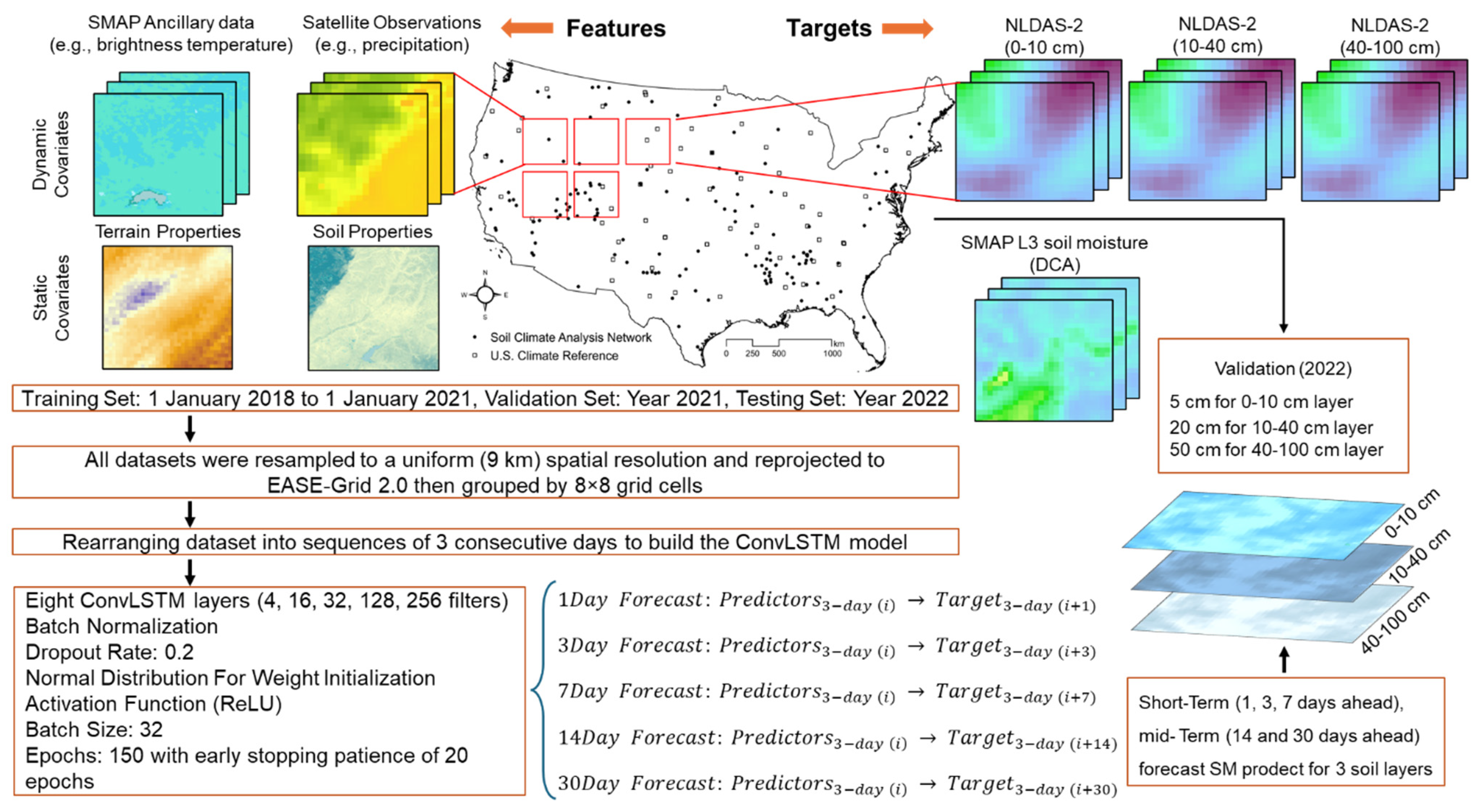
The architecture of the ConvLSTM model used in this study integrates convolutional operations directly within the LSTM units. Unlike traditional sequential models that apply CNN layers before LSTM layers (CNN-LSTM), the ConvLSTM architecture embeds convolutional filters within the internal gates of the LSTM itself. This design allows the model to learn both spatial features and temporal dependencies simultaneously, which is particularly effective for spatiotemporal forecasting of SM. Moreover, the model analyzes input data as three-dimensional tensors, which allows for capturing SM dynamics in space and in time and at different soil depths. Figure 2 displays an overview of the model workflow. Each input sample consists of a 3-day sequence of predictor variables extracted from an 8 × 8 spatial grid (~72 × 72 km area) using a stride of 2 to provide full spatial coverage across CONUS. While longer sequences could potentially improve predictive performance, they were avoided in this study to reduce computational costs and minimize the risk of overfitting, as pointed out in previous studies [26,44]. The final input tensor has the shape ‘samples, 8, 8, 3, 17’, where 8 × 8 represents the window size, 3 is the temporal look-back window (days), and 17 is the number of predictors used (see Table 2). The ConvLSTM network consists of eight hidden layers with filter sizes increasing progressively (4, 16, 32, 64, 128, and 256), followed by a fully connected output layer. Dropout layers were included between certain hidden layers to reduce overfitting by randomly deactivating a fraction of neurons during training. This patch-based input approach not only reduces memory requirements but also allows the model to learn localized fine-scale patterns across the spatial domain. Due to the large spatiotemporal extent of the dataset (five years of daily data across CONUS), automated hyperparameter tuning techniques such as grid search or Bayesian optimization were computationally impractical. Instead, a manual tuning strategy was used, in which key hyperparameters including the number of layers, filter sizes, dropout rates, and learning rates were iteratively tried within their typical ranges and modified based on model performance to obtain an optimal configuration.

Table 3. Summary of ConvLSTM Model Architecture and Key Hyperparameters Used for Large-Scale Soil Moisture Prediction.

Mosel Parameter	Value/Setting	Rationale
Hidden Layers	8	Capture hierarchical spatial-temporal features
Filter Sizes	4, 16, 32, 128, 256	Learn basic to complex patterns incrementally
Batch Normalization	After each ConvLSTM layer	Stabilize training, reduce covariate shift
Dropout Rate	0.2	Prevent overfitting in dense layers
Weight Initialization	Normal distribution	Enable efficient training with ReLU activations
Activation Function	ReLU	Introducing nonlinearity for complex mappings
Optimizer	Adam	Adaptive learning rate for faster convergence
Batch Size	32	Balance update stability and computational cost
Early Stopping Patience	20 epochs	Halt training if validation loss plateaus

summarizes the model’s hyperparameters, their optimal values and the rationale for their selection.

2.4. In Situ SM Data and Model Evaluation

To validate SM forecasts from the ConvLSTM model, we utilized in situ SM observations from the SCAN and USCRN that distributions among different land cover and soil classification are provided in

Table A1. Distribution of SCAN and USCRN soil moisture stations across major land cover types and soil texture classes at three depths (surface 0–10 cm, subsurface 10–40 cm, and subsurface 40–100 cm). Soil texture was classified according to the USDA soil texture classification scheme and grouped into coarse-textured (sand, loamy sand, and sandy loam), medium-textured (loam, clay loam, silt loam, sandy clay loam, silty clay loam, and silt), and fine-textured (clay, sandy clay, and silty clay) categories. Each cell entry is presented as X/Y, where X represents the number of stations in the SCAN and Y represents the number of stations in the USCRN.

Land Cover Type	Surface (0–10 cm)			Subsurface (10–40 cm)			Subsurface (40–100)
	Coarse	Medium	Fine	Coarse	Medium	Fine	Coarse	Medium	Fine
Grassland	20/6	22/13	0/4	5/3	36/19	1/1	8/4	32/18	2/1
Cropland	4/0	16/5	1/0	4/0	11/5	6/0	4/0	11/5	6/0
Permanent wetland	11/2	14/2	1/0	7/2	15/2	4/0	7/2	14/1	5/1
Savannas	17/8	13/5	1/0	10/5	18/7	3/1	7/5	21/6	3/2
Shrublands	5/4	4/8	0/0	4/1	5/11	0/0	3/1	6/10	0/2
Forest	5/0	2/1	0/0	3/0	3/1	1/0	4/0	2/1	1/0

SCAN: Soil Climate Analysis Network; USCRN: United States Climate Reference Network.

of Appendix A. SM observations were collected and quality-screened [45] from 137 SCAN and 59 USCRN stations, which are broadly distributed across diverse land cover types (Figure 1) and soil classes (

Table 4. Distribution of Soil Climate Analysis Network (SCAN) and U.S. Climate Reference Network (USCRN) soil moisture networks in different soil texture types across soil profile (n: the number of stations). The soil texture classification follows the USDA soil classification system.

Texture Class	Soil Texture	SCAN (N = 137)			USCRN (N = 59)
		Soil Layer (cm)			Soil Layer (cm)
		0–10	10–40	40–100	0–10	10–40	40–100
Coarse	Sand	2	2	2	1	2	1
	Loamy Sand	0	0	1	1	1	1
	Sandy Loam	60	31	30	23	8	10
Medium	Sandy Clay Loam	4	12	15	0	6	8
	Clay Loam	12	22	28	3	13	15
	Loam	17	28	23	13	11	9
	Silty Clay Loam	12	15	15	2	10	5
	Silt Loam	27	12	6	15	5	4
	Silt	0	0	0	0	0	0
Fine	Sandy Clay	0	0	0	0	0	0
	Silty Clay	3	5	6	1	0	3
	Clay	0	10	11	0	3	3

). Since SCAN and USCRN use different SM sensors and calibration methods, we conducted a separate evaluation for each network to account for potential discrepancies. Both networks provide SM observations at depths of 5, 10, 20, 50, and 100 cm. For evaluating surface SM, we used the 5 cm data, which aligns with SMAP and NLDAS-2 (0–10 cm) SM products. The 20 cm data used to validate subsurface SM corresponding to NLDAS-2 SM at 10–40 cm, while the 50 cm data used to evaluate deeper subsurface values corresponding to NLDAS-2 SM at 40–100 cm. The performance of the ConvLSTM-derived SM forecasts was evaluated using unseen data (test set) in 2022. To provide a robust evaluation of the ConvLSTM model, we used several error metrics: Pearson correlation coefficient (R), root mean squared error (RMSE), mean bias error (bias), and unbiased RMSE (ubRMSE), (Equations (9)–(12)) [46]. Among these, the ubRMSE is commonly used by the SMAP mission team to validate SM products by removing the effect of bias, with an acceptable ubRMSE value of up to 0.04 cm³ cm⁻³ [47].

$$R={\displaystyle \frac{\sum _{i=1}^n\left({\theta }_{{fcst}_i}-{\overline{\theta }}_{obs}\right)\left({\theta }_{{obs}_i}-{\overline{\theta }}_{obs}\right)}{\sqrt{\sum _{i=1}^n{\left({\theta }_{{fcst}_i}-{\overline{\theta }}_{obs}\right)}^2\sum _{i=1}^n{\left({\theta }_{{obs}_i}-{\overline{\theta }}_{fcst}\right)}^2}}}$$

(9)

$$RMSE=\sqrt{{\displaystyle \frac{1}{n}}\sum _{i=1}^{i=n}{({\theta }_{{fcst}_i}-{\theta }_{{obs}_i})}^2}$$

(10)

$$Bias={\displaystyle \frac{1}{n}}\sum _{i=1}^{i=n}({\theta }_{{fcst}_i}-{\theta }_{{obs}_i})$$

(11)

$$ubRMSE=\sqrt{{RMSE}^2-{Bias}^2}$$

(12)

where $n$ is the number of data; ${\theta }_{{fcst}_i}$ and ${\theta }_{{obs}_i}$ are the forecasted and observed SM values at time $i$, and ${\overline{\theta }}_{fcst}$ and ${\overline{\theta }}_{obs}$ are the corresponding mean values, ${\sigma }_{{\theta }_{fcst}}$ and ${\sigma }_{{\theta }_t}$ are the standard deviations of the forecasted and observed values, respectively.

3. Results and Discussion

We developed and validated a total of nine ConvLSTM models, in which three scenarios with different combinations of input predictors were considered for each soil layer (Table 2). The short- and mid-term forecasts were produced and validated for surface and subsurface soil layers, considering the effect of various soil textures and land cover types on the model performance, as detailed below.

3.1. Effect of Input Predictors on SM Nowcasting/Forecasting Accuracy

Table 5. Performance of ConvLSTM model for 1-day SM forecasts for three soil layers (0–10, 10–40, and 40–100 cm) evaluated under three scenarios of input predictors (S1, S2 and S3). Model outputs were compared with in situ SM from the SCAN (N = 137) and USCRN (N = 59) networks. For each layer and scenario, we repost the median and range (quartiles) of Pearson correlation (R), unbiased root mean square error (ubRMSE), and Bias. Bold values denote the scenario that yields the best performance for a given soil layer.

Network	Scenario	Soil Layer 0–10 cm
		R	ubRMSE	Bias
SCAN	S1	0.33, 0.58, 0.72	0.03, 0.045, 0.06	−0.07, −0.01, 0.06
	S2	0.442, 0.61, 0.73	0.02, 0.045, 0.06	−0.04, 0.01, 0.05
	S3	0.36, 0.58, 0.7	0.05, 0.07, 0.1	−0.05, −0.001, 0.06
USCRN	S1	0.42, 0.62, 0.75	0.038, 0.065, 0.075	−0.036, 0.007, 0.05
	S2	0.46, 0.61, 0.75	0.037, 0.064, 0.076	−0.026, 0.019, 0.044
	S3	0.38, 0.56, 0.69	0.036, 0.063, 0.075	−0.023, 0.014, 0.056
		Soil Layer 10–40 cm
		R	ubRMSE	Bias
SCAN	S1	0.12, 0.39, 0.69	0.027, 0.042, 0.056	−0.08, −0.003, 0.06
	S2	0.28, 0.59, 0.75	0.027, 0.04, 0.05	−0.08, −0.003, 0.06
	S3	0.33, 0.50, 0.64	0.028, 0.04, 0.055	−0.083, −0.008, 0.06
USCRN	S1	0.156, 0.47, 0.71	0.032, 0.05, 0.63	−0.045, −0.00, 0.05
	S2	0.31, 0.60, 0.79	0.030, 0.043, 0.06	−0.036, 0.001, 0.046
	S3	0.13, 0.52, 0.67	0.034, 0.048, 0.06	−0.026, 0.007, 0.046
		Soil Layer 40–100 cm
		R	ubRMSE	Bias
SCAN	S1	0.073, 0.46, 0.70	0.015, 0.032, 0.047	−0.13, −0.031, 0.054
	S2	0.16, 0.54, 0.73	0.02, 0.030, 0.045	−0.125, −0.033, 0.05
	S3	0.19, 0.52, 0.71	0.023, 0.032, 0.047	−0.12, −0.03, 0.04
USCRN	S1	0.41, 0.60, 0.73	0.018, 0.041, 0.068	−0.084, −0.012, 0.05
	S2	0.40, 0.63, 0.80	0.018, 0.037, 0.053	−0.075, −0.013, 0.05
	S3	0.39, 0.60, 0.77	0.02, 0.033, 0.049	−0.068, −0.007, 0.06

SCAN: Soil Climate Analysis Network; USCRN: U.S. Climate Reference Network; R: Pearson Correlation; ubRMSE: Unbiased Root Mean Square Error (cm³ cm⁻³); S1, S2 and S3: Scenarios 1, 2 and 3; values are quartile 1, quartile 2 (median) and quartile 3, respectively.

summarizes the ConvLSTM model performance for short-term (1-day lead time) forecasts at surface and subsurface depths in terms of median and interquartile ranges of R and ubRMSE values for each of the three input scenarios. Among these, scenario 2 (S2), which incorporated SMAP ancillary data and soil texture for layer and included upper-layer SM estimates for deeper layers (10–40 cm and 40–100 cm), outperformed the other S1 and S3 scenarios, confirming it as the best predictor combination. S2 incorporated SMAP ancillary data and soil texture for the surface layer and included upper-layer SM estimates to improve forecasts for the deeper layers (10–40 cm and 40–100 cm). These results indicate that the inclusion of soil texture information, as a major soil physical property, can improve the ability of the model to capture nonlinear spatiotemporal patterns of SM dynamics. This is in accordance with previous studies [39,48], which pointed out the importance of soil texture in near-surface SM modeling. For example, at the surface layer (0–10 cm), the median value of R over SCAN sites improved from 0.58 (S1 and S3 scenarios) to 0.61 under S2 scenario, while the median ubRMSE decreased from 0.07 (S3) to 0.045 cm³ cm⁻³ under S1 and S2.

A similar trend was observed for the two subsurface layers, with lower ubRMSE values (0.03 cm³ cm⁻³) and R values than that of surface layer (Table 5). Supporting this, Tahmouresi et al. [49] also reported a strong positive correlation between SMAP surface SM and the clay-to-sand content ratio, which indicates the value of soil texture in SM prediction. In subsurface layer (10–40 cm), the inclusion of upper layer SM estimates (i.e., 0–10 cm) in S2 notably improved the accuracy of SM nowcasts (i.e., 1-day lead time), where the median R value increased from 0.39 (S1) and 0.50 (S3) to 0.59 (S2), the median ubRMSE reduced from 0.042 (S1) to 0.04 cm³ cm⁻³ (S2 and S3), and the median bias improved from −0.008 (S3) to −0.003 cm³ cm⁻³ (S1 and S2). These results indicate the advantage of including upper-layer SM data to improve SM forecasts in deeper layers. Similar improvements were noted in the 40–100 cm layer. Comparable results were also obtained using USCRN data across all three soil layers scenarios (Table 5). The availability of SOLUS soil products, which provide high-resolution (100 m) maps of basic soil properties at multiple depths is advantageous for improving SM forecasts and downscaling SM products [50]. In this study, although the SOLUS-based soil texture maps (sand, silt and clay) were resampled from 100 m to 9 km grid, they still played an important role in improving SM forecasting at various depths.

Comparing the results from S2 and S3 indicates that including additional predictors does not necessarily improve model performance. This aligns with findings from prior studies, where reducing the number of input features through selection techniques like Lasso regularization improved model accuracy and generalization [51,52]. Interestingly, the inclusion of precipitation data in S3 did not improve the model performance. Although precipitation is the primary source of water input to the soil, its short-term signal does not always translate directly into measurable changes in soil moisture, particularly in deeper layers. The lag introduced by infiltration and percolation process often delays the response of SM to precipitation events [53]. As a potential improvement, future work could explore incorporating precipitation lag effects more explicitly, for example, by replacing daily precipitation inputs with aggregated 7-day or 14-day averages, as suggested by Heuvelink et al. [54]. Moreover, other dominant controls such as evapotranspiration, soil hydraulic properties, vegetation cover, and antecedent moisture conditions may exert stronger influences on SM dynamics that same-day precipitation. Another contributing factor may be the scale mismatch, as precipitation datasets typically have coarser spatial resolution and higher uncertainty compared to SM and other predictors. Consistent with this observation, Karthikeyan and Mishra [55] reported that precipitation contributed least to SM prediction across all depths in feature importance analysis. Given that Scenario 2 produced more accurate short-term forecasts for both surface and subsurface layers, we relied on Scenario 2 to present the ConvLSTM model results in the following sections.

3.2. Short- and Mid-Term Surface and Subsurface SM Forecasts

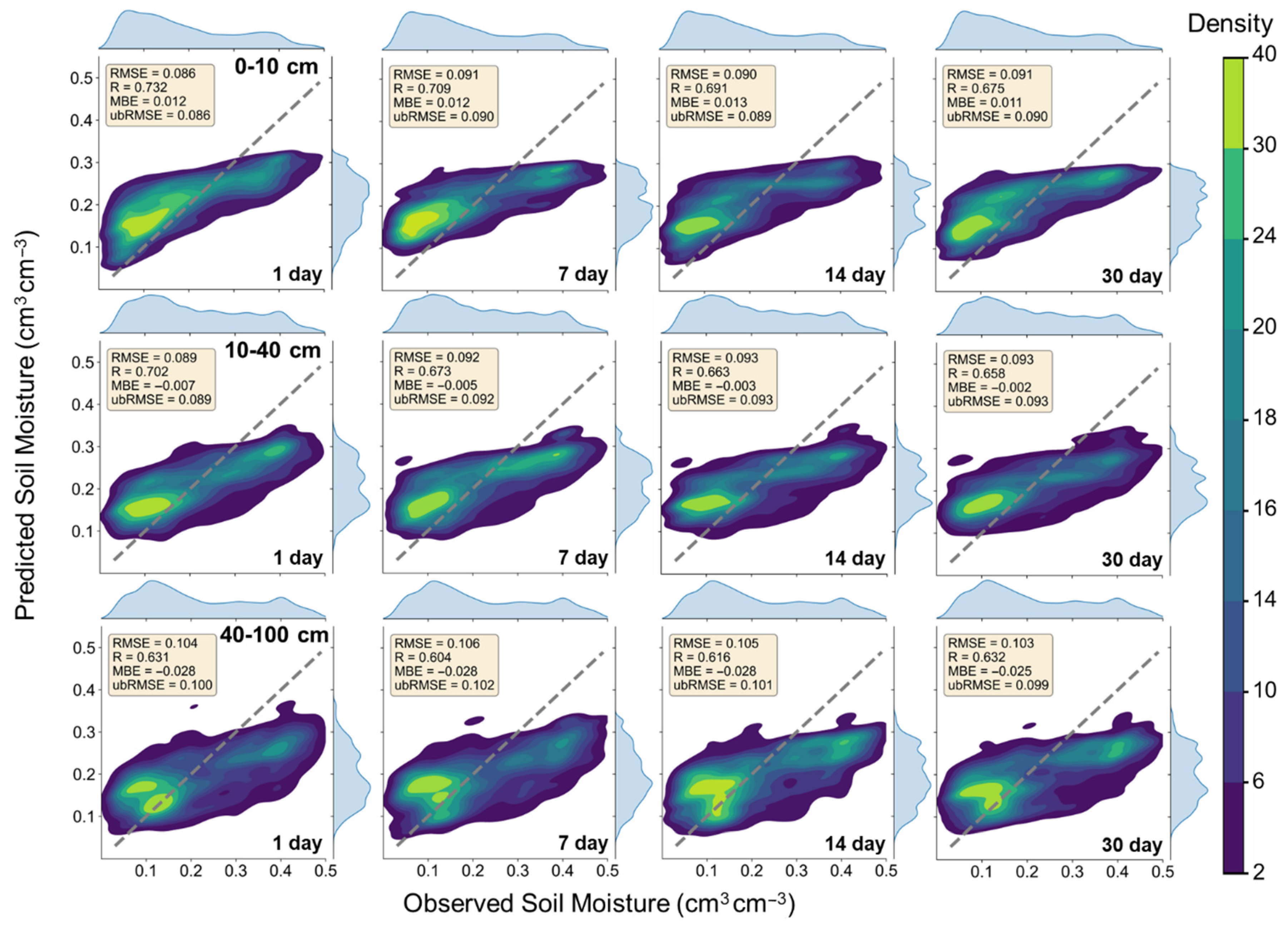
Building upon the results that the S2 scenario provided the highest accuracy for 1-day forecasts at the three soil layers for SCAN and USCRN, we further evaluated its performance for short- (1 and 7 days) and mid-term (14 and 30 days) forecast lead times. Figure 3 depicts the evaluation of S2 scenario forecasts using in situ observations from SCAN sites for the year 2022. Because the model performance using USCRN data yielded error metrics comparable to those from SCAN sites, the detailed results from USCRN are provided separately in Figure A1 (Appendix A). Results indicated that the accuracy of SM forecast decreased with increasing lead time across all depths. This decline was most pronounced in the surface (0–10 cm) and subsurface (10–40 cm) layers, where SM is highly dynamic due to rapid responses to rainfall inputs and evapotranspiration losses. These processes introduce large short-time fluctuations, making predictions at longer lead times more uncertain. The scatterplots show that the ConvLSTM model maintains relatively high accuracy across all three soil layers with the best accuracy at 1-day lead time. For example, at the surface layer (0–10 cm), the model achieves an ubRMSE of 0.086 cm³ cm⁻³ and R of 0.73 for 1-day lead time. The accuracy declined slightly in 7 days with ubRMSE of 0.090 cm³ cm⁻³ and R of 0.71. Similar trends were observed for the subsurface layers. At 10–40 cm, the ubRMSE increased from 0.089 (1-day) to 0.093 cm³ cm⁻³ (30-day) and R decreased from 0.70 (1-day) to 0.66 (30-day).

A systematic bias was observed across depths and lead times, where the model tended to over-forecast SM under dry conditions (~less than 0.10 cm³ cm⁻³) and under-forecast under wet conditions (~higher than 0.35 cm³ cm⁻³). This pattern can be attributed to several factors. First, spatial mismatches arise when comparing gridded forecasts (9 km pixel size) to point-scale in situ values [1]. Second, vertical mismatches occur because the model provides average SM over thick layers (e.g., 0–10 cm), whereas in situ sensors provide data at more discrete depths (e.g., 5, 20, and 50 cm), which may not fully capture the entire modeled layer. Third, the ConvLSTM architecture uses a hyperbolic tangent (tanh) activation function for the memory cells and a sigmoid function for gate operations. While this setup ensures physically consistent outputs (e.g., preventing negative values), it may also compress extreme values toward the mean, which can lead to under-forecasting of SM in high moisture conditions [56]. Moreover, considering the 9 km spatial resolution of the forecasts, extremely dry or wet conditions are unlikely to be uniformly present across the entire grid cell. Therefore, the model’s relatively smooth responses reflect not only a limitation of the architecture but also the inherent physical averaging effects at coarser resolutions.

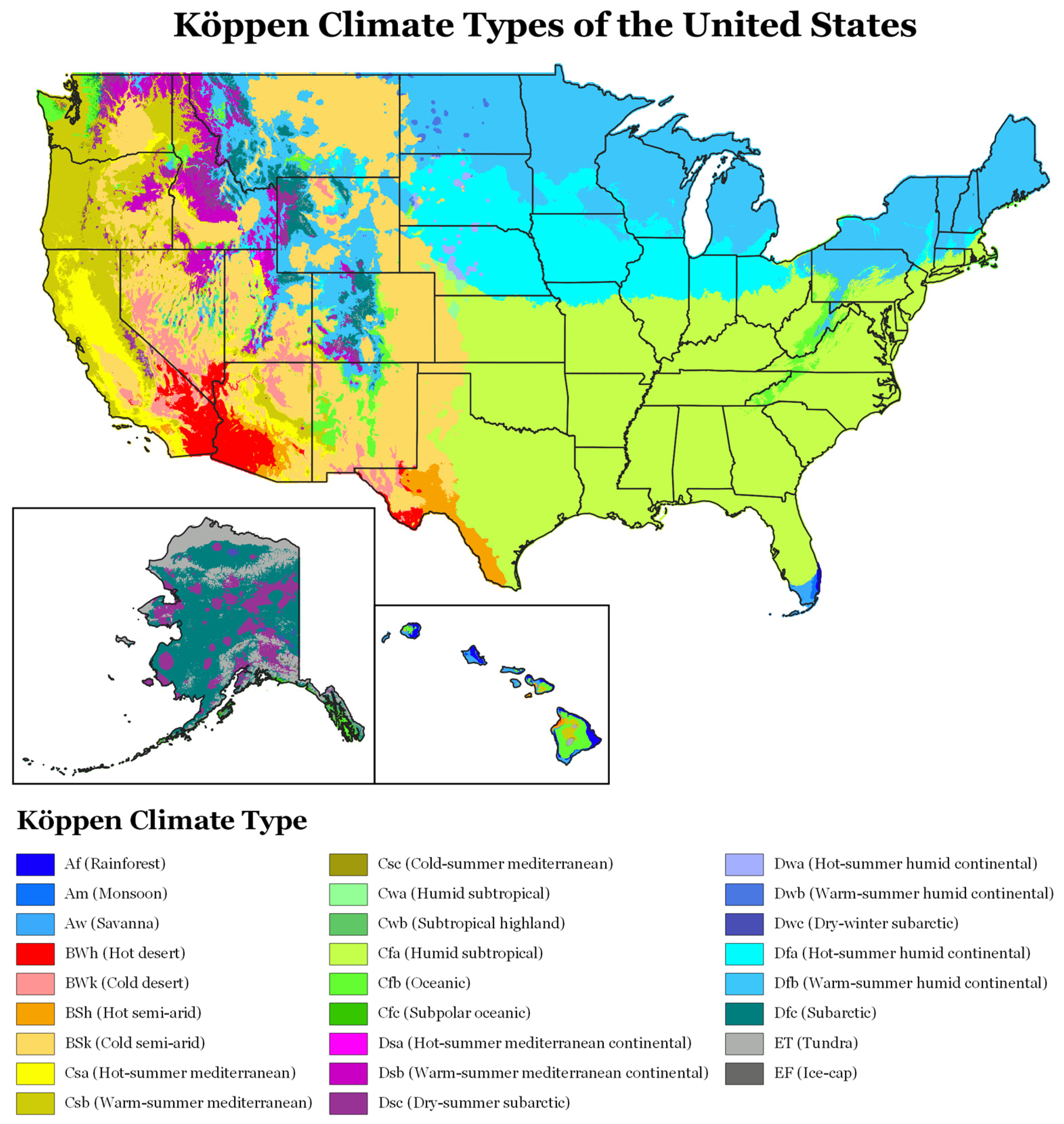
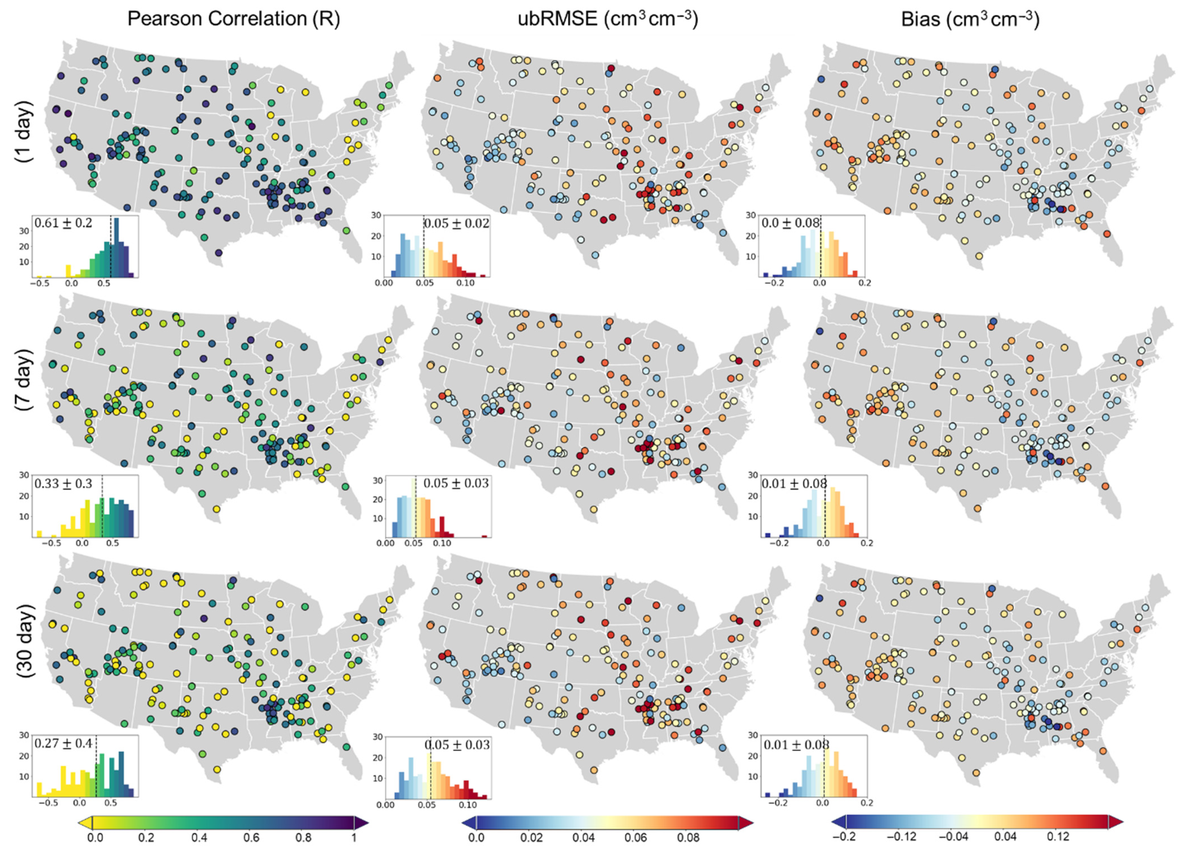
The performance of the ConvLSTM model (test set) based on the test set for short- (1-, and 7-day) and mid-term (30-day) SM forecasts across the three layers based on the S2 scenario are depicted in Figure 4, Figure 5 and Figure 6 for all SCAN and USCRN sites. As shown in Figure 4, for the 0–10 cm layer, both short- and mid-term forecasts showed median ubRMSE and bias values of 0.05 cm³ cm⁻³ and 0.01 cm³ cm⁻³, respectively. Unsurprisingly, the R values declined with increasing the forecast lead time, ranging from 0.27 (30-day) to 0.61 (1-day). The largest ubRMSE and bias values were observed in the Mideast and Southeast regions, although the corresponding R values remained relatively high. This finding is consistent with Karthikeyan and Mishra ([55], Figure 5) who reported that at 5 cm and 10 cm depths, ubRMSE was high (~0.06 cm³ cm⁻³) while correlation was also strong (~0.8). Such behavior can be attributed to pronounced soil moisture fluctuations in these regions (see Figure 6 in [57]). As a result, the model was able to capture the overall temporal pattern of soil moisture dynamics (e.g., wet and dry seasons) but less accurately estimated the exact magnitudes. In contrast, the Northeast showed lower R values and higher ubRMSE values, likely due to the effect of dense vegetation which interferes with SMAP brightness temperature observations, and the narrower range of SM variations which weaken the R values. In addition, frequent freeze–thaw cycles and seasonal snowpack in the northeast reduce temporal data quality and increase ubRMSE.

Similar spatial patterns in SM accuracy have been reported by Fang et al. ([58], Figure 1) who used an LSTM model to assimilate SMAP level 3 data for SM mapping. Another example is the work by Karthikeyan and Mishra ([55], Figure 5) in which they generated 1 km SM maps across the U.S. In terms of ubRMSE and R values, the best SM forecasts were obtained in the Southwest and parts of the West, where sparse vegetation and lower vegetation water content reduce signal interference. Notably, SM forecast errors were particularly low at stations located in Utah state. Unlike SMAP SM products, which often show low accuracy in this region due to the influence of snowpack and complex mountainous terrain [59], the ConvLSTM model demonstrated high accuracy in both R and ubRMSE values. This improved performance may be attributed to integrating the strengths of the two different SM products from the physics-based SMAP L3 (DCA), which uses surface observations, and a process-based model (NLDAS-2), which considers hydrological processes. In addition, in the northeastern CONUS, the forecast performance at the surface layer (0–10 cm) was relatively poor, with correlation values (R) ranging from −0.3 to 0.2 and ubRMSE values ranging from 0.07 to 0.11 cm³ cm⁻³ (Figure 4). This reduced accuracy can be attributed to the prevailing cold and humid continental climate (Dfa/Dfb classes in the Köppen classification, Figure A2), where soil freezing is common during winter months. Frozen soils alter the dielectric properties sensed by satellites and strongly affect the dynamics of soil moisture, leading to discrepancies between modeled forecasts and in situ measurements. These freeze–thaw processes introduce nonlinear and abrupt changes that are challenging for data-driven models to capture, thereby reducing forecast skill in this region. For the surface layer (0–10 cm), nearly 50% of the evaluated SM stations (90 sites) achieved ubRMSE values below the SMAP accuracy threshold of 0.04 cm³ cm⁻³ [47] for both short- and mid-term SM forecasts.

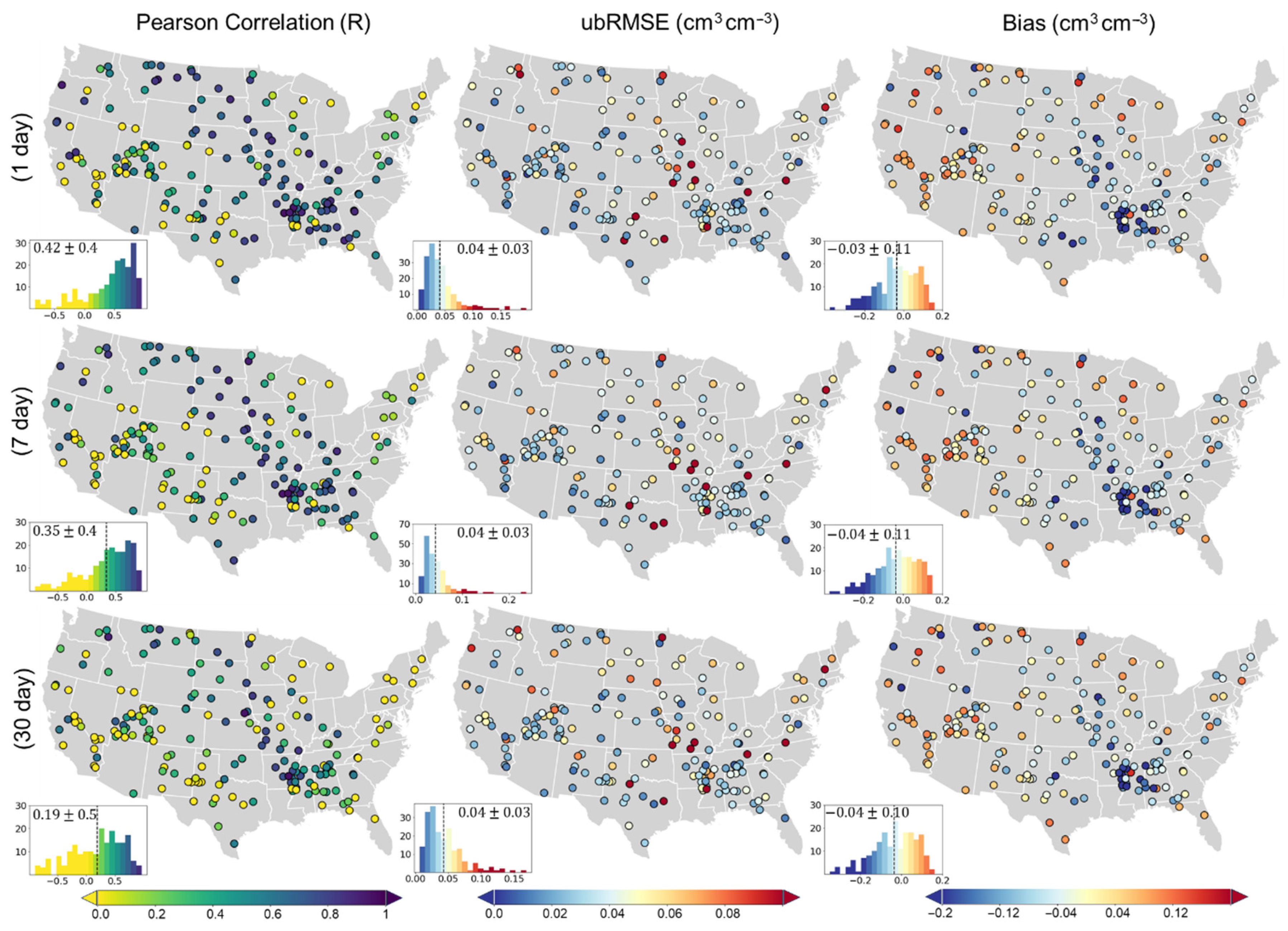
Results for the subsurface layers (10–40 cm and 40–100 cm) followed similar trends to the surface layer. Overall, R values decreased with increasing forecasting lead time, while ubRMSE values slightly increased. For the 10–40 cm layer, mean R values ranged from 0.22 (30-day lead time) to 0.59 (1-day lead time), while the ubRMSE values ranged from 0.04 (1-day lead time) to 0.05 cm³ cm⁻³ (30-day lead time). The bias values were similar to those obtained for 0–10 cm layer. For the 40–100 cm layer, R values ranged from 0.19 (30-day lead time) to 0.42 (1-day lead time), while ubRMSE values achieved 0.04 cm³ cm⁻³ across all three lead times. The lower R values at greater layers may be due to the limited sensitivity of the input predictors (except soil texture data), especially satellite-derived features, to subsurface conditions (depth greater than 5 cm). Still, the model achieved the SMAP accuracy target of 0.04 cm³ cm⁻³ at over 50% of the sites for both 10–40 cm and 40–100 cm layers.

3.3. SM Forecasts Under Different Land Cover Types

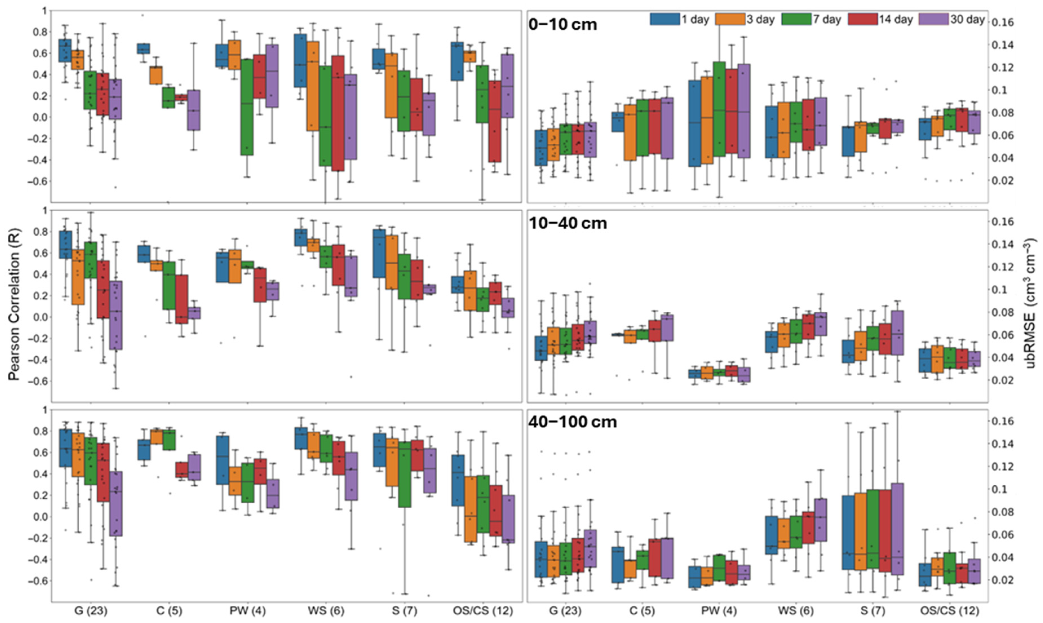
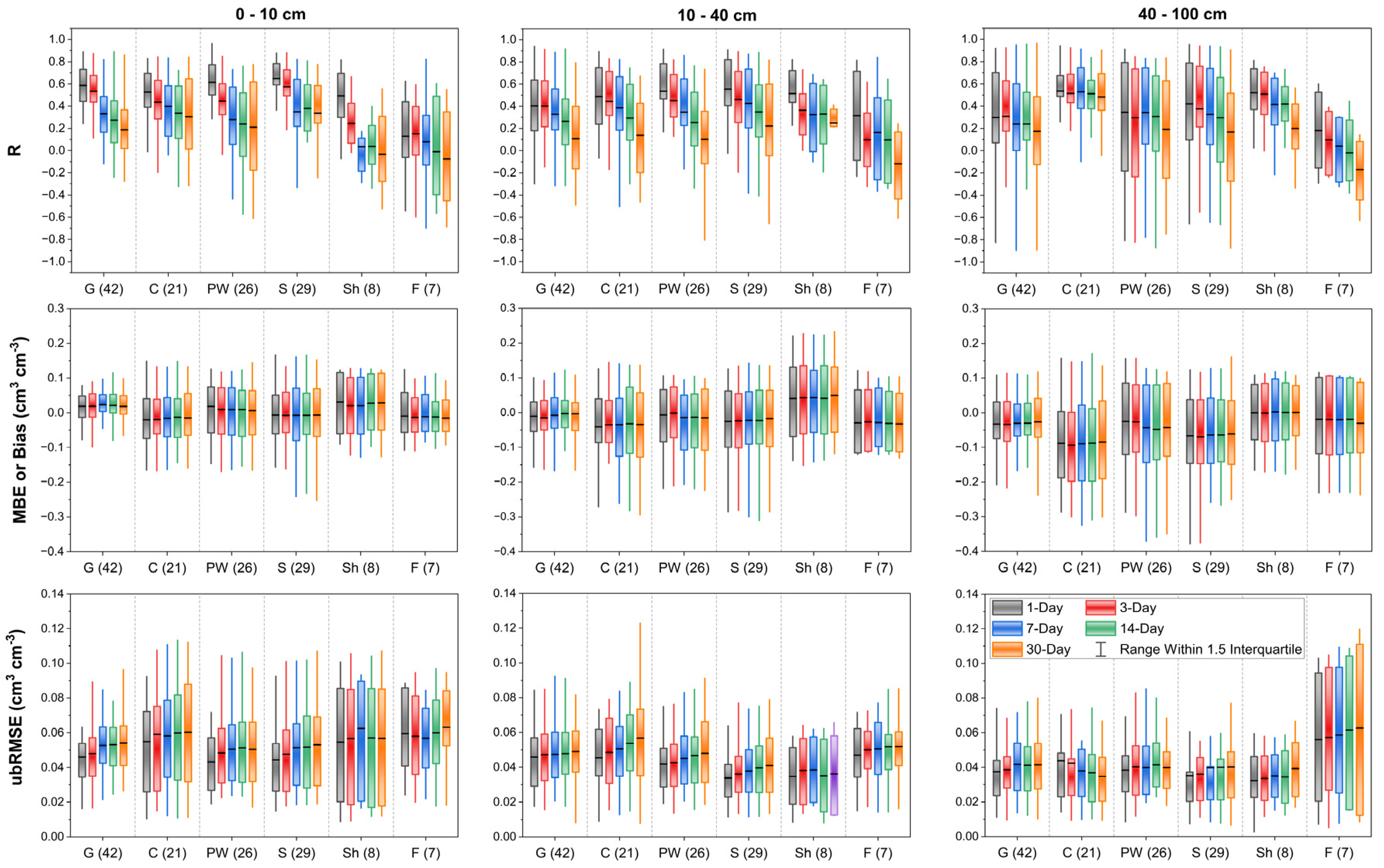
Figure 7 depicts the model performance (test set) for the S2 scenario at three soil layers at SCAN sites under six dominant land cover types. Overall, the accuracy of SM forecasts, shown by R, ubRMSE and bias, decreases with increasing forecast lead time, which is in accordance with previous studies [16]. When examined across land cover types, the ConvLSTM model generally performed best in grasslands and savannas, where SM variability is more directly linked to precipitation and evapotranspiration cycles, resulting in higher correlation coefficients (R), but sometimes greater bias and ubRMSE. In contrast, forests and shrublands exhibited lower accuracy, likely due to the buffering effect of dense vegetation and complex canopy-soil interactions, which obscure direct precipitation-soil moisture relationships. Croplands and permanent water bodies showed intermediate errors, with higher variability across SCAN sites. For the 0–10 cm layer, the model achieved median ubRMSE values below 0.06 cm³ cm⁻³ and median R values ranging approximately from 0.05 to 0.65 for all lead times and land cover types. Generally, in terms of R, the accuracy of SM forecasts decreased with increasing soil depth, whereas ubRMSE values improved with depth. To better explore in all lead times and land cover types, the median R values ranged from 0.10 to 0.55, while the median ubRMSE values were below 0.05 and 0.04 cm³ cm⁻³ for the 10–40 cm and 40–100 cm layers, respectively. These results indicate a significant improvement compared to previous studies. For example, Tavakol et al. [12] reported daily ubRMSE values greater than 0.12 cm³ cm⁻³ for SMAP L3 across the U.S. between April 2015 and November 2017, with values of 0.11, 0.12, and 0.09 cm³ cm⁻³ for grasslands, croplands, and shrublands, respectively (see Table 2 in [12]). Similarly, Xing et al. [60] found Spearman correlation values of approximately 0.50 over grassland, 0.55 over croplands, and 0.45 over forested. Yi et al. [61] reported Pearson correlation values of 0.41, 0.60, and 0.45 for the same land cover types, respectively. Comparable performance trends were observed using USCRN SM observations, as shown in Figure A3 (Appendix A).

3.4. SM Forecasts Under Different Soil Textures

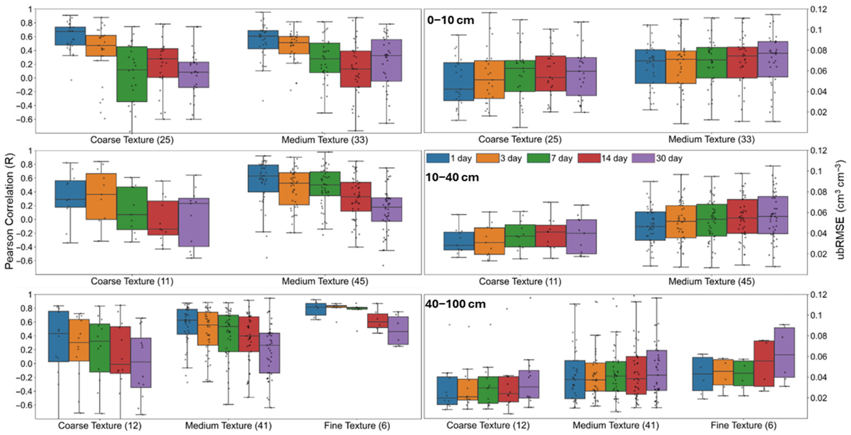
Figure 8 displays the performance of the S2 scenario for SM forecasts across three broad soil textural classes: coarse-textured (sand, loamy sand, and sandy loam), medium-textured (loam, clay loam, silt loam, sandy clay loam, silty clay loam, silt), and fine-textured (sandy clay, silty clay, and clay) soils for three soil layers (0–10 cm, 10–40 cm, and 40–100 cm) and five lead times (1-, 3-, 7-, 14-, and 30-day) across SCAN sites (test set). Results showed that forecast accuracy was highest in coarse-textured soils, which allow rapid infiltration and clearer SM responses to precipitation, leading to relatively higher R values and lower errors. Medium-textured soils showed intermediate performance, while fine-textured soils exhibited the greatest challenges, particularly at deeper layers (40–100 cm), where slower infiltration and stronger retention effects delay the SM responses, reducing forecast skill over longer lead times. In terms of ubRMSE values at the surface layer (0–10 cm), coarse-textured soils showed the lowest errors for all lead times, followed by medium- and fine-textured soils. However, the ranking was different for R, where medium-textured soils outperformed fine- and coarse-textured soils. These differences may be partly explained by soil hydraulic properties, i.e., sandy soils have high infiltration capacity and rapid percolation rates, leading to rapid SM responses to rainfall but also faster drying, which can reduce temporal correlation. Conversely, fine-textured soils with low infiltration capacity can generate surface runoff during high precipitation rates, delaying water movement into deeper layers and dampening SM variability, thereby affecting R and ubRMSE. Additionally, the rapid SM fluctuations in sandy soils may increase the effective sensing depth of SMAP [62,63], affecting forecast performance patterns in various textures. The median bias was generally near zero across all soil textures and soil layers; however, slightly larger deviations were noted in the deeper layers for medium and fine-textured soils. These biases likely reflect challenges in capturing infiltration and redistribution processes in these two major soil textural classes where water moves slowly within the soil profile which slows down wetting-drying cycles. Similar performance patterns were observed using USCRN SM observations, as shown in Figure A4 (Appendix A).

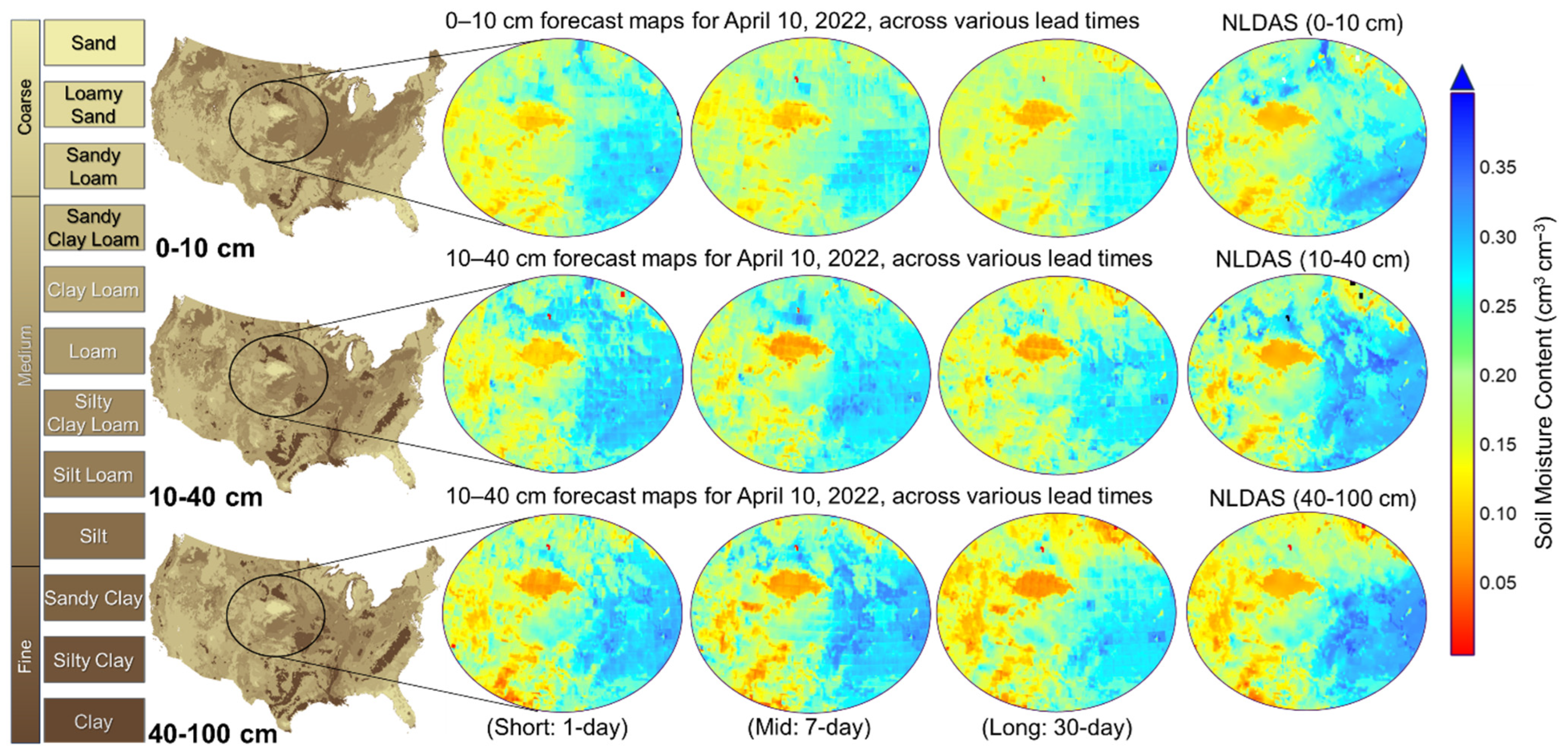
3.5. Short- and Mid-Term SM Forecast Maps

To evaluate the performance of ConvLSTM model under the S2 scenario for producing spatiotemporal SM maps, we produced forecast maps for 10 April 2022 across three soil layers with lead times of 1, 7, and 30 days (Figure 9). These forecasted maps were visually compared with NLDAS-2 SM product for the corresponding layers, along with underlying soil texture data from the SOLUS100 digital soil maps. Across all three layers, the model forecasts closely matched the spatial patterns observed in the NLDAS-2 maps. The model successfully captured drier SM distributions in sandy regions and higher moisture levels in finer-textured soils, such as those found in the Midwest and Southeast. Notably, areas dominated by sandy soils, like Nebraska, showed lower SM values in both the forecasts and NLDAS-2, while clay- or silty-rich regions, like the lower Mississippi basin, showed higher moisture retention [49,59]. This strong spatial correspondence demonstrates the ability of the ConvLSTM model to reflect the effect of soil texture on water retention, storage, and infiltration. As the forecast lead time increases from 1 to 30 days, a gradual loss of fine-scale spatial detail becomes evident, especially in deeper soil layers, which indicates growing uncertainty with longer lead times. Nevertheless, even at 30-day lead time, the forecasts show general spatial agreement with the NLDAS-2 product, especially in subsurface layers.

4. Summary and Conclusions

Accurate real-time soil moisture (SM) information is essential for a wide range of Earth and environmental science applications. This study presents a deep learning framework for forecasting SM at short- (1, 3, and 7 days) and mid-term (14 and 30 days) time scales for surface (0–10 cm) and subsurface (10–40 cm and 40–100 cm) layers across the contiguous U.S. The model integrates multiple data sources including SMAP L3 SM and its ancillary variables (e.g., brightness temperature, surface temperature), NLDAS-2 SM products, SOLUS100 soil property maps, MODIS observations, terrain attributes, precipitation, and upper-layer SM information. The forecasting framework combines convolutional neural network and long short-term memory networks trained with multi-year datasets. This integration improved the ability to capture both spatial and temporal patterns of SM dynamics at a large scale. We evaluated three scenarios with different combinations of input features. The produced SM forecasts at multiple soil layers were evaluated with in situ observations from SCAN and USCRN, which covered various land cover and soil types.

The results indicate that the accuracy of SM forecasts declines with increasing lead time. For surface SM, the median ubRMSE remained below 0.06 cm³ cm⁻³. Including SOLUS100-based soil physical properties and upper-layer SM as an additional predictor improved subsurface forecasts. The median R values were nearly 0.61 (surface) and 0.60 (10–40 cm), with median ubRMSE less than 0.045 cm³ cm⁻³. Integrating SMAP L3 (dual-channel algorithm) data with NLDAS-2 SM products yielded SM forecasts that met the SMAP accuracy target (ubRMSE ~0.04 cm³ cm⁻³) at more than half of the SCAN sites. For lead times of 1 to 30 days, median ubRMSE values were below 0.06 cm³ cm⁻³ with R values ranging from 0.19 (30-day) to around 0.66 (1-day). The accuracy varied by land cover type, where grasslands and savannas yielded the best accuracy, while dense forests and shrublands reduced the accuracy due to vegetation attenuation and complex hydrological processes. The soil texture also affected the accuracy of SM forecasts, with coarse-textured soils showing the lowest ubRMSE for all lead times, followed by medium and fine textures. Forecast errors tended to overestimate in dry and underestimate in wet extremes, likely due to grid-to-point scale mismatches and differences between depth-averaged model outputs vs. point-based observations. The forecast maps captured spatial patterns similar to NLDAS-2 SM and showed consistent patterns with soil texture even at the 30-day lead time, which indicates the ability of the model to identify spatial patterns of SM even at a large scale.

One limitation of the current study is that in situ soil moisture observations were not directly included in the training phase. Instead, the model was trained to minimize MSE against the SMAP soil moisture product and to follow the soil moisture patterns provided by the NLDAS-2 product. For future research directions, it is suggested that in situ SM observations be incorporated into the training process to reduce scale mismatch biases. Optimizing ConvLSTM model hyperparameters using advanced methods (e.g., Bayesian optimization) and exploring ensemble or transformer-based spatiotemporal architectures may improve forecast accuracy. Another limitation is the spatial resolution of the produced product, which remains at 9 km (similar to SMAP), thereby limiting its applicability for field-scale uses such as precision agriculture. Producing high-resolution maps of SM nowcasts and forecasts by incorporating higher resolution satellites (e.g., Sentinel group) [64] can support agricultural water management and drought and flood monitoring and mitigation.

References

1. Babaeian, E.; Sadeghi, M.; Jones, S.B.; Montzka, C.; Vereecken, H.; Tuller, M. Ground, Proximal, and Satellite Remote Sensing of Soil Moisture. Rev. Geophys. 2019, 57, 530–616. [Google Scholar] [CrossRef]
2. Seneviratne, S.I.; Corti, T.; Davin, E.L.; Hirschi, M.; Jaeger, E.B.; Lehner, I.; Orlowsky, B.; Teuling, A.J. Investigating soil moisture–climate interactions in a changing climate: A review. Earth-Sci. Rev. 2010, 99, 125–161. [Google Scholar] [CrossRef]
3. Koster, R.D.; Mahanama, S.P.P.; Yamada, T.J.; Balsamo, G.; Berg, A.A.; Boisserie, M.; Dirmeyer, P.A.; Doblas-Reyes, F.J.; Drewitt, G.; Gordon, C.T.; et al. Contribution of land surface initialization to subseasonal forecast skill: First results from a multi-model experiment. Geophys. Res. Lett. 2010, 37, L02402. [Google Scholar] [CrossRef]
4. Sheffield, J.; Wood, E.F. Global Trends and Variability in Soil Moisture and Drought Characteristics, 1950–2000, from Observation-Driven Simulations of the Terrestrial Hydrologic Cycle. J. Clim. 2008, 21, 432–458. [Google Scholar] [CrossRef]
5. Brocca, L.; Ciabatta, L.; Massari, C.; Moramarco, T.; Hahn, S.; Hasenauer, S.; Kidd, R.; Dorigo, W.; Wagner, W.; Levizzani, V. Soil as a natural rain gauge: Estimating global rainfall from satellite soil moisture data. J. Geophys. Res. Atmos. 2014, 119, 5128–5141. [Google Scholar] [CrossRef]
6. Zhao, B.; Dai, Q.; Zhuo, L.; Zhu, S.; Shen, Q.; Han, D. Assessing the potential of different satellite soil moisture products in landslide hazard assessment. Remote Sens. Environ. 2021, 264, 112583. [Google Scholar] [CrossRef]
7. Myoung, B.; Kim, S.; Nghiem, S.; Jia, S.; Whitney, K.; Kafatos, M. Estimating Live Fuel Moisture from MODIS Satellite Data for Wildfire Danger Assessment in Southern California USA. Remote Sens. 2018, 10, 87. [Google Scholar] [CrossRef]
8. Western, A.W.; Grayson, R.B.; Blöschl, G. Scaling of Soil Moisture: A Hydrologic Perspective. Annu. Rev. Earth Planet. Sci. 2002, 30, 149–180. [Google Scholar] [CrossRef]
9. Jackson, T.J.; Hsu, A.Y.; O’Neill, P.E. Surface Soil Moisture Retrieval and Mapping Using High-Frequency Microwave Satellite Observations in the Southern Great Plains. J. Hydrometeorol. 2002, 3, 688–699. [Google Scholar] [CrossRef]
10. Entekhabi, D.; Njoku, E.G.; O’Neill, P.E.; Kellogg, K.H.; Crow, W.T.; Edelstein, W.N.; Entin, J.K.; Goodman, S.D.; Jackson, T.J.; Johnson, J.; et al. The Soil Moisture Active Passive (SMAP) Mission. Proc. IEEE 2010, 98, 704–716. [Google Scholar] [CrossRef]
11. Reichle, R.H.; Liu, Q.; Koster, R.D.; Crow, W.T.; De Lannoy, G.J.M.; Kimball, J.S.; Ardizzone, J.V.; Bosch, D.; Colliander, A.; Cosh, M.; et al. Version 4 of the SMAP Level-4 Soil Moisture Algorithm and Data Product. J. Adv. Model. Earth Syst. 2019, 11, 3106–3130. [Google Scholar] [CrossRef]
12. Tavakol, A.; Rahmani, V.; Quiring, S.M.; Kumar, S.V. Evaluation analysis of NASA SMAP L3 and L4 and SPoRT-LIS soil moisture data in the United States. Remote Sens. Environ. 2019, 229, 234–246. [Google Scholar] [CrossRef]
13. ECMWF. IFS Documentation CY41R2—Part IV: Physical Processes. In IFS Documentation CY41R2; ECMWF: Reading, UK, 2016. [Google Scholar]
14. Filipović, N.; Brdar, S.; Mimić, G.; Marko, O.; Crnojević, V. Regional soil moisture prediction system based on Long Short-Term Memory network. Biosyst. Eng. 2022, 213, 30–38. [Google Scholar] [CrossRef]
15. ElSaadani, M.; Habib, E.; Abdelhameed, A.M.; Bayoumi, M. Assessment of a Spatiotemporal Deep Learning Approach for Soil Moisture Prediction and Filling the Gaps in Between Soil Moisture Observations. Front. Artif. Intell. 2021, 4, 636234. [Google Scholar] [CrossRef] [PubMed]
16. Ahmed, A.A.M.; Deo, R.C.; Raj, N.; Ghahramani, A.; Feng, Q.; Yin, Z.; Yang, L. Deep Learning Forecasts of Soil Moisture: Convolutional Neural Network and Gated Recurrent Unit Models Coupled with Satellite-Derived MODIS, Observations and Synoptic-Scale Climate Index Data. Remote Sens. 2021, 13, 554. [Google Scholar] [CrossRef]
17. Datta, P.; Faroughi, S.A. A multihead LSTM technique for prognostic prediction of soil moisture. Geoderma 2023, 433, 116452. [Google Scholar] [CrossRef]
18. Seo, M.-G.; Shin, H.-S.; Tsourdos, A. Soil Moisture Retrieval from Airborne Multispectral and Infrared Images using Convolutional Neural Network. IFAC-PapersOnLine 2020, 53, 15852–15857. [Google Scholar] [CrossRef]
19. Sadeghi, M.; Asanjan, A.A.; Faridzad, M.; Nguyen, P.; Hsu, K.; Sorooshian, S.; Braithwaite, D. PERSIANN-CNN: Precipitation Estimation from Remotely Sensed Information Using Artificial Neural Networks–Convolutional Neural Networks. J. Hydrometeorol. 2019, 20, 2273–2289. [Google Scholar] [CrossRef]
20. Li, Y.; Wang, W.; Wang, G.; Tan, Q. Actual evapotranspiration estimation over the Tuojiang River Basin based on a hybrid CNN-RF model. J. Hydrol. 2022, 610, 127788. [Google Scholar] [CrossRef]
21. Han, J.; Shi, L.; Yang, Q.; Chen, Z.; Yu, J.; Zha, Y. Rice yield estimation using a CNN-based image-driven data assimilation framework. Field Crop. Res. 2022, 288, 108693. [Google Scholar] [CrossRef]
22. Hochreiter, S.; Schmidhuber, J. Long Short-Term Memory. Neural Comput. 1997, 9, 1735–1780. [Google Scholar] [CrossRef]
23. Fang, K.; Shen, C. Near-Real-Time Forecast of Satellite-Based Soil Moisture Using Long Short-Term Memory with an Adaptive Data Integration Kernel. J. Hydrometeorol. 2020, 21, 399–413. [Google Scholar] [CrossRef]
24. Shi, X.; Chen, Z.; Wang, H.; Yeung, D.-Y.; Wong, W.; Woo, W. Convolutional LSTM Network: A Machine Learning Approach for Precipitation Nowcasting. Adv. Neural Inf. Process. Syst. 2015, 28. [Google Scholar] [CrossRef]
25. Babaeian, E.; Paheding, S.; Siddique, N.; Devabhaktuni, V.K.; Tuller, M. Short- and mid-term forecasts of actual evapotranspiration with deep learning. J. Hydrol. 2022, 612, 128078. [Google Scholar] [CrossRef]
26. Huang, F.; Zhang, Y.; Zhang, Y.; Shangguan, W.; Li, Q.; Li, L.; Jiang, S. Interpreting Conv-LSTM for Spatio-Temporal Soil Moisture Prediction in China. Agriculture 2023, 13, 971. [Google Scholar] [CrossRef]
27. Lamichhane, M.; Mehan, S.; Mankin, K.R. Soil Moisture Prediction Using Remote Sensing and Machine Learning Algorithms: A Review on Progress, Challenges, and Opportunities. Remote Sens. 2025, 17, 2397. [Google Scholar] [CrossRef]
28. Fang, K.; Pan, M.; Shen, C. The Value of SMAP for Long-Term Soil Moisture Estimation with the Help of Deep Learning. IEEE Trans. Geosci. Remote Sens. 2019, 57, 2221–2233. [Google Scholar] [CrossRef]
29. Xia, Y.; Sheffield, J.; Ek, M.B.; Dong, J.; Chaney, N.; Wei, H.; Meng, J.; Wood, E.F. Evaluation of multi-model simulated soil moisture in NLDAS-2. J. Hydrol. 2014, 512, 107–125. [Google Scholar] [CrossRef]
30. Gao, L.; Ebtehaj, A.; Chaubell, M.J.; Sadeghi, M.; Li, X.; Wigneron, J.-P. Reappraisal of SMAP inversion algorithms for soil moisture and vegetation optical depth. Remote Sens. Environ. 2021, 264, 112627. [Google Scholar] [CrossRef]
31. Hou, A.Y.; Kakar, R.K.; Neeck, S.; Azarbarzin, A.A.; Kummerow, C.D.; Kojima, M.; Oki, R.; Nakamura, K.; Iguchi, T. The Global Precipitation Measurement Mission. Bull. Am. Meteorol. Soc. 2014, 95, 701–722. [Google Scholar] [CrossRef]
32. Adirosi, E.; Montopoli, M.; Bracci, A.; Porcù, F.; Capozzi, V.; Annella, C.; Budillon, G.; Bucchignani, E.; Zollo, A.L.; Cazzuli, O.; et al. Validation of GPM Rainfall and Drop Size Distribution Products through Disdrometers in Italy. Remote Sens. 2021, 13, 2081. [Google Scholar] [CrossRef]
33. Nauman, T.W.; Kienast-Brown, S.; Roecker, S.M.; Brungard, C.; White, D.; Philippe, J.; Thompson, J.A. Soil landscapes of the United States (SOLUS): Developing predictive soil property maps of the conterminous United States using hybrid training sets. Soil Sci. Soc. Am. J. 2024, 88, 2046–2065. [Google Scholar] [CrossRef]
34. Minár, J.; Evans, I.S.; Jenčo, M. A comprehensive system of definitions of land surface (topographic) curvatures, with implications for their application in geoscience modelling and prediction. Earth-Sci. Rev. 2020, 211, 103414. [Google Scholar] [CrossRef]
35. Crow, W.T.; Berg, A.A.; Cosh, M.H.; Loew, A.; Mohanty, B.P.; Panciera, R.; de Rosnay, P.; Ryu, D.; Walker, J.P. Upscaling sparse ground-based soil moisture observations for the validation of coarse-resolution satellite soil moisture products. Rev. Geophys. 2012, 50, RG200. [Google Scholar] [CrossRef]
36. Sadeghi, M.; Jones, S.B.; Philpot, W.D. A linear physically-based model for remote sensing of soil moisture using short wave infrared bands. Remote Sens. Environ. 2015, 164, 66–76. [Google Scholar] [CrossRef]
37. Mokhtari, A.; Sadeghi, M.; Afrasiabian, Y.; Yu, K. OPTRAM-ET: A novel approach to remote sensing of actual evapotranspiration applied to Sentinel-2 and Landsat-8 observations. Remote Sens. Environ. 2023, 286, 113443. [Google Scholar] [CrossRef]
38. Friedl, M.A.; Sulla-Menashe, D.; Tan, B.; Schneider, A.; Ramankutty, N.; Sibley, A.; Huang, X. MODIS Collection 5 global land cover: Algorithm refinements and characterization of new datasets. Remote Sens. Environ. 2010, 114, 168–182. [Google Scholar] [CrossRef]
39. Rabiei, S.; Babaeian, E.; Grunwald, S. Surface and Subsurface Soil Moisture Estimation Using Fusion of SMAP, NLDAS-2, and SOLUS100 Data with Deep Learning. Remote Sens. 2025, 17, 659. [Google Scholar] [CrossRef]
40. Ge, Y.; Jin, Y.; Stein, A.; Chen, Y.; Wang, J.; Wang, J.; Cheng, Q.; Bai, H.; Liu, M.; Atkinson, P.M. Principles and methods of scaling geospatial Earth science data. Earth-Sci. Rev. 2019, 197, 102897. [Google Scholar] [CrossRef]
41. Schirmer, M.; Eltayeb, M.; Lessmann, S.; Rudolph, M. Modeling Irregular Time Series with Continuous Recurrent Units. In Proceedings of the International Conference on Machine Learning, Virtual, 18–24 July 2021. [Google Scholar] [CrossRef]
42. Brown, W.G.; Cosh, M.H.; Dong, J.; Ochsner, T.E. Upscaling soil moisture from point scale to field scale: Toward a general model. Vadose Zone J. 2023, 22, e20244. [Google Scholar] [CrossRef]
43. Abbaszadeh, P.; Moradkhani, H.; Zhan, X. Downscaling SMAP Radiometer Soil Moisture over the CONUS Using an Ensemble Learning Method. Water Resour. Res. 2019, 55, 324–344. [Google Scholar] [CrossRef]
44. Cao, Y.; Liu, L.; Dong, Y. Convolutional Long Short-Term Memory Two-Dimensional Bidirectional Graph Convolutional Network for Taxi Demand Prediction. Sustainability 2023, 15, 7903. [Google Scholar] [CrossRef]
45. Liao, W.; Wang, D.; Wang, G.; Xia, Y.; Liu, X. Quality Control and Evaluation of the Observed Daily Data in the North American Soil Moisture Database. J. Meteorol. Res. 2019, 33, 501–518. [Google Scholar] [CrossRef]
46. Entekhabi, D.; Reichle, R.H.; Koster, R.D.; Crow, W.T. Performance Metrics for Soil Moisture Retrievals and Application Requirements. J. Hydrometeorol. 2010, 11, 832–840. [Google Scholar] [CrossRef]
47. Entekhabi, D.; Yueh, S.I.; De Lannoy, G. SMAP Handbook; National Aeronautics and Space Administration: Washington, DC, USA, 2014. [Google Scholar]
48. Gaur, N.; Mohanty, B.P. Land-surface controls on near-surface soil moisture dynamics: Traversing remote sensing footprints. Water Resour. Res. 2016, 52, 6365–6385. [Google Scholar] [CrossRef]
49. Tahmouresi, M.S.; Niksokhan, M.H.; Ehsani, A.H. Enhancing spatial resolution of satellite soil moisture data through stacking ensemble learning techniques. Sci. Rep. 2024, 14, 25454. [Google Scholar] [CrossRef]
50. Babaeian, E.; Rabiei, S.; Ghaderi Bafti, A.; Grunwald, S.; Kienast-Brown, S. High-Resolution Profile Soil Moisture Predictions Using Data Fusion and Deep Learning. In Proceedings of the AGU Fall Meeting Abstracts, San Francisco, CA, USA, 11–15 December 2023; Volume 2023, pp. H41Q–1992. [Google Scholar]
51. Meyer, H.; Reudenbach, C.; Hengl, T.; Katurji, M.; Nauss, T. Improving performance of spatio-temporal machine learning models using forward feature selection and target-oriented validation. Environ. Model. Softw. 2018, 101, 1–9. [Google Scholar] [CrossRef]
52. Song, Y.; Zhang, J. Enhancing short-term streamflow prediction in the Haihe River Basin through integrated machine learning with Lasso. Water Sci. Technol. 2024, 89, 2367–2383. [Google Scholar] [CrossRef]
53. Wang, J.; Bao, Z.; Wang, G.; Liu, C.; Xie, M.; Wang, B.; Zhang, J. The Time Lag Effects and Interaction among Climate, Soil Moisture, and Vegetation from In Situ Monitoring Measurements across China. Remote Sens. 2024, 16, 2063. [Google Scholar] [CrossRef]
54. Heuvelink, G.B.M.; Angelini, M.E.; Poggio, L.; Bai, Z.; Batjes, N.H.; van den Bosch, R.; Bossio, D.; Estella, S.; Lehmann, J.; Olmedo, G.F.; et al. Machine learning in space and time for modelling soil organic carbon change. Eur. J. Soil Sci. 2020, 72, 1607–1623. [Google Scholar] [CrossRef]
55. Karthikeyan, L.; Mishra, A.K. Multi-layer high-resolution soil moisture estimation using machine learning over the United States. Remote Sens. Environ. 2021, 266, 112706. [Google Scholar] [CrossRef]
56. Nwankpa, C.; Ijomah, W.; Gachagan, A.; Marshall, S. Activation Functions: Comparison of trends in Practice and Research for Deep Learning. arXiv 2018. [Google Scholar] [CrossRef]
57. Huntington, T.G.; Weiskel, P.K.; Wolock, D.M.; McCabe, G.J. A new indicator framework for quantifying the intensity of the terrestrial water cycle. J. Hydrol. 2018, 559, 361–372. [Google Scholar] [CrossRef]
58. Fang, K.; Shen, C.; Kifer, D.; Yang, X. Prolongation of SMAP to Spatiotemporally Seamless Coverage of Continental, U.S. Using a Deep Learning Neural Network. Res. Lett. 2017, 44, 11,030–11,039. [Google Scholar] [CrossRef]
59. Li, X.; Zhang, L.; Weihermuller, L.; Jiang, L.; Vereecken, H. Measurement and Simulation of Topographic Effects on Passive Microwave Remote Sensing over Mountain Areas: A Case Study from the Tibetan Plateau. IEEE Trans. Geosci. Remote Sens. 2014, 52, 1489–1501. [Google Scholar] [CrossRef]
60. Xing, Z.; Li, X.; Fan, L.; Colliander, A.; Frappart, F.; de Rosnay, P.; Fernandez-Moran, R.; Liu, X.; Wang, H.; Zhao, L.; et al. Assessment of 9 km SMAP soil moisture: Evidence of narrowing the gap between satellite retrievals and model-based reanalysis. Remote Sens. Environ. 2023, 296, 113721. [Google Scholar] [CrossRef]
61. Yi, C.; Li, X.; Zeng, J.; Fan, L.; Xie, Z.; Gao, L.; Xing, Z.; Ma, H.; Boudah, A.; Zhou, H.; et al. Assessment of five SMAP soil moisture products using ISMN ground-based measurements over varied environmental conditions. J. Hydrol. 2023, 619, 129325. [Google Scholar] [CrossRef]
62. Owe, M.; Van de Griend, A.A. Comparison of soil moisture penetration depths for several bare soils at two microwave frequencies and implications for remote sensing. Water Resour. Res. 1998, 34, 2319–2327. [Google Scholar] [CrossRef]
63. Hillel, D. Environmental Soil Physics: Fundamentals, Applications, and Environmental Considerations; Elsevier Science: Amsterdam, The Netherlands, 2014; ISBN 0080544150. [Google Scholar]
64. Rabiei, S.; Jalilvand, E.; Tajrishy, M. A Method to Estimate Surface Soil Moisture and Map the Irrigated Cropland Area Using Sentinel-1 and Sentinel-2 Data. Sustainability 2021, 13, 11355. [Google Scholar] [CrossRef]
Figure 1. The land cover classes map along with the distribution of Soil Climate Analysis Network (SCAN) and U.S. Climate Reference Network (USCRN) soil moisture monitoring stations over contiguous United States (CONUS).
Remotesensing 17 03219 g001
Figure 2. The workflow depicting the input features, targets, pre-processing, and ConvLSTM Model parameters for nowcasting and forecasting of surface and subsurface SM.
Remotesensing 17 03219 g002
Figure 3. Evaluation of short- (1 and 7 days) and mid-term (14 and 30 days) SM forecasts for surface (0–10 cm) and subsurface (10–40 cm and 40–100 cm) soil layers using in situ data from ‘SCAN’ sites in 2022 (test set). The error metrics were calculated by comparing the model results vs. in situ values at depths of 5 cm (corresponding to 0–10 cm), 20 cm (corresponding to 10–40 cm), and 50 cm (corresponding to 40–100 cm). RMSE: Root Mean Square Error; R: Correlation Coefficient; MBE: Mean Bias Error; ubRMSE: unbiased Root Mean Square Error.
Remotesensing 17 03219 g003
Figure 4. Spatial performance (R, ubRMSE and Bias) of the S2 scenario for short- (1- and 7-day) and mid-term (30-day) SM forecasts at surface layer (0–10 cm) based on the test set (2022). The error metrics were calculated at each SCAN and USCRN site by comparing the model forecasts to in situ SM values at 5 cm depth. Colored circles denote individual sites, color histograms/bars under each panel indicate the error scale (mean and standard deviation).
Remotesensing 17 03219 g004
Figure 5. Similarly to Figure 4, but for the ‘10–40’ cm soil layer.
Remotesensing 17 03219 g005
Figure 6. Similarly to Figure 4, but for the ‘40–100’ cm soil layer.
Remotesensing 17 03219 g006
Figure 7. Performance of S2 scenario SM forecasts under different ‘land cover’ types. Box-plots provide correlation (R), bias, and ubRMSE values for short- (1-, 3-, 7-) and mid-term (14- and 30-day leads) forecasts at layers of 0–10, 10–40, and 40–100 cm. Land cover types include: grassland (G), cropland (C), permanent water (PW), savanna (S), shrubland (Sh), and forest (F) across ‘SCAN’ sites (numbers in brackets). The interquartile range is shown in each boxplot.
Remotesensing 17 03219 g007
Figure 8. Performance of S2 scenario SM forecasts under different major ‘soil texture’ classes. Box-plots provide correlation (R), bias, and ubRMSE values for short- (1-, 3-, 7-) and mid-term (14- and 30-day leads) forecasts at layers of 0–10, 10–40, and 40–100 cm. The interquartile range is shown in each boxplot. At 0–10 cm in fine-textured soils, the boxplots have no whiskers because the sample size is small (see Table 4).
Remotesensing 17 03219 g008
Figure 9. Soil moisture forecasts (9 km) for 10 April 2022, from the ConvLSTM model (S2 scenario) at three soil layers (0–10, 10–40, and 40–100 cm) and lead times (1, 7, and 30 days) compared with NLDAS-2 SM product. The left column shows soil texture maps from the SOLUS100 digital soil maps.
Remotesensing 17 03219 g009