A Transformer-Based Residual Attention Network Combining SAR and Terrain Features for DEM Super-Resolution Reconstruction

Highlights

What are the main findings?

• The incorporation of SAR features and terrain features provides a supplementary data source independent of DEM data, restoring terrain details and enhancing the topographic consistency of super-resolution DEMs.
• The lightweight Transformer module is combined with the residual feature aggregation structure to enhance global perception capability and reduce redundant model parameters.

What are the implications of the main findings?

• It provides new insights into the research of super-resolution reconstruction of DEMs by integrating multi-source data.
• It effectively addresses the coexisting challenges of limited global context modeling capability and high computational complexity in deep neural networks.

Abstract

Acquiring high-resolution digital elevation models (DEMs) over across extensive regions remains challenging due to high costs and insufficient detail, creating demand for super-resolution (SR) techniques. However, existing DEM SR methods still rely on limited data sources and often neglect essential terrain features. To address the issues, SAR data complements existing sources with its all-weather capability and strong penetration, and a Transformer-based Residual Attention Network combining SAR and Terrain Features (TRAN-ST) is proposed. The network incorporates intensity and coherence as SAR features to restore the details of the high-resolution DEMs, while slope and aspect constraints in the loss function enhance terrain consistency. Additionally, it combines the lightweight Transformer module with the residual feature aggregation module, which enhances the global perception capability while aggregating local residual features, thereby improving the reconstruction accuracy and training efficiency. Experiments were conducted on two DEMs in San Diego, USA, and the results show that compared with methods such as the bicubic, SRCNN, EDSR, RFAN, HNCT methods, the model reduces the mean absolute error (MAE) by 2–30%, the root mean square error (RMSE) by 1–31%, and the MAE of the slope by 2–13%, and it reduces the number of parameters effectively, which proves that TRAN-ST outperforms current typical methods.

1. Introduction

Digital elevation models (DEMs) are digital representations of variations in ground surface elevation. DEMs serve as a fundamental data source for spatial information analysis, which is crucial in fields such as hydrological analysis, urban planning and landform evolution analysis [1,2,3]. While the aforementioned applications are critical, their accuracy and reliability are often directly constrained by the resolution of the input DEM. High-resolution (HR) DEMs are capable of capturing finer topographic features [4], such as small gullies, steep riverbanks, subtle fault lines, and artificial structures. They are particularly important not only to provide more accurate topographic information for real-world 3D construction and land use optimization, but also to improve the quality of decision-making in disaster management and environmental protection issues, such as flood monitoring, earthquake assessment, and landslide risk assessment [5,6,7].

Traditional methods for obtaining high-resolution DEMs mainly include light detection and ranging (LiDAR), aerial photogrammetry, and geodetic surveying, all of which have certain limitations, such as limited measurement range, harsh weather conditions, and excessive costs of manpower and material resources [8,9]. Overcoming the limitations of traditional methods, interferometric synthetic aperture radar (InSAR) technology has been employed recently to generate large-extent and high-resolution DEMs due to its all-weather, all-day capability and immunity to clouds, rain, and fog [10,11]. However, the generated InSAR DEMs have missing data areas due to factors such as shadowing, signal noise and temporal phase variations in the imaged area [12]. Due to the many challenges of acquiring high-resolution DEMs, breakthroughs must be sought from the large amounts of low-resolution DEM data covering the entire globe, such as SRTM and ALOS World 3D. The past decade has witnessed significant advances in deep learning, establishing it as a viable pathway for reconstructing seamless, high-resolution DEMs from low-resolution (LR) DEMs, building upon its formidable performance in image super-resolution (SR) tasks [13].

SR technology has its roots in digital image processing and computer vision. Its fundamental concept involves using algorithms to reconstruct HR images from one or several LR images [14]. Traditional image SR methods are predominantly based on interpolation or regularization, yet their effectiveness remains limited. Interpolation-based methods, such as inverse distance weighting, spline function interpolation and bicubic convolution [15,16,17], offer computational simplicity and rapid processing, yet suffer from pronounced edge effects and over-smoothing [18]. Regularization-based methods constrain parameters during image reconstruction by incorporating prior knowledge, such as edge-directed priors and similarity redundancy [19,20], thereby effectively suppressing noise and overfitting. However, they produce ringing artifacts and are highly dependent on prior knowledge [21]. The widespread adoption of convolutional neural networks (CNNs) has greatly advanced deep learning-based SR methods, leading to unprecedented progress in reconstructing high-resolution images [22]. The methods leverage extensive training data to learn a complex nonlinear mapping from LR to HR images through network training, and subsequently employs this mapping relationship to predict high-resolution outputs. Its evolution has progressed from the pioneering Super Resolution Convolutional Neural Network (SRCNN) [23], to models employing deeper network structures and efficient up-sampling strategies such as Very Deep Convolutional Network (VDSR) [24] and Efficient Sub-Pixel Convolutional Neural Network (ESPCN) [25], and further to high-performance architectures with enhanced representation learning capabilities like Enhanced Deep Residual Network (EDSR) [26] and Residual Dense Network (RDN) [27]. To further enhance visual perceptual quality, Generative Adversarial Networks (GANs) [28] were introduced into the field, giving rise to models such as Super-resolution Generative Adversarial Network (SRGAN) [29] and Enhanced Super-Resolution Generative Adversarial Network (ESRGAN) [30] capable of generating photo-realistic details.

Inspired by image SR, deep learning-based methods are increasingly applied to DEM SR reconstruction. Xu et al. employed a deep CNN to train on natural images, thereby acquiring gradient-based prior knowledge, before incorporating transfer learning to reconstruct high-resolution DEMs [31]. Deng et al. developed a deep residual generative adversarial network for DEM SR, yielding more accurate reconstruction results while retaining more topographic features [32]. However, DEM data differs significantly from natural images in that each pixel value represents a continuous elevation value rather than discrete RGB color intensity, with its spatial distribution governed by physical principles such as hydrology and geomorphology. Therefore, directly transferring SR models designed for images to DEM data often results in issues such as excessive smoothing and texture distortion in the reconstructed DEMs [33]. To solve the issues, more and more researchers have begun to use raster terrain features, like slope, and vector terrain features, like ridge lines and river networks, in high-precision DEM reconstruction studies to strengthen the model’s sensitivity to capture terrain changes. Zhou et al. assessed the impact of incorporating different sets of terrain features into the loss function, and the experiment achieved better elevation accuracy and terrain retention compared to other methods [34]. Jiang et al. incorporated slope and curvature losses into the high-resolution DEM reconstruction model, resulting in better reconstruction results in high mountain Asia [35]. Gao and Yue investigated the integration of optical remote sensing images to assist DEM super-resolution, reconstructing DEMs with high-fidelity elevation and clearer topographic details [36]. Although some studies have incorporated terrain features or optical remote sensing images, current research methodologies predominantly suffer from the limitation of using a single data source, which constrains the models’ perception and reasoning capabilities. To overcome this bottleneck, the integration of multi-source data such as DEM data and SAR images to provide complementary information has become an inevitable trend.

Furthermore, most models enhance performance by increasing network depth, which is accompanied by a sharp rise in computational complexity and substantial growth in model parameters, severely constraining training and deployment efficiency in practical scenarios. The introduction of the Transformer module addressed this issue [37], initially developed for Natural Language Processing (NLP). Through efficient global self-attention mechanism, this module can capture long-range contextual dependencies at relatively shallow network depths, thereby avoiding the parameter redundancy problem associated with simply stacking convolutional layers [38,39]. Its outstanding performance has also led many scholars to apply it to the field of SR. Yang et al. proposed a Texture Transformer Network for Image Super-Resolution (TTSR), which restores textures from multiple scales, achieving significant improvements in both evaluation metrics and visual quality [40]. Liu et al. proposed an image Super-Resolution network based on the Global Dependency Transformer (GDTSR), enabling each pixel to establish global dependencies with the entire feature map, thereby effectively enhancing the model’s performance and accuracy [41]. Given its proven efficacy in image SR, adapting the Transformer module to DEM SR represents a meaningful direction for developing more precise and efficient reconstruction models.

Therefore, this paper proposes a Transformer-based residual attention network combining SAR and terrain features for DEM super-resolution reconstruction (TRAN-ST). In particular, TRAN-ST consists mainly of a feature fusion module, a deep feature extraction module, and a loss function module. The feature fusion module optimizes DEM reconstruction process and improves elevation estimation accuracy by fusing SAR features with DEM data for joint input. The deep feature extraction module is the backbone of this network, combining Transformer with residual attention to learn feature information more efficiently. The introduction of terrain features as losses in the loss function module effectively improves terrain reconstruction and retains more terrain information. The following is a summary of this study’s main contributions:

• We innovate a novel DEM SR reconstruction algorithm, which introduces SAR data as a complementary source to DEMs. It overcome the limitations of single-source dependency in traditional DEM super-resolution, which often leads to insufficient detail restoration and poor generalization. By leveraging the synergistic effect between SAR’s all-weather penetration capability and elevation information, the proposed algorithm effectively produces seamless high-resolution DEMs with enhanced terrain fidelity.
• We further incorporate both SAR features and terrain features into the network, significantly advancing the representation capability of the model. The introduced SAR features provide high-frequency spatial information that are often absent in low-resolution DEMs, while terrain features constraints in the loss function enhance terrain consistency. The features are introduced to not only enhance the ability of DEM details reconstructing, but also to improve overall DEM quality in terms of accuracy.
• Our algorithm combines a lightweight Transformer module with a residual feature aggregation structure to enhance the global perception capability, while aggregating local residual features to capture more comprehensive feature information, and also effectively reduce the model’s redundant parameters.

2. Methodology

The TRAN-ST framework is proposed in this study to realize DEM super-resolution reconstruction based on multi-source data. Specifically, this study includes three main parts: (1) training datasets construction; (2) Transformer-based residual attention network modeling (TRAN-ST); (3) accuracy evaluation. Figure 1 provides an overview of the methodological workflow employed in this study.

2.1. Training Datasets Construction

The purpose of constructing training datasets is to pre-process the original data and generate the input for the model, which supports effective learning and generalization. This process involves the following two aspects: (1) DEM training sample set construction; and (2) SAR feature training sample set construction.

2.1.1. DEM Training Sample Set Construction

The DEM training sample set is divided into a high-resolution DEM training sample set and a low-resolution DEM training sample set, in which HR DEM is 3 m resolution InSAR DEM with voids, and LR DEM is 12.5 m resolution ALOS DEM.

The acquisition of the 3 m resolution InSAR DEM with voids drew upon the InSAR DEM generation method based on multi-baseline interferometry developed by Zhang et al. [42]. The original SAR images undergo formatting processing, establishing pre-processing steps including spatiotemporal baseline connection, image registration, interferometry, flattening and terrain phase simulation, which produces intensity data, coherence data and differential interferograms [43,44]. Finally, phase unwrapping and solution processing are performed to obtain high-precision InSAR point measurements, thereby generating a 3 m resolution InSAR DEM with voids. The ALOS DEM was coordinate transformed and projected to the same coordinate system as the InSAR DEM, and resampled to 12 m resolution to ensure that the reconstruction multiplicity was integer. The HR and LR DEMs are cropped into several blocks of 192 × 192 pixels and 48 × 48 pixels, respectively. And the less-than-pixel-sized blocks at the boundary of the region are rounded off to generate HR and LR DEM training datasets which range in size by integer multiples of the pixel size. Each block is assigned a unique serial number according to the cutting order, and finally a pair of high- and low-resolution DEM training datasets is obtained, which can establish a one-to-one mapping relationship between InSAR DEM and ALOS DEM blocks.

2.1.2. SAR Feature Training Sample Set Construction

The SAR feature training sample set includes intensity and coherence features, which are available during InSAR DEM generation. The intensity feature is the intensity of the SAR image response to terrestrial target information, used for land cover classification, surface feature extraction, and topographic elevation estimation [45]. The coherence feature, on the other hand, quantifies the phase stability derived from multi-temporal or spatial SAR image pairs, used to extract small deformations of the ground surface, surface texture features, and to estimate topographic elevation [46]. To create a SAR feature training sample set, the average values of intensity and coherence of SAR images at different moments are calculated and normalized, and then cropped into 192 × 192 image element size blocks according to the cropping method of the high-resolution DEM training sample set.

2.2. Transformer-Based Residual Attention Network Modeling (TRAN-ST)

A Transformer-based residual attention network combining SAR and terrain features (TRAN-ST) was constructed for DEM super-resolution reconstruction (Figure 2), overcomes the difficulty that acquiring high-resolution DEMs is challenging. Specifically, TRAN-ST is composed of three modules: feature fusion module, deep feature extraction module, and loss function module.

2.2.1. Feature Fusion Module

The feature fusion module fuses SAR features with DEM data to reduce the noise introduced by a single data source, which mainly consists of three independent 3 × 3 convolutional layers and a channel attention (CA) module. Three independent 3 × 3 convolutional layers are convolved separately with low-resolution DEM, intensity, and coherence data to extract shallow feature information at different scales. The three feature matrices obtained by convolution are dimensionally unified, i.e., the low-resolution DEM matrix is up-sampled using nearest interpolation to make its height and width consistent with the intensity and coherence matrices, and spliced before input to the CA module. By dynamically modifying the importance of each channel according to the global feature adaption, the CA module enhances the feature representation [47]. Figure 3 shows that it initiates with global average pooling to compress spatial dimensions of input features to 1, thereby capturing globally representative features. Subsequently, channel-wise scaling operations are implemented through convolutional layers to establish contextual dependencies between channels. Ultimately, the weight-adjusted fusion feature matrix is created by multiplying the input features by the derived channel weights.

2.2.2. Deep Feature Extraction Module

The deep feature extraction module performs a deeper extraction of feature information extracted by the previous module, which consists of N Transformer Residual Attention Blocks (TRABs) and a 1 × 1 convolutional layer. Assuming that the matrix input to this module is $F_{mix}$, the deep feature $F_d$ obtained after the extraction of n (1 ≤ n ≤ N) TRABs, splicing and convolution can be expressed as

$$F_d=W_1\times (\left[f_1^{TRAB}\left(F_{mix}\right),\cdots ,f_n^{TRAB}\left(f_{n-1}^{TRAB}\cdots \left(f_1^{TRAB}\left(F_{mix}\right)\right)\right)\right]+b$$

(1)

where $W_1$ and b are the weight and bias of the 1 × 1 convolutional layer, respectively; $f_1^{TRAB}$, $f_{n-1}^{TRAB}$, $f_n^{TRAB}$ represent the nonlinear functions of the features extracted by the first, (n−1)-th, and n-th TRAB modules, respectively.

TRAB, as the core of the module, consists of two enhanced spatial attention (ESA) modules located at the head and tail, a residual features aggregation (RFA) module, a Swin Transformer block (STB), and a 1 × 1 convolutional layer, as shown in Figure 2a.

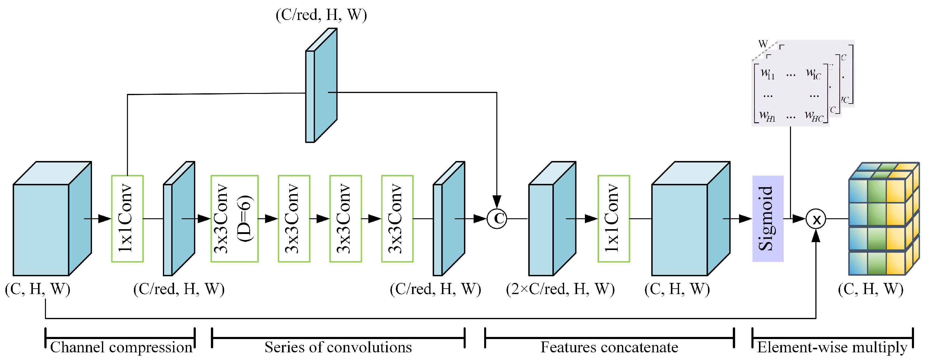
ESA module includes two 1 × 1 convolutional layers, a dilated convolution, a convolutional group of three 3 × 3 convolutional layers, and a sigmoid activation function (Figure 4). It leverages dilated convolutions to extract information across multiple scales while expanding the receptive field. In addition, it utilizes tensor concatenation to preserves low-level and high-level feature representations, capturing more complex patterns and features. Finally, the attention weights assigned to each spatial location are constrained to a bounded range of [0, 1] using a sigmoid activation function. This module is positioned at the beginning of TRAB to improve the pivotal feature representations and allow the model to concentrate on significant spatial regions. And it is positioned at the end for adjusting the weights across spatial locations after the model finishes feature learning, so that important features will be emphasized in the final output, thereby optimizing its overall performance.

RFA module consists of four residual blocks (RBs) and a 1 × 1 convolutional layer as shown in Figure 2b. To effectively integrate multi-level features, the output of the final RB is concatenated with hierarchical features that were derived from the first three RBs. Compared to directly stacked residual blocks, the RFA module facilitates enhanced contextual comprehension of input data, thereby significantly increasing the representational capacity of the learned features. In addition, the RB consists of three 3 × 3 convolutional layers and an ESA module. The three 3 × 3 convolutions enable the model to extract deeper feature representations, and integrating ESA into residual blocks enables adaptive feature region focusing across attention layers, improving feature selection flexibility.

STB consists of two Swin Transformer layers (STLs), which in turn consist of two layer-normalization (LN) layers, a multi-head self-attention (MSA), and a multi-layer perceptron (MLP), as shown in Figure 2c. MSA is used to learn the global and local dependencies of the input features, and the computation of each layer is realized by the local windows, followed by global information integration through a shifted window mechanism. This approach of partitioning the image into shifted windows effectively reduces the token sequence length, constraining self-attention computations to focus solely on features with the window rather than features of the entire image. Consequently, it significantly reduces computational complexity and memory consumption while improving training efficiency. On the other hand, MLP applies nonlinear transformations to attention head outputs for enhanced feature extraction. In summary, it achieves an exemplary balance between representational capacity and computational efficiency, having been extensively validated across numerous visual tasks [48,49,50].

The workflow of TRAB follows a “local focus-global understanding-local refinement” strategy. The first ESA module performs a spatial selection of the input features to achieve localized focusing. The refined features are then processed by the RFA module, which aggregates multi-level local contextual information. Critically, these enriched local features are fed into the STB, which captures long-range dependencies and builds a comprehensive global understanding of the scene. Finally, the second ESA module refines and enhances feature information further, ensuring an optimized final representation.

2.2.3. Loss Function Module

To update model parameters by error back propagation and achieve model convergence through repeated iterations, the loss function calculates the difference between the model output DEM and the InSAR DEM. A masking operation is applied prior to loss computation, restricting it to pixels within non-data missing areas. The total loss function used for model training is composed of three components: a global loss, a SAR feature loss, and a terrain feature loss, which is calculated as follows:

$$L=L_{Global}+L_{SAR}+L_{Terrain}$$

(2)

where $L$ represents the total loss; $L_{Global}$ represents the global loss; $L_{SAR}$ represents SAR feature loss; $L_{Terrain}$ represents terrain feature loss. Among them, the global loss is determined using the formula below:

$$L_{Global}={\displaystyle \frac{1}{n}}{\displaystyle \sum _i^n\left|y_i-\stackrel{\wedge }{y_i}\right|}$$

(3)

where $y_i$ and $\stackrel{\wedge }{y_i}$ separately represent the elevation values of the InSAR DEM and the predicted high-precision DEM; n represents the number of pixels in the InSAR DEM.

SAR feature loss is made up of two components: intensity loss and coherence loss. Since SAR features are used as multi-source data to provide more information for the model to learn elevation, its own value is not directly related to the elevation value. Therefore, the loss of SAR features is calculated by using its value as the weight of the DEM to measure the loss, the formula is as follows:

$$L_{SAR}={\displaystyle \frac{1}{n}}{\displaystyle \sum _i^n{D}_i^{mli}\left|y_i-\stackrel{\wedge }{y_i}\right|}+{\displaystyle \frac{1}{n}}{\displaystyle \sum _i^n{D}_i^{cc}\left|y_i-\stackrel{\wedge }{y_i}\right|}$$

(4)

where $D_i^{mli}$ represents the values of intensity; $D_i^{cc}$ represents the values of coherence.

Terrain feature loss function consists of slope loss and aspect loss combined, which is calculated as follows:

$$L_{Terrain}={\lambda }_1{L}_{Slope}+{\lambda }_2{L}_{Aspect}$$

(5)

$$L_{Slope}={\displaystyle \frac{1}{n}}{\displaystyle \sum _i^n\left|S_i-\stackrel{\wedge }{S_i}\right|}$$

(6)

$$L_{Aspect}={\displaystyle \frac{1}{n}}{\displaystyle \sum _i^n\left|A_i-\stackrel{\wedge }{A_i}\right|}$$

(7)

where $L_{Slope}$ represents the slope loss; $L_{Aspect}$ represents the aspect loss; ${\lambda }_1$ and ${\lambda }_2$ represent the weights of slope and aspect losses, respectively; $S_i$ represents slope values of the InSAR DEM; $\stackrel{\wedge }{S_i}$ represents slope values of the predicted high-precision DEM; $A_i$ represents aspect values of the InSAR DEM; and $\stackrel{\wedge }{A_i}$ represents aspect values of the predicted high-precision DEM. In this case, the formulas for slope and aspect are as follows:

$$Slope=\arctan \sqrt{\Delta {h_x}^2+\Delta {h_y}^2}$$

(8)

$$Aspect=\arctan {\displaystyle \frac{\Delta h_y}{\Delta h_x}}$$

(9)

where $\Delta h_x$ represents the elevation difference between two neighboring pixels of the mage in the east–west direction, while $\Delta h_y$ represents the elevation difference between two neighboring pixels of the mage in the south–north direction.

2.2.4. Accuracy Evaluation

The accuracy of the predicted HR DEM is assessed by the following indicators: the mean absolute error (MAE), root mean square error (RMSE), mean absolute error of slope (${\mathit{MAE}}_{slope}$), and peak signal-to-noise ratio (PSNR). The reconstruction quality is assessed by quantifying the difference between the predicted and actual HR DEMs, and the formulas are as follows:

$$MAE={\displaystyle \frac{1}{n}}{\displaystyle \sum _{i=1}^n\left|y_i-\stackrel{\wedge }{y_i}\right|}$$

(10)

$$RMSE=\sqrt{{\displaystyle \frac{1}{n}}{\displaystyle \sum _{i=1}^n{(y_i-\stackrel{\wedge }{y_i})}^2}}$$

(11)

$$MA{E}_{slope}={\displaystyle \frac{1}{n}}{\displaystyle \sum _{i=1}^n\left|S_i-\stackrel{\wedge }{S_i}\right|}$$

(12)

$$PSNR=10\cdot {\log }_{10}\left({\displaystyle \frac{{y_{\max }}^2}{RMS{E}^2}}\right)$$

(13)

where $y_{\max }$ represents the maximum elevation value in the InSAR DEM.

Based on these indexes, the model’s experimental results are evaluated comparatively with the following typical super-resolution reconstruction models:

• BICUBIC: As a classic interpolation algorithm, it uses a triple interpolation process based on the gray values of the 16 points surrounding the sampling grid.
• SRCNN: It is a classic super-resolution reconstruction model, establishing an end-to-end mapping between low- and high-resolution images through layered convolutional operations.
• EDSR: It mitigates the vanishing gradient problem by eliminating batch normalization layers and optimizing residual learning, significantly expands the network’s training depth.
• RFAN [51]: It is an improvement on residual dense network (RDN), which uses residual feature aggregation framework to integrate informative residual features, thereby producing more representative features.
• HNCT [52]: It combines a convolutional neural network with a Transformer, leveraging their respective capabilities to improve feature extraction and contextual understanding, thereby improving overall performance when processing complex data.

3. Experiments and Results

3.1. Study Area

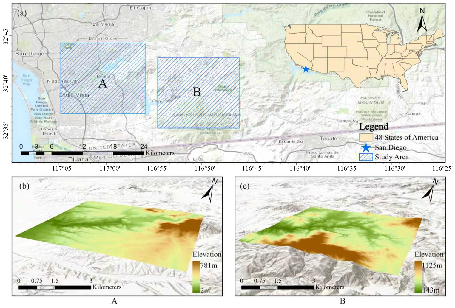
The study areas were two typical regions of San Diego, CA, USA (Figure 5). It is bordered by the Pacific Ocean to the west and mountains to the east. Study areas A (117°5′W~116°56′W, 32°37′N~32°44′N) and B (116°55′W~116°46′W, 32°35′N~32°42′N) cover a wide range of landforms, including coastal plains, hilly mountains, deep river valleys and urbanized areas, with large surface undulations, making them ideal for high-precision DEM reconstruction research.

The origin research data are TerraSAR-X data and ALOS PALSAR DEM, of which a total of 19 scenes of TerraSAR-X data (https://earth.esa.int/eogateway/missions/terrasar-x-and-tandem-x, accessed on 23 January 2024) are used to generate the high-resolution DEM; the 12.5 m resolution ALOS PALSAR DEM (https://search.asf.alaska.edu, accessed on 5 March 2024) functions as low-resolution data for model training.

3.2. Training Details

The sample datasets obtained in Section 2.1 was randomly divided at a ratio of 8:2, allocating 80% (1850 image block pairs) to the training set and 20% (462 image block pairs) to the validation set, and random horizontal and vertical flipping, random scale crop, random rotation were used for data enhancement. All models employed a batch size of 8 and were trained for 1200 epochs utilizing four NVIDIA GeForce GTX 3090 GPUs within the PyTorch 2.2.1 framework. The learning rate was initialized to 1 × 10⁻⁴ and adjusted using the cosine annealing learning rate strategy. The network was optimized using the Adam optimizer (${\beta }_1$ = 0.9, ${\beta }_2$ = 0.999, and $\epsilon$ = 10⁻⁸). And the weights for both slope loss and aspect loss are set to 1 throughout the training process, balancing their comparable importance in terrain representation while enhancing model generalization [42].

3.3. Experiment Results

For evaluating the accuracy of model training, the trained model is used to compare the reconstruction accuracy on the validation set. Higher accuracy indicates more effective training and better capability in addressing the DEM super-resolution reconstruction problem.

Table 1. Comparison of training accuracy of different models.

Model	MAE ↓	RMSE ↓	${\mathit{MAE}}_{\mathit{s}\mathit{l}\mathit{o}\mathit{p}\mathit{e}}$ ↓	PSNR ↑
BICUBIC	3.137095	4.418563	4.173960	37.494330
SRCNN	3.097825	4.420104	4.149862	36.600797
EDSR	2.381658	3.358872	3.729225	38.393006
RFAN	2.298824	3.204749	3.679708	38.670013
HNCT	3.228910	4.584721	4.126889	36.255792
TRAN-ST (Ours)	2.249270	3.160545	3.611090	38.678286

compares training accuracy across several models, and it is evident that compared with the traditional interpolation algorithm and other DEM SR reconstruction models, TRAN-ST is optimal in MAE and RMSE, which represent the elevation accuracy, ${\mathit{MAE}}_{slope}$, which represents the terrain accuracy, and PSNR, which represents the image reconstruction quality. TRAN-ST demonstrates significant improvements across multiple metrics: achieving 2.16–30.34% MAE reduction, 1.38–31.06% RMSE reduction, 1.86–13.48% ${\mathit{MAE}}_{slope}$ reduction, and 0.02–6.68% PSNR improvement compared to baseline models.

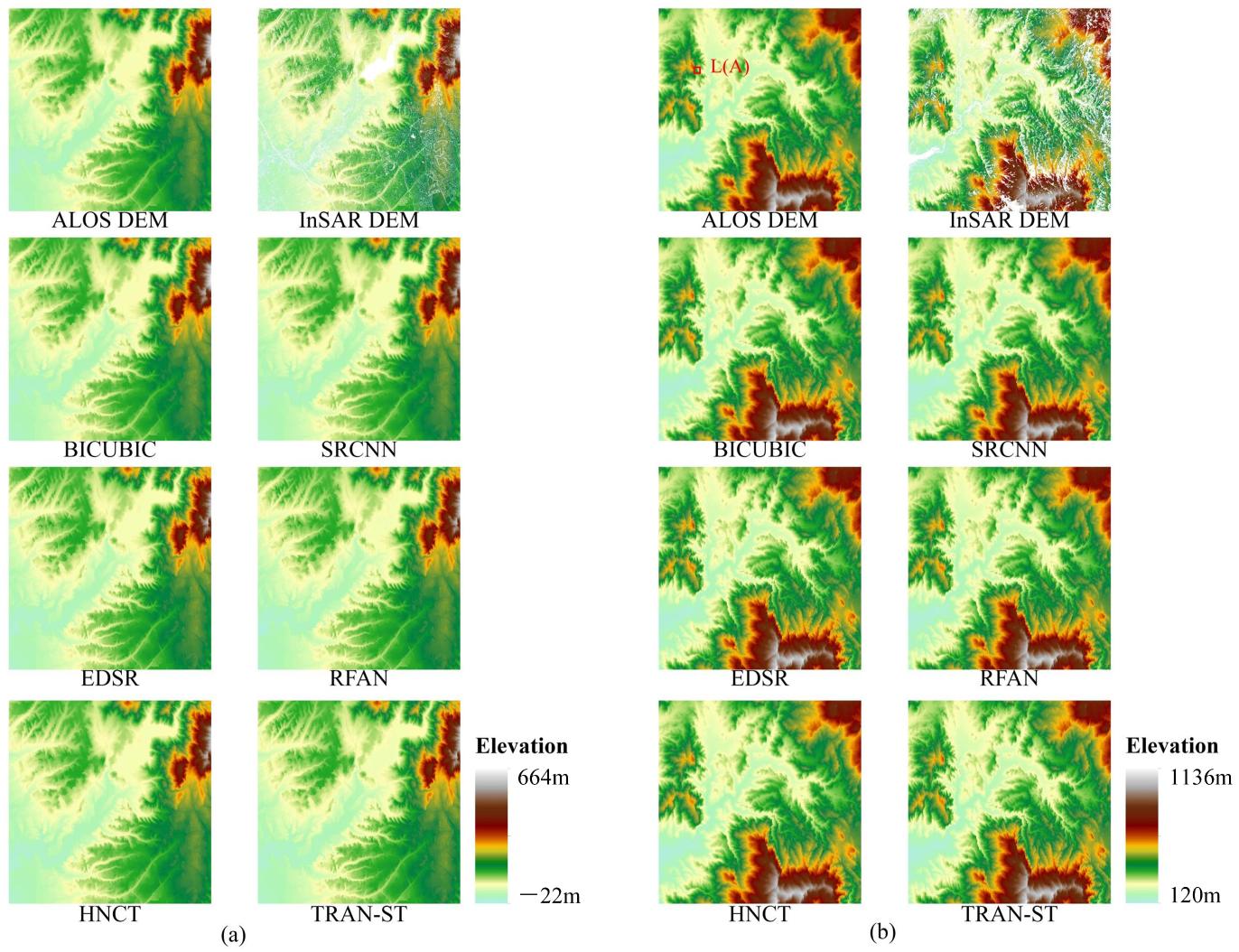
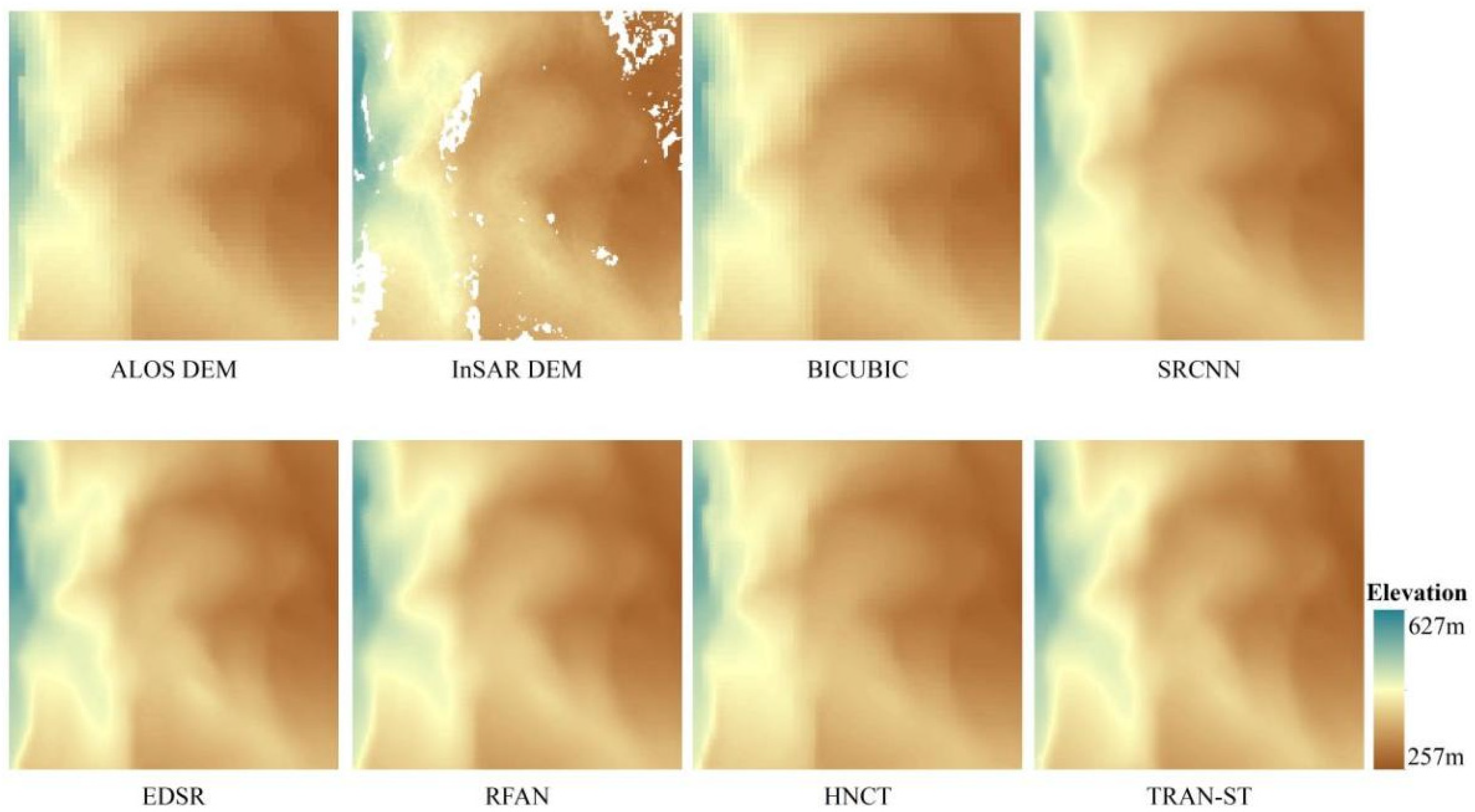
To visualize the accuracy evaluation, the reconstruction of high-resolution DEMs was performed using each trained model separately to obtain the 3 m resolution seamless DEMs. Figure 6 contrasts the model reconstruction results, with Figure 6a and Figure 6b displaying DEM results from study areas A and B, respectively. Each model reconstructs seamless high-resolution DEM, but the specific reconstruction visual effect is not significantly different on a large study area, so the local area L(A) (as shown in Figure 6) is selected for refined comparison. As shown in Figure 7, significant structured grid artifacts were observed in the low-resolution ALOS DEM and its BICUBIC interpolation results. Meanwhile, the reconstruction effect of other models in high relief areas is not smooth, which is manifested by terracing effects and significant structural discrepancies in mountainous areas compared to the InSAR DEM.

While the difference in results between RFAN and TRAN-ST is not significant in overall visualization,

Table 2. Full-pixel statistical metrics of the DEM reconstructed for each model in L(A).

Model	MIN	MAX	MEAN	STD
ALOS DEM	266.73	578.38	372.39	63.75
InSAR DEM	257.48	625.59	380.94	68.43
BICUBIC	267.28	582.99	374.11	65.06
SRCNN	265.89	579.97	372.19	63.81
EDSR	267.92	619.39	381.29	69.95
RFAN	264.38	608.68	381.67	69.04
HNCT	266.01	586.04	371.55	64.16
TRAN-ST (Ours)	265.48	626.28	380.97	68.59

displays quantitative analysis based on the full-pixel statistical metrics, including elevation minima, maxima, means, and standard deviations, revealing differences in statistical distribution characteristics between the two. TRAN-ST shows closer alignment with the InSAR DEM in terms of mean values and standard deviations, demonstrating its statistical superiority in preserving both the central tendency of elevation distributions and spatial heterogeneity within the study area.

The visualization of the global error between models is achieved by calculating the absolute deviation of the full-pixel statistical metrics (Figure 8). The quantitative analysis reveals all models demonstrate inherent limitations in learning minimum elevation values due to the constraints of low-resolution DEM. Although RFAN exhibits a relative advantage with an absolute deviation from the InSAR DEM ($\Delta MIN$ = 6.90 m), its performance shows no statistically significant difference compared to TRAN-ST ($\Delta MIN$ = 8.00 m). In the restoration of maximum elevation values, TRAN-ST shows a statistically superior performance, achieving a 95.92% reduction in deviation from the InSAR DEM ($\Delta MAX$ = 0.69 m) compared to RFAN ($\Delta MAX$ = 16.91 m). The discrepancy with other baseline models is even more pronounced, indicating its improved ability to capture extreme topographic features.

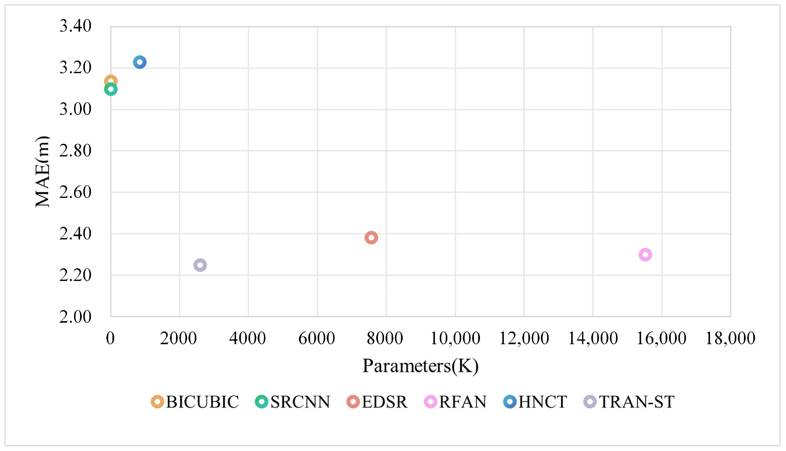
Additionally, to prevent the problem of redundant computational resource consumption caused by indiscriminate expansion of network depth and to explore the balanced relationship between model complexity and reconstruction accuracy, a bivariate scatter plot of parameters-MAE was constructed. It systematically compares the DEM reconstruction performance of different models. The models with lower MAE and fewer parameters have better performance. As shown in Figure 9, TRAN-ST significantly reduces the MAE value compared to BICUBIC, SRCNN, and HNCT, while EDSR and RFAN, although achieving a more similar level of accuracy to TRAN-ST, separately have three and six times more parameters than TRAN-ST, and there is a significant computational redundancy phenomenon. The significant advantage of TRAN-ST with regard to the number of parameters is primarily attributable to the lightweight Transformer module, significantly reducing redundant parameters while maintaining the ability to extract features.

To comprehensively evaluate the engineering applicability of each model, their training efficiency was compared under a unified environment. To ensure a fair comparison, this efficiency analysis employed a controlled variable design: all models utilized the same DEM input and a basic L1 reconstruction loss function. Modules that could introduce additional computational overhead, such as SAR feature integration and terrain feature constraints, were removed to focus solely on assessing the efficiency of the network architecture. As shown in

Table 3. Comparison of training efficiency of different models.

	SRCNN	EDSR	RFAN	HNCT	Our Model
Total training time (hours)	0.81	1.20	8.90	2.23	6.43
Time of each epoch (seconds)	2.45	3.60	26.71	6.69	19.28

, although our proposed model requires longer training times than some other models, this is directly attributable to its deep, complex architectural design choices. Our model employs a deep encoder–decoder structure integrated with multi-scale attention mechanisms. While this intricate design increases the training time per epoch, it endows the model with significantly enhanced feature representation capabilities. Compared to RFAN, which achieves comparable reconstruction accuracy, our model demonstrates a significant efficiency advantage, with training speeds accelerated by approximately 38%. Furthermore, while maintaining competitive reconstruction accuracy, our model exhibits stricter parameter control, reflecting a balanced approach between model complexity and computational efficiency.

4. Discussion

4.1. Enhancing DEM Reconstruction Accuracy with SAR Data

The study area’s 3 m resolution photogrammetric DEM, covering a local target area and downloaded from the United States Department of Agriculture (https://datagateway.nrcs.usda.gov/, accessed on 11 October 2024), was utilized to assess our SAR-integrated model’s performance against other single-source reconstruction models, as shown in Figure 10. This comparison enables a more thorough and comprehensive evaluation of DEM reconstruction results of each model, as the reconstruction accuracy of the missing data area could not be confirmed using InSAR DEM.

As shown in

Table 4. A comparison of accuracy of different models with the photogrammetric DEM.

Model	MAE ↓	RMSE ↓	PSNR ↑
BICUBIC	8.736197	9.701352	34.475817
SRCNN	8.256230	9.264207	34.876297
EDSR	7.804783	9.528105	34.632332
RFAN	6.857835	9.075149	35.055388
HNCT	8.447665	9.434737	34.717866
TRAN-ST (Ours)	6.854576	8.952200	35.173867

, the error between the DEMs obtained from the reconstruction of different models and the photogrammetric DEM is calculated and quantitatively evaluated using the MAE, RMSE and PSNR metrics. It demonstrates that TRAN-ST achieves optimal performance across all three metrics: a 0.04–21.54% reduction in MAE, a 1.35–7.72% improvement in RMSE, and a 0.34–2.02% improvement in PSNR compared to baseline models. Influenced by the elevation error between the InSAR DEMs and photogrammetric DEMs, the accuracy metric values are inferior to the training accuracy values as a whole, but TRAN-ST still shows good reconstruction accuracy through the synergistic optimization of the multi-source feature fusion mechanism and the residual attention module, which also proves its good reconstruction effect in the area of missing DEM values. In summary, compared to SR models based on other single data sources, our SR model incorporating SAR data achieves superior reconstruction results.

To deeply investigate the model’s spatial heterogeneity characteristics, a quantitative assessment of error distribution is conducted between DEMs obtained from several SR reconstruction models and the photogrammetric DEM, with region M(A) in Figure 10 serving as a representative example. The results are shown in Figure 11. The BICUBIC, SRCNN, EDSR, and HNCT models all exhibit significant systematic negative bias, and in comparison, the RFAN and TRAN-ST show closer alignment with the ground truth values in negatively biased pixels. Further quantitative analysis of error distribution across multiple intervals reveals a consistent advantage of TRAN-ST over RFAN. Specifically, within the [−4 m, 4 m] range, TRAN-ST encompasses 88.33% of error pixels, compared to 87.89% for RFAN. More notably, as the interval expands to [−6 m, 6 m], TRAN-ST maintains a higher concentration of errors (97.56% vs. 97.36%), demonstrating that its error distribution is more concentrated and that it produces fewer extreme outliers. Although it produces localized overestimation in the reconstruction of high elevation points, which is considered to be affected by the inherent resolution discrepancies between DEM data and SAR data during the cross-modal feature alignment process, the overall accuracy is still better than other models.

To precisely evaluate the respective contributions of intensity and coherence features in DEM reconstruction, systematic ablation experiments are designed. Specifically, to ensure fairness in evaluation, when removing a specific SAR feature, its corresponding loss function is simultaneously removed. The experimental results (

Table 5. Accuracy metrics for SAR feature ablation experiments.

SAR Feature	Loss Function	MAE ↓	RMSE ↓	${\mathit{MAE}}_{\mathit{s}\mathit{l}\mathit{o}\mathit{p}\mathit{e}}$ ↓	PSNR ↑
/	$L_{Global}+L_{Terrain}$	2.288558	3.223600	3.314659	38.561681
Intensity	$L_{Global}+L_{Terrain}+L_{Intensity}$	2.271661	3.217528	3.611951	38.563072
Coherence	$L_{Global}+L_{Terrain}+L_{Coherence}$	2.263869	3.219768	3.672139	38.606781
Intensity + Coherence	$L_{Global}+L_{Terrain}+L_{SAR}$	2.249270	3.160545	3.611090	38.678286

) indicate that incorporating both intensity and coherence features enhances the elevation accuracy of reconstructed DEMs, yielding improvements in MAE, RMSE and PSNR metrics compared to models without SAR features. It should be noted that the model without SAR features, by learning solely from DEM data, reduces sensitivity to local elevation noise in slope calculations, thereby achieving lower MAE in slope. However, it underperforms on all other metrics compared to other models. Most importantly, the integrated model combining both intensity and coherence features achieved optimal overall performance. Its improvement surpassed the simple sum of the individual contributions from each feature, demonstrating a synergistic enhancement effect between them. This indicates that the effective fusion of these two features enables the model to reconstruct a more accurate DEM.

Having confirmed that fusing SAR data significantly improves reconstruction accuracy, ablation experiments are further conducted to quantify the impact of different SAR features fusion methods. Ablation experiments are compared in terms of the sampling methods used to dimensionally align SAR features with DEMs and the effectiveness of the attentional module used to fuse SAR features, respectively.

SAR features are used as model inputs to learn the InSAR DEM together with the low-resolution DEM. Since there are scale differences between the SAR features and the low-resolution DEM, the shallow features extracted from both need to be dimensionally aligned by sampling prior to feature fusion. Two types of sampling are identified: down-sampling the SAR features (192 × 192) to align them with the low-resolution DEM’s (48 × 48) dimensions, and up-sampling the low-resolution DEM to align it with the SAR features’ dimensions. And three typical interpolation methods—nearest, bilinear, and bicubic—are employed for comparative analysis to evaluate the impact of different up-sampling methods on reconstruction accuracy. As shown in

Table 6. Accuracy metrics for SAR feature fusion method ablation experiments.

Ablation Block	Method		MAE ↓	RMSE ↓	${\mathit{MAE}}_{\mathit{s}\mathit{l}\mathit{o}\mathit{p}\mathit{e}}$ ↓
Sampling method	Down-sample		2.459302	3.644732	3.857245
	Up-sample	Nearest	2.249270	3.160545	3.611090
		Bilinear	2.263302	3.189653	3.624948
		Bicubic	2.320249	3.273505	3.627777
Attention method	/		2.270688	3.177437	3.625823
	CA		2.249270	3.160545	3.611090

, the model using the up-sampling approach substantially outperforms the down-sampling in all metrics due to the fact that the up-sampling can better preserve spatial details and high-frequency information in the original SAR features. Although up-sampling low-resolution DEMs introduces interpolation errors, more plausible spatial distribution patterns can be effectively learned by the subsequent convolutional neural network. Conversely, down-sampling SAR features leads to irreversible loss of critical high-frequency information such as topographic edges and textural characteristics, due to the discard of essential detail data. Additionally, a comparative analysis of interpolation methods for up-sampling shallow features in DEMs was conducted, with results clearly indicating that nearest interpolation is the optimal choice. This is because the objects sampled at this stage are the feature maps extracted from LR DEMs by the convolutional layer. The core objective is to achieve spatial alignment between these feature maps and the shallow feature maps derived from intensity and coherence data rather than introducing additional information or altering the feature distribution. In this process, nearest interpolation effectively avoids feature smoothing and confusion that may arise from bilinear and bicubic interpolation by directly replicating pixel values, thereby maximizing the preservation of the original features’ discriminative power.

Feature fusion is performed on shallow features extracted from the low-resolution DEM and SAR features after dimensional alignment. Ablation experiments, where the CA module is removed from our model, show that CA contributes to improved multi-source feature fusion. By aggregating spatial context through global pooling to generate channel attention weights, CA enables the network to strengthen its response to critical channels of DEM reconstruction while suppressing redundant or conflicting features caused by modal discrepancies.

4.2. Ensuring Topographic Consistency Through Terrain Features

To validate the effectiveness of incorporating terrain features into the model, this study selects slope, aspect, and river network as representative terrain features, and conducts a multi-model comparative analysis of topographic consistency parameters, thereby quantifying the model’s capability in maintaining the spatial distribution of topographic elements.

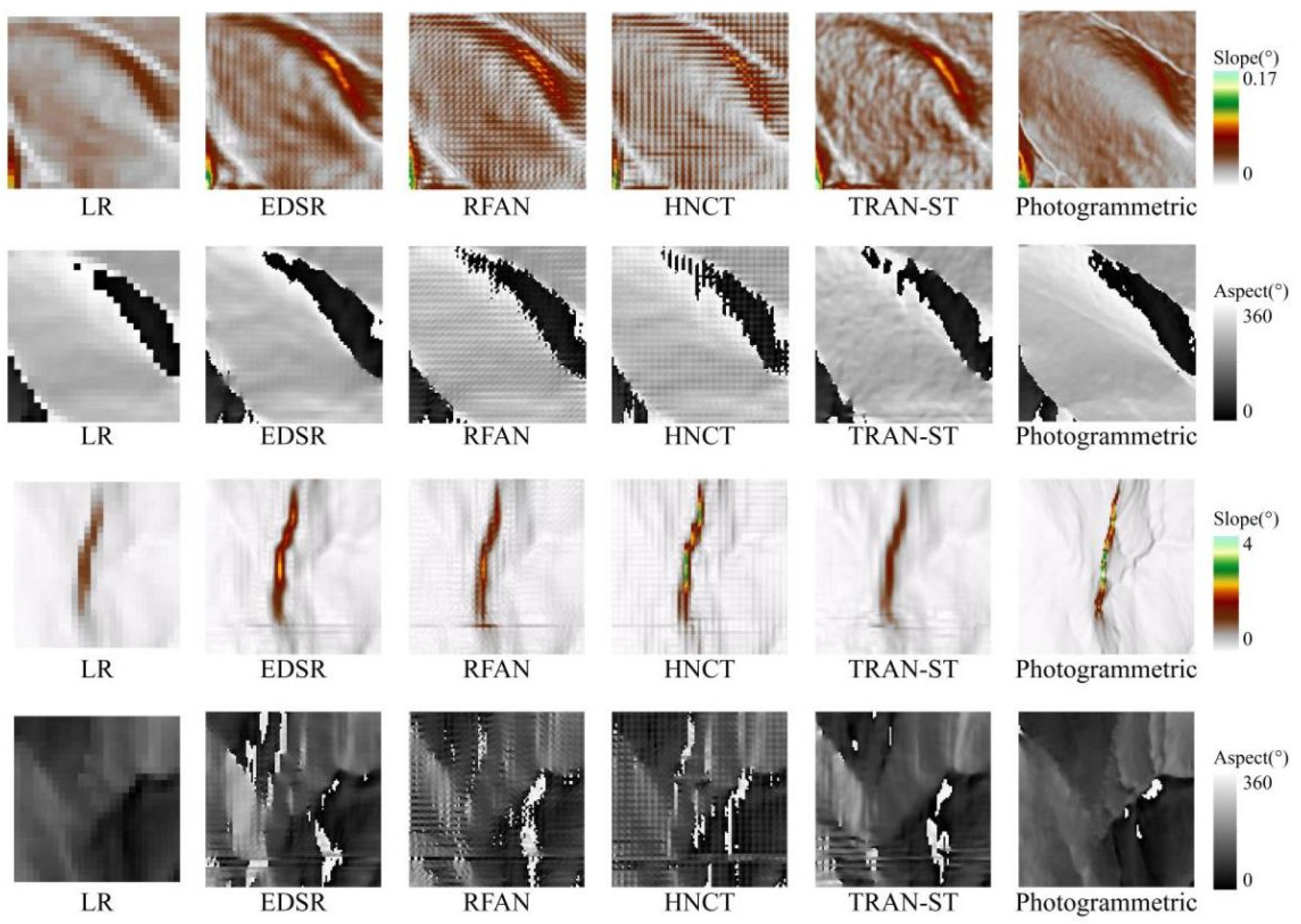
Slope and aspect analyses were conducted for two representative geomorphic study areas, N(A) and N(B), as shown in Figure 10. Study area N(A) is characterized by relatively flat terrain with overall lower elevation values, while N(B) is located in a mountainous area with higher elevation values. A comparative accuracy assessment was performed using MAE and RMSE metrics against the terrain features derived from the photogrammetric DEM. According to the visualization and quantification results in Figure 12 and

Table 7. Accuracy comparison of slope and aspect results from different models with the photogrammetric DEM in N(A) and N(B).

Study Area	Metrics	EDSR	RFAN	HNCT	TRAN-ST
N(A)	${\mathit{MAE}}_{slope}$ ↓	0.008584	0.009013	0.008366	0.007758
	${\mathit{RMSE}}_{slope}$ ↓	0.011644	0.011963	0.011399	0.010913
	${\mathit{MAE}}_{aspect}$ ↓	30.663644	32.056526	33.236173	31.868849
	${\mathit{RMSE}}_{aspect}$ ↓	73.064249	79.406425	80.659781	76.894965
N(B)	${\mathit{MAE}}_{slope}$ ↓	0.158203	0.150141	0.158773	0.136851
	${\mathit{RMSE}}_{slope}$ ↓	0.382609	0.350300	0.403068	0.322392
	${\mathit{MAE}}_{aspect}$ ↓	50.263324	42.811815	38.706966	36.69152
	${\mathit{RMSE}}_{aspect}$ ↓	85.312511	75.109398	69.690326	66.583082

, our model demonstrates closer alignment with the photogrammetric DEM in terms of slope across both gently undulating terrain and high-relief mountainous regions, and the integration of high-precision SAR features enriches texture details of output HR DEM. As for aspect, our model shows superior reconstruction performance in high-relief mountainous areas, while the effect is inferior to EDSR in flat terrain areas. This discrepancy may be due to the fact that the calculation of aspect in flat terrain is more sensitive to minor elevation fluctuations, where critical points of aspect determination have opposite polarities of elevation change. Alternatively, the photogrammetric DEMs may suffer from excessive smoothing, failing to preserve the fine-grained geomorphic details expected from high-resolution DEMs [42]. And the impact on the experimental results caused by the lack of precision in the validation data is also one of the limitations of this study.

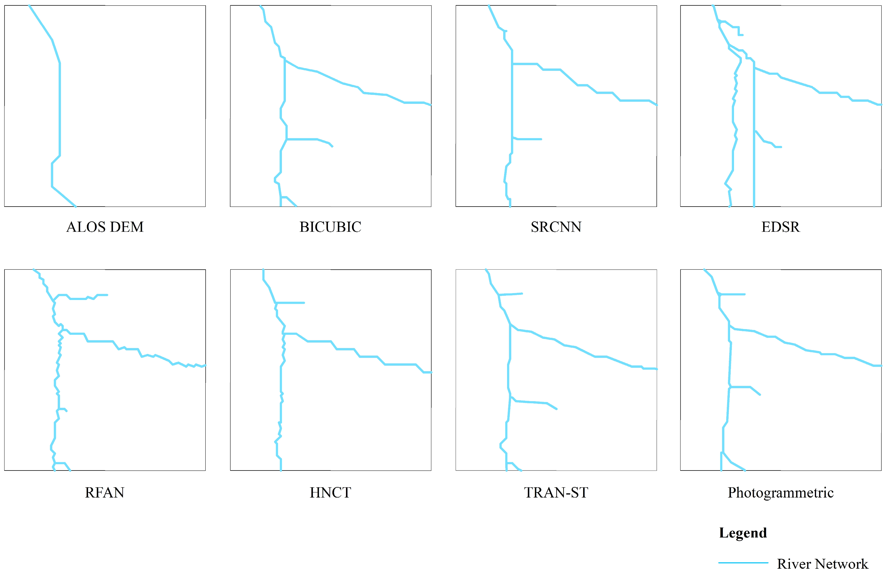
In terms of the river network, the N(C) study area in Figure 10, where the river network is more densely distributed, is selected for comparison of the extraction results. As shown in Figure 13, compared to other models, the river network extracted by TRAN-ST is generally consistent with the photogrammetric DEM. Under unified hydrological extraction standards, TRAN-ST not only accurately reproduces the structure of the main river network but also enables more complete extraction of minor tributaries within the watershed. It confirms that TRAN-ST achieves superior performance in reconstructing hydrologically meaningful terrain structures.

4.3. Network Design for Enhanced Performance

The ablation experiments are compared for the major improvements in TRAB, the core module of this network. One is to validate the ESA blocks in TRAB by replacing all ESA blocks in the module with Spatial Attention (SA) blocks, and the second is to validate the STB by replacing the STB with a 3 × 3 convolutional layer. As shown in

Table 8. Accuracy metrics for TRAB module ablation experiments.

Ablation Block	Method	MAE ↓	RMSE ↓	${\mathit{MAE}}_{\mathit{s}\mathit{l}\mathit{o}\mathit{p}\mathit{e}}$ ↓
Spatial Attention	SA	2.723769	3.861201	3.856078
	ESA	2.249270	3.160545	3.611090
Transformer Block	3 × 3 Conv	2.436377	3.426715	3.783922
	STB	2.249270	3.160545	3.611090

, compared with SA, the ESA block, as an improved spatial attention mechanism, effectively improves the model’s reconstruction accuracy. And STB improves reconstruction effect by improving the global perception ability, and it also substantially reduces the model’s parameters (Figure 9).

Beyond the core module of TRAN-ST, loss function is also crucial to the network architecture by guiding the model optimization process. In order to verify loss function plays a supervisory role in model training, ablation experiments are conducted on the terrain feature loss and SAR feature loss while keeping the training datasets unchanged, and the results are shown in

Table 9. Accuracy metrics for loss function ablation experiments.

Loss Function	MAE ↓	RMSE ↓	${\mathit{MAE}}_{\mathit{s}\mathit{l}\mathit{o}\mathit{p}\mathit{e}}$ ↓	PSNR ↑
$L_{Global}$	2.721057	3.910099	3.940710	37.189309
$L_{Global}+L_{SAR}$	2.295187	3.477773	3.666114	38.561521
$L_{Global}+L_{Terrain}$	2.398073	3.610390	3.334405	37.648377
$L_{Global}+L_{SAR}+L_{Slope}$	2.278481	3.202993	3.589002	38.567027
$L_{Global}+L_{SAR}+L_{Aspect}$	2.254637	3.190442	3.691850	38.645024
$L_{Global}+L_{SAR}+L_{Terrain}$	2.249270	3.160545	3.611090	38.678286

. SAR feature loss includes intensity loss and coherence loss, and terrain feature loss includes slope loss and aspect loss. During the design process of the ablation experiment, considering that SAR data and low-resolution DEM participate together in the DEM SR reconstruction task as multi-source inputs, the two types of data have significant differences in numerical dimensions, which can cause a severe decrease in elevation accuracy if not constrained by SAR feature loss. Therefore, this section does not additionally compare the intensity and coherence losses in the SAR feature loss in separate ablation experiments, and discusses them as a whole. Quantitative results reveal that our model performs optimally on most metrics. Although $L_{Global}+L_{Terrain}$ achieves optimal performance on the ${\mathrm{MAE}}_{slope}$ metric, its MAE and RMSE values are 6.62% and 14.23% higher than those of TRAN-ST, respectively, confirming the critical role of SAR feature loss in improving topographic inversion accuracy. The ablation experiments further demonstrate that the synergistic optimization mechanism of slope and aspect loss effectively facilitates the recovery of terrain detail through joint constraints and improves the overall elevation reconstruction accuracy.

4.4. Limitations and Future Enhancements

While demonstrating competitive performance, the proposed method still possesses several limitations. Firstly, the photogrammetric DEM used for validation lacks sufficient accuracy, restricting our ability to evaluate the sensitivity of SAR features to subtle elevation variations and fine-grained terrain textures. Secondly, current evaluation lacks a systematic analysis of reconstruction error distribution across specific complex terrains like steep slopes, gullies, and urban construction areas. Thirdly, although the model performs well in the selected localized study area, its ability to be generalized across diverse geomorphic types, such as alpine, desert, coastal and highly urbanized terrains, remains unverified.

Future research efforts will explore two main directions to overcome the limitations. Firstly, utilizing high-precision elevation data from LiDAR DEMs or ICESat-2 data would enhance the validation of subtle topographic details, offering more than photogrammetric DEMs can provide. It would enable more accurate quantification of elevation errors and topographic consistency. Secondly, systematic investigation of the model’s performance across different terrain regions should be pursued by constructing datasets featuring detailed topographic annotations, to precisely quantify error patterns and guide future model improvements. Thirdly, extensive experiments involving multi-regional datasets spanning a wider range of geomorphological settings, as well as multi-seasonal remote sensing data, should be conducted to evaluate the model’s transferability.

5. Conclusions

This paper proposes a TRAN-ST algorithm that integrates SAR features and terrain features for DEM super-resolution reconstruction. By jointly using SAR features and DEM data as model inputs and introducing terrain features as part of the loss function, the multi-source feature integration deep learning model demonstrates improved elevation accuracy and enhanced terrain feature preservation capabilities. Meanwhile, the model incorporates a TRAB module that combines the lightweight Transformer with the residual attention mechanism to enable cross-scale modeling of long-range dependencies while maintaining a focus on local detail features for more comprehensive capture of feature information. The experimental results indicate that TRAN-ST provides a significant improvement in elevation and terrain accuracy compared to interpolation and traditional deep learning models used for DEM super-resolution reconstruction. During the model training phase, TRAN-ST improves elevation and terrain accuracy by 30.34% and 13.48%, respectively; when photogrammetric DEM is used for validation, TRAN-ST improves elevation reconstruction accuracy by 21.54%. In addition, the introduction of the lightweight Transformer significantly reduces the model’s parameters, thus saving computational resources. All of the above validate TRAN-ST’s superiority and practical significance in DEM super-resolution reconstruction research.

However, this study still has some limitations: First, the photogrammetric DEM used in the current validation process lacks sufficient accuracy, making it difficult to fully verify the sensitivity of the SAR data to subtle elevation changes. Future studies should include LiDAR DEMs or ICESat-2 data to perform cross-validation for terrain texture details beyond the capabilities of the photogrammetric DEM. Second, this study lacks a systematic analysis of reconstruction errors in specific complex terrains, and future work should construct datasets annotated with terrain categories to comprehensively understand the model’s performance boundaries. Third, although the method demonstrates efficient terrain reconstruction capability in the local study area, its generalizability to a wide range of complex geomorphological scenarios still needs to be further verified by multi-regional and multi-seasonal remote sensing data, which provides a key algorithmic validation of the technical path of reconstructing high-resolution DEM based on the synergy of multi-source data.

References

1. Sharma, A.; Tiwari, K.N. A comparative appraisal of hydrological behavior of SRTM DEM at catchment level. J. Hydrol. 2014, 519, 1394–1404. [Google Scholar] [CrossRef]
2. Zhang, Z.; Li, J.; Chen, S.; Liu, Y. Spatial distribution of affordable houses in cities: A case study of Wuhan based on DEM. Acta Geogr. Sin. 2011, 66, 1309–1320. [Google Scholar]
3. Xiong, L.; Li, S.; Hu, G.; Wang, K.; Chen, M.; Zhu, A.; Tang, G. Past rainfall-driven erosion on the Chinese loess plateau inferred from archaeological evidence from Wucheng City, Shanxi. Commun. Earth Environ. 2023, 4, 4. [Google Scholar] [CrossRef]
4. Yamazaki, D.; Ikeshima, D.; Tawatari, R.; Yamaguchi, T.; O’Loughlin, F.; Neal, J.C.; Sampson, C.C.; Kanae, S.; Bates, P.D. A high-accuracy map of global terrain elevations. Geophys. Res. Lett. 2017, 44, 5844–5853. [Google Scholar] [CrossRef]
5. Islam, M.T.; Meng, Q. An exploratory study of Sentinel-1 SAR for rapid urban flood mapping on Google Earth Engine. Int. J. Appl. Earth Obs. Geoinf. 2022, 113, 103002. [Google Scholar] [CrossRef]
6. Demirkesen, A.C.; Evrendilek, F. Digital terrain characterization and interpretation of Lake Van region for earthquake vulnerability combining remote sensing and geographical information systems. Fresenius Environ. Bull. 2017, 26, 1745–1755. [Google Scholar]
7. Zhou, C.; Gan, L.; Cao, Y.; Wang, Y.; Segoni, S.; Shi, X.; Motagh, M.; Singh, R.P. Landslide susceptibility assessment of the Wanzhou district: Merging landslide susceptibility modelling (LSM) with InSAR-derived ground deformation map. Int. J. Appl. Earth Obs. Geoinf. 2025, 136, 104365. [Google Scholar] [CrossRef]
8. Liu, X. Airborne LiDAR for DEM generation: Some critical issues. Prog. Phys. Geogr. 2008, 32, 31–49. [Google Scholar] [CrossRef]
9. Rabiu, L.; Ahmad, A. Unmanned aerial vehicle photogrammetric products accuracy assessment: A review. Int. Arch. Photogramm. Remote Sens. Spat. Inf. 2023, 48, 279–288. [Google Scholar] [CrossRef]
10. Toutin, T.; Gray, L. State-of-the-art of elevation extraction from satellite SAR data. ISPRS J. Photogramm. Remote Sens. 2000, 55, 13–33. [Google Scholar] [CrossRef]
11. Yang, C.; Zhao, F.; Wang, C.; Wang, M.; Liu, X.; Wang, R. A novel topography retrieval algorithm based on single-pass polarimetric SAR data and terrain dependent error analysis. Remote Sens. 2022, 14, 3176. [Google Scholar] [CrossRef]
12. Jiang, H.; Zhang, L.; Wang, Y.; Liao, M. Fusion of high-resolution DEMs derived from COSMO-SkyMed and TerraSAR-X InSAR datasets. J. Geod. 2014, 88, 587–599. [Google Scholar] [CrossRef]
13. Lepcha, D.C.; Goyal, B.; Dogra, A.; Goyal, V. Image super-resolution: A comprehensive review, recent trends, challenges and applications. Inf. Fusion 2023, 91, 230–260. [Google Scholar] [CrossRef]
14. Wang, P.; Bayram, B.; Sertel, E. A comprehensive review on deep learning based remote sensing image super-resolution methods. Earth-Sci. Rev. 2022, 232, 104110. [Google Scholar] [CrossRef]
15. Achilleos, G.A. The inverse distance weighted interpolation method and error propagation mechanism—Creating a DEM from an analogue topographical map. J. Spat. Sci. 2011, 56, 283–304. [Google Scholar] [CrossRef]
16. Fahmy, G. Single image super resolution using E-SPLINE functions. In Proceedings of the 2015 IEEE International Symposium on Signal Processing and Information Technology (ISSPIT), Abu Dhabi, United Arab Emirates, 7–10 December 2015; pp. 623–628. [Google Scholar]
17. Chung, M.; Jung, M.; Kim, Y. Enhancing remote sensing image super-resolution guided by bicubic-downsampled low-resolution image. Remote Sens. 2023, 15, 3309. [Google Scholar] [CrossRef]
18. Chaplot, V.; Darboux, F.; Bourennane, H.; Leguedois, S.; Silvera, N.; Phachomphon, K. Accuracy of interpolation techniques for the derivation of digital elevation models in relation to landform types and data density. Geomorphology 2006, 77, 126–141. [Google Scholar] [CrossRef]
19. Wang, L.; Xiang, S.; Meng, G.; Wu, H.; Pan, C. Edge-directed single-image super-resolution via adaptive gradient magnitude self-interpolation. IEEE Trans. Circuits Syst. Video Technol. 2013, 23, 1289–1299. [Google Scholar] [CrossRef]
20. Zhang, K.; Gao, X.; Tao, D.; Li, X. Single image super-resolution with non-local means and steering kernel regression. IEEE Trans. Image Process. 2012, 21, 4544–4556. [Google Scholar] [CrossRef]
21. Khattab, M.M.; Zeki, A.M.; Alwan, A.A.; Badawy, A.S. Regularization-based multi-frame super-resolution: A systematic review. J. King Saud Univ. Comput. Inf. Sci. 2020, 32, 755–762. [Google Scholar] [CrossRef]
22. Chua, K.K.; Tay, Y.H. Enhanced image super-resolution technique using convolutional neural network. In Proceedings of the 3rd International Visual Informatics Conference (IVIC), Selangor, Malaysia, 13–15 November 2013; pp. 157–164. [Google Scholar]
23. Dong, C.; Loy, C.C.; He, K.; Tang, X. Learning a deep convolutional network for image super-resolution. In Proceedings of the ECCV: 13th European Conference, Zurich, Switzerland, 6–12 September 2014; pp. 184–199. [Google Scholar]
24. Kim, J.; Lee, J.K.; Lee, K.M. Accurate image super-resolution using very deep convolutional networks. In Proceedings of the 2016 IEEE Conference on Computer Vision and Pattern Recognition (CVPR), Las Vegas, NV, USA, 27–30 June 2016; pp. 1646–1654. [Google Scholar]
25. Shi, W.Z.; Caballero, J.; Huszár, F.; Totz, J.; Aitken, A.P.; Bishop, R.; Rueckert, D.; Wang, Z.H. Real-time single image and video super-resolution using an efficient sub-pixel convolutional neural network. In Proceedings of the 2016 IEEE Conference on Computer Vision and Pattern Recognition (CVPR), Las Vegas, NV, USA, 27–30 June 2016; pp. 1874–1883. [Google Scholar]
26. Lim, B.; Son, S.; Kim, H.; Nah, S.; Lee, K.M. Enhanced deep residual networks for single image super-resolution. In Proceedings of the 2017 IEEE Conference on Computer Vision and Pattern Recognition Workshops (CVPRW), Honolulu, HI, USA, 21–26 July 2017; pp. 1132–1140. [Google Scholar]
27. Zhang, Y.; Tian, Y.; Kong, Y.; Zhong, B.; Fu, Y. Residual dense network for image super-resolution. In Proceedings of the 2018 IEEE Conference on Computer Vision and Pattern Recognition (CVPR), Salt Lake City, UT, USA, 18–23 June 2018; pp. 2472–2481. [Google Scholar]
28. Goodfellow, I.; Pouget-Abadie, J.; Mirza, M.; Xu, B.; Warde-Farley, D.; Ozair, S.; Courville, A.; Bengio, Y. Generative adversarial networks. Commun. ACM 2020, 63, 139–144. [Google Scholar] [CrossRef]
29. Ledig, C.; Theis, L.; Huszar, F.; Caballero, J.; Cunningham, A.; Acosta, A.; Aitken, A.; Tejani, A.; Totz, J.; Wang, Z.; et al. Photo-realistic single image super resolution using a generative adversarial network. In Proceedings of the 2017 IEEE Conference on Computer Vision and Pattern Recognition (CVPR), Honolulu, HI, USA, 21–26 July 2017; pp. 105–114. [Google Scholar]
30. Wang, X.; Yu, K.; Wu, S.; Gu, J.; Liu, Y.; Dong, C.; Qiao, Y.; Loy, C.C. ESRGAN: Enhanced super-resolution generative adversarial networks. In Proceedings of the Computer Vision—ECCV 2018 Workshops, Munich, Germany, 8–14 September 2018; pp. 63–79. [Google Scholar]
31. Xu, Z.; Chen, Z.; Yi, W.; Gui, Q.; Hou, W.; Ding, M. Deep gradient prior network for DEM super-resolution: Transfer learning from image to DEM. ISPRS J. Photogramm. Remote Sens. 2019, 150, 80–90. [Google Scholar] [CrossRef]
32. Deng, X.; Hua, W.; Liu, X.; Chen, S.; Zhang, W.; Duan, J. D-SRCAGAN: DEM super-resolution generative adversarial network. IEEE Geosci. Remote Sens. Lett. 2022. [Google Scholar] [CrossRef]
33. Zhang, Y.; Yu, W. Comparison of DEM super-resolution methods based on interpolation and neural networks. Sensors 2022, 22, 745. [Google Scholar] [CrossRef]
34. Zhou, A.; Chen, Y.; Wilson, J.P.; Su, H.; Xiong, Z.; Cheng, Q. An enhanced double-filter deep residual neural network for generating super resolution DEMs. Remote Sens. 2021, 13, 3089. [Google Scholar] [CrossRef]
35. Jiang, Y.; Xiong, L.; Huang, X.; Li, S.; Shen, W. Super-resolution for terrain modeling using deep learning in high mountain Asia. Int. J. Appl. Earth Obs. Geoinf. 2023, 118, 103296. [Google Scholar] [CrossRef]
36. Gao, B.; Yue, L. DEM super-resolution assisted by remote sensing images content feature. In Proceedings of the 5th International Conference on Geology, Mapping and Remote Sensing (ICGMRS), Wuhan, China, 12–14 April 2024; pp. 122–126. [Google Scholar]
37. Vaswani, A.; Shazeer, N.; Parmar, N.; Uszkoreit, J.; Jones, L.; Gomez, A.N.; Kaiser, L.; Polosukhin, I. Attention is all you need. In Proceedings of the 31st International Conference on Neural Information Processing Systems, Long Beach, CA, USA, 4–9 December 2017; pp. 6000–6010. [Google Scholar]
38. Wang, S.; Li, B.Z.; Khabsa, M.; Fang, H.; Ma, H. Linformer: Self-attention with Linear Complexity. arXiv 2020. [Google Scholar] [CrossRef]
39. Choromanski, K.; Likhosherstov, V.; Dohan, D.; Song, X.; Gane, A.; Sarlos, T.; Hawkins, P.; Davis, J.; Mohiuddin, A.; Kaiser, L.; et al. Rethinking Attention with Performers. arXiv 2022. [Google Scholar] [CrossRef]
40. Yang, F.; Yang, H.; Fu, J.; Lu, H.; Guo, B. Learning texture transformer network for image super-resolution. In Proceedings of the 2020 IEEE Conference on Computer Vision and Pattern Recognition (CVPR), Seattle, WA, USA, 13–19 June 2020; pp. 5790–5799. [Google Scholar]
41. Liu, Z.; Zhou, D.; Liu, Y. Image super-resolution network based on global dependency Transformer. J. Comput. Appl. 2024, 44, 1588–1596. [Google Scholar]
42. Zhang, T.; Chen, Y.; Zhu, R.; Wilson, J.P.; Song, J.; Chen, R.; Liu, L.; Bao, L. An intelligent learning reconfiguration model based on optimized transformer and multisource features (TMSFs) for high-precision InSAR DEM void filling. IEEE Trans. Geosci. Remote Sens. 2025, 63, 5203418. [Google Scholar] [CrossRef]
43. Zhang, W.; Zhu, W.; Tian, X.; Zhang, Q.; Zhao, C.; Niu, Y.; Wang, C. Improved DEM reconstruction method based on multibaseline InSAR. IEEE Geosci. Remote Sens. Lett. 2022, 19, 4011505. [Google Scholar] [CrossRef]
44. Zhang, T.; Chen, Y.; Zhang, L.; Wilson, J.P.; Zhu, R.; Chen, R.; Li, Z. Multibaseline interferometry based on independent component analysis and InSAR combinatorial modeling for high-precision DEM reconstruction. IEEE Trans. Geosci. Remote Sens. 2025, 63, 5205417. [Google Scholar] [CrossRef]
45. Liu, Y.; Qian, J.; Wang, L.; Wang, Y. Elevation reconstruction combining SAR intensity and interferometric phase data. In Proceedings of the IGARSS 2022—2022 IEEE International Geoscience and Remote Sensing Symposium, Kuala Lumpur, Malaysia, 17–22 July 2022; pp. 1107–1110. [Google Scholar]
46. Wang, S.; Zhang, G.; Chen, Z.; Cui, H.; Zheng, Y.; Xu, Z.; Li, Q. Surface deformation extraction from small baseline subset synthetic aperture radar interferometry (SBAS-InSAR) using coherence-optimized baseline combinations. GISci. Remote Sens. 2022, 59, 295–309. [Google Scholar] [CrossRef]
47. Hu, J.; Shen, L.; Sun, G. Squeeze-and-excitation networks. In Proceedings of the 2018 IEEE Conference on Computer Vision and Pattern Recognition (CVPR), Salt Lake City, UT, USA, 18–23 June 2018; pp. 7132–7141. [Google Scholar]
48. Wang, L.; Li, R.; Zhang, C.; Fang, S.; Duan, C.; Meng, X.; Atkinson, P.M. UNetFormer: A UNet-like transformer for efficient semantic segmentation of remote sensing urban scene imagery. ISPRS J. Photogramm. Remote Sens. 2022, 190, 196–214. [Google Scholar] [CrossRef]
49. Xu, Z.; Zhang, W.; Zhang, T.; Yang, Z.; Li, J. Efficient Transformer for Remote Sensing Image Segmentation. Remote Sens. 2021, 13, 3585. [Google Scholar] [CrossRef]
50. Xiao, X.; Zhang, Y.; Wang, W.; Wang, C.; Jin, X.; Jin, Y. A lightweight fire detection method based on improved Swin-Transformer. In Proceedings of the 39th Youth Academic Annual Conference of Chinese-Association-of-Automation (YAC), Dalian, China, 7–9 June 2024; pp. 1550–1555. [Google Scholar]
51. Liu, J.; Zhang, W.; Tang, Y.; Tang, J.; Wu, G. Residual feature aggregation network for image super-resolution. In Proceedings of the 2020 IEEE Conference on Computer Vision and Pattern Recognition (CVPR), Seattle, WA, USA, 13–19 June 2020; pp. 2356–2365. [Google Scholar]
52. Fang, J.; Lin, H.; Chen, X.; Zeng, K. A hybrid network of CNN and transformer for lightweight image super-resolution. In Proceedings of the 2020 IEEE Conference on Computer Vision and Pattern Recognitio. Workshops (CVPRW), New Orleans, LA, USA, 18–24 June 2022; pp. 1102–1111. [Google Scholar]
Figure 1. A workflow of the proposed DEM super-resolution reconstruction method.
Remotesensing 17 03625 g001
Figure 2. The structure of the Transformer-based residual attention network (TRAN-ST).
Remotesensing 17 03625 g002
Figure 3. Structure of channel attention (CA).
Remotesensing 17 03625 g003
Figure 4. Structure of enhanced spatial attention (ESA).
Remotesensing 17 03625 g004
Figure 5. An overview of the study area. (a) The location distribution of study area A and study area B. (b) The elevation distribution of study area A. (c) The elevation distribution of study area B.
Remotesensing 17 03625 g005
Figure 6. A comparison of DEM reconstruction results of the study area based on each model. (a) The comparison of DEM reconstruction results in study area A. (b) The comparison of DEM reconstruction results in study area B.
Remotesensing 17 03625 g006
Figure 7. Comparison of DEM local area reconstruction results on each model in L(A).
Remotesensing 17 03625 g007
Figure 8. Global error of each model based on full-cell statistical metrics in L(A).
Remotesensing 17 03625 g008
Figure 9. Comparison of reconstruction performance on each model.
Remotesensing 17 03625 g009
Figure 10. A comparison of reconstruction results of the photogrammetric DEM validation area.
Remotesensing 17 03625 g010
Figure 11. The DEM error distribution between different models and photogrammetry in M(A).
Remotesensing 17 03625 g011
Figure 12. Comparison of slope and aspect results for different models in N(A) and N(B).
Remotesensing 17 03625 g012
Figure 13. Comparison of river network results for different models in N(C).
Remotesensing 17 03625 g013