Machine Learning-Based Sea Surface Wind Speed Retrieval from Dual-Polarized Sentinel-1 SAR During Tropical Cyclones

Highlights

What are the main findings?

• Machine learning models for TC wind speed retrieval are proposed using dual-polarized S-1 SAR data after noise removal, which can reduce the impact of additive and multiplicative noise on cross-polarized data.
• The variable of SST was introduced in the proposed machine learning model for C-band SAR data and improved wind speed inversion results under TC conditions.

What are the implications of the main findings?

• The approach of fusing advanced signal processing (noise removal) with machine learning models that incorporate relevant geophysical variables can be extended to other satellite sensors and to retrieving other oceanic or atmospheric parameters.
• SST is a critical physical variable in the TC wind retrieval process that has been previously underutilized or overlooked in C-band SAR models.

Abstract

Spaceborne Synthetic Aperture Radar (SAR) can be applied for monitoring tropical cyclones (TCs), but co-polarized C-band SAR suffers from signal saturation such that it is improper for high wind-speed conditions. In contrast, cross-polarized SAR data does not suffer from this issue, but the retrieval algorithm needs more deliberation. Previously, many geophysical model functions (GMFs) have been developed using cross-polarized data, which obtain wind speeds using the complex relationships described by radar backscatter, incidence angle, wind direction, and radar look direction. In this regard, the rapid development of artificial intelligence technology has provided versatile machine learning methods for such a nonlinear inversion problem. In this study, we comprehensively compare the wind-speed retrieval performance of several models including Back Propagation Neural Network (BPNN), Support Vector Machine (SVM), Random Forest (RF), and Deep Neural Network (DNN), which were developed based on spatio-temporal matching and correlation analysis of stepped frequency microwave radiometer (SFMR) and dual-polarized Sentinel-1 SAR data after noise removal. A data set with ~2800 samples is generated during TCs for training and validating the inversion model. The generalization ability of different models is tested by the reserved independent data. When using similar parameters with GMFs, RF inversion has the highest accuracy with a Root Mean Square Error (RMSE) of 3.40 m/s and correlation coefficient of 0.94. Furthermore, considering that the sea surface temperature is a crucial factor for generating TCs and influencing ocean backscattering, its effects on the proposed RF model are also explored, the results of which show improved wind-speed retrieval performances.

1. Introduction

Tropical cyclones (TCs) are large storm systems that are usually accompanied by strong winds, large storm surges, flash floods, and other natural disasters, and can be a serious threat to the lives and safety of property of coastal residents [1]. The number of people experiencing risks associated with TCs has steadily increased over the past two decades [2]. Accordingly, timely and accurate monitoring of the intensity and movement of TCs has become very important for coastal countries to protect the safety of their citizens. In addition, the sea surface wind field is also one of the most important parameters for coastal countries to study in oceanography and meteorology [3].

Traditional means to obtain the sea surface wind field include weather stations on land and islands, buoys, or reports from ships on long voyages [4]. These methods have the disadvantages of being affected by weather and limited discontinuous measurement areas and cannot meet the needs of research on and application to TCs [5]. Optical sensors and light detection and ranging (LiDAR) sensors are important instruments for ocean applications but cannot penetrate the thick clouds that are characteristic of TCs, making them fundamentally unsuitable for observing the sea surface beneath these cyclones. Radar altimeters can provide the along-track sea surface wind speed (SSW), which is measured at a height of 10 m above the sea surface, but are limited in spatial coverage. Therefore, spaceborne microwave scatterometers, radiometers, and synthetic aperture radar (SAR) have become common tools to obtain sea surface wind field information over large spatial scales under all-time and all-weather conditions [6]. However, the coarse spatial resolution of scatterometers and radiometers, typically on the order of about 10 km, limits their ability to resolve fine scale wind gradient variations between a TC’s eye and eyewall. In contrast, SAR stands out as a uniquely effective tool for estimating SSWs and characterizing the inner-core structure of TCs with resolutions as high as 1 km. Among SAR satellites, Radarsat-2 and Sentinel-1 (S-1) have been widely used due to the suitability of C-band compared to other frequencies. To retrieve reliable SSW, various empirical geophysical model functions (GMFs) [7,8,9,10] and polarization ratio (PR) models [11,12] have been established by previous researchers based on radar backscatter, incidence angle, wind direction, and other related parameters of co-polarized (VV or HH) data from C-band scatterometers and SAR, which can show high precision for moderate and low sea surfaces. However, the signal saturation phenomenon of co-polarized data occurs when SSW exceeds 33 m/s, thereby resulting in large inversion errors [13].

Compared with GMFs based on co-polarized data, GMFs such as C-2PO [14], H14 [15], C-3PO [16], and QPS-CP [17], established for cross-polarized (VH and HV polarization) data, have addressed the lack of C-band SAR in high-SSW inversion. These GMFs can be used to retrieve SSWs larger than 70 m/s [18]. However, there are certain problems in retrieving low SSW [19] using cross-polarized SAR data because they can be influenced by thermal noise and the scalloping effect [20,21]. Some researchers adopted piecewise equations in the SSW inversion of TCs [1,22] by using co-polarized models for medium and low SSWs and cross-polarized models for high SSWs due to the wide SSW range under TC conditions. In addition, it was found that the model based on co-polarized SAR data and variational methods can take error factors into account and obtain more accurate wind field information under medium and low SSW conditions compared with single-polarized GMFs [23,24]. Therefore, Mouche et al. [25,26] proposed the MS1A model based on C-band dual-polarized SAR data and a two-dimensional variational approach, which can be used to retrieve extreme SSWs up to 80 m/s. Gao et al. [27] tried to use the multiple linear regression (MLR) regression analysis method to retrieve TC wind speeds. However, these models based on traditional empirical or statistical methods may not solve the above nonlinear inversion problems well considering the complex correlation between dual-polarized data and SSWs.

With the rapid development of machine learning technology and massive accumulation of remote sensing data, research based on artificial intelligence (AI) methods has gradually become one of the hot directions in the field of geoscience and can help to improve the accuracy of related remote sensing retrievals [28]. In recent years, scientists have used machine learning methods to solve nonlinear problems of SSW retrieval, which has confirmed their great potential. Horstmann et al. [29] developed a neural network model for retrieving SSW by establishing a data set at a global scale based on ERS-2 SAR data and collocated SSWs from an ERS-2 SCAT scatterometer and ECMWF model. Qin et al. [30] developed an SSW inversion model based on a back propagation neural network (BPNN) for HH-polarized SAR images. This method was more suitable than conventional methods for wind field monitoring in the Arctic region. Mu et al. [31] established a deep learning model to invert the SSWs. Their model integrated the basic idea of residual networks and used different types of input parameters such as physical, texture, and geographic features. In our previous work, a co-polarized scheme was developed with a neural network method, yielding a better performance than conventional CMOD models [32]. A more recent study applied three machine learning algorithms (XGBoost, Multi-layer Perceptron, and K-Nearest Neighbor) to obtain TC wind speeds using S-1 SAR data [33].

Up to now, the retrieval of SSW using machine learning methods has been well applied, but there is a lack of comparative research among machine learning and deep learning algorithms for dual-polarized SAR remote sensing data under high SSW conditions. In this context, this study aims to shine a light on this research area. The correlation between different conventional GMFs model parameters and SSW is analyzed using the method of Pearson correlation analysis through the spatio-temporal matching data of stepped frequency microwave radiometer (SFMR) and S-1 dual-polarized data from 25 SAR images during TCs. And the optimal model parameter combination is determined by comparisons between RF models with different inputting parameters. Four SSW inversion models based on different machine learning and deep learning methods including BPNN, RF, Support Vector Machine (SVM), and Deep Neural Network (DNN) are then established and compared.

Moreover, it is well known that the sea surface temperature (SST) is an essential factor for generating TCs [34]. In addition, the SST signature of thermal fronts and eddies could be discernible by SAR images under nonneutral atmospheric conditions [35,36]. With developments in radar imaging theories and techniques, the effects of SST on radar backscattering and SSW retrievals have been further studied. Liu et al. [37] interpreted the generation of low normalized radar crossing section (NRCS) in SAR images to be related to the thermal front of the Gulf Stream. Under neutral conditions, SST can also impact on the wind retrieval at the C-band radar by viscous damping of short waves [38] and modulating air density and seawater viscosity [39]. Currently, a Ku-band GMF, which takes SST into consideration, has been developed for RapidScat to better retrieve SSWs [40]. But it has not been introduced in C-band models to invert TC winds by previous related studies. Therefore, the influence of SST on inversion results based on dual-polarized SAR data should be explored. The main contributions of this study are summarized as follows:

(1)

Machine learning models for TC wind speed retrieval are proposed using dual-polarized S-1 SAR data after noise removal to reduce the impact of additive and multiplicative noise on cross-polarized data.

(2)

Different SSW model results during TCs based on traditional GMFs (CMOD5.N and S1IW.NR) and machine learning methods (BPNN, RF, SVM, and DNN) are compared, whose results show that the RF model has a better performance.

(3)

The variable of SST was introduced in the proposed RF model, which can improve SSW inversion results under high wind conditions.

This article is organized as follows. Section 2 briefly describes the data used in this study. Section 3 mainly introduces the SSW retrieval model based on traditional GMFs and machine learning methods. Section 4 shows the inversion results obtained by different models on the training, validation, and test sets. The selection of model parameters is also examined using correlation analysis and comparative experiments. Discussion and conclusions are given in Section 5 and Section 6.

2. Datasets

2.1. Data Sets

2.1.1. S-1 SAR Data

The S-1 SAR mission, operated by the European Space Agency, consists of two satellites, S1A and S1B, which were launched in 2014 and 2016, respectively. These two satellites are equipped with C-band SAR sensors with a center frequency of 5.405 GHz and four imaging modes: stripmap (SM), wave (WV), Interferometric Wide (IW), and Extra Wide (EW) modes. Among them, the IW and EW modes can provide a width of ~250 km and 410 km, which can be suitable for the inversion of large-scale TC wind speed. A total of 25 scenes of S-1 SAR images during TCs were collected with incidence angles ranging from 29° to 47° and polarizations of VV and VH. The detailed information of the SAR images is shown in

Table 1. Parameters of S1 SAR images during tropical cyclones.

TC Name	Time	Satellites	Mode	Number
Darby	22 July 2016 15:59	S1A	IW	1
Darby	23 July 2016 04:30	S1A	IW	1
Franklin	9 August 2017 12:01	S1A	IW	1
Florence	13 September 2018 23:12	S1B	IW	1
Florence	14 September 2018 11:15	S1B	IW	1
Micheal	8 October 2018 23:50	S1B	EW	1
Dorian	27 August 2019 22:19	S1A	IW	1
Dorian	29 August 2019 10:21	S1B	IW	1
Dorian	30 August 2019 22:46	S1A	IW	1
Dorian	31 August 2019 10:53	S1A	IW	2
Dorian	3 September 2019 11:17	S1A	IW	2
Dorian	4 September 2019 11:07	S1B	IW	2
Dorian	13 September 2019 11:08	S1B	IW	2
Isais	2 August 2020 23:20	S1B	IW	1
Delta	8 October 2020 00:07	S1B	IW	1
Delta	8 October 2020 00:08	S1B	IW	1
Delta	9 October 2020 12:07	S1A	IW	2
Zeta	28 October 2020 11:59	S1A	IW	2
Eta	10 November 2020 23:35	S1A	IW	1

, where the number indicates the matched number of SAR images at the same time. Because wind direction cannot be provided by S-1 SAR data, it can be typically obtained from atmospheric models. But these models, such as the European Centre for Medium-Range Weather Forecasts (ECMWF, whose grid spacing is typically coarser than 10 × 10 km), still have spatial resolutions that are too coarse relative to SAR data. Therefore, wind directions from the S-1 Level-2 OCN (ocean) product were used directly as model inputs at ~ 1 km × 1 km resolution for the image modes. The wind directions in the Level-2 product were estimated with a Bayesian statistical approach that considered CMOD-Ifremer 2, SAR measurements, and ECMWF outputs (https://sentinels.copernicus.eu/documents/247904/3861173/Sentinel-1-Ocean-Wind-Fields-OWI-ATBD.pdf, accessed on 17 February 2025).

2.1.2. SFMR Measurements

The SFMR is an airborne remote sensing device installed on the National Oceanic and Atmospheric Administration (NOAA) WP-3D and U.S. Air Force aircraft, which can measure sea surface brightness temperature at six discrete C-band frequencies centered at 4.55, 5.06, 5.64, 6.34, 6.96, and 7.22 GHz. Its SSW retrieval relies on an empirical function that relates SSWs to surface emissivity [41]. Specifically, stronger SSWs intensify wave breaking, producing more white foam that sharply increases microwave emissivity and yields a higher SFMR brightness temperature. Although SFMR wind retrievals still need refinement at low wind speeds, the data set is quite unique to this study, which can provide collocated SST and SSW along the flight track during TCs. Therefore, it was selected as the ground truth to train, validate, and test the machine learning model, which could further provide two-dimensional wind speeds of TCs with fine structural details. The SFMR data records detailed data of each TC at a spatial resolution of 0.01° and a temporal resolution of 1 Hz, including other important parameters such as the latitude and longitude of the track of TCs and the rain rate. The Root Mean Square Error (RMSE) of SFMR winds was evaluated within 3.9 m/s according to a comparison with the SSWs from Global Positioning System (GPS) dropwindsonde data by introducing a new relationship between microwave absorption and rain rate [42].

2.2. Data Pre-Processing

For the S-1 cross-polarized image as shown in Figure 1a, additive and scalloping noise have a significant negative impact on the NRCS accuracy [20,21], whichs can result in certain problems in retrieving SSW. Therefore, except for radiometric calibration, geometric correction, and lee filtering, the denoise procedure was also executed using the method proposed in [20], which could reduce both additive and multiplicative noise using different Instrument Processing Facility (IPF) versions provided by the European Space Agency. Figure 1 shows the case before and after the denoised method was used. It was found that the obvious scalloping along the azimuth direction and the band noise among subswaths was significantly suppressed. In order to reduce the influence from land, islands, and ships, these areas were masked in SAR images. The resolution of SAR image data was unified to ~500 m before matching the data, because it has been reported that a spatial resolution of 500 m is more suitable for SSW retrieval using S-1 data [43].

Because SFMR data is not an instantaneously collected data compared with satellite data, some researchers make positional corrections according to the TC movement by best track data during several hours, e.g., 2 h [31] or 2.5 h [26] for the collocation of SFMR and SAR data, which should assume that the accuracy of the center locations of best track data is correct and the SFMR is constant during the time window [16]. Therefore, Wang et al. [44] only collocate SFMR data for 1 h before and after the SAR acquisition time. In this study, we follow their work but collocate the data within a smaller observation interval time of 30 min. SAR and SFMR observations are also spatially collocated only if their separation does not exceed 12.5 km. These matchup data samples are further averaged within a 12.5 km cell to solve the one-to-many and multi-scale problem of matching results. Finally, a total of 2801 sample points are obtained, of which 90% (2520 sample points) are randomly selected as the training data set for updating the model, and the remaining 10% (281 sample points) as the validation set for evaluating the performance of the machine learning model. The proposed machine learning models can also be applicable to SSW inversion of other TCs. Therefore, an out-of-bag set consisting of 290 data points from 3 SAR images (2 acquired in IW mode during TC Dorian and 1 in EW mode during TC Micheal) was processed and used as the independent test set. This allowed us to verify the generalization ability of the established models on TC scenarios entirely absent from the aforementioned datasets.

Each sample of the matching data set used for training the machine learning model contained not only traditional GMF parameters with the SSW, wind direction (Wdir), incidence angle (Inc), radar look azimuth (RLA), and co-polarized radar backscattering coefficient (σ^VV), but also two more input parameters including cross-polarized radar backscattering coefficient (σ^VH) and SST, of which the last parameter was also from SFMR data. The SST ranged from 26.05 °C to 29.65 °C. The histogram of SSWs and incidence angles of SAR images are displayed in Figure 2.

3. Wind Speed Inversion Model

3.1. The CMOD5.N Model

GMFs at C-band are widely used in the acquisition of sea surface wind field at low and medium SSW from C-band SAR data. The commonly used CMOD series models include COMD4 [7], CMOD5 [8], CMOD5.N [9], CMOD7 [10], etc. The CMOD5.N model used in this study is an empirical function with the following formula:

$${\mathsf{\sigma }}^{\mathrm{V}\mathrm{V}}={\mathrm{B}}_0(1+{\mathrm{B}}_1\cos \mathsf{\phi }+{\mathrm{B}}_2\cos 2\mathsf{\phi }{)}^{\mathrm{p}}$$

(1)

where σ^VV is the NRCS under VV polarization. B₀, B₁, and B₂ are parameterized functions of the Inc and SSW is at 10 m above the sea surface. φ is the relative angle between Wdir and RLA, and p is a constant parameter.

3.2. The S1IW.NR Model

Considering that commonly used cross-polarized models have not denoised SAR data, our machine learning methods are compared with a newly proposed SSW retrieval model for S-1 IW mode SAR data after noise removal (S1IW.NR) [18]. Based on VH polarized data, the formula of S1IW.NR, which considers the influence of radar incidence angles on wind speed U10 (≤30 m/s) at a height of 10 m above the sea surface, can be described by a polynomial function as follows:

$${\sigma }_{dB}^{VH}=\left\{\begin{array}{c}0.22U_{10}-0.13\theta -25.38,\\ 31.0°\le \theta <35.9°\\ 4.67U_{10}^{0.39}+0.02{\theta }^2-1.46\theta -12.76,\\ 35.9°\le \theta \le 41.3\\ -56.67U_{10}^{-0.26}+0.03{\theta }^2-2.58\theta +55.25,\\ 41.3°\le \theta <46.0°\end{array}\right.$$

(2)

where ${\sigma }_{dB}^{VH}$ is the NRCS in dB under VH polarization and represents the Inc in degrees. The function can be corrected by removing the term when U10 is larger than 30 m/s:

$${\sigma }_{dB}^{VH}=\left\{\begin{array}{c}0.22U_{10}-29.68,31.0°\le \theta <35.9°\\ 4.67U_{10}^{0.39}-41.02,35.9°\le \theta \le 41.3\\ -56.67U_{10}^{-0.26},41.3°\le \theta <46.0°\end{array}\right.$$

(3)

3.3. The BPNN Model

BPNN is a category of supervised learning algorithms referring to a multilayer feedforward neural network trained by the error back propagation algorithm. It has been proven mathematically that BPNN has a powerful nonlinear regression ability and can be applied to SSW retrieval [30,32]. As the footstone of contemporary deep learning, BPNN is a good foundational machine learning model to test. Training a BPNN model consists of two steps: signal forward propagation and error backward propagation. The signal forward propagation indicates that the input signal is processed from the input layer through the hidden layer and finally output by the output layer. Error back propagation denotes the process triggered when the hidden layer output computed on the validation set does not meet the requirements of the output layer. The network then enters back propagation and uses the gradient descent method to repeatedly modify network weights and biases. And the output from the final modified network is the result at the global/local minimum value.

As our previous study [32], the BPNN used in this study consists of one input layer, two hidden layers (each containing 3 neurons), and one output layer with 500 epochs and a learning rate of 0.02, as shown in

Table 2. Hyperparameters of the proposed machine learning models.

Category	Hyperparameter	BPNN	SVM	DNN	RF
Neural Network Structure	Number of hidden layers	2	-	3	-
	Neurons per hidden layer	(3, 3)	-	(19, 18, 1)	-
Neural Network Training	Epochs	500	-	100	-
	Learning rate	0.02	-	0.001	-
SVM Kernel Settings	Kernel	-	Gaussian (RBF)	-	-
	Gamma (Kernel Coefficient)	-	4.4	-	-
Random Forest Settings	Number of Trees (n_estimators)	-	-	-	100
	Bootstrap Sampling	-	-	-	True
	Max Sample Ratio	-	-	-	0.8
	Min Samples per Leaf	-	-	-	7

For the BPNN and DNN models, the notation (L1, L2, …, LN) specifies the number of neurons in the 1st, 2nd, …, and Nth hidden layer, respectively.

. The input layer inputs normalized parameters, and the output layer outputs the retrieved SSW value by the BPNN-based model. This network uses the sigmoid activation function.

3.4. The SVM Model

The principle of SVM is to create a partition hyperplane that maximizes the distance among samples from different classes, which is called the best “tolerant” hyperplane. SVM based on statistical learning theory has excellent learning performance, which can be used to solve both classification and regression problems. Kernel function is an important part of SVM, whose selection directly determines the final performance. The commonly used kernel functions include linear kernel, polynomial kernel, Gaussian radial basis function (RBF) kernel, Laplace kernel, and sigmoid kernel. Compared with other kernel functions, RBFs are more suitable for data whose number of samples is not so considerable due to its nature of mapping a single sample to an infinite dimension. Therefore, the RBF kernel is chosen for model construction, and its expression is as follows:

$$\mathrm{k}({\mathrm{x}}_{\mathrm{i}},{\mathrm{x}}_{\mathrm{j}})=\mathrm{e}\mathrm{x}\mathrm{p}({\displaystyle \frac{{-\left|\right|{\mathrm{x}}_{\mathrm{i}}-{\mathrm{x}}_{\mathrm{j}}\left|\right|}^2}{2{\mathsf{\sigma }}^2}})$$

(4)

where x_i and x_j are the input sample points, and σ is the radius parameter of the Gaussian kernel function, corresponding to a scale parameter of 4.4 in the SVM, as shown in Table 2.

3.5. The RF Model

A random forest, composed of multiple decision trees, is an ensemble learning method. The decision trees are not independent of each other, and each decision tree is trained on a different subset of the training set. When solving a regression problem, we take the average of the outputs of all decision trees as the final result.

RF is a variation of the idea of the Bootstrap aggregating (Bagging) algorithm. Random attribute selection is added to the original training process. The samples are selected with replacement, and the optimal partition attribute is selected from the selected part of attributes. This method reduces the time consumption and computational overhead of the algorithm. Therefore, the computational efficiency of RF is better than that of the Bagging algorithm. The randomness of RF ensures the diversity of samples, which can enhance the generalization ability of the decision tree, avoid the problem of overfitting, and improve the accuracy of prediction.

RF mainly includes the following four steps when training the model: (1) bootstrap sampling is used to randomly sample the training set with replacement to obtain the training set; (2) feature subsets are randomly selected as partition attributes, and generate different decision trees with the training set using selected features; (3) step 2 is repeated to build multiple decision trees to form a forest that whose out-of-bag errors is lowest; and (4) the set of prediction results of all decision trees is obtained, and the average is taken as the final output. The hyperparameters of the RF models used in this study (Table 2) are properly configured as follows: the leaf size is set to 7, the number of trees is set to 100, and the bootstrap value is set to 0.8.

3.6. The DNN Method

Essentially, DNN is a BPNN with multiple hidden layers, which are fully connected, and each hidden layer contains multiple neurons. Neurons apply linear transformation (with weights and biases) and activation functions to the input parameters to extract the features of these data and make the final prediction in the output layer. The ReLU activation function is used for the hidden and activation layers. DNN can be used to learn complex nonlinear relationships and is widely used in machine learning fields, such as image recognition and speech recognition. It can also be used to solve the nonlinear regression problem and applied to obtain the SSW, as well as many oceanography problems [45,46].

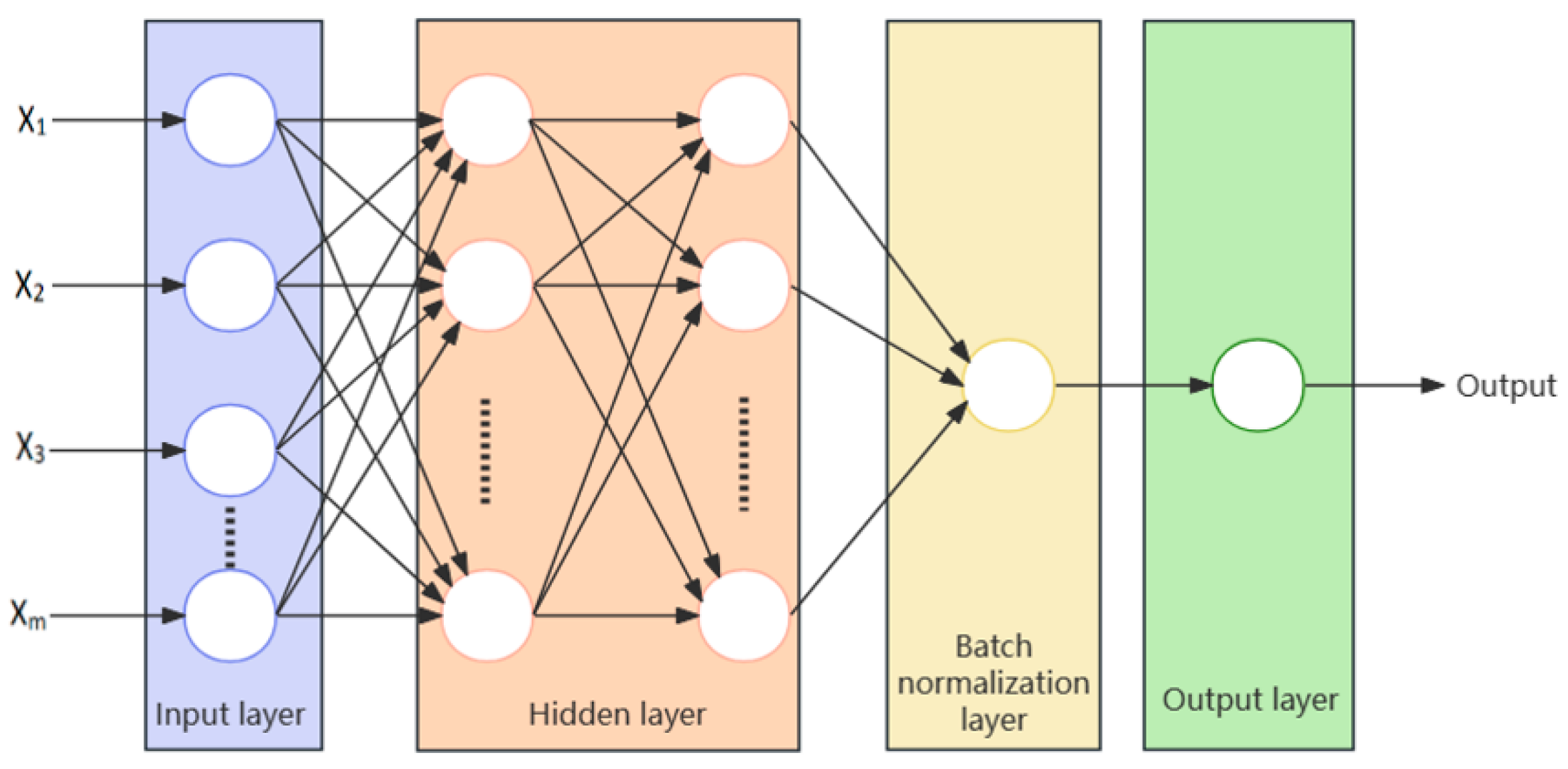
The training procedure of DNN is the same as BPNN, but the former has the following advantages: (1) it can learn complex nonlinear relationships; (2) features can be extracted automatically to train datasets of massive input parameters; (3) the expressive power of the model can be improved by increasing the number of hidden layers and neurons. The DNN model used in this research has five layers: one input layer, two hidden layers, one batch normalization layer, and one output layer. Specifically, the first, second, and third fully connected layers contain 19, 18, and 1 neuron, respectively. For model training, the number of epochs is set to 100, and the learning rate is configured as 0.001, as shown in Table 2. The structure diagram of the DNN model is shown in Figure 3. The DNN model is implemented with the framework of Deep Learning Toolbox in MATLAB R2024a.

4. Results

4.1. Correlation Analysis and Selection of Model Parameters

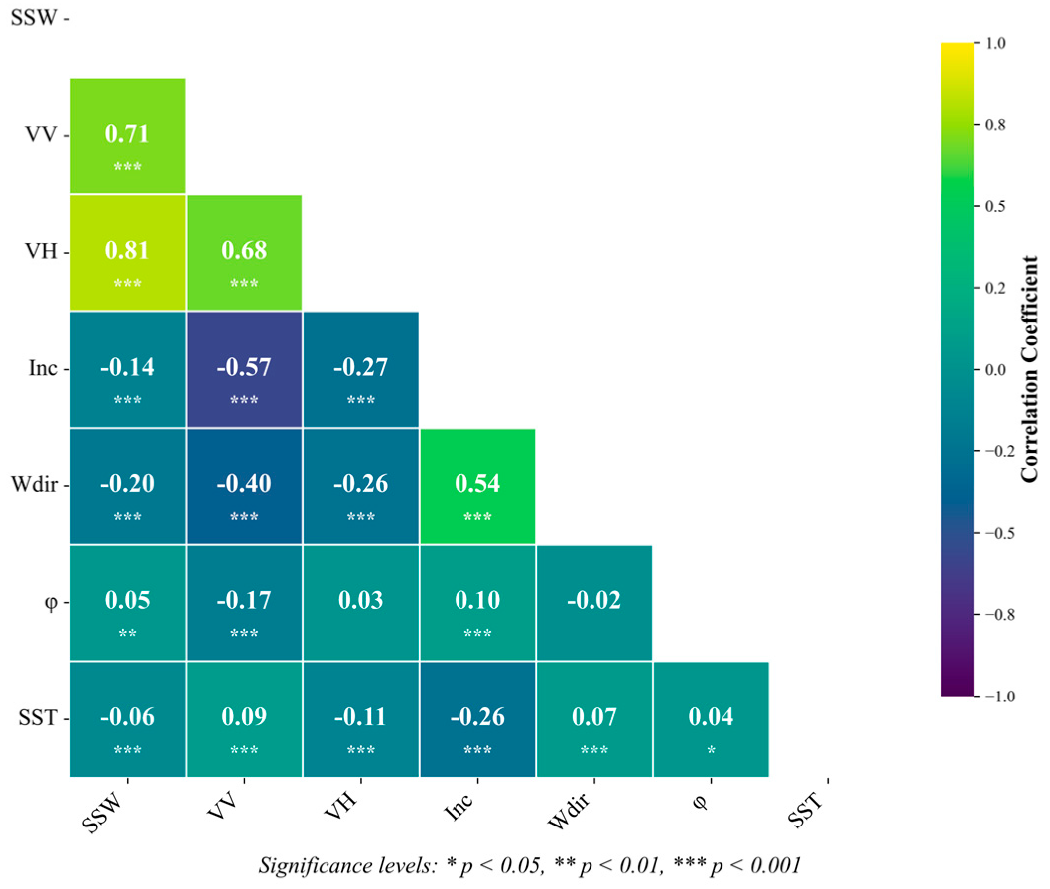
The selection of input parameters of models is very important in the process of establishing SSW retrieval models. This study uses the method of Pearson correlation analysis to analyze the correlation between SSW and different input parameters and further selects the RF model to test the influence of two input parameter combinations on the inversion results because of its advantages in solving classification problems and reducing overfitting. Both σ^VV and σ^VH show strong correlations with SSW, as shown in the correlation heatmap in Figure 4, with correlation coefficients larger than 0.7. Other parameters including SST also have correlations with SSW, although this is not so strong compared with dual-polarized SAR data.

The basic optional input parameters of the inversion model are σ^VV, σ^VH, Inc, Wdir, and φ. We build two combinations of model parameters for these five parameters, where the input parameters of RF-1 are σ^VV, σ^VH, and Wdir. RF-2 replaces Wdir by the relative angle φ between RLA and Wdir based on RF-1, which refers to the construction method of co-polarized CMOD models. The inversion results of the RF model with five basic input parameters are shown in

Table 3. The RF model results using different input parameters.

	Training Set				Validation Set				Test Set
	RMSE (m/s)	MAPE	CORR	Bias (m/s)	RMSE (m/s)	MAPE	CORR	Bias (m/s)	RMSE (m/s)	MAPE	CORR	Bias (m/s)
RF-1 (σVV, σVH, Inc, and Wdir)	1.40	3.79	0.98	0	1.00	3.36	0.99	0.02	3.40	10.63	0.94	−0.53
RF-2 (σVV, σVH, Inc, and φ)	1.25	3.30	0.99	0	0.78	2.76	0.99	−0.02	3.25	10.54	0.95	−0.26
RF-3 (σVV, σVH, Inc, φ, and SST)	0.93	2.07	0.99	0	0.50	1.81	0.99	−0.01	2.41	8.60	0.95	−0.39

, where the model evaluation indexes include RMSE, Mean Absolute Percentage error (MAPE), correlation coefficient (CORR), and bias index (Bias).

As can be seen from Table 3, when the input parameter of Wdir in RF-1 is replaced by φ in RF-2, the RMSE, MAPE, CORR, and Bias are almost all better than the RF-1 model on the training, validation, and test sets. The RMSE (3.25 m/s), MAPE (10.54%), CORR (0.95), and Bias (−0.26 m/s) are improved by 0.15 m/s, 0.09%, 0.01, and 0.27 m/s, respectively, showing better performance on the test set. The results show that orientation information in the form of the relative angle φ through inclusion of the RLA parameter, which are more closely related to SSW inversion, can improve the reliability of the model. Therefore, the basic parameter combinations of σ^VV, σ^VH, Inc, and φ, which are used in the RF-2 model, are used as the input parameters for the machine learning models in subsequent studies.

4.2. Inversion Results Based on Dual-Polarized SAR Data and Conventional Model Parameters

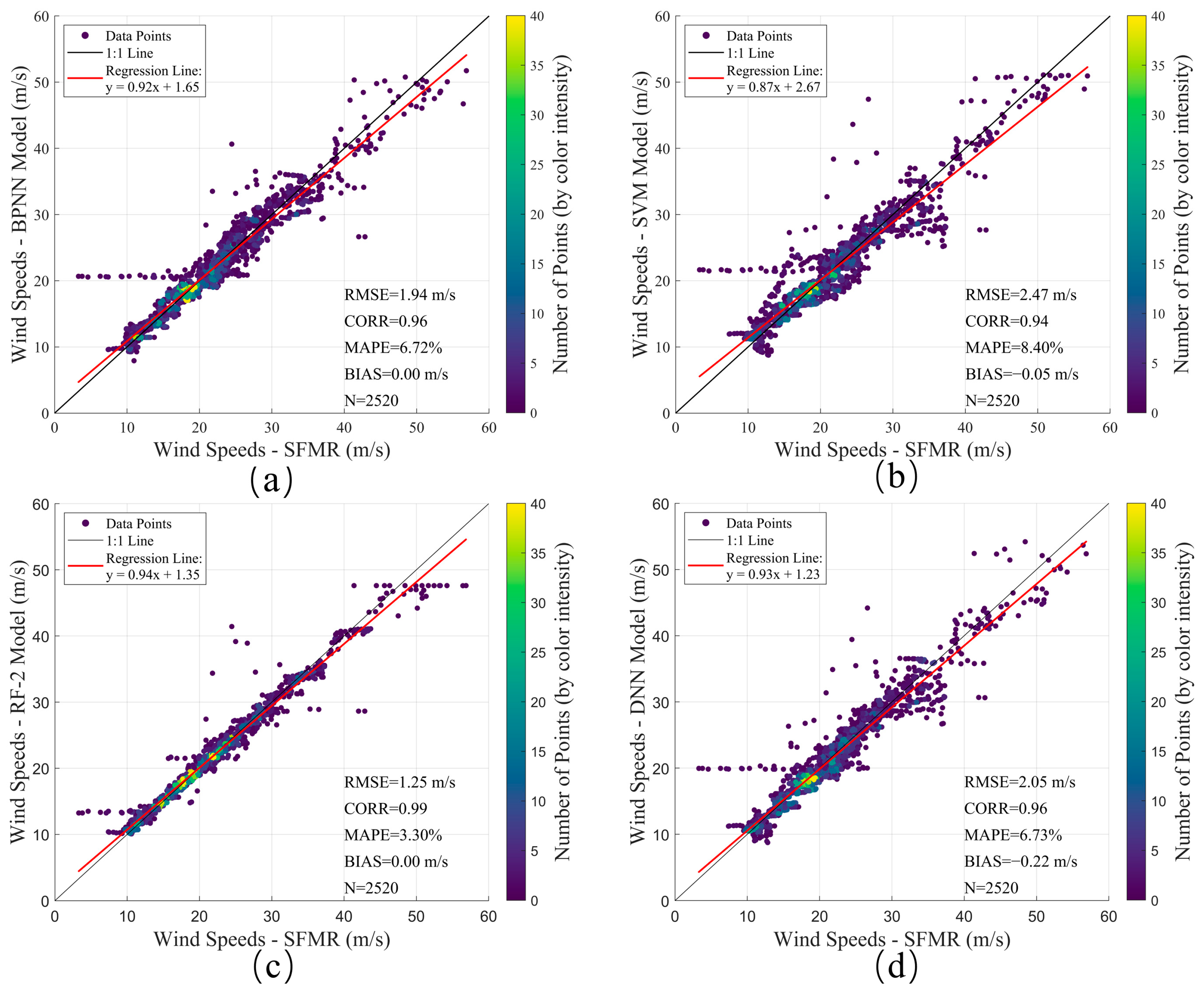
Using the feature combination of σ^VV, σ^VH, Inc, and φ, four SSW inversion models (BPNN, SVM, RF-2, and DNN) are finally obtained. Inversion results of these models on the training set are shown in Figure 5. The RF-2 model obtained the best statistical parameters of errors among four machine learning models, with a RMSE, MAPE, and CORR of 1.25 m/s, 3.30%, and 0.99, respectively. Exceptionally, similarly to the RF-2 model, the BPNN, trained with a bias <−0.01 m/s, also performed better than the DNN and SVM models. The DNN model achieved the largest absolute Bias (−0.22 m/s), whereas the SVM model achieved relatively worse results in terms of RMSE (2.47 m/s), MAPE (8.40%), and CORR (0.94).

Figure 6 shows the inversion results of the four machine learning models as well as the CMOD5.N model and S1IW.NR model on the validation set (N = 281). The RMSEs obtained by these four machine learning models are all less than 2.3 m/s. All these proposed models perform slightly better on the validation set than on the training set, probably because the validation set contains simpler and less ambiguous cases. Interestingly, the performance of these four machine learning models all outperform the traditional GMFs of CMOD5.N (5.16 m/s) and S1IW.NR (5.89 m/s). The RF-2 model obtains the lowest RMSE (0.78 m/s), outperforming the BPNN (1.50 m/s), SVM (2.23 m/s), and DNN (1.74 m/s) models. In addition, the RF-2 model obtains the lowest MAPE (2.76%), the highest CORR (0.99), and the smallest Bias (−0.02 m/s). The BPNN model again obtains better results than the DNN and SVM models, similar to the results on the training set. The DNN model has the worst bias of −0.34 m/s, while the SVM model achieves worse results for the RMSE, MAPE, and CORR. In contrast, the CMOD5.N model, with a bias of −3.01 m/s, greatly underestimates the SSW. The S1IW.NR model has a bias of 0.09 m/s, but it achieves the largest MAPE of 35.54%, which is 32.78% higher than the RF-2 model’s. The CMOD5.N model has the lowest CORR (0.71), which is 0.28 lower than the RF-2 model’s. We conclude that RF consistently shows the best performance among all models.

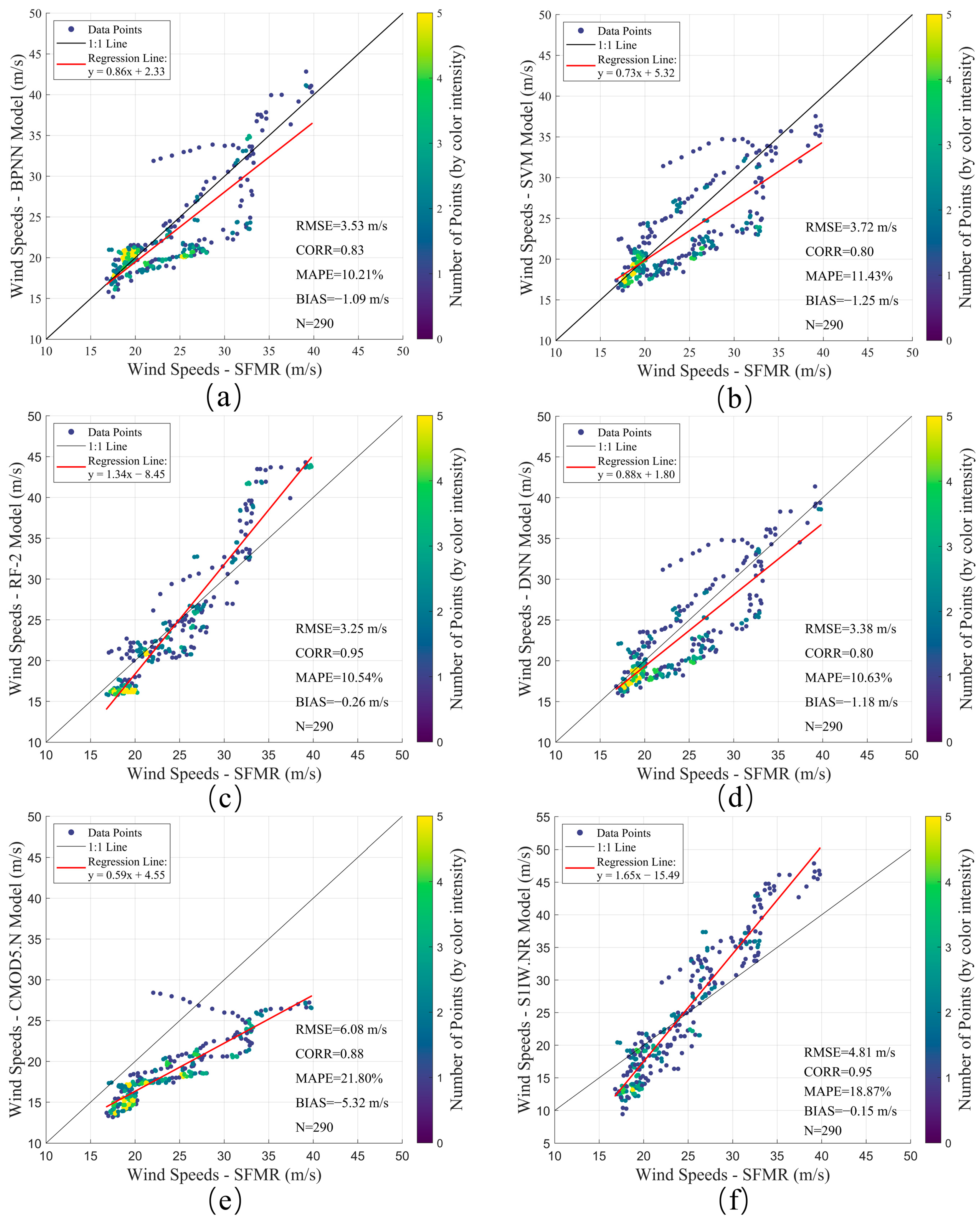
The S-1 SAR images of TC Dorian, acquired on 3 September 2019, and TC Micheal, acquired on 8 October 2018, are used as the test set to assess the generalization ability of the proposed machine learning models. The test data set consists of a total of 290 data points, which are independent of the training and validation sets. Figure 7 shows the retrieved SSWs by the four machine learning models (BPNN, SVM, RF, and DNN) and two traditional GMFs (CMOD5.N and S1IW.NR) on the test set compared with the SFMR wind data.

Among these four machine learning models, the RF-2 model exhibits the best generalization performance on the test set, obtaining the best results for RMSE (3.25 m/s), Bias (−0.26 m/s), and CORR (0.95), respectively. The DNN performs slightly worse than the RF-2 model with an RMSE of 3.38 m/s. The SVM model achieves the largest RMSE (3.72 m/s) and MAPE (11.43%), which are 0.47 m/s and 0.89% higher than the RF-2 model’s. Figure 7e,f show the inversion results for the CMOD5.N and S1IW.NR models. The CMOD5.N model obviously underestimates the SSW and obtains a very large error. The S1IW.NR model performs better than the CMOD5.N model and can achieve a smaller Bias, but it overestimates statistical parameters of RMSE and MAPE more than other machine learning methods. Overall, the RF-2 model using traditional model inputs can obtain the best results compared with other five different kinds of models.

4.3. Verification and Analysis of TCs Cases Based on RF Models

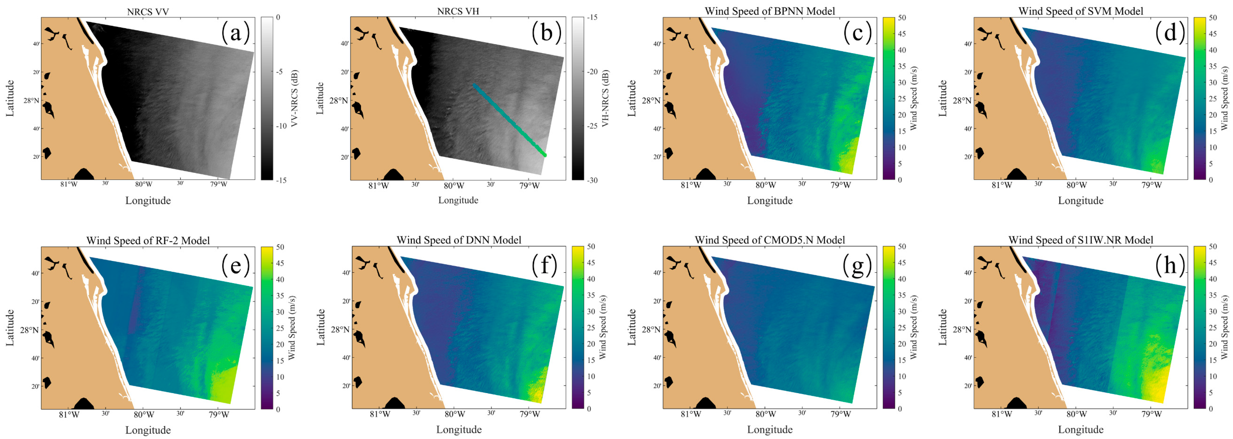
To compare the RF model with traditional GMFs using conventional model parameters, the wind field map from S-1 data of TC Dorian, which is independent from the training and validation data sets, is taken as an example. Figure 8a,b present the IW swath SAR images of TC Dorian from S-1 on 3 September 2019 in VV and VH polarizations by gray values (in dB), together with retrieved SSW maps by machine learning models (BPNN, SVM, RF, and DNN) and traditional GMFs (CMOD5.N and S1IW.NR), as shown in Figure 8c–h. These results are further compared along a cross section obtained from SFMR measurements, as shown in Figure 8b. Retrieved SSW values of RF-2, CMOD5.N, and S1IW.NR models along the same cross section are presented in Figure 9. The horizontal axis represents the distance between the sample point and the hurricane center, and the vertical axis represents the SSW value. Figure 9 shows that the CMOD5.N model always underestimates the SSW value and obtains the most significant error compared to other five models, whereas the S1IW.NR model overestimates the SSWs from the ~130 km mark to the typhoon center. Among machine learning models, the BPNN, SVM, and DNN models underestimate SSW results within a distance of ~80 to 150 km from the TC center. Overall, the RF-2 model shows better performance, with little difference in retrieved SSW values.

4.4. Performance of Different Models on High SSWs

Previous studies have shown that the input parameter of Wdir [31] or relative angle φ [26] can be used in dual-polarized models to obtain accurate SSWs during TCs. As shown in Table 3, RF-2, which incorporates the angle between Wdir and RLA, outperforms RF-1, which relies solely on Wdir. This study also demonstrates that machine learning models can substantially enhance the accuracy of high SSW inversion by using dual-polarized SAR data. The inversion results for 274 sample points with SSWs above 30 m/s are further calculated on the training set, as shown in

Table 4. Inversion results for samples with SSW values exceeding 30 m/s.

	RMSE (m/s)	MAPE (%)	CORR	Bias (m/s)
BPNN	6.21	14.00	0.33	2.34
SVM	5.50	13.65	0.76	4.03
RF-2	2.28	3.52	0.93	−0.93
RF-3	1.74	2.26	0.96	−0.58
DNN	5.11	12.59	0.72	3.25

. The RF-2 model achieves better overall statistics than the other models, whereas the DNN model outperforms BPNN and SVM in RMSE and MAPE. These results indicate that the DNN method may not be adapted for a relatively small data set with several thousand SSW sample points compared to RF. The BPNN model shows large fluctuations when the SSW is larger than 30 m/s, and has the worst performance in terms of RMSE, MAPE, and CORR. Except for the RF-2 model, the other three machine learning models may overfit in the process of adjusting the parameters at the beginning, leading to unstable inversion results after adjusting the parameters each time. Therefore, the complexity of these machine learning models should be reduced as much as possible to ensure inversion accuracy and stability. The inversion model based on RF performs better on the training set, which may be related to the fact that RF is composed of many decision trees, and different decision trees are not related to each other, which can effectively avoid the problem of overfitting, making the inversion results better than those of the other inversion models.

5. Discussion

5.1. Effect of SST on the Retrieved Model

The SSW manifesting in SAR images can also be affected by SST except for conventional input parameters in the inversion model [47]. Therefore, we propose the RF-3 model by including the SST parameter in the RF-2 model to explore the optimal parameter combination for SSW inversion models. The results show that the RF-3 model performs better than other machine learning models across all training, validation, and test sets, as shown in Table 4. The experiment results on the test set can also be seen in Figure 10. It can be observed that the inversion results of the RF-3 model obtain a notable improvement, with RMSE and MAPE decreasing by 0.84 m/s and 1.94%.

The performance of RF-3 is further examined along the same cross section, as shown in Figure 8b and Figure 9. The along-track SST data from SFMR measurements range from 28.6 °C to 29.7 °C, as presented in Figure 11, with higher temperatures observed at locations farther from the typhoon center. The SSW results calculated by the RF-3 model can be found in Figure 9, which includes the input feature of SST on the basis of RF-2. The RF-3 model further improves upon the performance of the RF-2 model, especially on the nearest sample points to the hurricane center. Overall, by introducing SST into the RF-3 model, it can better fit the SFMR SSWs compared to other models.

Under low SSW conditions, it was observed by Xu et al. [48] that a change of 1 °C in SST may lead to an error of 1–2 dB in the observed NRCS. This research indicates that SST can also impact wind retrievals under high SSW conditions above 30 m/s. RF-3, by introducing SST, can obtain better results than the RF-2 model for all four of these statistical parameters. It also presents the best generalization performance among all models according to the results on the test set. This result is consistent with previous research by analytic model simulations, in which wind retrieval errors due to SST could reach up to more than 0.4 m/s at 20 m/s [47]. Therefore, investigating SST effects on wind retrieval should be noted for related research in development of SSW inversion models using SAR data.

5.2. Effect of Rainfall Rate on Retrieved Model

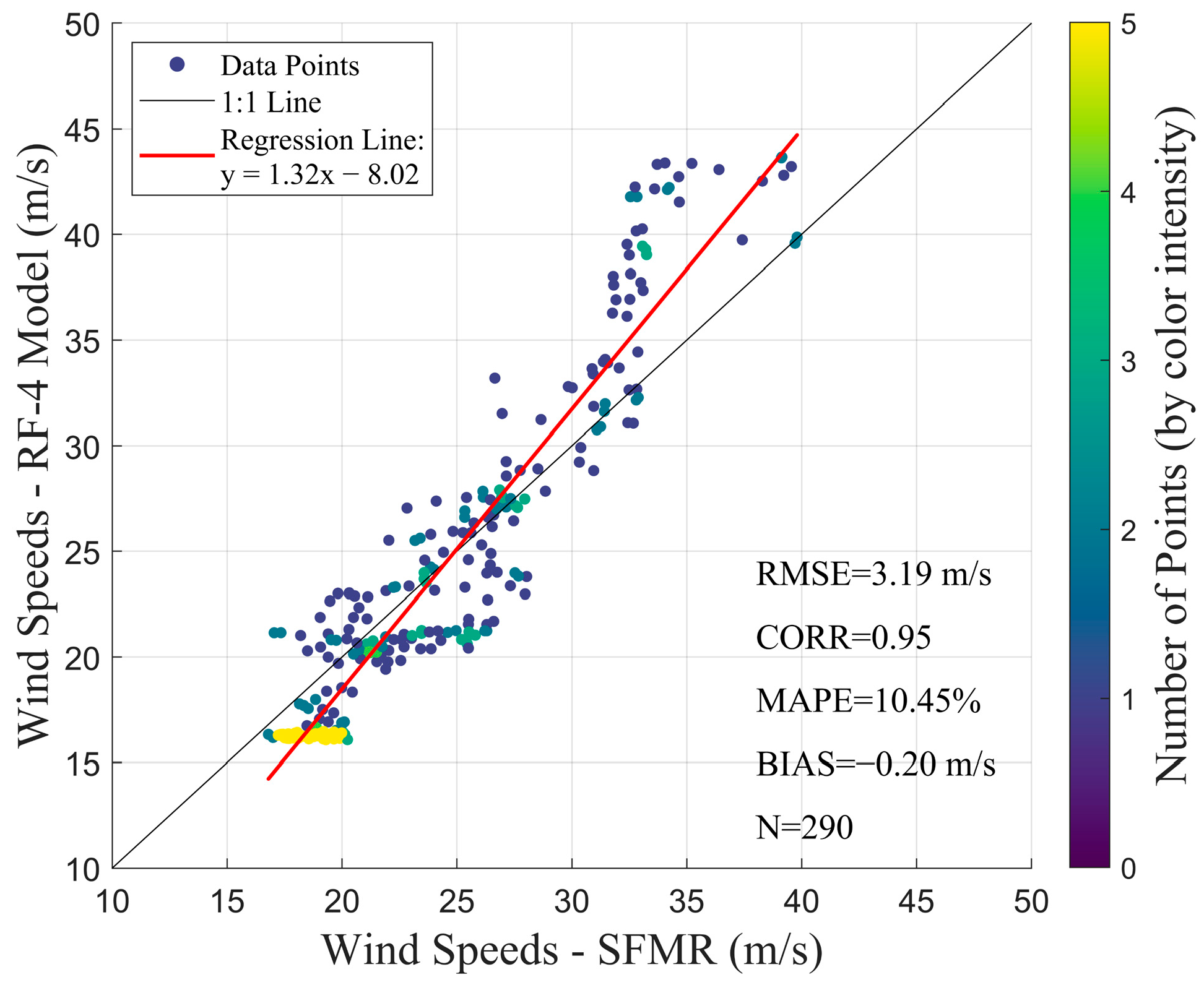
Previous studies have reported that rain over the ocean can impact features visible on SAR images [49,50]. The rain rate (ranging from 0 to 15 mm/h) along the cross section in Figure 8b can be seen in Figure 12. Moreover, it was found that the anomalous points with predicted SSWs around 20 m/s in Figure 5 are related to the rain rate. Therefore, this study further proposes the RF-4 model by including the rainfall parameter based on the RF-2 model to test the effect of rainfall on wind retrieval by machine learning models. The input parameters of RF-4 include σ^VV, σ^VH, Inc, φ, and rain rate. The inversion results of RF-4 on the test set are shown in Figure 13. It can perform slightly better than the RF-2 model (as shown in Figure 7c), with RMSE, MAPE, and CORR decreasing by 0.06 m/s, 0.09%, and 0.06 m/s. The results further demonstrate that the introduction of rain rate can improve the SSW retrieval model, which is consistent with previous studies, e.g., in [31,51].

6. Conclusions

This study develops several models based on machine learning and deep learning methods to retrieve TC SSW from collocated dual-polarized S-1 SAR images and SFMR measurements. The correlations between different model parameters and SSWs were explored through statistical analysis, and the RF algorithm, with its strong resistance to overfitting, was selected to establish four models with different input parameters. It was found that the RF-2 model with input parameters σ^VV, σ^VH, Inc, and φ exhibited better model performance and generalization ability. The RMSE obtained on the training, validation, and test sets were 1.25 m/s, 0.78 m/s, and 3.25 m/s, respectively. This result further determined the optimal combination of basic parameters. Then, the optimal parameter combination was used as input parameters for four machine learning models, BPNN, SVM, RF, and DNN, to train on a data set under TC conditions. The RF-2 model obtained the best SSW inversion results among different machine learning and traditional models on the test set. The impacts of SST on the inversion results were examined by introducing it in the RF-3 model. And it showed that the RF-3 model considering SST further optimized the inversion results on the test set. Finally, we validated and analyzed the wind field inversion of TC Dorian using different machine learning and traditional methods. The results proved that the RF-2 model using dual-polarized SAR data as its input more accurately restored true SSWs than other models. Using SFMR data as a reference, it was found that dual-polarized data and SST contribute to improving the inversions of SSWs by RF-3 in comparison with other models on the TC cross section. The results for RF-4 further demonstrated that the introduction of rain rate can improve SSW retrieval models.

Overall, the machine learning models based on the dual-polarized SAR data presented here are promising for obtaining SSWs. These methods may be applied to small SAR satellites and next-generation scatterometers in the inversion of TC wind speeds. The physical significance of the introduction of SST can be included in the future. Considering that velocity bunching can smear the SAR image [52], it is worth reducing its impact during the image processing procedure. The azimuthal cutoff wavelength induced by velocity bunching, which linearly correlates with SSW [53], could also be incorporated into the retrieval approach. In addition, we will collect more data under extreme wind conditions and improve the proposed machine learning models to explore their generalization ability to different conditions.

References

1. Yu, P.; Johannessen, J.A.; Yan, X.-H.; Geng, X.; Zhong, X.; Zhu, L. A Study of the Intensity of Tropical Cyclone Idai Using Dual-Polarization Sentinel-1 Data. Remote Sens. 2019, 11, 2837. [Google Scholar] [CrossRef]
2. Jing, R.; Heft-Neal, S.; Chavas, D.R.; Griswold, M.; Wang, Z.; Clark-Ginsberg, A.; Guha-Sapir, D.; Bendavid, E.; Wagner, Z. Global Population Profile of Tropical Cyclone Exposure from 2002 to 2019. Nature 2023, 626, 549–554. [Google Scholar] [CrossRef]
3. Gerling, T.W. Structure of the Surface Wind Field from the Seasat SAR. J. Geophys. Res. 1986, 91, 2308–2320. [Google Scholar] [CrossRef]
4. Sempreviva, A.M.; Barthelmie, R.J.; Pryor, S.C. Review of Methodologies for Offshore Wind Resource Assessment in European Seas. Surv. Geophys. 2008, 29, 471–497. [Google Scholar] [CrossRef]
5. Doubrawa, P.; Barthelmie, R.J.; Pryor, S.C.; Hasager, C.B.; Badger, M.; Karagali, I. Satellite Winds as a Tool for Offshore Wind Resource Assessment: The Great Lakes Wind Atlas. Remote Sens. Environ. 2015, 168, 349–359. [Google Scholar] [CrossRef]
6. Wan, Y.; Guo, S.; Li, L.; Qu, X.; Dai, Y. Data Quality Evaluation of Sentinel-1 and GF-3 SAR for Wind Field Inversion. Remote Sens. 2021, 13, 3723. [Google Scholar] [CrossRef]
7. Stoffelen, A.; Anderson, D. Scatterometer Data Interpretation: Estimation and Validation of the Transfer Function CMOD4. J. Geophys. Res. 1997, 102, 5767–5780. [Google Scholar] [CrossRef]
8. Hersbach, H.; Stoffelen, A.; De Haan, S. An Improved C-Band Scatterometer Ocean Geophysical Model Function: CMOD5. J. Geophys. Res. 2007, 112, C03006. [Google Scholar] [CrossRef]
9. Hersbach, H. Comparison of C-Band Scatterometer CMOD5.N Equivalent Neutral Winds with ECMWF. J. Atmos. Ocean. Technol. 2010, 27, 721–736. [Google Scholar] [CrossRef]
10. Stoffelen, A.; Verspeek, J.A.; Vogelzang, J.; Verhoef, A. The CMOD7 Geophysical Model Function for ASCAT and ERS Wind Retrievals. IEEE J. Sel. Top. Appl. Earth Obs. Remote Sens. 2017, 10, 2123–2134. [Google Scholar] [CrossRef]
11. Thompson, D.; Elfouhaily, T.; Chapron, B. Polarization Ratio for Microwave Backscattering from the Ocean Surface at Low to Moderate Incidence Angles. In Proceedings of the IEEE International Geoscience and Remote Sensing Symposium (IGARSS), Seattle, WA, USA, 6–10 July 1998; pp. 1671–1673. [Google Scholar]
12. Mouche, A.A.; Hauser, D.; Daloze, J.F.; Guerin, C. Dual-Polarization Measurements at C-Band over the Ocean: Results from Airborne Radar Observations and Comparison with ENVISAT ASAR Data. IEEE Trans. Geosci. Remote Sens. 2005, 43, 753–769. [Google Scholar] [CrossRef]
13. Donelan, M.A.; Haus, B.K.; Reul, N.; Plant, W.J.; Stiassnie, M.; Graber, H.C.; Brown, O.B.; Saltzman, E.S. On the Limiting Aerodynamic Roughness of the Ocean in Very Strong Winds. Geophys. Res. Lett. 2004, 31, L18306. [Google Scholar] [CrossRef]
14. Zhang, B.; Perrie, W. Cross-Polarized Synthetic Aperture Radar: A New Potential Measurement Technique for Hurricanes. Bull. Am. Meteorol. Soc. 2012, 93, 531–541. [Google Scholar] [CrossRef]
15. Hwang, P.A.; Stoffelen, A.; van Zadelhoff, G.; Perrie, W.; Zhang, B.; Li, H.; Shen, H. Cross-Polarization Geophysical Model Function for C-Band Radar Backscattering from the Ocean Surface and Wind Speed Retrieval. J. Geophys. Res. Ocean. 2015, 120, 893–909. [Google Scholar] [CrossRef]
16. Zhang, G.; Li, X.; Perrie, W.; Hwang, P.A.; Zhang, B.; Yang, X. A Hurricane Wind Speed Retrieval Model for C-Band RADARSAT-2 Cross-Polarization ScanSAR Images. IEEE Trans. Geosci. Remote Sens. 2017, 55, 4766–4774. [Google Scholar] [CrossRef]
17. Zhang, T.; Li, X.M.; Feng, Q.; Ren, Y.; Shi, Y. Retrieval of Sea Surface Wind Speeds from Gaofen-3 Full Polarimetric Data. Remote Sens. 2019, 11, 813. [Google Scholar] [CrossRef]
18. Gao, Y.; Sun, J.; Zhang, J.; Guan, C. Extreme Wind Speeds Retrieval Using Sentinel-1 IW Mode SAR Data. Remote Sens. 2021, 13, 1867. [Google Scholar] [CrossRef]
19. Horstmann, J.; Falchetti, S.; Wackerman, C.; Maresca, S.; Caruso, M.J.; Graber, H.C. Tropical Cyclone Winds Retrieved from C-Band Cross-Polarized Synthetic Aperture Radar. IEEE Trans. Geosci. Remote Sens. 2015, 53, 2887–2898. [Google Scholar] [CrossRef]
20. Sun, Y.; Li, X.M. Denoising Sentinel-1 Extra-Wide Mode Cross-Polarization Images Over Sea Ice. IEEE Trans. Geosci. Remote Sens. 2021, 59, 2116–2131. [Google Scholar] [CrossRef]
21. Park, J.W.; Won, J.S.; Korosov, A.A.; Babiker, M.; Miranda, N. Textural Noise Correction for Sentinel-1 TOPSAR Cross-Polarization Channel Images. IEEE Trans. Geosci. Remote Sens. 2019, 57, 4040–4049. [Google Scholar] [CrossRef]
22. Ye, X.; Lin, M.; Zheng, Q.; Yuan, X.; Liang, C.; Zhang, B.; Zhang, J. A Typhoon Wind-Field Retrieval Method for the Dual-Polarization SAR Imagery. IEEE Geosci. Remote Sens. Lett. 2019, 16, 1511–1515. [Google Scholar] [CrossRef]
23. Portabella, M.; Stoffelen, A.; Johannessen, J.A. Toward an Optimal Inversion Method for Synthetic Aperture Radar Wind Retrieval. J. Geophys. Res. 2002, 107, C08011. [Google Scholar] [CrossRef]
24. Jiang, Z.; Li, Y.; Yu, F.; Chen, G.; Yu, W. A Damped Newton Variational Inversion Method for SAR Wind Retrieval. J. Geophys. Res. Atmos. 2017, 122, 823–845. [Google Scholar] [CrossRef]
25. Mouche, A.A.; Chapron, B.; Zhang, B.; Husson, R. Combined Co- and Cross-Polarized SAR Measurements Under Extreme Wind Conditions. IEEE Trans. Geosci. Remote Sens. 2017, 55, 6746–6755. [Google Scholar] [CrossRef]
26. Mouche, A.; Chapron, B.; Knaff, J.; Zhao, Y.; Zhang, B.; Combot, C. Copolarized and Cross-Polarized SAR Measurements for High-Resolution Description of Major Hurricane Wind Structures: Application to Irma Category 5 Hurricane. J. Geophys. Res. Ocean. 2019, 124, 3905–3922. [Google Scholar] [CrossRef]
27. Gao, Y.; Wang, Y.; Wang, W. A New Approach for Ocean Surface Wind Speed Retrieval Using Sentinel-1 Dual-Polarized Imagery. Remote Sens. 2023, 15, 4267. [Google Scholar] [CrossRef]
28. Zhao, T.; Wang, S.; Ouyang, C.; Chen, M.; Liu, C.; Zhang, J.; Yu, L.; Wang, F.; Xie, Y.; Li, J.; et al. Artificial Intelligence for Geoscience: Progress, Challenges, and Perspectives. Innovation 2024, 5, 100691. [Google Scholar] [CrossRef]
29. Horstmann, J.; Schiller, H.; Schulz-Stellenfleth, J.; Lehner, S. Global Wind Speed Retrieval from SAR. IEEE Trans. Geosci. Remote Sens. 2003, 41, 2277–2286. [Google Scholar] [CrossRef]
30. Qin, T.; Jia, T.; Feng, Q.; Li, X. Sea Surface Wind Speed Retrieval from Sentinel-1 HH Polarization Data Using Conventional and Neural Network Methods. Acta Oceanol. Sin. 2021, 40, 13–21. [Google Scholar] [CrossRef]
31. Mu, S.; Li, X.; Wang, H. The Fusion of Physical, Textural, and Morphological Information in SAR Imagery for Hurricane Wind Speed Retrieval Based on Deep Learning. IEEE Trans. Geosci. Remote Sens. 2022, 60, 4207513. [Google Scholar] [CrossRef]
32. Yu, P.; Xu, W.; Zhong, X.; Johannessen, J.A.; Yan, X.-H.; Geng, X.; He, Y.; Lu, W. A Neural Network Method for Retrieving Sea Surface Wind Speed for C-Band SAR. Remote Sens. 2022, 14, 2269. [Google Scholar] [CrossRef]
33. Hu, Y.; Shao, W.; Shen, W.; Zhou, Y.; Jiang, X. Machine Learning Applied to a Dual-Polarized Sentinel-1 Image for Wind Retrieval of Tropical Cyclones. Remote Sens. 2023, 15, 3948. [Google Scholar] [CrossRef]
34. Sato, N.; Shirooka, R.; Yoshizaki, M.; Takayabu, Y.N. Meridional SST Gradient in The Western North Pacific Warm Pool Associated with Typhoon Generation. Geophys. Res. Lett. 2008, 35, L12803. [Google Scholar] [CrossRef]
35. Clemente-Colon, P.; Yan, X.-H. Observations of East Coast Upwelling Conditions in Synthetic Aperture Radar Imagery. IEEE Trans. Geosci. Remote Sens. 1999, 37, 2239–2248. [Google Scholar] [CrossRef]
36. Kim, T.-S.; Park, K.-A.; Li, X.; Mouche, A.A.; Chapron, B.; Lee, M. Observation of Wind Direction Change on the Sea Surface Temperature Front Using High-Resolution Full Polarimetric SAR Data. IEEE J. Sel. Top. Appl. Earth Obs. Remote Sens. 2017, 10, 2599–2607. [Google Scholar] [CrossRef]
37. Liu, G.Q.; Perrie, W.; Kudryavtsev, V.; He, Y.; Shen, H.; Zhang, B.; Hu, H. Radar Imaging of Intense Nonlinear Ekman Divergence. Geophys. Res. Lett. 2016, 43, 9810–9818. [Google Scholar] [CrossRef]
38. Bentamy, A.; Grodsky, S.A.; Carton, J.A.; Croize-Fillon, D.; Chapron, B. Matching ASCAT and QuikSCAT Winds. J. Geophys. Res. Ocean. 2012, 117, C02011. [Google Scholar] [CrossRef]
39. Grodsky, S.A.; Kudryavtsev, V.N.; Bentamy, A.; Carton, J.A.; Chapron, B. Does Direct Impact of SST on Short Wind Waves Matter for Scatterometry? Geophys. Res. Lett. 2012, 39, L12602. [Google Scholar] [CrossRef]
40. Wang, Z.; Stoffelen, A.; Zhao, C.; Vogelzang, J.; Verhoef, A.; Verspeek, J. An SST-Dependent Ku-Band Geophysical Model Function for RapidScat. J. Geophys. Res. Ocean. 2017, 122, 3461–3480. [Google Scholar] [CrossRef]
41. Uhlhorn, E.W.; Black, P.G.; Franklin, J.L.; Goodberlet, M.; Carswell, J.; Goldstein, A.S. Hurricane Surface Wind Measurements. from an Operational Stepped Frequency Microwave Radiometer. Mon. Weather Rev. 2007, 135, 3070–3085. [Google Scholar] [CrossRef]
42. Klotz, B.W.; Uhlhorn, E.W. Improved Stepped Frequency Microwave Radiometer Tropical Cyclone Surface Winds in Heavy Precipitation. J. Atmos. Ocean. Technol. 2014, 31, 2392–2408. [Google Scholar] [CrossRef]
43. Zhang, K.; Huang, J.; Xu, X.; Guo, Q.; Chen, Y.; Mansaray, L.R.; Li, Z.; Wang, X. Spatial Scale Effect on Wind Speed Retrieval Accuracy Using Sentinel-1 Copolarization SAR. IEEE Geosci. Remote Sens. Lett. 2018, 15, 882–886. [Google Scholar] [CrossRef]
44. Wang, S.; Yuen, K.V.; Yang, X.F.; Zhang, B. A Nonparametric Tropical Cyclone Wind Speed Estimation Model Based on Dual-Polarization SAR Observations. IEEE Trans. Geosci. Remote Sens. 2022, 60, 4208213. [Google Scholar] [CrossRef]
45. Yang, G.G.; Wang, Q.; Feng, J.; He, L.; Li, R.; Lu, W.; Liao, E.; Lai, Z. Can Three-Dimensional Nitrate Structure Be Reconstructed from Surface Information with Artificial Intelligence?—A Proof-of-Concept Study. Sci. Total Environ. 2024, 924, 171365. [Google Scholar] [CrossRef]
46. Lu, W.; Su, H.; Yang, X.; Yan, X.-H. Subsurface Temperature Estimation from Remote Sensing Data Using a Clustering-Neural Network Method. Remote Sens. Environ. 2019, 229, 213–222. [Google Scholar] [CrossRef]
47. Du, Y.; Yang, X.; Yang, J.; Tan, S.; Ma, W.; Li, Z.; Li, X. Effects of Temperature on Sea Surface Radar Backscattering Under Neutral and Nonneutral Atmospheric Conditions for Wind Retrieval Applications: A Numerical Study. IEEE Trans. Geosci. Remote Sens. 2021, 59, 2727–2743. [Google Scholar] [CrossRef]
48. Xu, Q.; Li, Y.; Li, X.; Zhang, Z.; Cao, Y.; Cheng, Y. Impact of Ships and Ocean Fronts on Coastal Sea Surface Wind Measurements From the Advanced Scatterometer. IEEE J. Sel. Top. Appl. Earth Obs. Remote Sens. 2018, 11, 2162–2169. [Google Scholar] [CrossRef]
49. Alpers, W.; Zhang, B.; Mouche, A.A.; Zeng, K.; Chan, P.K. Rain Footprints on C-Band Synthetic Aperture Radar Images of the Ocean—Revisited. Remote Sens. Environ. 2016, 187, 169–185. [Google Scholar] [CrossRef]
50. Guo, C.; Ai, W.; Zhang, X.; Guan, Y.; Liu, Y.; Hu, S. Correction of Sea Surface Wind Speed Based on SAR Rainfall Grade Classification Using Convolutional Neural Network. IEEE J. Sel. Top. Appl. Earth Obs. Remote Sens. 2023, 16, 321–328. [Google Scholar] [CrossRef]
51. Zhang, B.; Mouche, A.A.; Perrie, W. First Quasi-Synchronous Hurricane Quad-Polarization Observations by C-Band Radar Constellation Mission and RADARSAT-2. IEEE Trans. Geosci. Remote Sens. 2022, 60, 4206510. [Google Scholar] [CrossRef]
52. Corcione, V.; Grieco, G.; Portabella, M.; Nunziata, F.; Migliaccio, M. A Novel Azimuth Cutoff Implementation to Retrieve Sea Surface Wind Speed From SAR Imagery. IEEE Trans. Geosci. Remote Sens. 2019, 57, 3331–3340. [Google Scholar] [CrossRef]
53. Grieco, G.; Lin, W.; Migliaccio, M.; Nirchio, F.; Portabella, M. Dependency of the Sentinel-1 azimuth wavelength cut-off on significant wave height and wind speed. Int. J. Remote Sens. 2016, 37, 5086–5104. [Google Scholar] [CrossRef]
Figure 1. The S-1 SAR image of TC Dorian, acquired on 27 August 2019, before (a) and after (b) denoising in the VH channel.
Remotesensing 17 03626 g001
Figure 2. (a) Histogram of SSWs and (b) radar incidence angles for the matching data set.
Remotesensing 17 03626 g002
Figure 3. Structure of the DNN model.
Remotesensing 17 03626 g003
Figure 4. The correlation heatmap between different input parameters and SSW.
Remotesensing 17 03626 g004
Figure 5. Model results from the training set by the (a) BPNN model, (b) SVM model, (c) RF-2 model, and (d) DNN model, where the horizontal coordinate is the SSW value provided by SFMR, the vertical coordinate is the retrieved SSW value, and the colormap represents the density of sample points.
Remotesensing 17 03626 g005
Figure 6. Model results from the validation set by (a) BPNN model, (b) SVM model, (c) RF-2 model, (d) DNN model, (e) COMD5.N model, and (f) S1IW.NR model.
Remotesensing 17 03626 g006
Figure 7. Model results from the independent test data set by (a) BPNN model, (b) SVM model, (c) RF-2 model, (d) DNN model, (e) COMD5.N model, and (f) S1IW.NR model.
Remotesensing 17 03626 g007
Figure 8. TC Dorian captured by independent S-1 dual-polarized SAR image at 11:17 UTC on 3 September 2019 showing (a) VV polarized SAR image, (b) VH polarized SAR image, and SSW retrievals from (c) BPNN, (d) SVM, (e) RF-2, (f) DNN, (g) CMOD5.N, and (h) S1IW.NR models.
Remotesensing 17 03626 g008
Figure 9. Comparisons of different SSW results retrieved by two traditional GMFs (CMOD5.N and S1IW.NR) and proposed four kinds of machine learning models along the cross section shown in Figure 8b.
Remotesensing 17 03626 g009
Figure 10. Model results considering SST from the independent validation data set by the RF-3 model.
Remotesensing 17 03626 g010
Figure 11. The variations in SST along the SFMR track (as seen in Figure 8b) collocated with S-1 SAR data of TC Dorian acquired on 3 September 2019.
Remotesensing 17 03626 g011
Figure 12. The variations in rain rate along the SFMR track (as seen in Figure 8b) collocated with S-1 SAR data of TC Dorian acquired on 3 September 2019.
Remotesensing 17 03626 g012
Figure 13. Model results considering rain rate from the independent validation data set by the RF-4 model.
Remotesensing 17 03626 g013