Highlights
What are the main findings?
- This study introduces a nonlinear spectral unmixing, which captures sub-pixel benthic habitat composition.
- Unmixing provides more ecologically realistic reef mapping than higher-accuracy ML models.
What are the implications of the main findings?
- This study enables scalable reef mapping using multispectral data without site-specific inputs.
- Sub-pixel outputs enhance reef monitoring by revealing fine-scale habitat composition.
Abstract
Accurate, scalable mapping of coral reef habitats is essential for monitoring ecosystem health and detecting change over time. In this study, we introduce a novel mathematically based nonlinear spectral unmixing method for benthic habitat classification, which provides sub-pixel estimates of benthic composition, capturing the mixed benthic composition within individual pixels. We compare its performance against two machine learning approaches: semi-supervised K-Means clustering and AdaBoost decision trees. All models were applied to high-resolution PlanetScope satellite imagery and ICESat-2-derived terrain metrics. Models were trained using a ground truth dataset constructed from benthic photoquadrats collected at Heron Reef, Australia, with additional input features including band ratios, standardized band differences, and derived ICESat-2 metrics such as rugosity and slope. While AdaBoost achieved the highest overall accuracy () and benefited most from ICESat-2 features, K-Means performed less well () and declined when these metrics were included. The spectral unmixing method uniquely captured sub-pixel habitat abundance, offering a more nuanced and ecologically realistic view of reef composition despite lower discrete classification accuracy (). These findings highlight nonlinear spectral unmixing as a promising approach for fine-scale, transferable coral reef habitat mapping, especially in complex or heterogeneous reef environments.
1. Introduction
Coral reefs are among the most biodiverse and ecologically important ecosystems in the world. The Great Barrier Reef, recognized as one of the Seven Natural Wonders of the World, supports an estimated 9000 marine species, contributing to one of the highest levels of biological variability found in marine environments [1]. Beyond their ecological value, coral reefs play a critical role in protecting coastlines by reducing wave energy from storms and sustaining local economies through fisheries and tourism. The Great Barrier Reef alone generates approximately A$6.4 billion annually for Australia’s economy and supports around 64,000 jobs [2]. However, coral reef ecosystems are under increasing threat from climate change and anthropogenic pressures, including rising sea surface temperatures, ocean acidification, pollution, and overfishing. From 1982–2012, the Great Barrier Reef lost nearly half of its coral cover [3], a decline that underscores the urgency of implementing large-scale mapping and monitoring strategies.
Remote sensing has emerged as an invaluable tool for coral reef mapping, offering a non-invasive, cost-effective, and efficient method of collecting data across large spatial extents. Among the various remote sensing platforms used for reef monitoring, satellite imagery is especially useful, enabling consistent and detailed assessments of reef health, biodiversity, and environmental change. Multispectral and hyperspectral imaging, in particular, captures information across a range of spectral wavelengths, allowing for the identification of geomorphic zones and, at appropriate spatial and spectral resolutions, biological cover types such as live coral, macroalgae, and sand [4]. Numerous studies have demonstrated the utility of satellite imagery in reef applications, including the use of Landsat for long-term monitoring of reef health and changes in coral cover [5,6], Sentinel-2 for moderate-resolution habitat mapping [7,8], and high-resolution platforms like PlanetScope satellites for fine-scale analysis of reef structure and composition [9,10].
To extract ecological insights from remote sensing data, researchers typically apply classification algorithms that translate spectral and environmental information into habitat maps. Machine learning (ML) has become the most prevalent approach for this task. Supervised ML methods such as maximum likelihood classification [11,12], support vector machines [13], and random forests [14] are among the most commonly used to classify benthic zones and biological cover. Species distribution models such as maximum entropy (MaxEnt) are also used to predict the spatial distribution of individual species [15]. These approaches rely on labeled training data to learn relationships between spectral and environmental features and the habitat classes of interest. Although satellite-based benthic habitat mapping has been practiced for decades, recent improvements in remote sensing technology and classification methods have substantially enhanced its effectiveness.
Another technique, spectral unmixing, addresses the inherent complexity of reef environments by estimating the fractional composition of multiple classes within a pixel. This approach, widely used in land cover mapping and mineral exploration, is especially valuable in mixed-pixel environments such as coral reefs, where fine-scale ecological variation is often indistinguishable by satellite imagery due to the spatial resolution. Unlike classification methods that assign a single label per pixel, linear spectral unmixing estimates the abundances of multiple known “endmembers” (or classes) within each pixel, producing fractional maps of benthic composition. Many existing spectral unmixing approaches for reef mapping rely on water column corrections to retrieve seafloor reflectance from satellite imagery [16,17]. Others use semi-analytical bio-optical models—most notably the model developed by Lee et al. [18,19]—to estimate water column properties such as depth, absorption, and backscatter, which can then be used to aid in unmixing [20,21]. However, both approaches require site-specific environmental parameters, which can limit model transferability and complicate large-scale applications across diverse reef systems. These methods typically rely on hyperspectral data to exploit narrow spectral bands that enable class separability. However, their dependence on site-specific environmental parameters and the limited availability of hyperspectral imagery at high spatial resolution present challenges for broad-scale reef mapping.
In contrast, few studies have explored spectral unmixing using multispectral data in reef settings without applying water column corrections [16,22]. This study contributes to this emerging area by developing and applying a novel nonlinear unmixing approach that operates directly on high-resolution multispectral imagery without explicit correction for water column effects. We further explore the benefits of incorporating complementary remote sensing data. Specifically, the Ice, Cloud, and land Elevation Satellite-2 (ICESat-2) provides photon-counting lidar data, which we use to derive terrain metrics such as slope, rugosity, and depth [23]. This topographic information may help to better distinguish benthic cover types. Furthermore, we evaluate the extent to which ICESat-2-derived metrics improve classification results. By avoiding the need for in situ water column measurements, this approach enhances model robustness and scalability for reef environments and decreases the cost of data acquisition.
This study evaluates and compares three approaches to coral reef habitat mapping using high-resolution satellite imagery and ICESat-2-derived topographic metrics: semi-supervised K-Means clustering, AdaBoost decision trees, and our novel nonlinear spectral unmixing model. We assess the performance of each method, both with and without ICESat-2 inputs, to determine how additional data influence classification outcomes. We also explore the trade-offs between discrete and fractional mapping approaches. Ultimately, this work informs future strategies for large-scale reef mapping and demonstrates how combining spectral and terrain-specific data can improve habitat classification in complex benthic environments.
2. Materials and Methods
2.1. Study Area
Our research focused on the coral cay of Heron Island, situated at the southern tip of Australia’s Great Barrier Reef (Figure 1). Heron Reef is geographically located at 23°27′S. Lat., 151°57′E. Lon. This atoll reef is recognized for its exceptional biodiversity, supporting 72% of all coral species found on the Great Barrier Reef. Its relatively shallow depth and consistently clear waters make it an ideal site for remote sensing applications, offering favorable conditions for testing methodologies in benthic composition mapping.
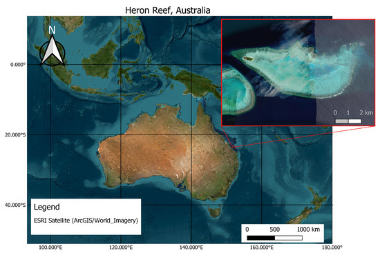
Figure 1.
Satellite image of Heron Island and the surrounding Heron Reef, Australia. Map lines delineate the study area and do not necessarily represent accepted national boundaries. Background imagery is derived from ESRI basemaps.
2.2. PlanetScope Satellite Imagery
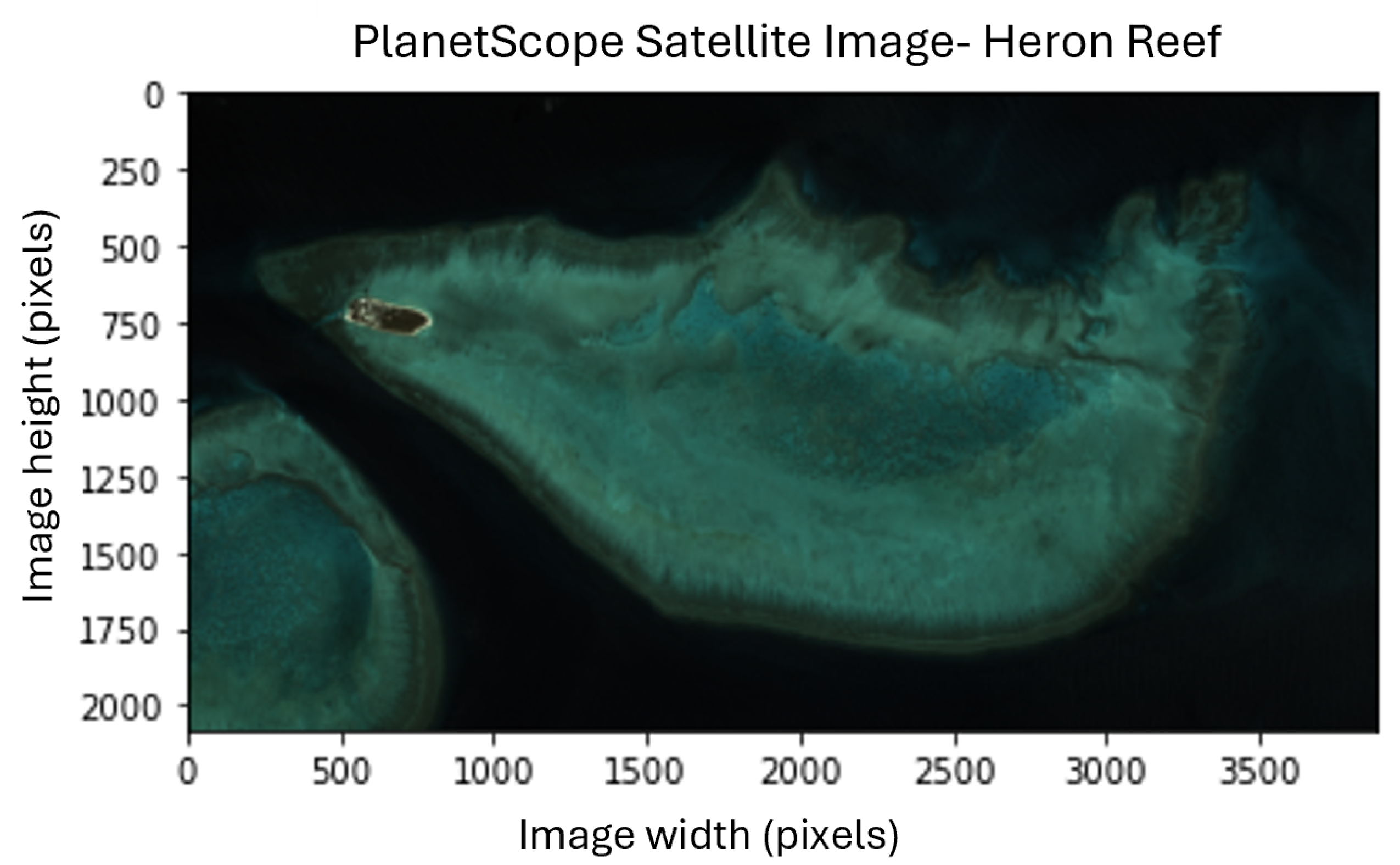
Planet, with its mission to “image the Earth every day,” collaborates with businesses, governments, and research institutions to harness satellite data for addressing global challenges. The company’s PlanetScope satellite constellation, consisting of approximately 120 satellites, captures multispectral images with a high spatial resolution of 3 m pixels. These images are captured as continuous strips of individual frames that are stitched together to form seamless scenes. With hundreds of satellites orbiting the planet approximately every 90 min, Planet provides near real-time global coverage. For this study, we utilized a PlanetScope Scene (PSScene) from October 2018 over Heron Reef (S. Lat., E. Lon.), located at the southern end of the Great Barrier Reef, Queensland, Australia (Figure 2) [24]. The scene contains four multispectral bands: blue, green, red, and near-infrared (NIR). This date was selected as it closely aligned with the ground truth data collection period. The delivered PSScene was provided as Analytic Surface Reflectance, which Planet orthorectified, calibrated, and atmospherically corrected. The reflectance values were scaled by a factor of 10,000, such that the raw data range from 0 to 10,000 corresponds to a physical surface reflectance of 0–1 [25]. Using the NIR band, the image was assessed for sunglint, but the correction was determined to have minimal effect; therefore, no further adjustments were applied.
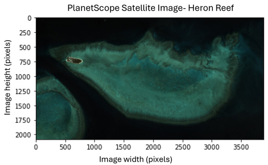
Figure 2.
PlanetScope satellite image of Heron Island acquired on 24 October 2018, displayed using the RGB bands in pixel coordinates (image width and height).
2.3. Roelfsema Photoquadrats
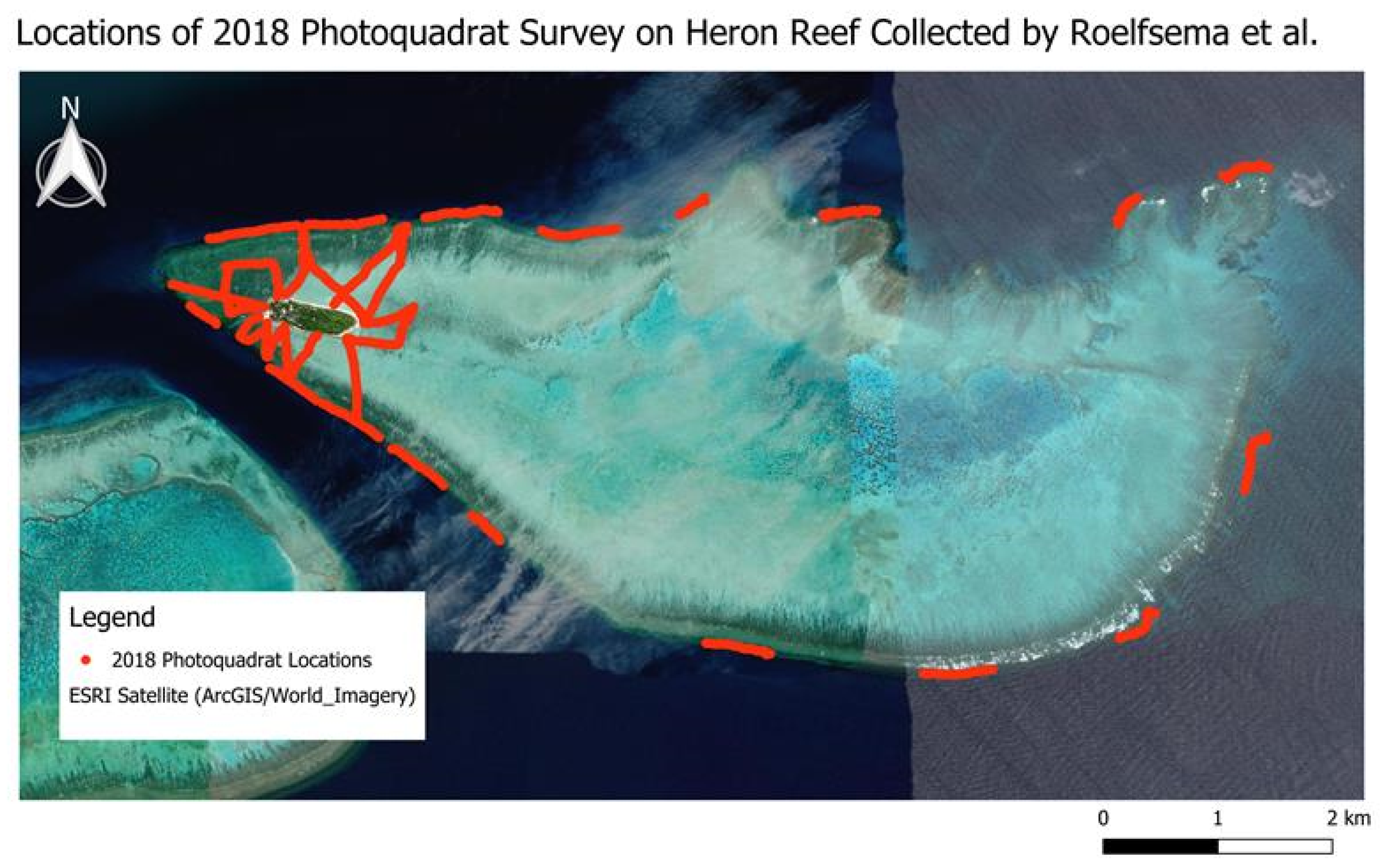
Roelfsema et al. [26] provide a dataset of underwater benthic photos collected during a photo-transect survey of the Great Barrier Reef, including Heron Reef, between 11 and 16 November 2018. The survey used a systematic layout of m photoquadrats spaced approximately 2–4 m apart. Each image was captured orthogonal to the seafloor from a height of m, with GPS coordinates marking the center of each quadrat [27]. The 2018 dataset includes 5544 georeferenced photoquadrats across the Heron Reef atoll, covering reef flat, crest, and slope habitats (Figure 3). Each photoquadrat was labeled with quantitative benthic and substrate cover data derived from field photo-transect surveys. The benthic labels in this dataset are detailed at the genus and species levels, and the associated percent cover values reflect the proportion of the quadrat occupied by each benthic type. Given that the satellite imagery was collected in October 2018, we assumed benthic community composition remained stable between October and November. This dataset played a critical role in developing a ground truth dataset used for testing and training ML models in this study.

Figure 3.
Spatial distribution of all 5544 photoquadrats collected over Heron Reef during the 2018 Roelfsema et al. photo-transect survey [26].
2.4. ICESat-2 Data
ICESat-2, containing the Advanced Topographic Laser Altimeter System (ALTAS) photon-counting instrument, utilizes a green laser (532 nm) to collect Earth elevation data. At each overpass, this laser surveys three pairs of beams spaced 3.3 km apart, where each pair contains a strong and a weak transmit energy beam spaced 90 m apart, resulting in six beams total. The strong and weak beams differ in transmit energies with an approximate ratio of 4:1. With a footprint width of approximately km across track, ICESat-2 releases 10,000 photon events (PEs) per second, ideally providing a ground-based measurement every 70 cm on the strong tracks and 280 cm on the weak tracks [28]. Twenty-three distinct ICESat-2 tracks from eight different dates (2019–2022) were used in the study.
This study incorporated algorithmically derived terrain-specific parameters extracted from ICESat-2 data (i.e., rugosity, slope, and depth), as explained in [23]. These variables were derived from ICESat-2’s data product ATL03, Global Geolocated Photons [29], and interpolated to generate a continuous surface covering the entire study area. Details on this method and the parameters extracted can be found in Section 2.7.2, and the resulting interpolated surfaces are provided in Appendix A for reference. The ICESat-2 data were incorporated into both the pure pixel library (used as ground truth) and the raster data from the satellite image.
2.5. Methodology Workflow
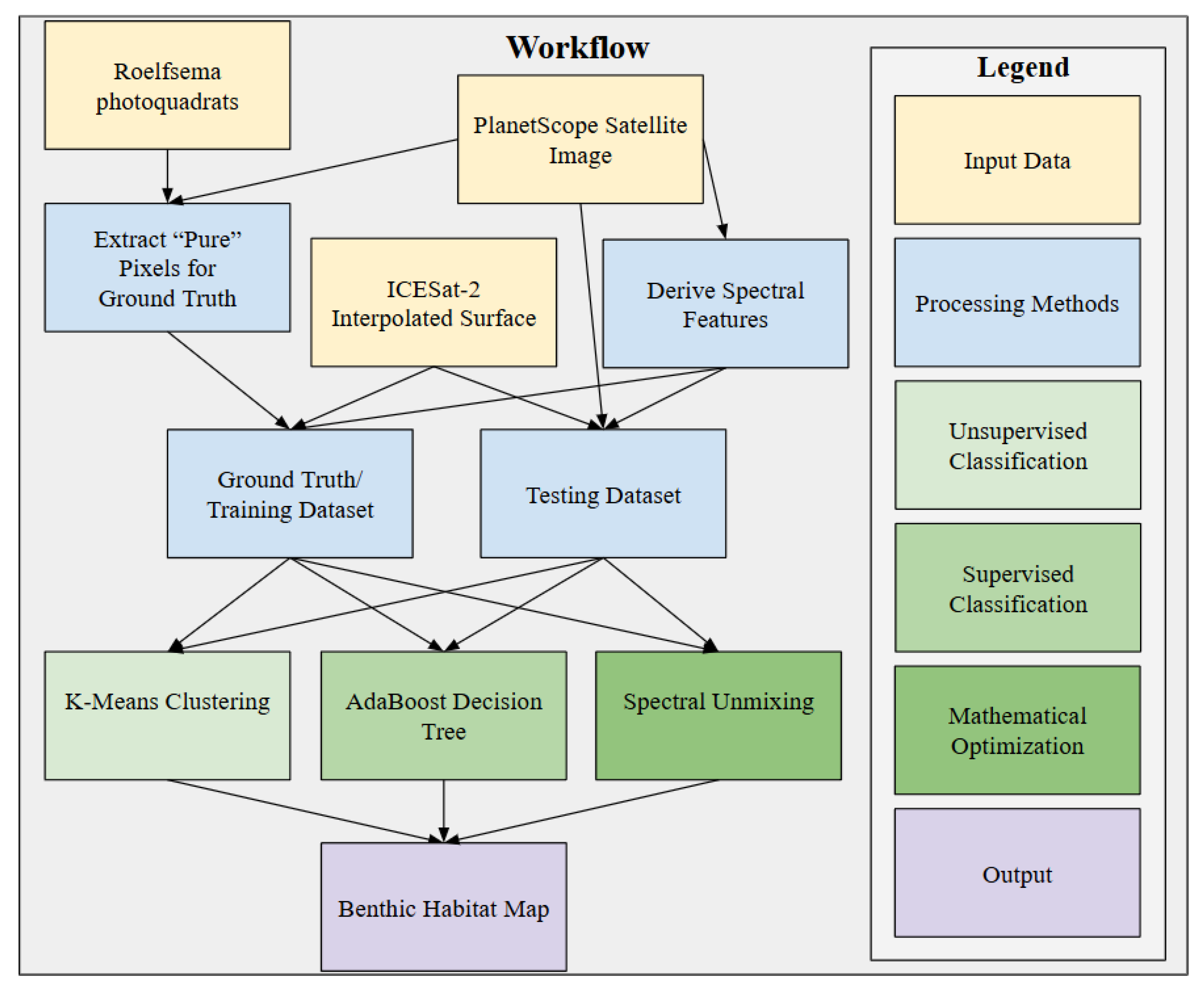
This section describes the machine learning (ML) and mathematical unmixing approaches explored in this article to estimate benthic composition from high-resolution multispectral satellite imagery. The workflow for data processing and methods is shown in Figure 4. The inputs to this workflow included a PlanetScope satellite image, Roelfsema et al. photoquadrats, and an ICESat-2 interpolated surface derived from terrain metrics previously used to classify coral presence [23]. The Roelfsema et al. photoquadrats, spatially aligned with satellite image pixels, were used as a ground truth dataset containing benthic class labels, percent cover for each class within a m area, and associated spectral values. Additional variables were incorporated into both the ground truth dataset and the PlanetScope raster image by deriving spectral features and introducing the ICESat-2 interpolated surface, composed of algorithmically derived terrain metrics. Three modeling approaches (K-Means clustering, AdaBoost decision tree, and mathematical spectral unmixing) were examined to map benthic habitats. These models were trained using the labeled ground truth dataset and then applied to the full processed raster image to generate benthic composition predictions across the study area. The following sections elaborate on each stage of the workflow.

Figure 4.
Project workflow for data processing and data preparation for analysis.
2.6. Ground Truth Processing
To develop a model capable of accurately classifying the benthic composition of the study site, we first constructed a ground truth dataset, which we refer to as the pure pixel library. The performance and reliability of any model, particularly a mathematical one, are inherently limited by the quality of its ground truth data. Accordingly, a comprehensive evaluation of the pure pixel library was conducted to assess the potential difficulty of the classification task.
2.6.1. Constructing the Library of Pure Pixels
Drawing inspiration from the benthic cover classes defined by Phinn et al. [30], a set of relevant and sufficiently broad classes was established and tailored specifically to our study site. In this study, we use the terms benthic class and endmember interchangeably to refer to the dominant biological and physical components of the coral reef: live coral, dead coral, macroalgae, sand, land, and deep water. Each endmember was defined with reference to the Coastal and Marine Ecological Classification Standard (CMECS) [31]. Definitions for each endmember can be found in Table 1.

Table 1.
Definitions of benthic endmember classes, derived from the CMECS.
Each photoquadrat provided by Roelfsema et al. included the percent coverage of each benthic class present in the image. These photoquadrats were approximately m in size, while the raster image derived from PlanetScope had a spatial resolution of 3 m per pixel. To align the scales, we aggregated the photoquadrat data to match the resolution of the satellite imagery. Each PlanetScope pixel contained, on average, one to three photoquadrats. If multiple photoquadrats were present within a pixel, the benthic class that appeared most often was assigned to the pixel; in most cases, all photoquadrats within a pixel belonged to the same class. A pixel was considered “pure” if the aggregated coverage within the corresponding m area contained at least coverage of a single benthic class. This threshold was chosen to enhance spectral separation among classes, and also reflects how spectral unmixing typically relies on in situ spectra collected over patches that are visually homogeneous, though not perfectly uniform. Using , therefore, provides a practical balance between ensuring class purity and retaining enough pixels for analysis. However, one immediate consequence of using a higher threshold was the complete loss of macroalgae representation in the ground truth dataset. Macroalgae are not typically observed in isolation within this environment, growing on or alongside dead coral, making it difficult to isolate within a single m pixel. This spatial mixing introduced considerable challenges in accurately identifying macroalgae at the scale of our analysis. Preliminary classification results confirmed this difficulty, with macroalgae consistently showing highly inconsistent and inaccurate predictions using our available dataset and methods. Given these limitations, we made the decision to exclude macroalgae from further analysis to focus on classes that could be more reliably detected and accurately mapped.
While macroalgae are an ecologically important benthic component, often associated with reef health, their exclusion reflected practical and methodological constraints rather than ecological insignificance. In this case, the decision was driven by the limitations of the available data. Excluding macroalgae represents a trade-off: we forgo some biological specificity in exchange for greater confidence in the accuracy and interpretability of the other mapped classes. Future efforts using higher-resolution imagery or more robust ground truth data may offer a path to incorporating macroalgae more reliably.
The benthic labels in Roelfsema et al.’s dataset were more specific than our broader endmember classes. To align them, we mapped each detailed benthic label to its corresponding endmember. For example, “encrusting Montipora” was categorized as live coral, whereas “bleached encrusting Montipora” was assigned to dead coral. Although bleached corals remain biologically alive, the loss of symbiotic pigments substantially increases their reflectance and reduces spectral contrast, making them optically similar to dead coral, sand, or coral rubble in multispectral imagery [32,33,34]. Because this classification was based on optical rather than physiological differences, bleached encrusting Montipora were grouped with dead coral to reflect this spectral similarity. Roelfsema et al.’s photoquadrats did not include examples of land, and only 11 deep water points were available from their survey. To better incorporate these classes, shapefiles were generated using QGIS (a free and open source GIS software [35]) to delineate regions containing only land or deep water. From each shapefile, a random sample of 300 points was selected to serve as pure pixels for these two endmembers, resulting in 300 points for land and 311 for deep water.
Spectral band values were extracted for each pixel using the PlanetScope satellite image in QGIS. Each pixel was associated with values from the four available spectral bands—red, green, blue, and near-infrared (NIR)—as well as geographic coordinates. Table 2 summarizes the number of pure pixels identified for each benthic class using the coverage threshold.

Table 2.
Number of “pure” pixels identified for each endmember class at a m scale using a coverage threshold. The first four classes (live coral, dead coral, macroalgae, and sand) were derived from Roelfsema et al. [26], while land and deep water were supplemented as described in the text. The source of each class is listed in the rightmost column.
Using these data, two related datasets were constructed:
- The pure pixel library, which contained only the dominant class label for each identified pure pixel. This dataset served as the ground truth for training and evaluating classification models.
- The summary table was organized by unique pixels, with each pixel represented by multiple entries, one for each endmember with non-zero coverage. This format retained the full composition of each pixel, including the majority class as well as all contributing benthic components and their respective percentages.
The pure pixel library and the summary table formed the foundation for the classification methods. Together, these datasets were critical for both the task of classifying benthic composition and the ground-truthing process.
2.6.2. Ground Truth Analysis
Real-world ground truth datasets are often incomplete, noisy, or otherwise imperfect representations of the environment. While ML models offer some flexibility and resilience in learning from noisy or incomplete datasets, mathematical models are inherently constrained by the quality of their inputs. To mitigate the limitations of our ground truth data, we implemented several preprocessing steps, including denoising the data by applying a percent coverage threshold to define “pure” pixels, as well as refining class labels where appropriate. The impact of data imperfections on model performance was evaluated to assess model reliability and motivate the use of supplementary datasets.
To evaluate the quality and reliability of our ground truth data, we conducted a bootstrapped linear unmixing simulation to characterize the uncertainty in the spectral signatures of our endmember classes. For this analysis, we performed 10,000 bootstrap iterations, randomly resampling (with replacement) the dataset in each iteration. Using a least-squares approach, which closely mirrored traditional spectral unmixing methods (see Section Traditional Unmixing Method for more details), we produced a distribution of endmember reflectance values for each spectral band by solving for the relationship between pixel composition and measured reflectance. These statistics provide an averaged spectral signature for each benthic class based on the ground truth data and offer insights into the degree of spectral separability between classes.
To better understand potential sources of classification error in the ground truth data, we investigated the consistency of spectral signatures across benthic class labels. Specifically, we conducted a systematic pairwise comparison of PlanetScope reflectance values across all four bands to identify pixels with identical spectral values. We then examined instances in which these spectrally identical pixels were assigned different benthic class labels. Approximately of ground truth pixels shared duplicate spectral values with at least one other pixel, but were labeled differently. An example is shown in Figure 5, where two pixels with identical spectral values (circled in yellow) are labeled as dead coral (top) and live coral (bottom). These inconsistencies were most frequently observed among live coral, sand, and dead coral classes. This analysis highlights the spectral ambiguity between certain benthic types and underscores the challenge of reliably distinguishing them using spectral data alone.
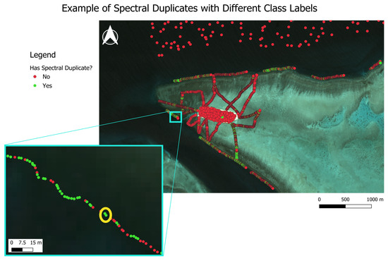
Figure 5.
Two ground truth pixels with identical spectral reflectance values but differing benthic class labels. The pixels, circled in yellow, are labeled as majority dead coral (top) and majority live coral (bottom).
In order to quantify the extent of this spectral ambiguity and assess whether reflectance values provide a reliable basis for distinguishing classes, we conducted formal statistical tests to more formally assess the separability of classes in spectral space. Specifically, we conducted Kruskal–Wallis tests followed by post hoc Steel–Dwass comparisons to determine whether reflectance values differed significantly among benthic classes and to identify which class pairs were distinguishable.
The Kruskal–Wallis test, a nonparametric alternative to one-way ANOVA, was appropriate given that the reflectance distributions violated normality assumptions. This test, implemented in JMP Pro (version 18; [36]), evaluates the null hypothesis that all group medians are equal. Reflectance values for each spectral band were entered as response variables, and benthic class labels served as grouping factors. JMP ranks all observations across groups, computes the mean rank per group, and then calculates the test statistic:
where k is the number of groups (i.e., benthic classes), is the number of observations in group i, N is the total sample size, is the mean rank for group i, and is the overall mean rank. This formula assumes no tied ranks; JMP automatically applies a tie correction factor according to standard Kruskal–Wallis procedures. A significant test result (p-value < 0.05) indicates that at least one class differs from the others.
Following the Kruskal–Wallis tests, we applied the Steel–Dwass procedure to identify which pairs of benthic classes differed significantly in their spectral reflectance distributions. The Steel–Dwass procedure, which supports nonparametric pairwise comparisons, was chosen over other post hoc options because it allows all-pair comparisons in a fully nonparametric framework while controlling for multiple testing, making it particularly appropriate for our data. This post hoc test, implemented in JMP Pro (version 18; [36]), performs all possible pairwise comparisons between groups using rank-based differences. For each pair of classes i and j, JMP computes the test statistic as follows:
where and are the mean ranks for classes i and j, and are the number of observations in each class, and N is the total number of samples. JMP compares each statistic and summarizes the results using grouping letters to indicate statistically homogeneous subsets of classes. Classes that share the same letter are not significantly different from each other, whereas classes with different letters differ significantly.
Both the Kruskal–Wallis and Steel–Dwass tests were conducted using reflectance values from all ground truth pixels in the pure pixel library, providing a quantitative framework for evaluating how reliably spectral data alone can distinguish benthic classes. Together, these tests form a robust nonparametric approach to assess spectral separability among benthic types.
Our analysis revealed important limitations of relying solely on spectral data. The presence of pixels with identical spectral signatures but differing class labels (particularly among live coral, dead coral, and sand) demonstrated the extent of spectral overlap between some benthic types. This ambiguity underscores the difficulty in achieving accurate classification using reflectance data alone, highlighting the importance of exploring additional datasets to support more robust benthic mapping.
2.7. Feature Engineering
Based on our analysis of the ground truth data, it became clear that expanding the set of input variables was necessary to improve classification performance. While the pure pixel library—composed of four spectral bands and the percent cover of each benthic class—served as the foundation of the ground truth dataset, we expanded this dataset with additional variables that were both extractable from available data sources and potentially informative for distinguishing benthic habitats. These same variables were incorporated into the raster image used for model training and testing. First, we derived additional spectral features directly from the original spectral bands. Second, we incorporated terrain-specific parameters (rugosity, slope, and depth) from the ICESat-2 surface generated for the study site. As shown in our ground truth data analysis, duplicate spectral values with conflicting class labels and substantial class overlap in some bands indicated that spectral data alone might be insufficient for reliable classification of benthic classes. Therefore, the inclusion of ecologically relevant parameters was a necessary step toward improving model performance. The following sections detail the derivation of these parameters, and their relationship to benthic classes is presented in Section 3.
2.7.1. Derived Spectral Features
To enrich the input data and enhance the separability of benthic classes, we extracted additional spectral features from the original four PlanetScope bands (blue, green, red, and NIR). Drawing inspiration from traditional spectral indices used in remote sensing, such as the Normalized Difference Vegetation Index (NDVI) [37] and the Normalized Difference Moisture Index (NDMI) [38], we computed band ratios and differences between standardized bands (i.e., standardized to z-scores). These derived parameters were intended to highlight subtle spectral variations and amplify class-specific signals that may not be easily distinguishable using raw reflectance values alone. For instance, NDVI enhances vegetation signals by leveraging the high reflectance of healthy vegetation in the NIR band relative to the red band [39], and our aim was to achieve similar improvements in class discrimination with the band ratios and scaled band differences.
We calculated band ratios for all unique two-band combinations, excluding inversions and self-pairs. For a given pixel i, the ratio of band 1 to band 2 was computed as follows:
We also computed differences of standardized bands. To reduce the influence of band-specific magnitude scales, each band was first standardized by subtracting its mean and dividing by its standard deviation across the dataset. The difference between the standardized band 1 and band 2 for pixel i was given by
Both band ratios and differences were appended to each pixel in the pure pixel library and the raster dataset. By including these 12 additional features alongside the original spectral bands, we aimed to maximize the information available to our classification models and improve their ability to distinguish between benthic endmembers.
2.7.2. ICESat-2 Interpolated Surface
In our previous work [23], ICESat-2 tracks were used to derive several parameters aimed at identifying areas of the study site containing corals. Key parameters included rugosity, slope, and the median depth of ICESat-2 photon events (PEs) algorithmically classified as bathymetry, and satellite-derived bathymetry (SDB) from the Allen Coral Atlas (ACA) [40]. In [23], these variables were used in ML models to create a binary ‘reef’/‘no reef’ predictor, which was incorporated as a parameter in this work. All variables were then interpolated using Voronoi polygons to generate a continuous surface covering the entire study area. To implement these data in this work, we used QGIS to extract data from this surface in a grid format matching the spatial resolution of the 3 m raster of the satellite imagery.
The ICESat-2 data were incorporated into both the pure pixel library (ground truth dataset) and the raster data from the satellite image, which served as the training and testing datasets, respectively. Therefore, the training and testing datasets contained spectral data from the satellite imagery, derived spectral features including band differences and ratios, and ICESat-2-extracted parameters.
2.8. Classification Methods
Using the PlanetScope multispectral satellite image and the pure pixel library, we classified the benthic habitat composition of Heron Reef. To achieve this, we applied unsupervised, semi-supervised, and supervised ML classification methods, namely K-Means clustering and AdaBoost decision trees, as well as an optimization-based spectral unmixing method. These approaches were selected to provide a baseline comparison across unsupervised (K-Means), supervised (AdaBoost), and mathematically motivated methods, while remaining simple and interpretable. Traditional linear spectral unmixing was not included because the incorporation of ICESat-2-derived features (e.g., depth, slope, rugosity) violates its spectral-only assumptions. This setup allows us to evaluate the contribution of both spectral and ancillary spatial data.
The inputs to these models included the four original spectral bands (red, green, blue, and NIR), 12 derived spectral features, and five features from the ICESat-2 interpolated surface (Table 3).

Table 3.
Summary of input features used for benthic habitat classification, including original spectral bands, derived spectral features, and ICESat-2 interpolated surface metrics.
Though these methods produced pixel-based classifications, the nature of their outputs reflected a fundamental difference in assumptions between the ML methods and the mathematical unmixing approach. Both K-Means clustering and AdaBoost decision trees generate a probability for each class within a pixel, and then typically assign the pixel to the class with the highest probability. In these methods, the underlying assumption was that each pixel truly belongs to a single class, and the probabilities simply reflect uncertainty about which class that is. K-Means does this by grouping observations based on their similarity to cluster centers, while AdaBoost combines multiple decision trees to produce class probabilities. In contrast, spectral unmixing offers a more ecologically realistic output by assuming that multiple classes can coexist within a pixel and estimates the fractional cover of each. This sub-pixel information was particularly valuable for benthic habitat mapping, where mixed substrate types are common and ecologically important. Although we converted the unmixing results into discrete maps for comparison with the ML classifications, the continuous abundance maps produced by unmixing have the potential to better capture the true complexity of benthic composition.
To assess the added value of ICESat-2 data and the strength of the PlanetScope satellite image on its own, we compared model performance between two sets of inputs: (1) satellite imagery and derived spectral features and (2) satellite imagery and spectral features combined with ICESat-2-derived parameters. Models were trained on the ground truth pure pixel library (1064 pixels) and applied to the remaining pixels of the satellite image raster (8,069,329 pixels). Pixels used in the training set were excluded from the testing set to ensure independent evaluation. The following sections define each classification method.
2.8.1. Unsupervised and Semi-Supervised: K-Means Clustering
K-Means clustering is an unsupervised ML algorithm that partitions a dataset into K clusters based on their feature-space similarity [41]. The algorithm randomly initializes cluster centers and iteratively refines them so that points within a cluster are more similar to each other than to those in other clusters—i.e., it minimizes within-cluster variance while maximizing between-cluster variance for a user-specified number of clusters. K-Means produces hard classifications, assigning each pixel to exactly one class based on its proximity to the nearest cluster center.
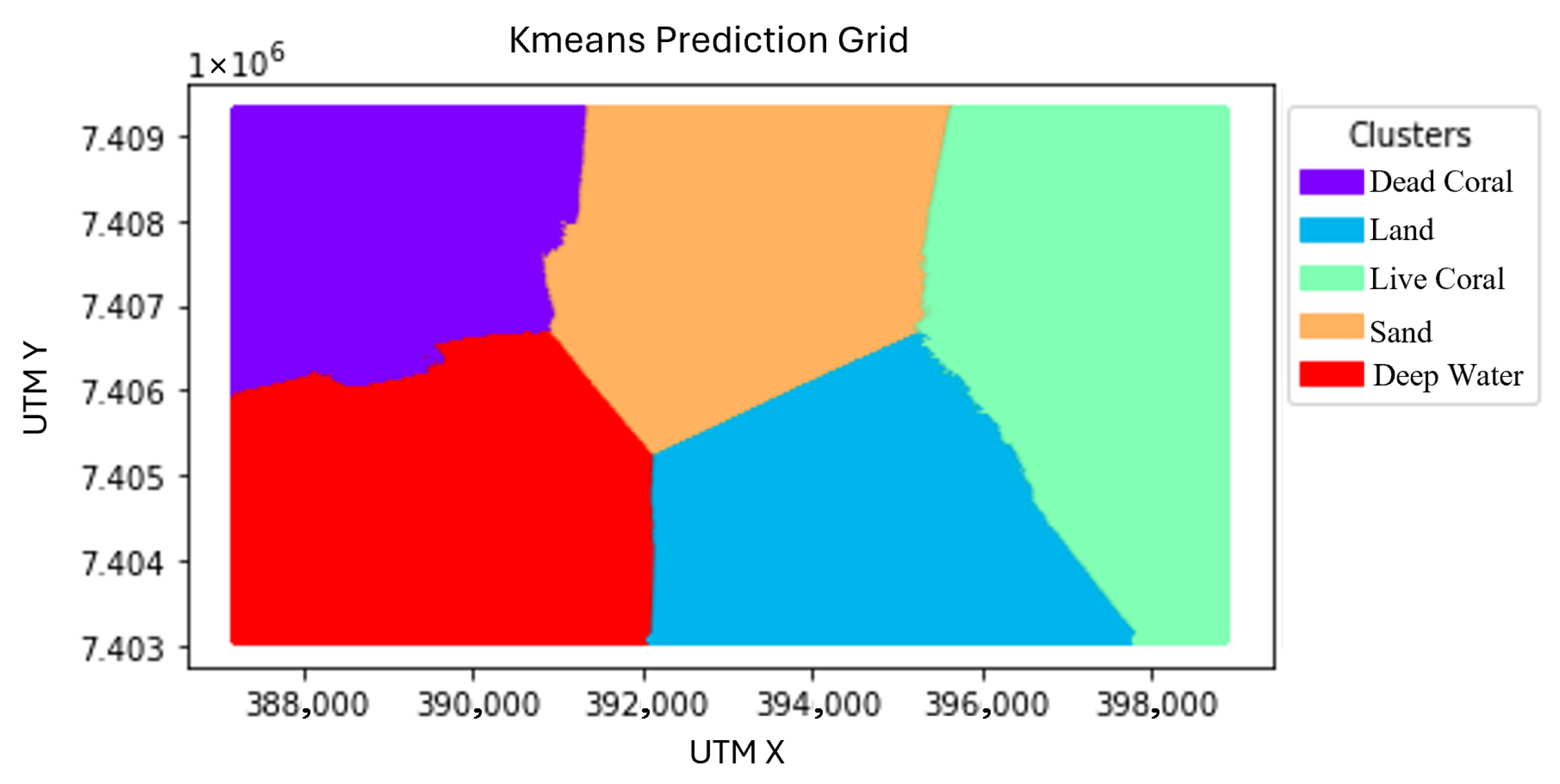
An unsupervised implementation of K-Means was initially tested on the satellite imagery, where the algorithm was applied without any prior knowledge of the underlying classes. However, this approach resulted in poor classification performance, as the algorithm tended to divide the geographical region into K spatially uniform clusters rather than distinguishing meaningful spectral differences between coral reef features (Figure 6).
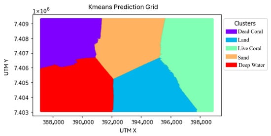
Figure 6.
Unsupervised K-Means clustering results. Map is displayed in UTM coordinates, Zone 56S. The satellite image in Figure 2 serves as a reference.
These limitations led us to implement a semi-supervised variation of K-Means, where cluster initialization was guided by prior knowledge. Instead of randomly initializing cluster centers, we leveraged our pure pixel library, containing ground truth examples for each benthic class. Cluster centers were randomly selected from this library for each class, ensuring that each cluster was initialized with a meaningful representative spectrum. The number of clusters was fixed at five, corresponding to the number of benthic habitat classes. The model was then applied to the entire study area after being trained on the selected centers, producing a categorical map where each pixel was assigned to one of the five benthic classes.
The semi-supervised initialization significantly improved classification results compared to the fully unsupervised approach, as it ensured that the initial cluster centers were relevant to the spectral diversity present in the dataset. This method was run in two iterations: (1) satellite imagery and derived spectral features and (2) satellite imagery, spectral features, and ICESat-2-derived parameters. This approach allowed us to evaluate the effectiveness of classification based solely on satellite-derived data and to assess whether the addition of ICESat-2 parameters improves model performance.
2.8.2. Supervised: Adaboost Decision Tree
Decision trees are a supervised ML algorithm that use a tree-like model to split data into branches designed to separate the data in a way that maximizes class distinction. Although decision trees can capture complex patterns in the training data, their ability to detect and model relatively minor trends makes them prone to overfitting.
Adaptive Boosting (AdaBoost) algorithms are a method of ensemble learning that improves the accuracy of decision trees by iteratively learning from the mistakes made. AdaBoost algorithms create a sequence of weighted decision trees, which adapt based on the errors of the previous trees, giving more weight to previously misclassified examples [42]. This process gradually improves overall accuracy by combining the strengths of many weak models. Unlike K-Means, AdaBoost decision trees generate probability distributions for each class per pixel, and ultimately assign each pixel to the single class with the highest probability.
We trained the AdaBoost decision tree model on the library of pure pixels (the ground truth data), and tested it on the remainder of the satellite raster image. Consistent with the K-Means clustering method, we tested two input configurations to assess how ICESat-2-derived parameters improve model accuracy. Both the testing and training datasets were scaled using Python’s (version 3.10.14) StandardScaler [43]. Hyperparameters for this model, including the number of estimators and learning rate, were selected using a grid search method that optimizes accuracy. Ultimately, 70 estimators and a learning rate of were used. The final output was a categorical map in which each pixel received a single class assignment based on the highest probability prediction.
We also measured feature importance to gain an understanding of which variables most strongly influenced the model’s ability to correctly classify benthic composition. Feature importance was calculated as the Gini importance, which quantifies the contribution of each feature in reducing impurity within the model [44]; higher scores indicated greater importance.
2.8.3. Spectral Unmixing Methods
Our approach to spectral unmixing is based on the traditional formulation, in which each pixel is modeled as a mixture of multiple benthic classes, or “endmembers.” Unlike the ML methods that assign each pixel to a single class, spectral unmixing provides the percent coverage of every endmember class within each pixel, offering a more comprehensive representation of benthic composition. This section is structured in three parts. First, we review the standard linear unmixing approach. Next, we introduce a preliminary inversion-based method that reverses this process. This preliminary analysis served as an exploratory tool to assess the informativeness of each input feature. Finally, we describe our primary modeling framework—a two-part, nonlinear formulation—that incorporated insights from the preliminary analysis to improve performance.
Traditional Unmixing Method
In traditional spectral unmixing, each pixel in a raster image is assumed to be a linear combination of endmembers (pure spectral components) and their associated abundances. In this study, we use the terms abundances and percent cover interchangeably, following common practice in the literature where both refer to the fractional contribution of a benthic class to a pixel [45,46,47]. The 1-D model for a single pixel is as follows:
where
- is the abundance (fractional contribution) of endmember m;
- is the spectral signature of endmember m;
- e is an error term for all possible sources of error (i.e., sensor sensitivity, location accuracy, etc.);
- M is the number of endmembers (typically number of spectral bands);
- N is the number of pixels.
Assume that the abundances for endmember m have the following properties:
- Additivity:
- Non-negativity: for
- Bounds: for
This problem can be generalized to a 2-D raster X (pixels × bands), giving the matrix formulation
where
- is the raster image (with N pixels and B spectral bands);
- is the spectral library (with M endmembers);
- is the abundance matrix;
- E is the residual error.
Traditionally, the spectral library S is produced by in situ measurements or derived from known reference spectra, while X is observed from satellite imagery. The unmixing objective is then formulated as an optimization problem, where the goal is to solve for A by minimizing the squared error between the reconstructed and measured X. Let the satellite image X have width W and height H, such that pixels are denoted by spatial indices with and , and endmembers are indexed by . The least squares formulation is then
subject to
Solving this optimization problem yields the abundance matrix A, which contains the estimated fractional coverages of each endmember class for every pixel in the raster image. Each column of A corresponds to a pixel and each row to a class (e.g., live coral, sand, etc.), with values representing the percentage of that pixel’s area covered by the corresponding class. The additivity constraint ensures that the total coverage across all classes sums to for each pixel. As such, the model’s output provides a spatially explicit, per-pixel map of benthic composition where each pixel contains abundance information for all endmember classes.
Preliminary Feature Analysis on the Simple Method
To identify which input features are most informative for distinguishing benthic classes, we first conducted a preliminary analysis using a simplified inversion of the traditional spectral unmixing formulation. Rather than using a known spectral library to estimate abundances, we used a labeled ground truth dataset (the pure pixel library) that contains measured percent cover values for each pixel, which we treat as abundances to align with the spectral unmixing framework. These abundances, , paired with corresponding satellite pixels, , served as training data to estimate a scene-specific spectral library . Note that contains only values derived from ground truth data, including the original four spectral bands, derived spectral features, and ICESat-2 interpolated surface features. Subsequent references to x without the subscript “” refer to the remaining pixels in the test dataset. We will refer to the inputs as features rather than spectral bands.
The new objective function was derived from the traditional problem formulation by applying the singular value decomposition (SVD) to , where
This was substituted into the original problem as follows:
where is the pseudoinverse of the spectral library, defined as
This reformulation was also posed as an optimization problem to solve for by minimizing the squared error, yielding a least squares solution:
Although lacks direct physical interpretation as a spectral library (i.e., its columns do not represent real material spectra), its structure provided insight into the contribution of each input variable to the detection of individual classes. Each column of corresponds to a single endmember class (e.g., live coral, dead coral, sand, etc.), while each row represents a specific input variable. To quantify variable importance, we computed matrix norms of in two complementary ways.
First, we assessed the overall contribution of each variable across all classes using the column-wise -norm:
This norm provided a global measure of how much each variable influences the model across all endmembers.
Second, we computed the row-wise -norm to evaluate the strongest class-specific influence of each variable:
This highlighted the variable(s) with the strongest influence on each class, identifying which features were most predictive of a given benthic type. Together, these norms provided an interpretable summary of how each feature contributes to the classification of individual benthic types and overall model performance.
This preliminary inversion-based analysis was not used for final classification; instead, it served to guide variable selection for our primary modeling approach. Feature importance results are shown in Figure 7 and Figure 8. In both analyses, only the spectral bands and their derived features proved to be substantially impactful. Therefore, ICESat-2-derived parameters were excluded from the unmixing method in subsequent steps.

Figure 7.
Global (column-wise) feature importance for the unmixing model.
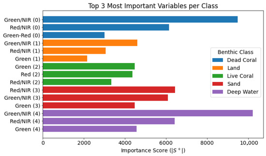
Figure 8.
Row-wise feature importance for the unmixing model by class.
Novel Unmixing Method
Our novel unmixing method builds on the traditional linear mixing model by incorporating a two-part nonlinear optimization strategy. First, we estimated spectral signatures (S) using ground truth pixels, and then used the estimated S to solve for pixel abundances (A).
- Estimating Spectral Signatures (S):
We estimated the matrix of spectral signatures, S, as a weighted mean of the ground truth pixel spectra. Using the definition of a weighted mean, we define S as follows:
where
- is the spectral library (with M endmembers and B features);
- contains the abundance values for each ground truth pixel (with N pixels);
- is the matrix of corresponding satellite spectra for the ground truth pixels.
We solved for S as a linear system by reformulating the problem as follows:
which can be solved using least squares:
- Estimating Pixel Abundances (A):
In remote sensing, band ratioing is a technique used to enhance information obtained from spectral bands and refine spectral variations through the division of two bands [48]. Incorporating this concept of band ratios into spectral unmixing, we reformulated the unmixing problem nonlinearly. We defined the nonlinear objective function as follows:
where
- is the abundance vector for a given pixel;
- contains the input features for that pixel;
- is the estimated spectral library;
- B is the number of input features;
- M is the number of endmembers.
We maintained the same assumptions of full additivity, non-negativity, and purity as the linear mixed model, and imposed these constraints. We then minimized the objective function with respect to A, using the Sequential Least Squares Programming method in Python’s (version 3.10.14) SciPy.optimize package.
As described in the traditional unmixing method, the output of the unmixing model was the abundance matrix A, which represents the percent coverage of each endmember class per pixel. For clarity in the analysis, we hereafter refer to these values as percent cover. This fundamental difference in output (i.e., providing continuous percent cover values rather than discrete class assignments) distinguishes unmixing from the ML approaches. To facilitate comparison with the results of our ML models, we also presented the class corresponding to the most dominant endmember for each pixel. While this classification summary aided in consistency across methods, the full percent cover vectors might offer a more nuanced and accurate representation of mixed benthic cover. As such, we considered both the most dominant class and the full percent cover estimates in our analysis.
2.8.4. Benthic Coverage Estimation Method
To estimate benthic class coverage across the Heron Reef study area, we used the full-pixel prediction maps generated by each classification method. For each model, we computed the total number of pixels assigned to each benthic class and expressed this as a proportion of the total area. We selected the best-performing model for each method based on validation accuracy using the ground truth pure pixel library, and subsequently applied it to the remaining pixels of the satellite image to generate full-coverage classification maps that reflect the optimal performance of each method. For the unmixing method, we compare the benthic coverage produced by the most dominant endmember of each pixel and the sub-pixel percent cover maps.
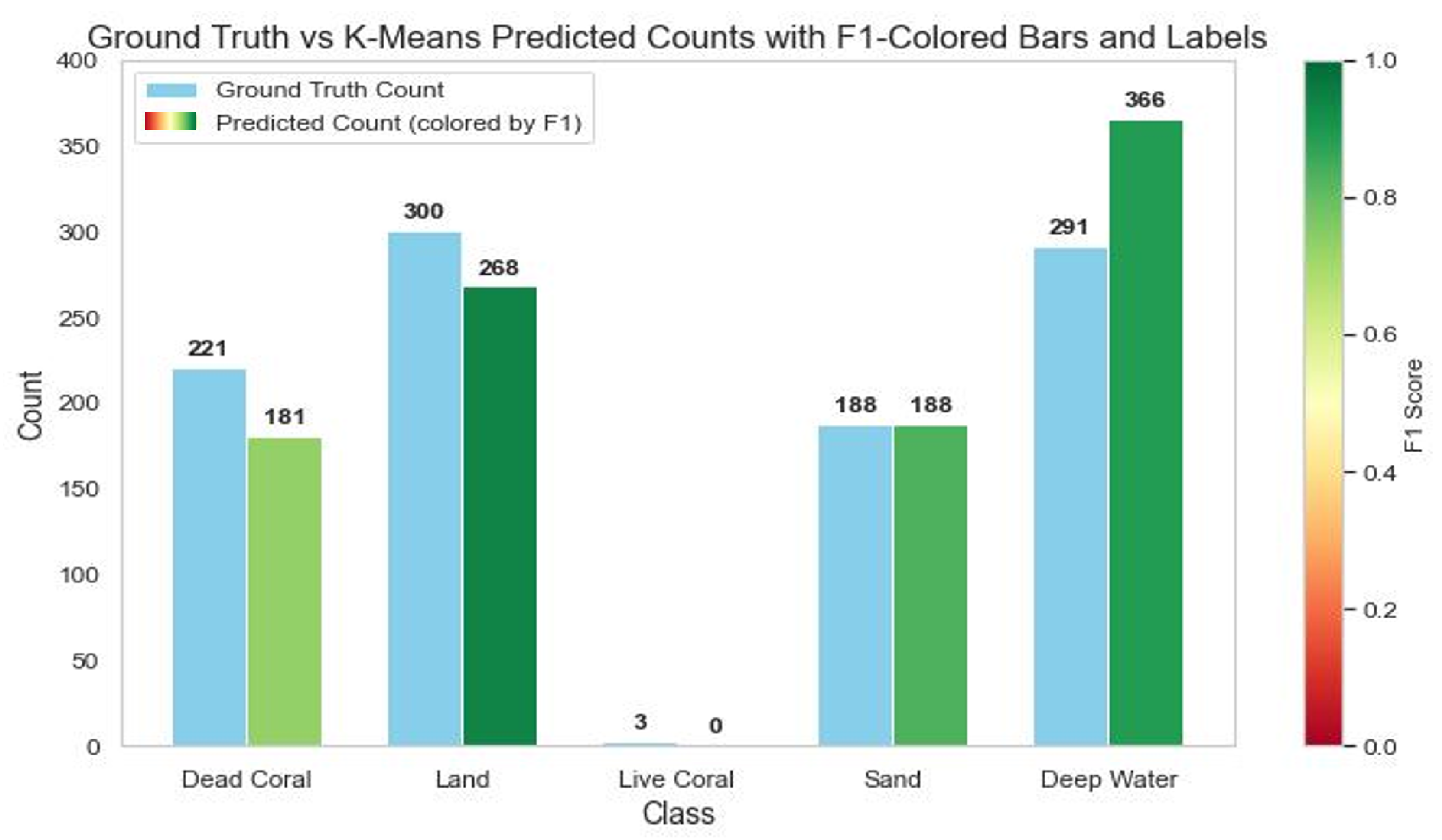
These raw coverage proportions provided a model-driven estimate of benthic composition, but they do not account for the quality of the model’s predictions. Moreover, our ground truth dataset represented only approximately of the study site. To address these limitations, we incorporated performance metrics to validate results with the ground truth dataset. Specifically, we examined both the confusion matrices and class-based F1 scores on the validation data to assess how well each class was predicted. For example, if the ground truth set includes 221 dead coral pixels and the model correctly predicts 181 of them, resulting in an F1 score of , this would indicate a relatively reliable model. To aid in interpretation, we color-coded the predicted pixel counts by class-level F1 scores using thresholds commonly applied in the literature: high (F1 > 0.7), medium (0.5–0.7), and low (<0.5) [49]. By comparing the number of ground truth and predicted pixels per class, we assessed not only overall classification accuracy but also potential biases—i.e, whether it tends to over- or underpredict certain classes.
3. Results
3.1. Class Separability in Spectral Bands
Understanding how well spectral reflectance alone can distinguish among benthic classes is essential for evaluating the limitations of our classification approaches. To evaluate spectral separability, we first performed a bootstrapped linear unmixing simulation. We then conducted Kruskal–Wallis tests followed by Steel–Dwass post hoc comparisons to evaluate whether significant differences in reflectance exist among classes in each spectral band.
The bootstrapped unmixing simulation produced distinct spectral patterns across classes, revealing the strongest contrast observed between land and deep water (Figure 9). Live coral, dead coral, and sand exhibited broadly similar spectral shapes with modest differences in magnitude, particularly in the red, blue, and green bands, where dead coral tended to be slightly brighter than the other benthic classes. This pattern arises from our classification of bleached coral as dead coral, which generally has high reflectance [50], while sand pixels in the study area appear darker in the figure due to averaging and potential water column effects or shading. The NIR band returned low values across all classes, with only slightly higher reflectance for land, as expected given the minimal NIR signal from submerged surfaces. Overall, these results indicate that the classes are most distinguishable in the red, green, and blue bands, while the subtle spectral separation among benthic classes suggests that reflectance alone may be insufficient for reliable discrimination, underscoring the need for additional structural or contextual information.
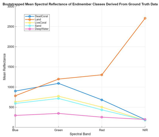
Figure 9.
Bootstrapped mean spectral reflectance of endmember classes derived from ground truth data, showing average reflectance values for blue, green, red, and NIR spectral bands.
The Kruskal–Wallis test results (Table 4) indicated that the median reflectance differed among at least some benthic classes in all spectral bands (blue, green, red, and NIR), with all tests yielding . Subsequent pairwise comparisons using the Steel–Dwass test identified which specific class medians differed significantly within each band. This indicates that each feature contributes some degree of meaningful information for distinguishing benthic types. Larger Chi-square values reflect stronger separation in the ranked reflectance values, suggesting more pronounced class differences.

Table 4.
Summary of Kruskal–Wallis tests and Steel–Dwass post hoc comparisons for each spectral band. Groupings are based on connecting letter reports; classes not sharing a letter differ significantly.
However, the Steel–Dwass post hoc comparisons revealed persistent spectral confusion among several classes. Notably, live coral and deep water were not significantly different in the blue, green, and red bands, and in the NIR band, only land was clearly separated from all other classes. These results confirm that, although statistical differences exist overall, spectral overlap among classes remains a major challenge.
These findings reinforce that spectral data alone are insufficient for reliable benthic classification. Despite preprocessing steps to enhance class separability, the reflectance similarity between classes, such as live coral, dead coral, and deep water, limits classification accuracy. These results strongly support the need to incorporate additional datasets to improve class discrimination and model performance.
3.2. Classification Results
The results of the classification models were evaluated based on their ability to predict the benthic composition of the ground truth data. Recall that the ground truth dataset consisted of labeled pixels from photoquadrat surveys, each matched with corresponding spectral and ICESat-2 measurements. Model performance was assessed both quantitatively, based on predictions for the ground truth pixels, and qualitatively, by examining the resulting benthic composition maps produced using the test data. Performance metrics included overall (global) accuracy and class-specific F1 scores. Class-specific F1 scores balance precision and recall for each class, providing a more informative measure of classification accuracy for each class. This metric is especially valuable when class distributions are uneven, as it is less sensitive to imbalance than overall accuracy.
To facilitate direct comparison, Table 5 summarizes the overall accuracies and class-based F1 scores for all classification models under both input configurations: (1) spectral reflectance and derived spectral features and (2) spectral reflectance, derived spectral features, and ICESat-2-derived parameters.

Table 5.
Summary of model performance, expressed as overall accuracy and class-based F1 scores, for all tested models and input configurations. Input configurations are (1) spectral reflectance and derived spectral features, and (2) spectral reflectance, derived spectral features, and ICESat-2-derived parameters.
3.2.1. K-Means Clustering
This section presents the classification results of the K-Means clustering models and highlights how different input combinations affect overall and class-specific performance.
Figure 10 shows the resulting benthic habitat maps. The left displays results from the model trained with spectral data and derived spectral features (input configuration 1), which achieved an overall accuracy of relative to the ground truth dataset.

Figure 10.
(Left): Semi-supervised K-Means clustering trained using spectral data and derived spectral features. (Right): Model including spectral data, derived spectral features, and ICESat-2 derived data. Both maps are displayed in UTM coordinates, Zone 56S. The satellite image in Figure 2 serves as a reference.
In comparison, the right image in Figure 10 presents the results of the model trained using the second input configuration, which included all possible data: spectral reflectance, derived spectral features, and ICESat-2-derived parameters. The inclusion of the ICESat-2 data resulted in a lower overall accuracy of . The decline in performance may be due to ICESat-2 features (e.g., depth, slope, and rugosity) introducing noise or emphasizing patterns not well aligned with the spectral patterns that separate habitat classes, disrupting the clustering structure. For reference, the interpolated ICESat-2 surfaces are provided in Appendix A, which illustrate the spatial distribution of these features across the study area.
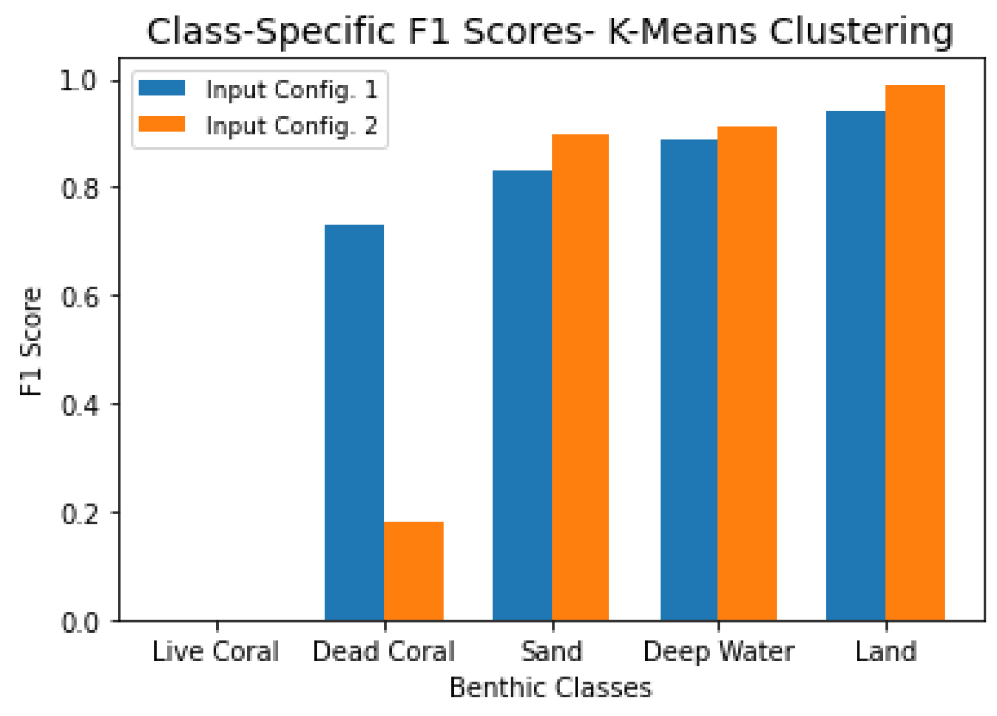
Although the first model produced higher overall accuracy and visually cleaner benthic maps, class-specific performance provides a more nuanced picture. Figure 11 compares the F1 scores by class for both models. The model without ICESat-2 data performed substantially better in identifying dead coral, which explains its higher overall accuracy. However, the model with ICESat-2 data performed slightly better in classifying sand, deep water, and land.

Figure 11.
Class-specific F1 scores for the K-Means clustering model trained (1) satellite imagery and derived spectral features and (2) satellite imagery, spectral features, and ICESat-2-derived parameters.
Overall, the model trained on spectral-only data offers a more balanced performance across all habitat classes (Figure 11), making it the more robust and reliable of the two. Based on both overall accuracy and class-specific F1 scores, we conclude that the K-Means clustering model trained only on spectral data and derived features is the preferred input configuration for this semi-supervised classification approach.
3.2.2. AdaBoost Decision Tree
This section summarizes the performance of AdaBoost decision tree models under two input configurations and examines the influences of input choice on classification accuracy, class-level performance, and feature importance.
Figure 12 shows the resulting benthic habitat maps. The left displays results from the model trained with spectral data and derived spectral features (input configuration 1), which achieved an overall accuracy of relative to the ground truth dataset. In comparison, the right image in Figure 12 presents the results of the model trained using the second input configuration, which included all possible data: spectral reflectance, derived spectral features, and ICESat-2-derived parameters. This expanded input set led to a slightly decreased accuracy of .

Figure 12.
(Left): AdaBoost model trained on spectral bands and derived spectral features. (Right): AdaBoost model trained using all possible data: spectral data, derived spectral features, and ICESat-2 derived data. Both maps are displayed in UTM coordinates, Zone 56S. The satellite image in Figure 2 serves as a reference.
Feature importance for the model trained on input configuration 1 is shown in Figure 13. The most influential predictors were the NIR, green, and blue–red bands, and they were significantly more impactful than any of the other features. In contrast, features such as the blue–NIR and blue/green bands had no measurable contribution. The remaining features contributed only minor improvements to overall classification performance.
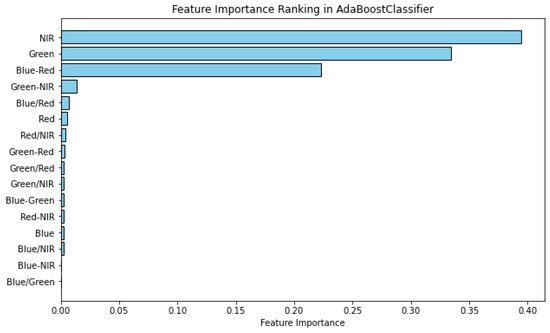
Figure 13.
Relative feature importance for the AdaBoost model trained on spectral bands and derived spectral features.
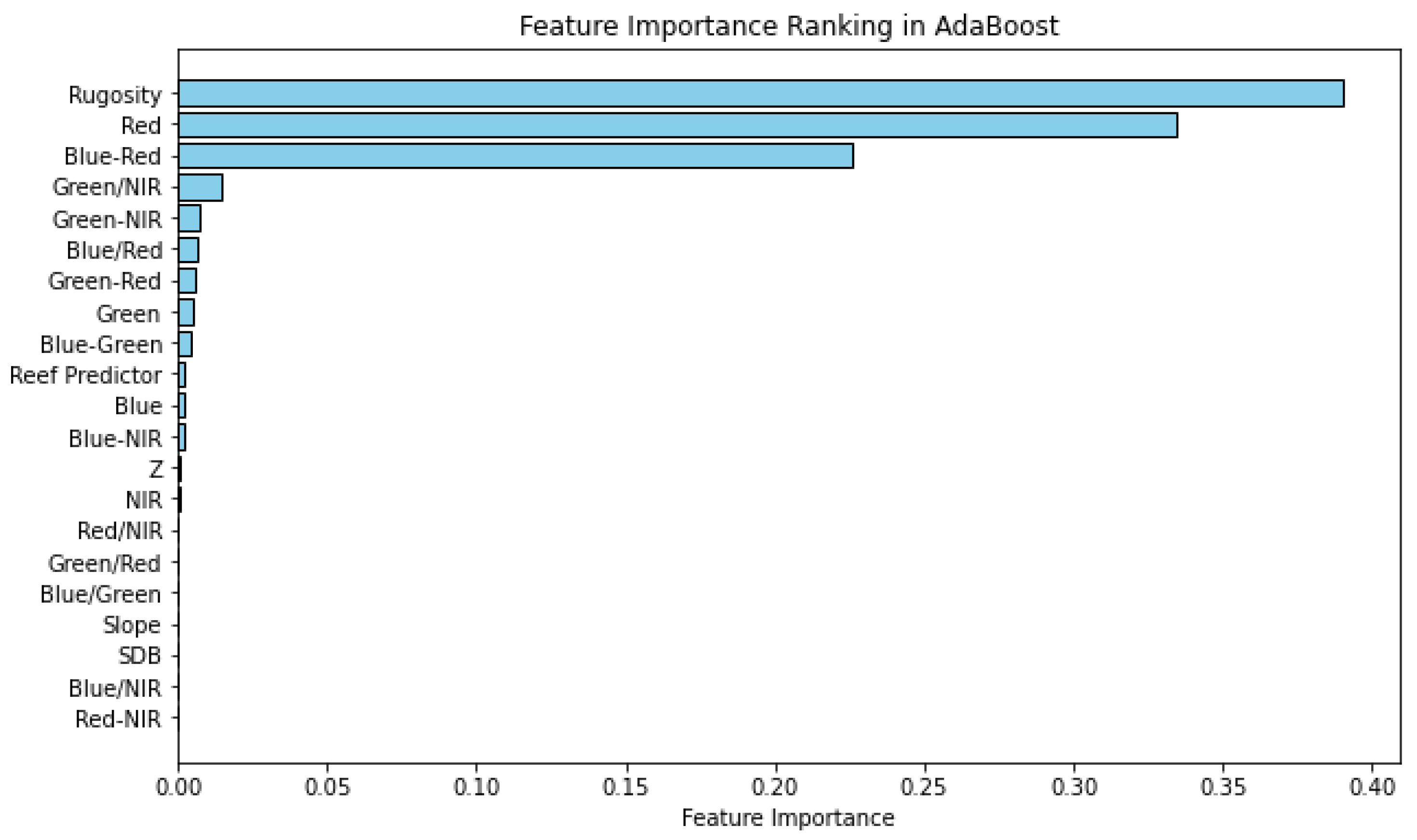
Feature importance analysis for the model trained on input configuration 2 (Figure 14) revealed a shift in the most impactful predictors. The top predictors were rugosity, red band, and blue–red bands, suggesting that the geophysical information derived from ICESat-2 played a key role in boosting model performance. The previous top-ranked spectral features (such as the NIR, green, and blue–red bands) were much less impactful in this model. Additionally, features such as the red/NIR bands, green/red bands, blue/green bands, slope, SDB, blue/NIR bands, and red/NIR bands made no measurable contribution. The remaining features contributed only minor improvements to overall classification performance.

Figure 14.
Relative feature importance for the AdaBoost model trained using all possible data: spectral data, derived spectral features, and ICESat-2 derived data.
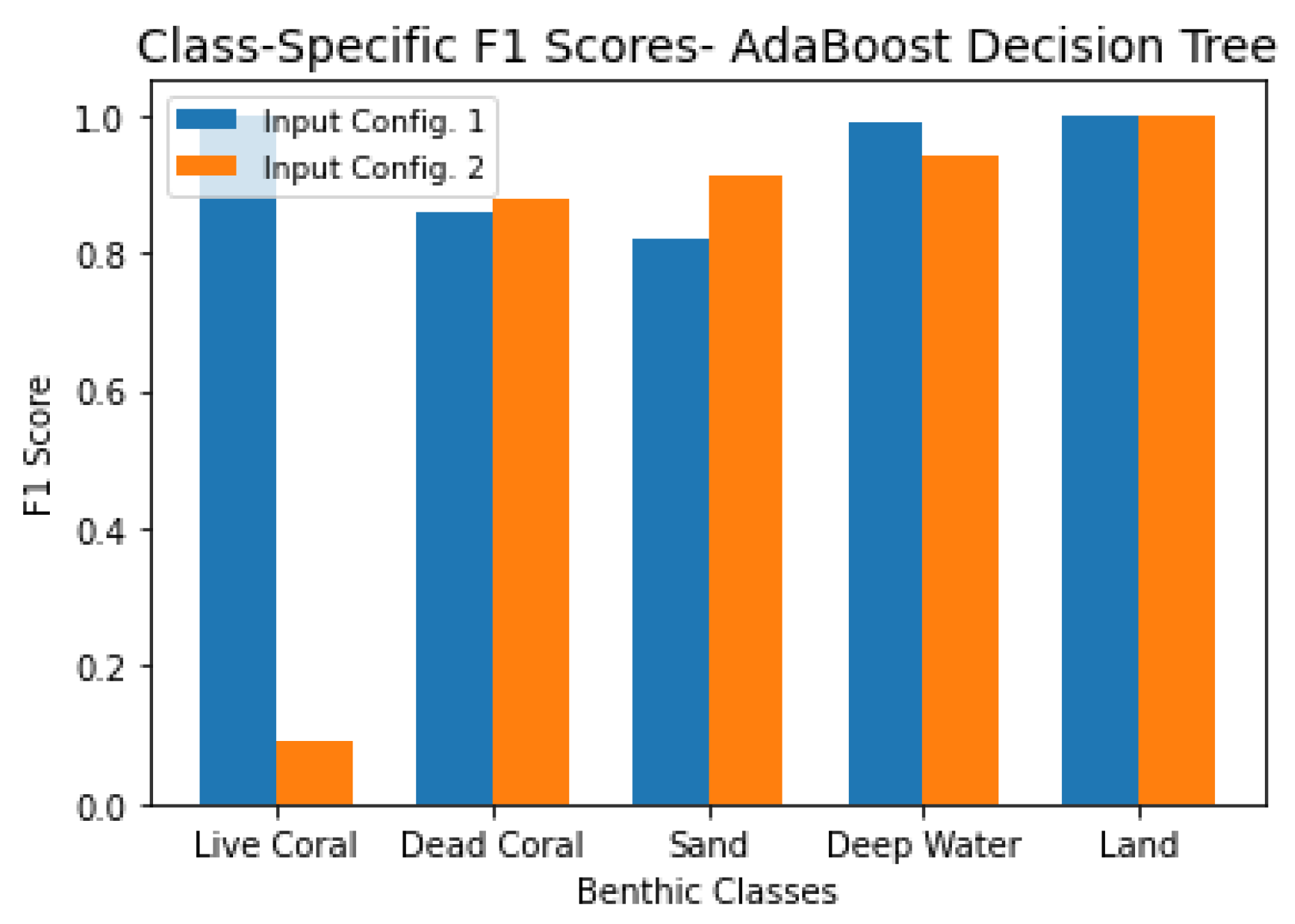
Overall, the first model achieved only slightly higher overall accuracy () compared with the second model (). As shown in Figure 15, which compares F1 scores by class, the first model performed marginally better in identifying live coral, while the second model, which incorporated ICESat-2 data, showed small improvements in classifying the other benthic classes.

Figure 15.
Class-specific F1 scores for the AdaBoost decision tree model trained (1) satellite imagery and derived spectral features, and (2) satellite imagery, spectral features, and ICESat-2- derived parameters.
These results indicate that, although the inclusion of ICESat-2-derived parameters in the AdaBoost model did not improve overall accuracy ( vs. for the spectral-only model), it provided small gains in classifying most benthic classes. The spectral-only model, on the other hand, performed much better in identifying live coral, consistent with previous work showing that this region is known to be coral-rich [51,52]. As shown in Figure 12, the first model also appeared to better capture lagoon corals, while the second model captures the patchiness of the seafloor. Taken together, these results suggest a trade-off between maximizing overall accuracy and effectively representing live coral, with the spectral-only model better reflecting the ecological distribution of this sparse but ecologically important class.
3.2.3. Spectral Unmixing
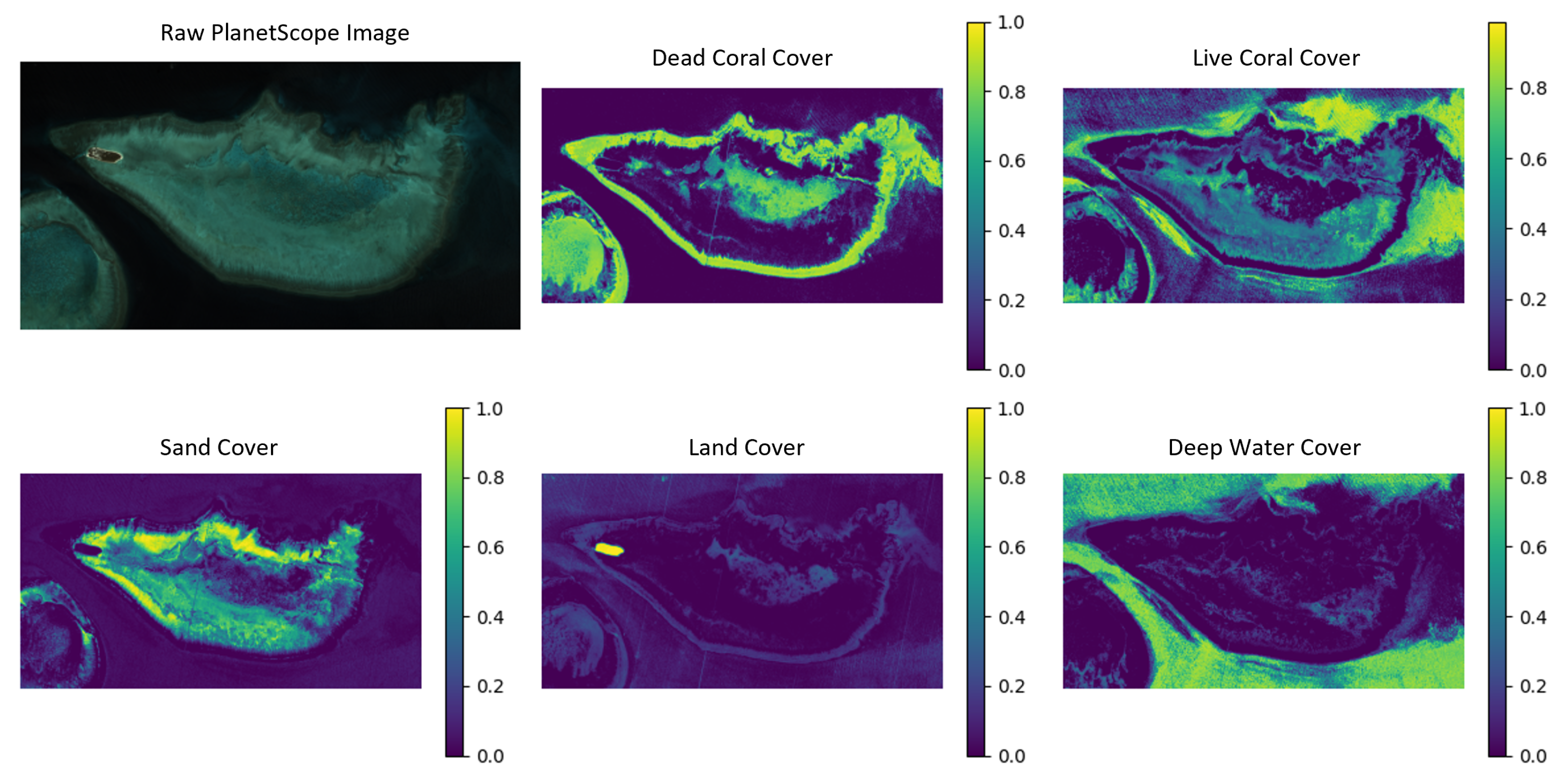
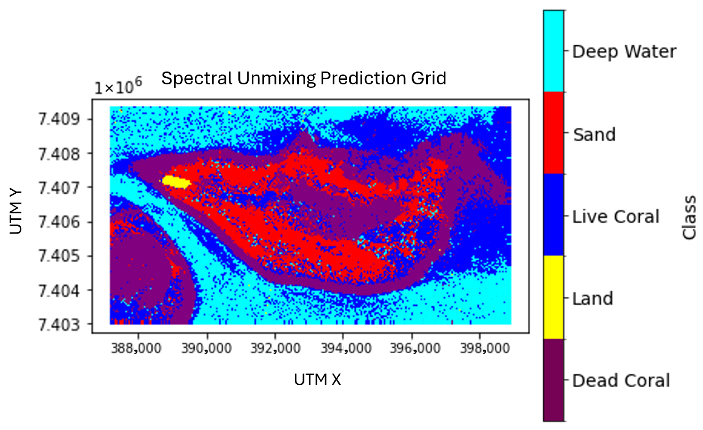
The results presented for the unmixing model were trained using only the first input configuration (the spectral data and derived spectral features), as explained in Section Preliminary Feature Analysis on Simple Method. Unlike the other models, the unmixing approach produces percent cover maps that estimate the sub-pixel proportion of each endmember class. These percent cover maps are shown in Figure 16, where dark purple indicates coverage and bright yellow indicates coverage of a given endmember. From these percent cover maps, a predicted benthic habitat map is derived by assigning each pixel the class corresponding to its highest abundance value (Figure 17). When compared to the ground truth dataset, this model achieved an overall accuracy of .
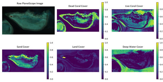
Figure 16.
Top left image: PlanetScope satellite image of Heron Island obtained on 24 October 2018. Remaining images: Sub-pixel percent cover maps for each class, where the color bar represents coverage (purple) to coverage (yellow).

Figure 17.
Results of the unmixing model, presented with the most dominant endmember for each pixel. Map is displayed in UTM coordinates, Zone 56S. The satellite image in Figure 2 serves as a reference.
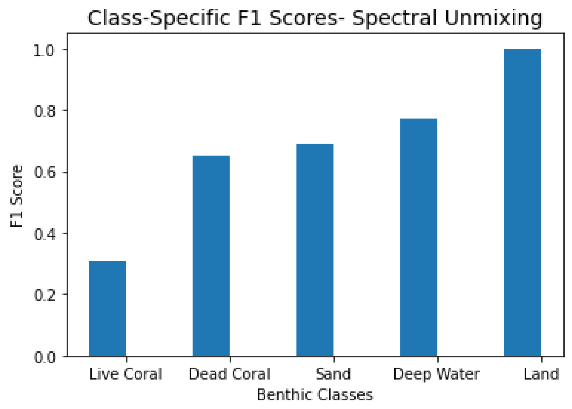
Class-specific F1 scores for this model are shown in Figure 18. Notably, this method achieved the highest F1 score for live coral among all approaches, suggesting that the unmixing framework more effectively captures the unique characteristics of this class. Performance for the other benthic classes is generally comparable to that of the other methods.
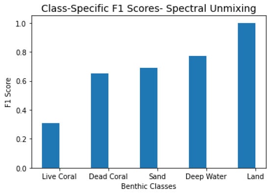
Figure 18.
Class-specific F1 scores for the unmixing model.
3.3. Benthic Cover Estimation
In addition to assessing pixel-level accuracy, it is also important to evaluate how each model represents the overall composition of benthic habitats across the study site. This provides insight into whether models are over- or under-predicting specific habitat types at the landscape scale, which is critical for ecological interpretation and habitat monitoring. To this end, we compared benthic cover estimates derived from each model, alongside confusion matrices that capture class-level agreement with ground truth, weighted by class-specific F1 scores.
Benthic class coverage estimates are presented for the best-performing model from each classification method. The top K-Means clustering model was the semi-supervised version trained exclusively on spectral data with computed band ratios and differences. The preferred AdaBoost model, selected for its ecological plausibility, was also trained only on the spectral data. Spectral unmixing was implemented as a single model trained on spectral data with derived features.
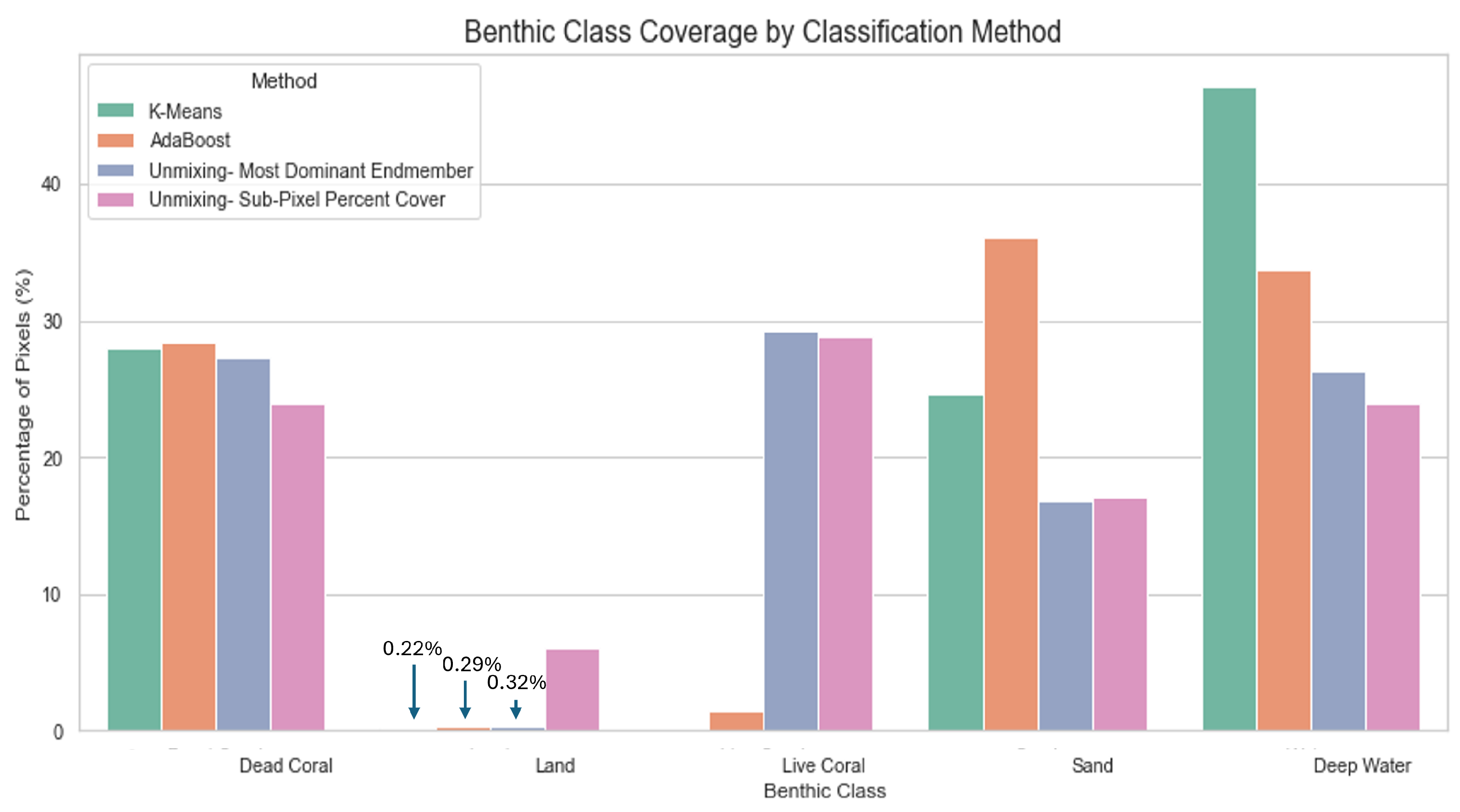
Figure 19 shows the proportion of total pixels assigned to each benthic class by each method for the entire study site. For spectral unmixing, we included both class coverage derived from the most dominant class per pixel and the total percent cover per class across the scene.
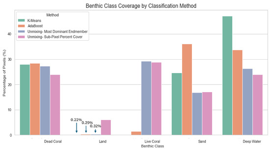
Figure 19.
Estimated benthic class coverage across the Heron Reef study site for each classification method. Coverage is expressed as the percentage of total pixels assigned to each class based on full-scene predictions.
Predicted benthic cover varied substantially across models and habitat types, revealing key differences in how each method interpreted the scene (Figure 19). Pixel-level estimates were highly variable across both methods and classes. Pixel-based classifiers like K-Means and AdaBoost often overrepresented spatially uniform classes like deep water and sand. For instance, AdaBoost predicted that sand and deep water dominated the site, with sand covering close to half the area, but estimated relatively little dead coral and almost no live coral. K-Means showed a similar pattern, though it predicted slightly more dead coral and failed to detect live coral entirely. In contrast, spectral unmixing estimated more balanced proportions, allowing it to retain ecologically important classes such as live coral that are easily overlooked in coarser classification schemes. It identified substantial areas of live coral (nearly a third of the site) while also moderating the extent of sand and deep water. Land was consistently predicted in small amounts across all models, though slightly elevated in the sub-pixel abundance outputs of the unmixing method.
These patterns suggest that spectral unmixing may better capture the fine-scale variation and mixed composition of coral reef habitats, whereas pixel-based classifiers may overrepresent spectrally dominant substrates and underrepresent complex or mixed habitats such as those observed in coral reefs.
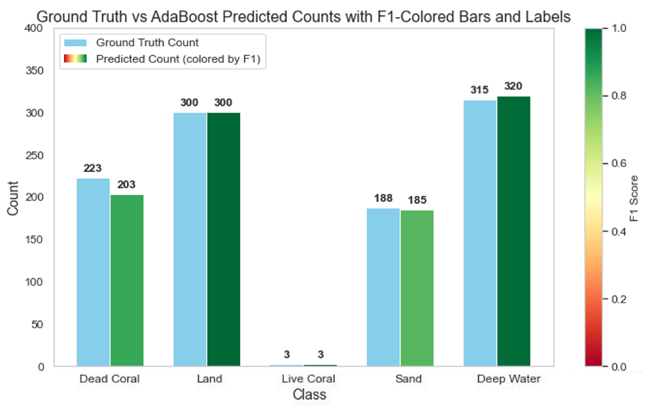
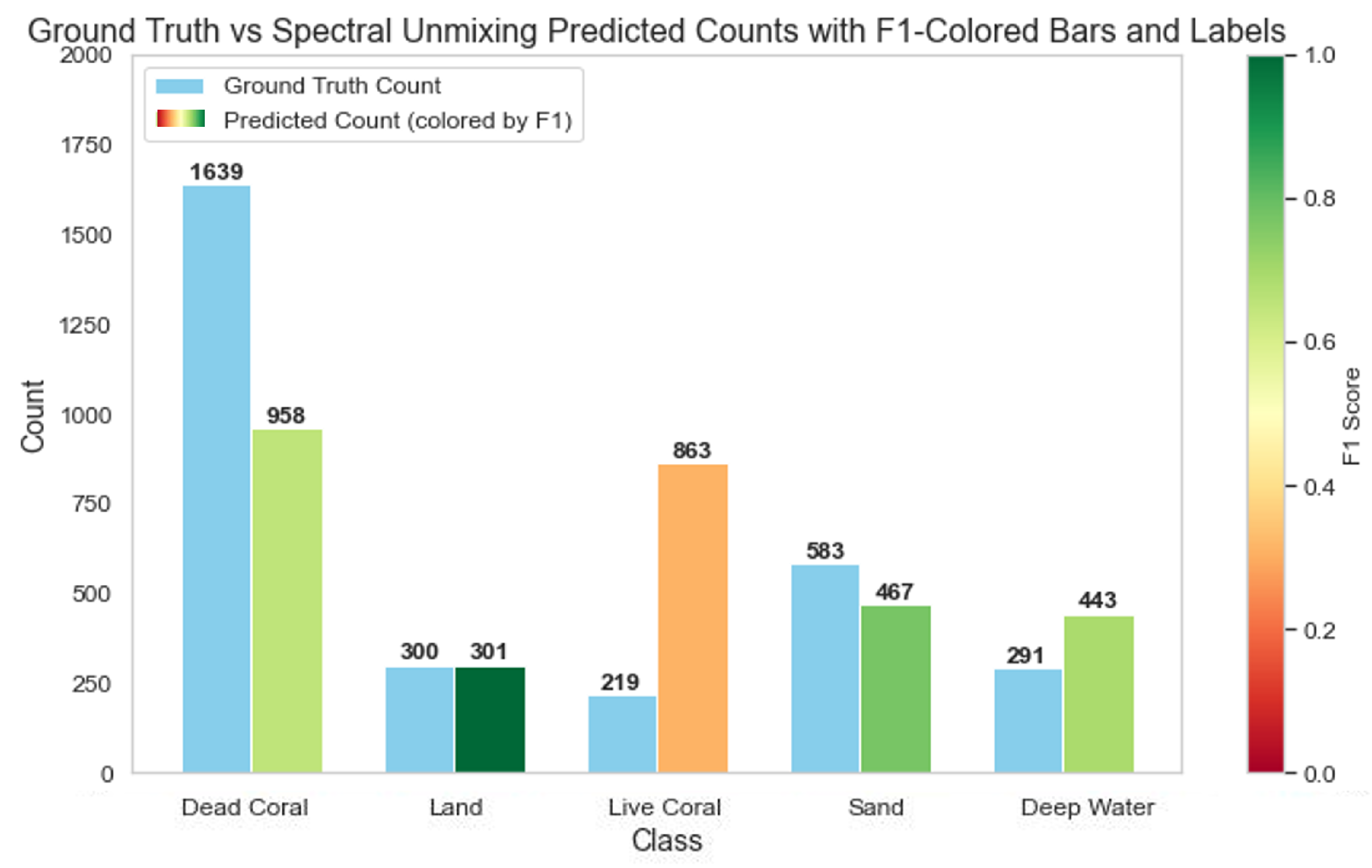
To further interpret these coverage estimates, we compared the number of predicted and ground truth pixels for each class across all methods. Figure 20, Figure 21 and Figure 22 visualize these comparisons by showing total predicted and actual pixel counts per class. We color-coded the predicted pixel counts by class-level F1 scores to evaluate class-specific performance, with green prediction bars indicating strong class-specific performance and high F1 scores. These plots helped assess model reliability by class and highlight patterns of over- or underprediction relative to the ground truth data.

Figure 20.
Comparison of K-Means clustering predictions and ground truth pixel counts per benthic class, color-coded by F1 score.

Figure 21.
Comparison of AdaBoost predictions and ground truth pixel counts per benthic class, color-coded by F1 score.
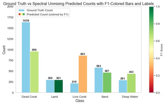
Figure 22.
Comparison of spectral unmixing predictions and ground truth pixel counts per benthic class, color-coded by F1 score.
K-Means clustering classified sand and dead coral with high F1 scores and small differences between predicted and actual pixel counts. Land was classified with near-perfect accuracy (F1 ). Deep water was also reasonably well predicted, with a moderate difference in pixel counts and a high F1 score. However, live coral was poorly classified, receiving an F1 of 0 despite a small difference in pixel counts. We believe this is a reflection of class sparsity rather than model failure.
The optimal AdaBoost model performed well overall, with particularly strong agreement for land and deep water, where predicted counts closely matched the ground truth and F1 scores were high. Live coral also showed good performance, achieving a high F1 score despite its small sample size. Sand exhibited good agreement, with only a slight underestimation, while dead coral was moderately underestimated relative to the ground truth.
Unlike the ML models, which required a training/testing split and therefore excluded a portion of the labeled pixels from evaluation, the unmixing method does not involve training. As a result, there are a larger number of examples per class. Performance for spectral unmixing varied considerably among classes. Land was predicted nearly perfectly, with a high F1 score and only 1 pixel difference between predicted and actual counts. In contrast, sand and deep water showed much larger discrepancies in pixel counts but still achieved high F1 scores. Dead coral and live coral proved more challenging. Dead coral was substantially underpredicted, while live coral was overpredicted. Both classes had correspondingly lower F1 scores, indicating reduced reliability for these ecologically important classes.
4. Discussion
This study explored the integration of remote sensing imagery with in situ observations to classify benthic habitats, comparing machine learning (ML) approaches and a novel nonlinear spectral unmixing algorithm developed via mathematical optimization. To our knowledge, this represents a new, purely mathematical method applied to benthic habitat mapping, offering sub-pixel percent cover estimates that better capture the ecological complexity of reef environments. We evaluated K-Means clustering, AdaBoost decision trees, and our spectral unmixing method, demonstrating the advantages of continuous fractional outputs over discrete classifications.
To enhance classification performance, we supplemented raw PlanetScope bands with derived features, including band ratios and differences, inspired by established remote sensing indices. These features improved results across all models. Incorporating ICESat-2 metrics yielded mixed results depending on the model, demonstrating the potential value and limitations of including seafloor-surface metrics. Recall that the AdaBoost model achieved a global accuracy of when trained on spectral and derived spectral data, and when trained using spectral, derived spectral, and ICESat-2 derived data. Although the expanded model showed a slight decrease in overall accuracy (), it produced broadly similar spatial patterns. These results suggest that while ICESat-2–derived metrics contribute additional structural information, they did not substantially improve classification performance in this case. In contrast, the spectral data AdaBoost model produced results more consistent with expected reef patterns. Recall that the K-Means model achieved a global accuracy of when trained on spectral and derived spectral data, and when trained using spectral, derived spectral, and ICESat-2 derived data. K-Means performance declined with the inclusion of ICESat-2 metrics ( reduction in accuracy), likely due to polygon-like artifacts introduced by the ICESat-2 surfaces, whereas spectral unmixing was minimally affected. The motivation for including ICESat-2 data was based on our analysis of the ground truth dataset, which revealed minimal spectral separability among key benthic classes, namely live coral, dead coral, and sand. Although the inclusion of ICESat-2 metrics did not improve classification performance in this study, these data were intended to provide additional structural information to help distinguish these spectrally similar classes. Overall, these results emphasize that the benefits of ancillary data are highly model-dependent and should be evaluated not only by numeric accuracy but also by their ecological validity.
Among the models tested, AdaBoost decision trees achieved the highest classification accuracy () when trained on spectral-only data. This model performed well across most classes, with high F1 scores across all classes. We attribute its success to its ability to learn complex patterns in the data that are inaccessible to more rigid mathematical models. K-Means clustering was moderately effective but less adaptable to mixed input data. The model’s low F1 score for live coral likely reflects the sparsity of this class in the ground truth data.
In contrast, the spectral unmixing model, while lower in overall accuracy, offers unique and powerful advantages for benthic mapping. Unlike the ML models, which produce discrete class labels, unmixing provides sub-pixel abundance estimates, offering a fundamentally richer and more ecologically realistic view of benthic composition. By quantifying the fractional coverage of each class within a pixel, the method captures fine-scale heterogeneity that conventional classifiers miss. In this region, the seafloor is patchy [53], and the unmixing method effectively captures both this patchiness and corals in deeper areas beyond the reef edge. This capability is particularly valuable for ecological assessments and long-term monitoring, where mixed-class pixels and unsampled regions are common. The resulting unmixing maps not only indicate the presence or absence of coral but also estimate percent cover, creating a baseline for more detailed habitat monitoring. Although sub-pixel validation was limited by the number of m photoquadrats, we anticipate that the model’s performance would improve substantially with more representative ground truth data, highlighting the strong potential of spectral unmixing for advancing coral reef mapping and management.
The limitations of the ground truth data played a significant role in model performance. Although statistical tests showed that most benthic classes are separable, several data quality issues complicated model training and interpretation. These included labeling conflicts among spectrally identical observations and insufficient representation of the macroalgae class, which made its removal from analysis necessary. Live coral was similarly underrepresented in the ground truth dataset and consistently underpredicted by ML models. In contrast, the spectral unmixing models estimated substantially higher live coral coverage (28.9–29.3%: Figure 19). While the results of the ML models suggest that low predictions of live coral may be a reflection of its actual sparsity, the unmixing model results suggest these low predictions may be due to underrepresentation in training data. These findings underscore a critical principle in ML-based applications: poor model performance often stems from data quality issues, such as underrepresented ground truth classes, not model inadequacy. In this study, strategic preprocessing, including careful label curation and feature engineering, proved critical to mitigating these issues. Data quality assessment is equally important as model architecture refinement, and acknowledging these constraints allows for appropriate interpretation of results.
Operationally, this study reflects the realities of working with imperfect and heterogeneous environmental data. We combined multispectral imagery, limited in situ observations, and interpolated ICESat-2 metrics to construct the most comprehensive dataset possible for Heron Reef, under the common assumption that all data sources were spatially coincident. However, in practice, the ICESat-2 and PlanetScope data differ in both spatial resolution and sampling geometry, and aligning these sources inherently introduces positional uncertainty. The ICESat-2 surfaces used here were interpolated from discrete along-track measurements into continuous representations using Voronoi polygons. This approach inevitably introduces spatial uncertainty but provides a practical means of associating ICESat-2 variables with PlanetScope imagery, reflecting the conditions under which most coral reef mapping efforts are conducted. Such errors are inherent to real-world remote sensing and cannot be fully eliminated. Rather than viewing these discrepancies as flaws, we recognize them as practical constraints of using operational data to model complex reef systems. Acknowledging and working within these limitations is essential for developing methods that remain realistic, transferable, and applicable across diverse, data-limited reef environments.
The depth in the study area ranges from approximately 0.5–10 m in regions where photoquadrats were collected. While most photoquadrats fall within relatively shallow reef areas where depth likely has minimal impact on observed benthic cover, deeper regions can still influence visibility and reflectance, particularly for substrates like live coral. This pattern is consistent with the physics of light attenuation in water: shallower features are more easily distinguished in the blue and green bands, while deeper features become increasingly difficult to detect. Additionally, NIR reflectance decreases rapidly with depth, becoming negligible below approximately 1 m and providing a reliable signal only in very shallow areas or over land [54]. Although the photoquadrats themselves do not inherently include depth measurements, we incorporated depth information from ICESat-2 into model training to help account for these potential effects. This demonstrates that, even with depth-related variation and limited spectral information, multispectral data can still provide ecologically meaningful insights when combined with robust unmixing approaches.
While spectral unmixing is typically applied to hyperspectral imagery, we chose to use multispectral data due to its broader availability. Multispectral sensors, such as those on PlanetScope satellites, offer practical advantages in terms of cost, spatial coverage, and temporal resolution. Although ground truth for live coral was limited, our spectral unmixing model performed better than the ML models and was able to capture live coral in unsampled, deeper locations, demonstrating the ecological value of this approach. This is a noteworthy outcome given that multispectral sensors have relatively few broad spectral bands, which can make it challenging to separate classes with similar spectral signatures (e.g., live coral, dead coral, macroalgae). That spectral overlap is a well-known limitation of multispectral data, yet our findings demonstrate that spectral unmixing applied to multispectral data yields valuable ecological insights when supported by careful preprocessing and robust training data. Nonetheless, the use of hyperspectral imagery, which contains hundreds of contiguous bands, could significantly improve the ability of unmixing algorithms to discriminate among benthic classes with subtle spectral differences. This improvement depends on whether at least one narrow band captures a distinct reflectance feature that clearly differentiates one class from another. As hyperspectral missions become more widely available, future applications of this method may benefit from leveraging the increased spectral resolution to improve classification accuracy, especially in complex reef environments.
The results of this study are promising, demonstrating strong model performance under favorable environmental conditions. Heron Island’s shallow depth, high water clarity, and well-defined reef edges created near-ideal conditions for optical remote sensing, enhancing spectral separability and minimizing confounding effects such as water column interference. These favorable conditions likely contributed to the success of the models, but they also highlight the importance of testing performance across a broader range of reef environments. In particular, validation in regions with more representative training datasets, especially those with high densities of live coral, could provide additional insight into the reliability of spectral unmixing and machine learning approaches. Applying these methods in settings with greater depth, higher turbidity, or more complex geomorphology will provide important opportunities to test the robustness, adaptability, and scalability of the approaches developed here. Improving the representation of underrepresented classes, such as live coral and macroalgae, within ground truth datasets should also be prioritized. Taken together, these steps will further strengthen model performance and enhance the ecological relevance and conservation utility of remote sensing–based habitat classification across diverse reef systems worldwide.
5. Conclusions
This study evaluated three classification approaches—K-Means clustering, AdaBoost decision trees, and a novel spectral unmixing method—for mapping benthic habitats using remote sensing imagery, engineered spectral features, and ICESat-2-derived parameters. The nonlinear spectral unmixing approach represents a significant methodological advancement: it operates directly on multispectral imagery without requiring water column corrections and eliminates the need for site-specific environmental parameters that have traditionally limited the scalability of reef mapping methods. While AdaBoost achieved the highest discrete classification accuracy, the novel unmixing method uniquely provides sub-pixel percent cover estimates, capturing the mixed benthic composition within a pixel. This capability offers fundamentally richer ecological insights into benthic composition and habitat structure than traditional hard classification methods, making it particularly valuable for characterizing complex reef environments. The novelty of the unmixing approach lies in its ability to integrate spectral and other derived information to produce ecologically meaningful outputs that are potentially more cost-effective for large-scale monitoring. Model performance was limited by ground truth data quality, particularly the underrepresentation of key classes. These findings underscore the importance of high-quality ground truth data and intentional preprocessing. Overall, our findings demonstrate the potential of combining multispectral imagery with ICESat-2-derived metrics and nonlinear spectral unmixing to advance reef mapping. Generalizing to other reef systems will require careful consideration of environmental variability and deeper, more turbid conditions. Future work should focus on expanding model testing to more complex environments, improving data coverage for rare or spectrally similar classes, and further developing the mathematical framework of nonlinear spectral unmixing for broader marine applications.
Author Contributions
Conceptualization, G.A.T., M.L., K.L. and J.A.D.; Methodology, G.A.T., M.L. and K.L.; Software, G.A.T.; Validation, G.A.T. and J.A.D.; Formal Analysis, G.A.T., M.L. and K.L.; Investigation, G.A.T.; Data Curation, G.A.T.; Writing—Original Draft Preparation, G.A.T.; Writing—Review & Editing, G.A.T., M.L., K.L., and J.A.D.; Visualization, G.A.T.; Supervision, M.L., K.L. and J.A.D.; Project Administration, G.A.T.; Funding Acquisition, J.A.D. All authors have read and agreed to the published version of the manuscript.
Funding
This research was funded by the National Oceanic and Atmospheric Administration under Grant number NA20NOS4000196.
Data Availability Statement
We thank Planet Labs for providing the PlanetScope satellite imagery used in this study, available via the Planet Application Program Interface: In Space for Life on Earth. San Francisco, CA (https://api.planet.com. The Roelfsema photoquadrats can be found at https://doi.org/10.1594/PANGAEA.894801, accessed on 27 September 2024 (Creative Commons Attribution 4.0 International, accessed on 27 September 2024) and were not modified. ICESat-2 data is available for download from https://nsidc.org/data/icesat-2/data, accessed on 30 October 2024.
Acknowledgments
During the preparation of this work, the authors used Claude and Grammarly to improve language, readability, and grammar. After using this tool/service, the authors reviewed and edited the content as needed and take full responsibility for the content of the publication.
Conflicts of Interest
The authors declare no conflicts of interest.
Appendix A. Interpolated Surfaces of ICESat-2 Derived Variable
To integrate ICESat-2-derived features with PlanetScope imagery across the full study area, continuous surfaces were generated from the discrete along-track ICESat-2 measurements using a Voronoi polygon (also called Thiessen polygon) approach, following the methodology described in our previous work [23]. Each ICESat-2 track was first processed to extract bathymetric points and calculate per-window metrics including rugosity, slope, and depth. Voronoi polygons were then constructed around the center of each 20 m along-track window, defining areas of influence such that all locations within a polygon were assigned the values of the nearest ICESat-2 window. Figure 9 in [23] illustrates this construction.
The resulting surfaces for rugosity and slope can be found in Figure A1. Rugosity and slope values were grouped into low, medium, and high categories for visualization. Category thresholds were defined using the 33rd and 66th percentiles of the variable distributions: values at or below the 33rd percentile were classified as low, values between the 33rd and 66th percentiles as medium, and values above the 66th percentile as high. While this process does not produce a smooth surface, it preserves the along-track sampling structure of ICESat-2, accounts for the sparse and irregular coverage of tracks, and effectively captures large-scale variability in seafloor structure relevant for coral reef mapping.

Figure A1.
Interpolated surfaces of rugosity and slope derived from ICESat-2 data.
Figure A1.
Interpolated surfaces of rugosity and slope derived from ICESat-2 data.

References
- Day, J. Protecting Australia’s Great Barrier Reef. Solutions 2011, 2, 56–66. [Google Scholar]
- O’Mahony, J.; Simes, R.; Redhill, D.; Heaton, K.; Atkinson, C.; Hayward, E.; Nguyen, M. At What Price? The Economic, Social and Icon Value of the Great Barrier Reef. Technical Report, Deloitte Access Economics, Australia. 2017. Available online: https://hdl.handle.net/11017/3205 (accessed on 20 October 2025).
- De’ath, G.; Fabricius, K.E.; Sweatman, H.; Puotinen, M. The 27–year decline of coral cover on the Great Barrier Reef and its causes. Proc. Natl. Acad. Sci. USA 2012, 109, 17995–17999. [Google Scholar] [CrossRef]
- Van An, N.; Quang, N.H.; Son, T.P.; An, T.T. High-resolution benthic habitat mapping from machine learning on PlanetScope imagery and ICESat-2 data. Geocarto Int. 2023, 38, 2184875. [Google Scholar] [CrossRef]
- Gapper, J.J.; Maharjan, S.; Li, W.; Linstead, E.; Tiwari, S.P.; Qurban, M.A.; El-Askary, H. A generalized machine learning model for long-term coral reef monitoring in the Red Sea. Heliyon 2024, 10, e38249. [Google Scholar] [CrossRef]
- He, M.; He, J.; Zhou, Y.; Sun, L.; He, S.; Liu, C.; Gu, Y.; Li, P. Coral reef applications of Landsat-8: Geomorphic zonation and benthic habitat mapping of Xisha Islands, China. Giscience Remote Sens. 2023, 60, 2261213. [Google Scholar] [CrossRef]
- Hedley, J.D.; Roelfsema, C.; Brando, V.; Giardino, C.; Kutser, T.; Phinn, S.; Mumby, P.J.; Barrilero, O.; Laporte, J.; Koetz, B. Coral reef applications of Sentinel-2: Coverage, characteristics, bathymetry and benthic mapping with comparison to Landsat 8. Remote Sens. Environ. 2018, 216, 598–614. [Google Scholar] [CrossRef]
- Xu, J.; Zhao, J.; Wang, F.; Chen, Y.; Lee, Z. Detection of Coral Reef Bleaching Based on Sentinel-2 Multi-Temporal Imagery: Simulation and Case Study. Front. Mar. Sci. 2021, 8, 584263. [Google Scholar] [CrossRef]
- Dung, T.; Anh, L.; Nga, D. Coral Reefs Detecting with Artificial Neural Network Classification and PlanetScope Imagery in Cu Lao Xanh Island, Binh Dinh province. IOP Conf. Ser. Earth Environ. Sci. 2023, 1170, 012024. [Google Scholar] [CrossRef]
- Burns, C.; Bollard, B.; Narayanan, A. Machine-Learning for Mapping and Monitoring Shallow Coral Reef Habitats. Remote Sens. 2022, 14, 2666. [Google Scholar] [CrossRef]
- Lu, Z.; Zhu, W.; Lei, D.; Zhu, Y.; Chen, Y.; Yue, Z.; Wu, Z. Water Depth Correction-Based Classification Combination Method for Extracting Shallow Sea Reef Geomorphological Information: A Case Study of Xisha Chau and Zhaoshu Island. J. Mar. Sci. Eng. 2025, 13, 300. [Google Scholar] [CrossRef]
- White, E.; Mohseni, F.; Amani, M. Coral Reef mapping using remote sensing techniques and a supervised classification algorithm. Adv. Environ. Eng. Res. 2021, 2, 28. [Google Scholar] [CrossRef]
- Panjaitan, J.P.; Mahendratama, G.; Siregar, V. Benthic habitats mapping in Pari Island, Kepulauan Seribu, Indonesia using drone and sentinel-2B imagery with object based image analysis method. BIO Web Conf. 2025, 168, 05004. [Google Scholar] [CrossRef]
- Radford, B.; Puotinen, M.; Sahin, D.; Boutros, N.; Wyatt, M.; Gilmour, J. A remote sensing model for coral recruitment habitat. Remote Sens. Environ. 2024, 311, 114231. [Google Scholar] [CrossRef]
- da Silveira, C.B.L.; Strenzel, G.M.R.; Maida, M.; Gaspar, A.L.B.; Ferreira, B.P. Coral Reef Mapping with Remote Sensing and Machine Learning: A Nurture and Nature Analysis in Marine Protected Areas. Remote Sens. 2021, 13, 2907. [Google Scholar] [CrossRef]
- Nimalan, K.; Thanikachalam, M.; Usha, T. Estimating the fractional abundance of coral reef benthic compositions using linear spectral unmixing. Int. J. Fish. Aquat. Stud. 2020, 8, 181–186. [Google Scholar] [CrossRef]
- Hedley, J.D.; Mumby, P.J. A remote sensing method for resolving depth and subpixel composition of aquatic benthos. Limnol. Oceanogr. 2003, 48, 480–488. [Google Scholar] [CrossRef]
- Lee, Z.; Carder, K.L.; Mobley, C.D.; Steward, R.G.; Patch, J.S. Hyperspectral remote sensing for shallow waters. I. A semianalytical model. Appl. Opt. 1998, 37, 6329–6338. [Google Scholar] [CrossRef]
- Lee, Z.; Carder, K.L.; Mobley, C.D.; Steward, R.G.; Patch, J.S. Hyperspectral remote sensing for shallow waters: 2. Deriving bottom depths and water properties by optimization. Appl. Opt. 1999, 38, 3831–3843. [Google Scholar] [CrossRef]
- Torres-Madronero, M.; Velez-Reyes, M.; Goodman, J. Subsurface unmixing for benthic habitat mapping using hyperspectral imagery and lidar-derived bathymetry. Proc. SPIE- Int. Soc. Opt. Eng. 2014, 9088, 90880M. [Google Scholar] [CrossRef]
- Goodman, J.; Ustin, S. Classification of benthic composition in a coral reef environment using spectral unmixing. J. Appl. Remote Sens. 2007, 1, 011501. [Google Scholar] [CrossRef]
- Cai, J.; Chatoux, H.; Boust, C.; Mansouri, A. Extending the Unmixing methods to Multispectral Images. Color Imaging Conf. 2021, 2021, 311–316. [Google Scholar] [CrossRef]
- Trudeau, G.A.; Lowell, K.; Dijkstra, J.A. Coral reef detection using ICESat-2 and machine learning. Ecol. Inform. 2025, 87, 103099. [Google Scholar] [CrossRef]
- Planet Team. Planet Application Program Interface: In Space for Life on Earth. San Francisco, CA, USA, 2025. Available online: https://api.planet.com (accessed on 5 November 2024).
- Planet Team. PlanetScope Imagery Product Specification. Technical report, Planet Labs PBC. 2023. Available online: https://docs.planet.com/data/imagery/planetscope/techspec/ (accessed on 16 October 2024).
- Roelfsema, C.M.; Kovacs, E.M.; Markey, K.; Phinn, S.R. Benthic and Substrate Cover Data Derived from Field Photo-Transect Surveys for the Heron Reef Flat and Slope Areas (2018-11); PANGAEA, 2019. Available online: https://doi.org/10.1594/PANGAEA.903767 (accessed on 27 September 2024).
- Roelfsema, C.M.; Phinn, S.R. Integrating field data with high spatial resolution multispectral satellite imagery for calibration and validation of coral reef benthic community maps. J. Appl. Remote Sens. 2010, 4, 043527. [Google Scholar] [CrossRef]
- National Snow and Ice Data Center. ICESat-2. 2024. Available online: https://nsidc.org/data/icesat-2 (accessed on 20 February 2025).
- Neumann, T.A.; Brenner, A.; Hancock, D.; Robbins, J.; Gibbons, A.; Lee, J.; Harbeck, K.; Saba, J.; Luthcke, S.; Rebold, T. Ice, Cloud, and Land Elevation Satellite (ICESat-2) Project Algorithm Theoretical Basis Document (ATBD) for Global Geolocated Photons (ATL03); Technical Report; NASA Goddard Space Flight Center: Greenbelt, MD, USA, 2022. [Google Scholar] [CrossRef]
- Phinn, S.R.; Roelfsema, C.M.; Mumby, P.J. Multi-scale, object-based image analysis for mapping geomorphic and ecological zones on coral reefs. Int. J. Remote Sens. 2012, 33, 3768–3797. [Google Scholar] [CrossRef]
- United States Federal Geographic Data Committee. Coastal and Marine Ecological Classification Standard. 2012. Available online: https://repository.library.noaa.gov/view/noaa/27552 (accessed on 1 November 2024).
- Holden, H.; LeDrew, E. Spectral Discrimination of Healthy and Non-Healthy Corals Based on Cluster Analysis, Principal Components Analysis, and Derivative Spectroscopy. Remote Sens. Environ. 1998, 65, 217–224. [Google Scholar] [CrossRef]
- Hochberg, E.J.; Atkinson, M.J.; Andréfouët, S. Spectral reflectance of coral reef bottom-types worldwide and implications for coral reef remote sensing. Remote Sens. Environ. 2003, 85, 159–173. [Google Scholar] [CrossRef]
- Nurdin, N.; Komatsu, T.; Yamano, H.; Arafat, G.; Rani, C.; AS, M.A. Spectral response of the coral rubble, living corals, and dead corals: Study case on the Spermonde Archipelago, Indonesia. In Proceedings of the Remote Sensing of the Marine Environment II, Kyoto, Japan, 29 October–1 November 2012; Frouin, R.J., Ebuchi, N., Pan, D., Saino, T., Eds.; International Society for Optics and Photonics, SPIE: Bellingham, WA, USA, 2012; Volume 8525, p. 85251A. [Google Scholar] [CrossRef]
- QGIS Development Team. QGIS Geographic Information System. Open Source Geospatial Foundation Project, [Software]. 2024. Available online: https://www.qgis.org/ (accessed on 19 October 2024).
- JMP Statistical Discovery LLC. JMP® Pro 18; JMP Statistical Discovery LLC: Cary, NC, USA, 2025. [Google Scholar]
- Landsat Missions. Landsat Normalized Difference Vegetation Index. Available online: https://www.usgs.gov/landsat-missions/landsat-normalized-difference-vegetation-index (accessed on 9 June 2025).
- Landsat Missions. Landsat Normalized Difference Moisture Index. Available online: https://www.usgs.gov/landsat-missions/normalized-difference-moisture-index (accessed on 9 June 2025).
- Prajisha, C.; Achu, A.; Joseph, S. Chapter 9—Landslide susceptibility modeling using a generalized linear model in a tropical river basin of the Southern Western Ghats, India. In Water, Land, and Forest Susceptibility and Sustainability; Chatterjee, U., Pradhan, B., Kumar, S., Saha, S., Zakwan, M., Fath, B.D., Fiscus, D., Eds.; Elsevier: Amsterdam, The Netherlands, 2023; Volume 1, Science of Sustainable Systems; pp. 237–266. [Google Scholar] [CrossRef]
- Lyons, M.; Larsen, K.; Skone, M. CoralMapping/AllenCoralAtlas: v1.3. 2022. Available online: https://doi.org/10.5281/zenodo.6622015 (accessed on 13 April 2025).
- Sinaga, K.P.; Yang, M.S. Unsupervised K-Means Clustering Algorithm. IEEE Access 2020, 8, 80716–80727. [Google Scholar] [CrossRef]
- Schapire, R.E. Explaining AdaBoost. In Empirical Inference: Festschrift in Honor of Vladimir N. Vapnik; Schölkopf, B., Luo, Z., Vovk, V., Eds.; Springer: Berlin/Heidelberg, Germany, 2013; pp. 37–52. [Google Scholar] [CrossRef]
- Pedregosa, F.; Varoquaux, G.; Gramfort, A.; Michel, V.; Thirion, B.; Grisel, O.; Blondel, M.; Prettenhofer, P.; Weiss, R.; Dubourg, V.; et al. Scikit-learn: Machine Learning in Python. J. Mach. Learn. Res. 2011, 12, 2825–2830. [Google Scholar]
- Nembrini, S.; König, I.R.; Wright, M.N. The revival of the Gini importance? Bioinformatics 2018, 34, 3711–3718. [Google Scholar] [CrossRef]
- Pour, A.B.; Ranjbar, H.; Sekandari, M.; Abd El-Wahed, M.; Hossain, M.S.; Hashim, M.; Yousefi, M.; Zoheir, B.; Wambo, J.D.T.; Muslim, A.M. Remote sensing for mineral exploration. In Geospatial Analysis Applied to Mineral Exploration; Pour, A.B., Parsa, M., Eldosouky, A.M., Eds.; Elsevier: Amsterdam, The Netherlands, 2023; pp. 17–149. [Google Scholar] [CrossRef]
- Sánchez, A.; Marro, M.; Marsal, M.; Zacchetti, S.; de Oliveira, R.; Loza-Alvarez, P.; De Juan, A. Linear unmixing protocol for hyperspectral image fusion analysis applied to a case study of vegetal tissues. Sci. Rep. 2021, 11, 18665. [Google Scholar] [CrossRef]
- Eugenio, F.; Marcello, J.; Martin, J.; Rodríguez-Esparragón, D. Benthic Habitat Mapping Using Multispectral High-Resolution Imagery: Evaluation of Shallow Water Atmospheric Correction Techniques. Sensors 2017, 17, 2639. [Google Scholar] [CrossRef]
- Ghrefat, H.; Awawdeh, M.; Howari, F.; Al-Rawabdeh, A. Chapter 12—Mineral exploration using multispectral and hyperspectral remote sensing data. In Geoinformatics for Geosciences; Stathopoulos, N., Tsatsaris, A., Kalogeropoulos, K., Eds.; Earth Observation; Elsevier: Amsterdam, The Netherlands, 2023; pp. 197–222. [Google Scholar] [CrossRef]
- Grammerly. F1 Score in Machine Learning: How to Calculate, Apply, and Use It Effectively. 2025. Available online: https://www.grammarly.com/blog/ai/what-is-f1-score/ (accessed on 13 April 2025).
- Xu, Y.; Vaughn, N.R.; Knapp, D.E.; Martin, R.E.; Balzotti, C.; Li, J.; Foo, S.A.; Asner, G.P. Coral Bleaching Detection in the Hawaiian Islands Using Spatio-Temporal Standardized Bottom Reflectance and Planet Dove Satellites. Remote Sens. 2020, 12, 3219. [Google Scholar] [CrossRef]
- Brown, K.; Bender-Champ, D.; Hoegh-Guldberg, O.; Dove, S. Seasonal shifts in the competitive ability of macroalgae influence the outcomes of coral–algal competition. R. Soc. Open Sci. 2020, 7, 201797. [Google Scholar] [CrossRef] [PubMed]
- Roelfsema, C.; Kovacs, E.; Markey, K.; Vercelloni, J.; Rodriguez-Ramirez, A.; Lopez-Marcano, S.; Gonzalez-Rivero, M.; Hoegh-Guldberg, O.; Phinn, S. Benthic and coral reef community field data for Heron Reef, Southern Great Barrier Reef, Australia, 2002–2018. Sci. Data 2021, 8, 84. [Google Scholar] [CrossRef]
- Foo, S.A.; Asner, G.P. Scaling Up Coral Reef Restoration Using Remote Sensing Technology. Front. Mar. Sci. 2019, 6, 79. [Google Scholar] [CrossRef]
- Kou, L.; Labrie, D.; Chylek, P. Refractive indices of water and ice in the 0.65–2.5 µm spectral range. Appl. Opt. 1993, 32, 3531–3540. [Google Scholar] [CrossRef]
Disclaimer/Publisher’s Note: The statements, opinions and data contained in all publications are solely those of the individual author(s) and contributor(s) and not of MDPI and/or the editor(s). MDPI and/or the editor(s) disclaim responsibility for any injury to people or property resulting from any ideas, methods, instructions or products referred to in the content. |
© 2025 by the authors. Licensee MDPI, Basel, Switzerland. This article is an open access article distributed under the terms and conditions of the Creative Commons Attribution (CC BY) license (https://creativecommons.org/licenses/by/4.0/).


