Highlights
- What are the main findings?
- The proposed CResDAE model, which integrates a channel attention mechanism and deep residual modules, demonstrates superior performance in hyperspectral unmixing compared to both conventional and deep learning-based methods.
- Application of CResDAE to real GF-5 satellite data from Yunnan successfully identifies key surface materials, including Forest, Grassland, Silicate, Carbonate, and Sulfate.
- What is the implication of the main finding?
- The model provides a more interpretable and effective tool for geological surveys by explicitly addressing the limitations of band selection and physical constraints in existing unmixing methods.
- It offers reliable data support for mineral exploration in covered regions, enhancing the ability to analyze surface material composition quantitatively.
Abstract
Hyperspectral unmixing aims to extract pure spectral signatures (endmembers) and estimate their corresponding abundance fractions from mixed pixels, enabling quantitative analysis of surface material composition. However, in geological mineral exploration, existing unmixing methods often fail to explicitly identify informative spectral bands, lack inter-layer information transfer mechanisms, and overlook the physical constraints intrinsic to the unmixing process. These issues result in limited directionality, sparsity, and interpretability. To address these limitations, this paper proposes a novel model, CResDAE, based on a deep autoencoder architecture. The encoder integrates a channel attention mechanism and deep residual modules to enhance its ability to assign adaptive weights to spectral bands in geological hyperspectral unmixing tasks. The model is evaluated by comparing its performance with traditional and deep learning-based unmixing methods on synthetic datasets, and through a comparative analysis with a nonlinear autoencoder on the Urban hyperspectral scene. Experimental results show that CResDAE consistently outperforms both conventional and deep learning counterparts. Finally, CResDAE is applied to GF-5 hyperspectral imagery from Yunnan Province, China, where it effectively distinguishes surface materials such as Forest, Grassland, Silicate, Carbonate, and Sulfate, offering reliable data support for geological surveys and mineral exploration in covered regions.
1. Introduction
Hyperspectral remote sensing (HRS) is a multidimensional information acquisition technology that integrates imaging and spectroscopy. It enables the simultaneous acquisition of two-dimensional spatial information and a third spectral dimension, resulting in a hyperspectral data cube composed of continuous, narrow spectral bands with high spectral resolution [1,2,3]. HRS has been widely applied in various fields such as image processing [4], environmental monitoring [5], agricultural management [6], urban planning [7], geological mapping [8], and mineral prospecting [9].
However, due to the limited spatial resolution of sensors and the influence of complex surface environments—such as areas covered by vegetation [10,11]—most pixels in real-world hyperspectral images are mixtures of multiple ground materials, known as mixed pixels [12,13]. This spectral mixing phenomenon significantly reduces the analytical accuracy of hyperspectral data and limits its application in high-precision recognition tasks. To address this issue, hyperspectral unmixing techniques have been developed. The core objective of hyperspectral unmixing is to decompose mixed pixels into pure spectral signatures (endmembers) and their corresponding abundance fractions, thereby enabling quantitative analysis of surface material composition [14]. Depending on the underlying mixing models, hyperspectral unmixing can be categorized into linear spectral mixture models [15,16] and nonlinear spectral mixture models [17,18]. From the methodological perspective, unmixing approaches can be broadly classified into geometry-based methods [19,20], statistical modeling methods [21,22], and optimization-based methods [23,24]. In recent years, with the rapid development of big data and artificial intelligence technologies, deep learning methods such as Convolutional Neural Networks (CNN) [25,26,27], Graph Neural Networks (GNN) [28,29], Transformer [30,31], and Autoencoders (AE) [32,33] have been increasingly applied to hyperspectral unmixing tasks. Among them, the autoencoder is a fundamental deep learning architecture commonly used in hyperspectral unmixing, typically consisting of two main components: an encoder and a decoder. The encoder is responsible for extracting low-dimensional latent features to estimate abundance maps, while the decoder reconstructs the original input and retrieves the endmember matrix from these latent features. Numerous AE- or CNN-based variants have been proposed in the recent literature. Yu [34] introduced a multistage convolutional autoencoder network (MSNet) for hyperspectral analysis and demonstrated its robustness in addressing ill-posed decomposition problems. Wang [35] proposed an adaptive spectral–spatial attention autoencoder network (SSANet), which leverages the geometric characteristics of endmembers in hyperspectral images and incorporates abundance sparsity constraints, achieving competitive results in terms of root mean square error and spectral angle distance. Qu and Qi [36] developed a so-called sparse unlinked denoising autoencoder, in which the encoder and decoder are designed independently. The denoising ability is embedded into the network optimization process via a denoising constraint, and the encoder is regularized using an l21-norm to reduce redundant endmembers and minimize reconstruction error. Li and Zheng [37] proposed a model-informed multistage unsupervised network, by lever aging both deep image prior (DIP) and degradation model information, achieving significant progress in hyperspectral image super-resolution.
In the field of geological mineral exploration, hyperspectral unmixing has also demonstrated significant application value [38,39,40]. Different rock and mineral types exhibit distinct spectral absorption features, and hyperspectral imaging enables non-contact, large-scale identification of mineral types and distributions. However, due to intense surface rock weathering, mixed spectral characteristics often emerge, making it difficult for traditional classification methods to achieve accurate identification [41]. Hyperspectral unmixing offers an effective means to analyze mixed spectra in complex geological settings, isolating target minerals from background materials and thereby improving the accuracy of mineral exploration [42,43]. Attallah [44] proposed an optimized 3D–2D CNN model for automatic mineral identification and classification, which achieved outstanding performance and established a new benchmark for robust feature extraction and classification. Zhang [45] applied collaborative sparse unmixing to estimate mineral abundances in the Eberswalde crater delta on Mars, achieving promising unmixing results. Moreover, by integrating geological background information [46,47] and geochemical modeling approaches [48,49], unmixing results can be further used to construct mineralization alteration maps, assist in the delineation of anomalous mineralized zones, predict target ore bodies, and support metallogenic model analysis—thus significantly enhancing the efficiency and intelligence of geological exploration.
However, in the context of geological mineral exploration, existing hyperspectral unmixing studies exhibit several key limitations: (1) They typically fail to explicitly identify which spectral bands are more informative, effectively assuming that all bands contribute equally to endmember representation—an unrealistic simplification in geological scenarios; (2) They lack cross-layer information propagation, resulting in instability and increased training difficulty when dealing with highly nonlinear or locally sparse mineral distributions; (3) They often ignore physical constraints inherent in the unmixing process, resulting in non-sparse abundance maps, spectral bias, and distorted outputs due to insufficient modeling of directionality, sparsity, and interpretability.
To address these challenges, we propose the CResDAE model, which is based on a deep autoencoder architecture. By incorporating a channel attention mechanism and deep residual encoder modules into the encoder section, the model enhances weight allocation across spectral bands for hyperspectral unmixing tasks in geological applications. To validate the model’s effectiveness, we compared and evaluated its unmixing performance against traditional unmixing methods and deep learning models on a synthetic hyperspectral dataset. Subsequently, we contrasted the unmixing results of the Nonlinear Autoencoder (NAE) and CResDAE on urban hyperspectral imagery. Results demonstrate that the CResDAE model outperforms other models across all evaluation metrics. Finally, the model was applied to real Gaofen-5 hyperspectral imagery of Yunnan Province, China, achieving satisfactory unmixing and abundance inversion results. This provides decision-making support and technical backing for future geological prospecting in the study area.
2. Materials and Methods
In this study, the Urban hyperspectral image data and the corresponding endmember spectra of ground objects were first acquired. These spectral data were then used to construct a simulated hyperspectral dataset. Subsequently, a variety of unmixing models—including traditional methods such as MVC-NMF, VCA+K-Hype, LinearAE, ConvAE, and NAE, as well as the proposed CResDAE—were applied to the simulated dataset for unmixing performance evaluation and comparison. Afterward, a comparative experiment between NAE and CResDAE was conducted on the real Urban hyperspectral image. Finally, the proposed CResDAE model was applied to GF-5 hyperspectral imagery acquired from Yunnan Province, China. The overall technical workflow is illustrated in Figure 1.

Figure 1.
Technical workflow of the proposed hyperspectral unmixing approach.
The CResDAE model primarily incorporates several key methods, including linear and nonlinear spectral mixture models, deep autoencoder network, channel attention module, and deep residual encoder architecture.
2.1. Nonlinear Spectral Model
For the Linear Mixture Model (LMM), the hyperspectral unmixing process can be mathematically expressed as:
where is the observed hyperspectral image matrix with L spectral bands and n pixels, and denotes the additive noise matrix. is the endmember matrix, where each column represents the spectral signature of a distinct endmember. is the corresponding abundance matrix, subject to two physical constraints: the Abundance Nonnegativity Constraint (ANC) and the Abundance Sum-to-One Constraint (ASC), as follows:
where aij denotes the proportion of the j-th endmember in the i-th pixel, and p represents the total number of endmembers. These constraints ensure that the abundance values represent valid proportions of endmembers in each pixel.
The Linear Mixture Model (LMM) is well-suited for simple scenarios in which the incident light interacts with surface materials only once. However, when the incident light interacts with multiple materials, it becomes necessary to consider the Nonlinear Mixture Model (NLMM) [50]. NLMM provides a more realistic representation of the complex interactions between light and materials. It assumes that before being captured by the sensor, the incident light may undergo multiple reflections, scatterings, or transmissions among different substances, resulting in spectral features that are nonlinearly combined.
Building upon the Linear Spectral Mixture Model, this study also incorporates the Bilinear Mixture Model and the Post-Nonlinear Mixture Model [51]. The bilinear model is a type of nonlinear spectral mixture model that accounts for interactions between materials. In addition to the linear combination of endmember spectra, it introduces pairwise multiplicative terms between endmembers to simulate the interaction of light between two different materials. A commonly used mathematical formulation of the bilinear model is expressed as follows:
where x denotes the observed spectrum, ei represents the spectral signature of the i-th endmember, and ai is its corresponding abundance. The parameter controls the strength of the nonlinear interactions. The symbol denotes the Hadamard product, i.e., element-wise multiplication, and n represents the noise term. The first term corresponds to the standard linear component as in LMM, while the second term serves as a nonlinear compensation term, capturing optical coupling effects between materials.
The Post-Nonlinear Mixture Model (PNMM) assumes that the spectral mixing process involves a nonlinear transformation applied to a linear combination of endmembers. This accounts for phenomena such as nonlinear distortions caused by light transmission through multiple media layers or nonlinear sensor responses. PNMM adopts a “linear-then-nonlinear” structure, and its mathematical formulation is given by:
where is a nonlinear function applied element-wise, such as a square, logarithm, exponential, sigmoid, or a neural network-based transformation. E denotes the endmember spectral matrix, and a is the abundance vector. Other symbols are defined as previously described.
2.2. Deep Autoencoder Network
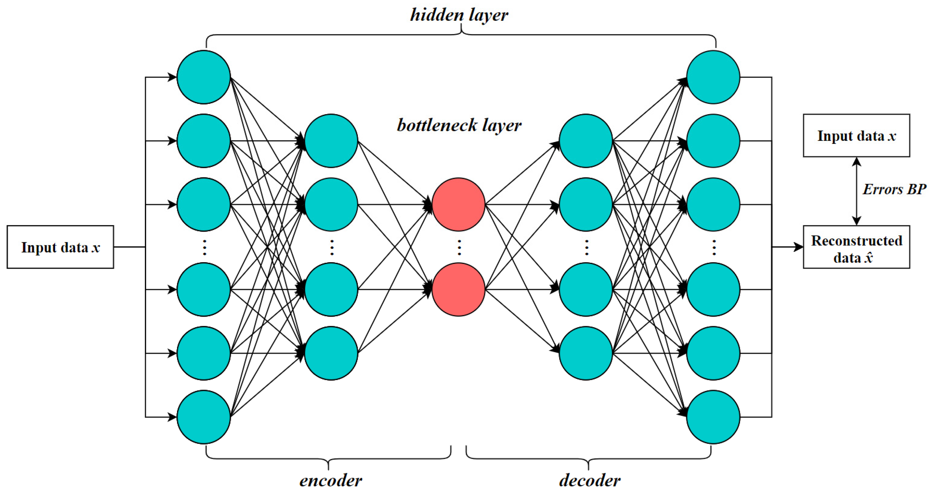
Deep autoencoder is an unsupervised neural network model composed of multiple layers of encoders and decoders. It is primarily used for learning low-dimensional representations (feature extraction) from unlabeled data while preserving the ability to reconstruct the input data [52]. Both the encoder and decoder are typically implemented using multilayer nonlinear neural networks (e.g., ReLU, sigmoid). Each layer progressively compresses the high-dimensional input into a more compact representation (encoding), and then reconstructs it layer by layer (decoding), allowing the model to extract more powerful nonlinear features compared to shallow autoencoders. The architecture is illustrated in Figure 2.
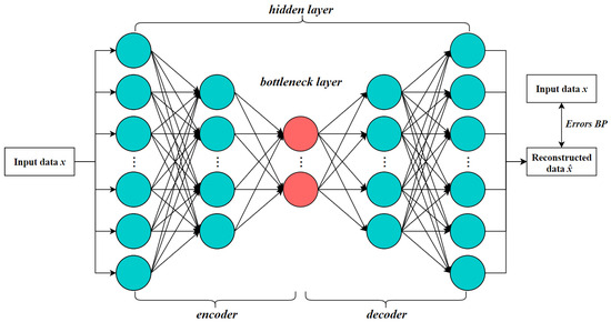
Figure 2.
Architecture of the deep autoencoder.
In hyperspectral unmixing tasks, the input layer receives the spectral vector x of a single pixel, which typically represents a mixed spectrum containing contributions from multiple endmembers. The encoder is responsible for learning the nonlinear interactions between endmembers and capturing structural features of the spectral curve. The bottleneck layer, also known as the latent space, represents the “mixing proportions”—that is, the abundance vector a, which simulates the abundance estimation process in nonlinear unmixing. The decoder reconstructs the mixed spectrum from the estimated abundances, effectively modeling the forward mixing process. The output layer produces a reconstructed spectrum , which is expected to closely approximate the original input x, thereby indicating the quality of the unmixing.
In addition, DAE-based unmixing methods typically employ the SoftMax activation function at the bottleneck layer to enforce abundance constraints, ensuring that the output satisfies both the ANC and the ASC. Sparse regularization is also introduced to promote the activation of only a few endmembers per pixel, thereby enhancing the interpretability of the unmixing results.
2.3. Channel Attention Module
Channel attention is a widely used attention mechanism in computer vision, primarily designed to capture the inter-channel dependencies of feature maps. It enables the network to focus more effectively on informative features by emphasizing important channels while suppressing less relevant ones [53]. In this mechanism, each channel of the feature map is treated as an independent feature detector that selectively responds to task-relevant information within the input.
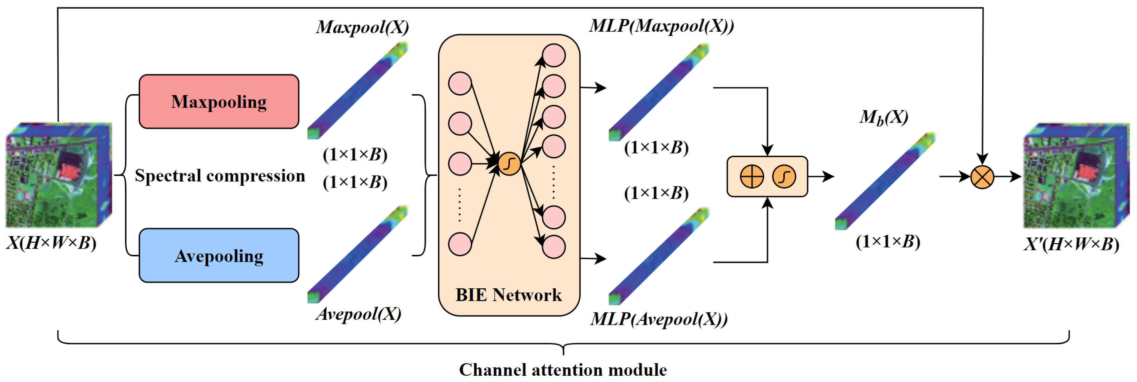
In hyperspectral unmixing tasks, the channel attention module automatically evaluates the importance of each spectral band in the input image and assigns corresponding weights, thereby enhancing the model’s discriminative capability. The structure is illustrated in Figure 3.

Figure 3.
Architecture of the Channel Attention Module (CAM).
Specifically, for a hyperspectral feature map , where B is the number of spectral bands, global max pooling and global average pooling are first performed along the spatial dimensions of each band to obtain two band descriptor vectors of size 1 × 1 × B. These vectors represent the maximum and average spatial responses of each band, reflecting their contribution to endmember characteristics. These two descriptors are then fed into a shared Band Importance Extraction Network (BIE Network), which consists of a two-layer Multilayer Perceptron (MLP). The first layer reduces the number of neurons to B/r (where r is the reduction ratio) and applies the ReLU activation function. The second layer restores the dimensionality back to B. The purpose of this MLP is to extract importance weights for each spectral band from the compressed statistical descriptors.
The outputs of the two MLP branches are then element-wise added and passed through a Sigmoid activation function to obtain a normalized band attention vector , which indicates the relative importance of each spectral band for the current unmixing task. This attention vector is then multiplied element-wise with the original hyperspectral feature map X, enhancing informative and discriminative bands while suppressing redundant or noisy ones. This process ultimately improves the accuracy of endmember identification and abundance estimation.
The channel attention computation can be summarized by the following formula:
Finally, the attention weight vector is element-wise multiplied with the original feature map, i.e., the hyperspectral image X, to obtain the channel-refined feature map X′ (H × W × B) after attention-based weighting:
where X′ represents the feature map after channel attention is applied, is the computed channel (band) attention vector, and ⊙ denotes element-wise multiplication.
2.4. Deep Residual Encoder
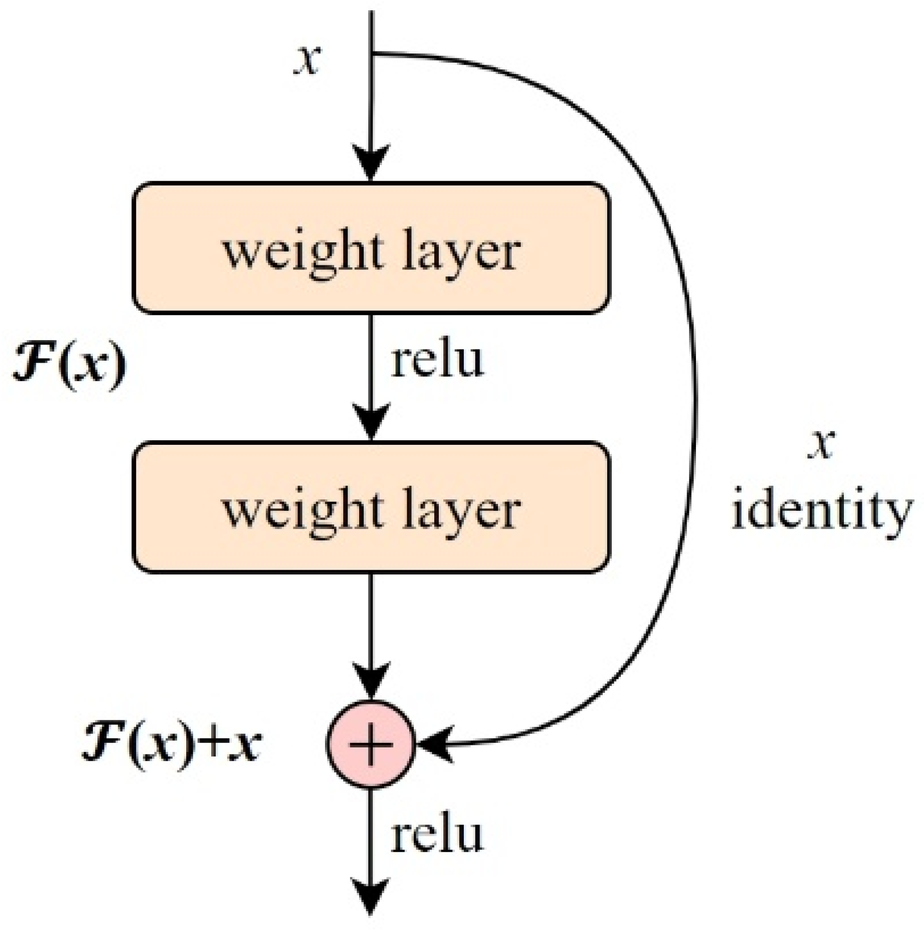
The Residual Encoder refers to a module embedded with residual connections [54] within the encoder structure, as shown in Figure 4. Its core idea is to allow the input to bypass intermediate nonlinear layers via skip connections and be directly added to the output, thereby alleviating training difficulties in deep networks, accelerating convergence, and mitigating the vanishing gradient problem. Assuming the input is x, and the internal residual mapping is a nonlinear transformation , the output of the residual block is:

Figure 4.
Residual connection module.
There, is typically composed of 1–3 linear (or convolutional) layers followed by activation functions; the input x bypasses the intermediate mapping and is added directly to . Activation functions (such as ReLU or LeakyReLU) can be placed either between layers or at the end. In hyperspectral unmixing tasks, where input spectra have high dimensionality and complex features (e.g., sparse mixing and nonlinear interference), introducing residual blocks can enhance the stability and representational power of abundance estimation and endmember separation. Especially when using MLP as the encoder, integrating Residual Encoder effectively mitigates network degradation and enables deeper networks to model complex mixing behaviors [55,56].
2.5. CResDAE Model Architecture
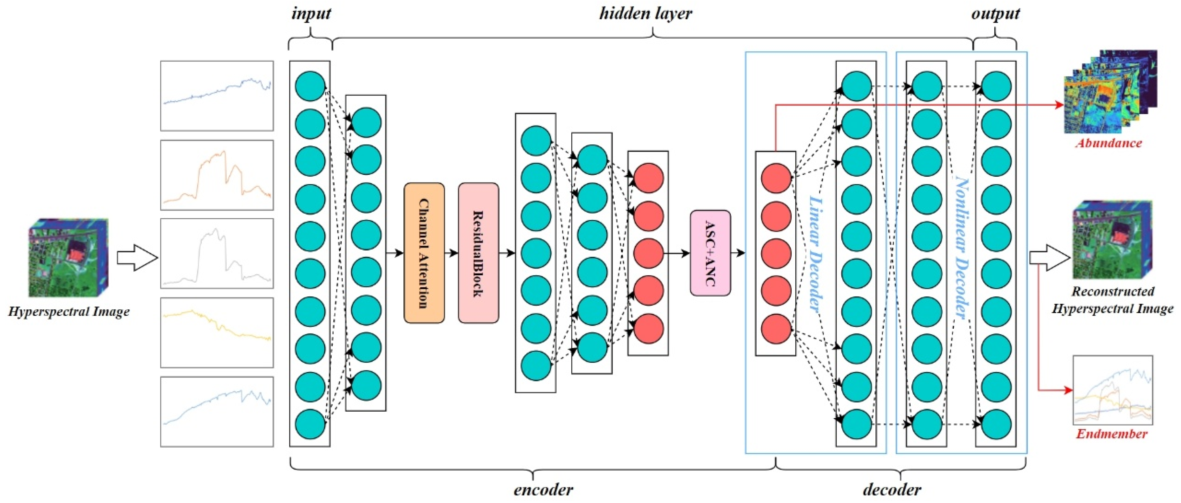
To adaptively assign different weights to spectral bands, enhance robustness against anomalies or noisy regions, improve nonlinear mapping capacity, and accelerate convergence, we introduce the Channel Attention Module and Residual Blocks into the deep autoencoder network, thereby proposing the CResDAE model. The overall architecture is shown in Figure 5.

Figure 5.
Architecture of the proposed CResDAE model.
Specifically, the encoder and decoder consist of a total of 14 layers—9 in the encoder and 5 in the decoder—including various types such as input layers, activation layers, hidden layers, and output layers, as detailed in Table 1 and Table 2. The encoder (layers 1–9) nonlinearly compresses high-dimensional input spectra into low-dimensional abundance coefficients through a series of fully connected layers and LeakyReLU activation functions. Embedded within it, a Channel Attention Module captures global spectral information via global average pooling and employs a bottleneck structure comprising dimensionality reduction (activated by ReLU) and restoration (activated by Sigmoid) to adaptively generate channel weights. This process recalibrates features toward key diagnostic spectral bands, significantly enhancing the model’s discriminative capability for spectral characteristics. Simultaneously, residual connections in the encoder effectively mitigate the vanishing gradient problem, ensuring stable training of the deep network. The decoder (layers 10–14) utilizes the estimated abundances, first passing through a linear layer to simulate linear spectral mixing, and then compensating for residuals via a path containing nonlinear hidden layers, ultimately reconstructing the original spectral signal with high precision. This design enables CResDAE to synergistically leverage both physics-driven and data-driven learning to jointly optimize the estimation of endmembers and abundances.

Table 1.
Encoder structure of the CResDAE model.

Table 2.
Decoder structure of the CResDAE model.
In addition, to balance spectral reconstruction accuracy with the physical interpretability of abundances and to enhance the overall accuracy and robustness of unmixing, we construct a composite loss function that integrates five constraints: reconstruction error, spectral angle similarity, sparsity, uniformity, and information entropy. The sparsity term helps suppress redundancy during early training, while the uniformity term regularizes the endmember distribution to prevent collapse. The loss function is formulated as follows:
Here, and are the weighting coefficients for each term.
- (1)
- Mean Squared Error (MSE) Loss: Measures the squared Euclidean distance between the reconstructed and the true spectra, reflecting numerical reconstruction accuracy [57].
: Original Spectral Pixel, : Reconstructed Spectral Pixel, : Number of Samples.
- (2)
- Spectral Angle Mapper (SAM) Loss: Measures the angle between the predicted and true spectra on the unit hypersphere, emphasizing spectral directional consistency [58].
Here a small constant (e.g., 1 × 10⁻⁸) is added to the denominator to prevent division by zero.
Uniform Loss: Encourages the overall abundance distribution to be uniform across all endmembers, preventing endmember collapse or underutilization [59].
: An all-ones vector of length K.
Entropy Loss: Encourages the abundance distribution to approach a one-hot form—sparse but not overly extreme—so as to avoid high uncertainty or excessive averaging in the model [60].
: Abundance of endmember k in pixel i, a small constant is added to prevent log(0).
In this model, in addition to reconstruction error and spectral angle similarity, the uniformity term plays a dominant role with a weighting coefficient of 0.4, while the sparsity and entropy terms are assigned coefficients of 0.01.
3. Data Acquisition and Processing
3.1. Urban Dataset
The Urban dataset is one of the most widely used hyperspectral datasets in hyperspectral unmixing research. It includes spectral signatures of ground objects, hyperspectral imagery, and ground truth data comprising endmembers and abundances. These components are used for generating synthetic hyperspectral data, training models, performing unmixing on real imagery, and evaluating unmixing results [61].
3.1.1. Urban Hyperspectral Image
The Urban hyperspectral image consists of 307 × 307 pixels, with each pixel representing an area of 2 × 2 square meters. A false-color composite image is shown in the figure. The image contains 210 spectral bands covering wavelengths from 400 nm to 2500 nm, with a spectral resolution of 10 nm. Due to the effects of dense water vapor absorption and atmospheric interference, bands 1–4, 76, 87, 101–111, 136–153, and 198–210 are removed, leaving 162 usable bands. The data is provided in .mat format.
3.1.2. Spectral Signatures of Ground Objects
The Urban dataset includes real-world spectra for several land cover types such as asphalt, grass, trees, rooftops, soil, and metal. Depending on the number of endmembers, versions of the dataset are available in 4-, 5-, and 6-endmember configurations. In this study, we adopt the 5-endmember version, which includes asphalt, grass, trees, rooftops, and soil, as shown in Figure 6.
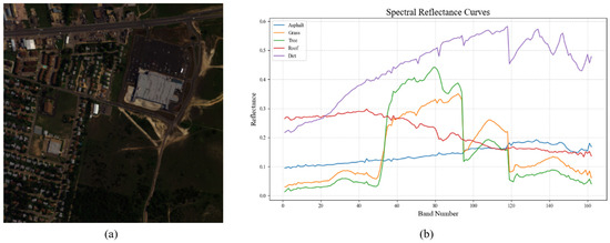
Figure 6.
(a) Urban hyperspectral image (b) Spectral signatures of five ground endmembers.
3.2. GF-5 Hyperspectral Data
The GF-5 satellite was successfully launched on 9 May 2018, and is the world’s first satellite capable of performing integrated observations of both land and atmosphere. It captures hyperspectral imagery with 330 spectral bands ranging from visible to shortwave infrared (400–2500 nm), with a spectral resolution of 5 nm in the visible range, a swath width of 60 km, and a spatial resolution of 30 m.
3.2.1. Hyperspectral Image of the Study Area
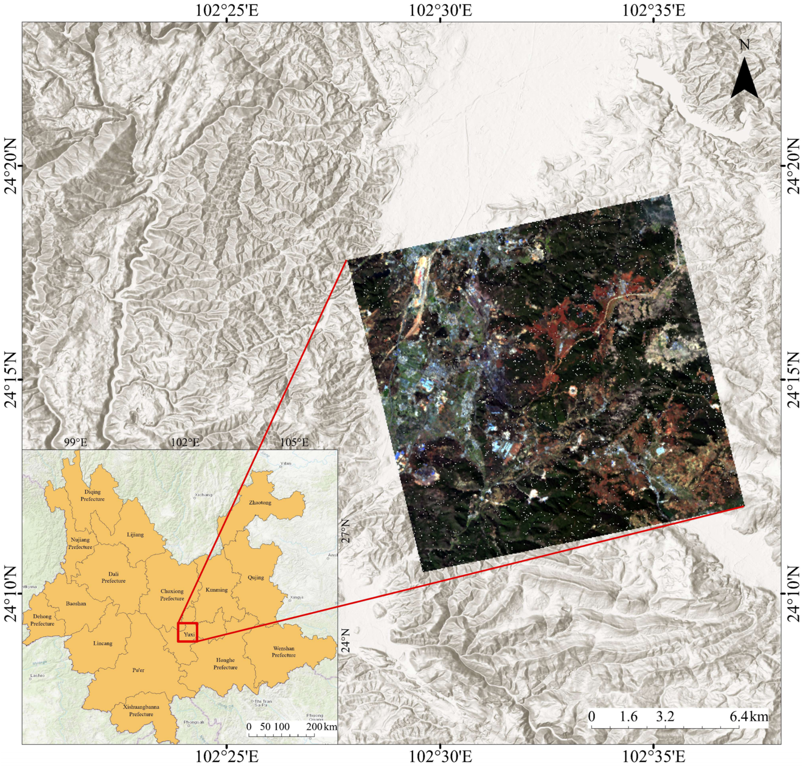
The study area is located in Yuxi City, Yunnan Province, China, approximately between 24°10′N−24°20′N and 102°25′E−102°40′E. The acquired GF-5 file is named: GF5_AHSI_E102.59_N24.38_20200212_009385_L10000072775. After a series of preprocessing steps—including radiometric calibration, atmospheric correction, orthorectification, and bad band removal (25 bands removed, leaving 305 bands)—a subregion rich in land cover diversity and spectral characteristics was selected and cropped to serve as the experimental image, as shown in Figure 7.
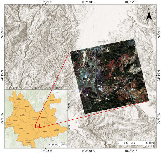
Figure 7.
GF-5 hyperspectral image of the study area.
3.2.2. Endmember Spectra of Surface Materials
Using ENVI 6.0 and its spectral identification tools, five types of ROI samples were selected from the hyperspectral image, corresponding to the following surface materials:
(1) Forest; (2) Grassland; (3) Layered silicate minerals (e.g., illite and sepiolite), which commonly represent materials such as weathered soil, exposed sediment zones, areas surrounding construction land, and regions of vegetation degradation in hyperspectral unmixing; (4) Carbonate minerals (e.g., dolomite and calcite), typically representing bare rock surfaces, quarries, construction material sites, or arid carbonate deposition zones; (5) Sulfate minerals (e.g., jarosite), which often indicate acidified bare soil, reddish surfaces, or abandoned mining/tailings areas.
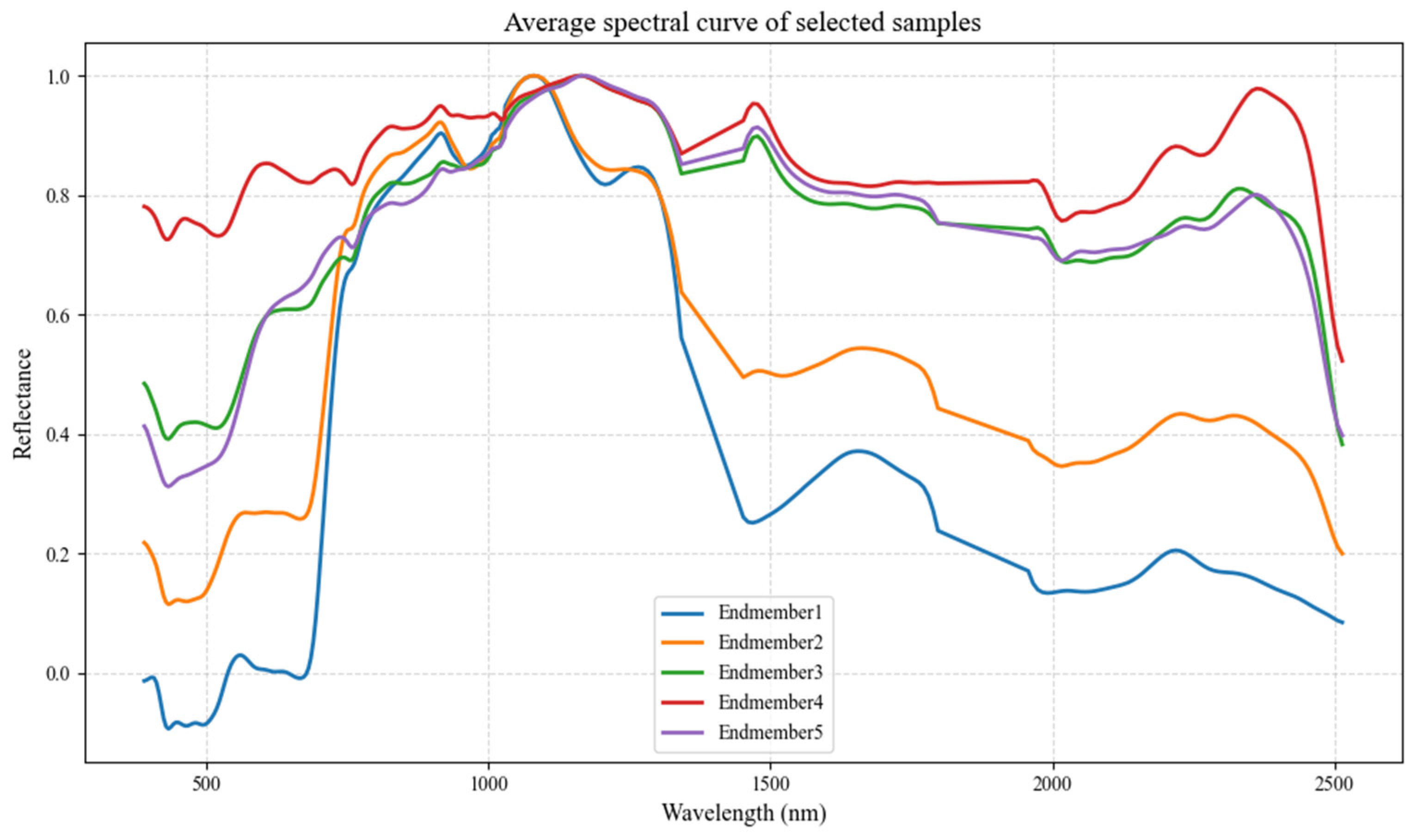
The average spectral signature of each ROI was extracted, and after removing water absorption bands (1350–1450 nm and 1800–1950 nm), followed by Gaussian smoothing and max normalization, the resulting endmember spectra were visualized as shown in Figure 8, corresponding to Endmembers 1 through 5.
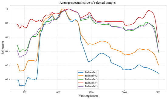
Figure 8.
Spectral curves of surface material endmembers.
4. Experiment
4.1. Construction of Simulated Hyperspectral Dataset
Using the Urban dataset as a reference for training, we constructed a simulated hyperspectral dataset based on a spectral library containing five endmembers: asphalt, grass, trees, rooftops, and soil. Datasets were generated under different signal-to-noise ratios (SNRs) of 10, 20, and 30 dB. Various mixing models—such as linear, bilinear, and post-nonlinear models—were applied, along with Gaussian filtering and normalization, to produce physically meaningful synthetic hyperspectral image cubes. The resulting dataset includes 3D hyperspectral data cubes and corresponding abundance maps, packaged into .mat files containing variables such as hyperspectral_cube, abundance_cube, mineral_names, spectra_library, wavelengths, SNR_dB, and mixing_model. The dataset structure and variable dimensions are illustrated in Figure 9.

Figure 9.
Structure of the synthetic dataset.
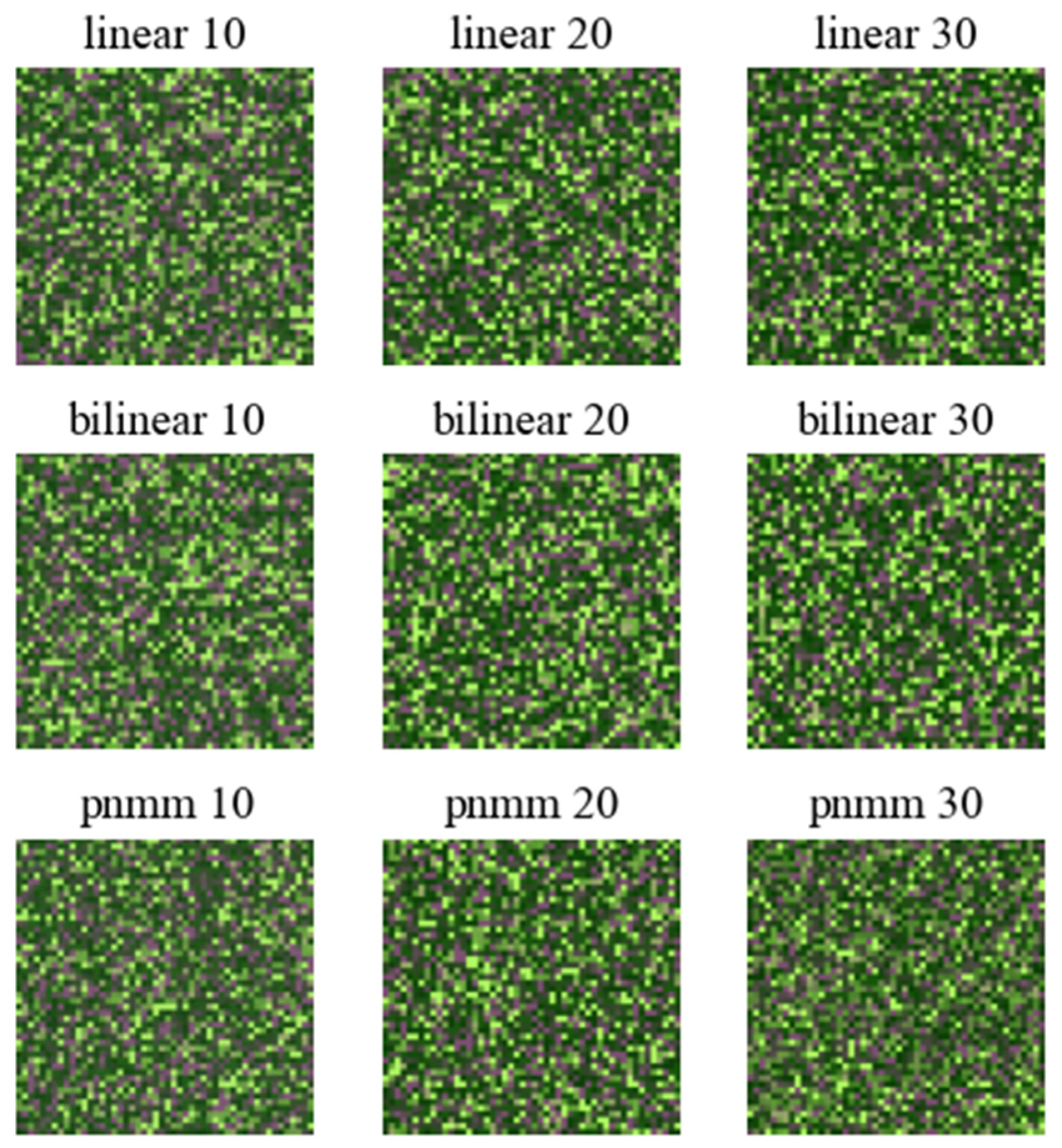
This dataset can be used for testing hyperspectral unmixing algorithms, as well as for model training and evaluation. Simulated false-color hyperspectral images with nine different combinations of mixing types and signal-to-noise ratios are shown in Figure 10.
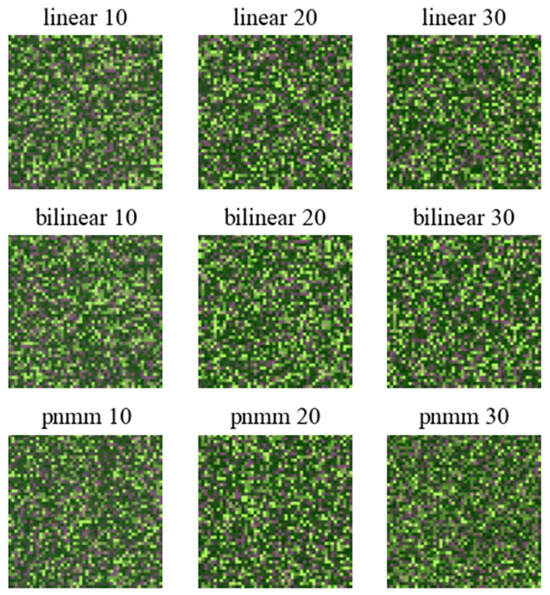
Figure 10.
False-color synthetic images of simulated hyperspectral data.
4.2. CResDAE Model Training
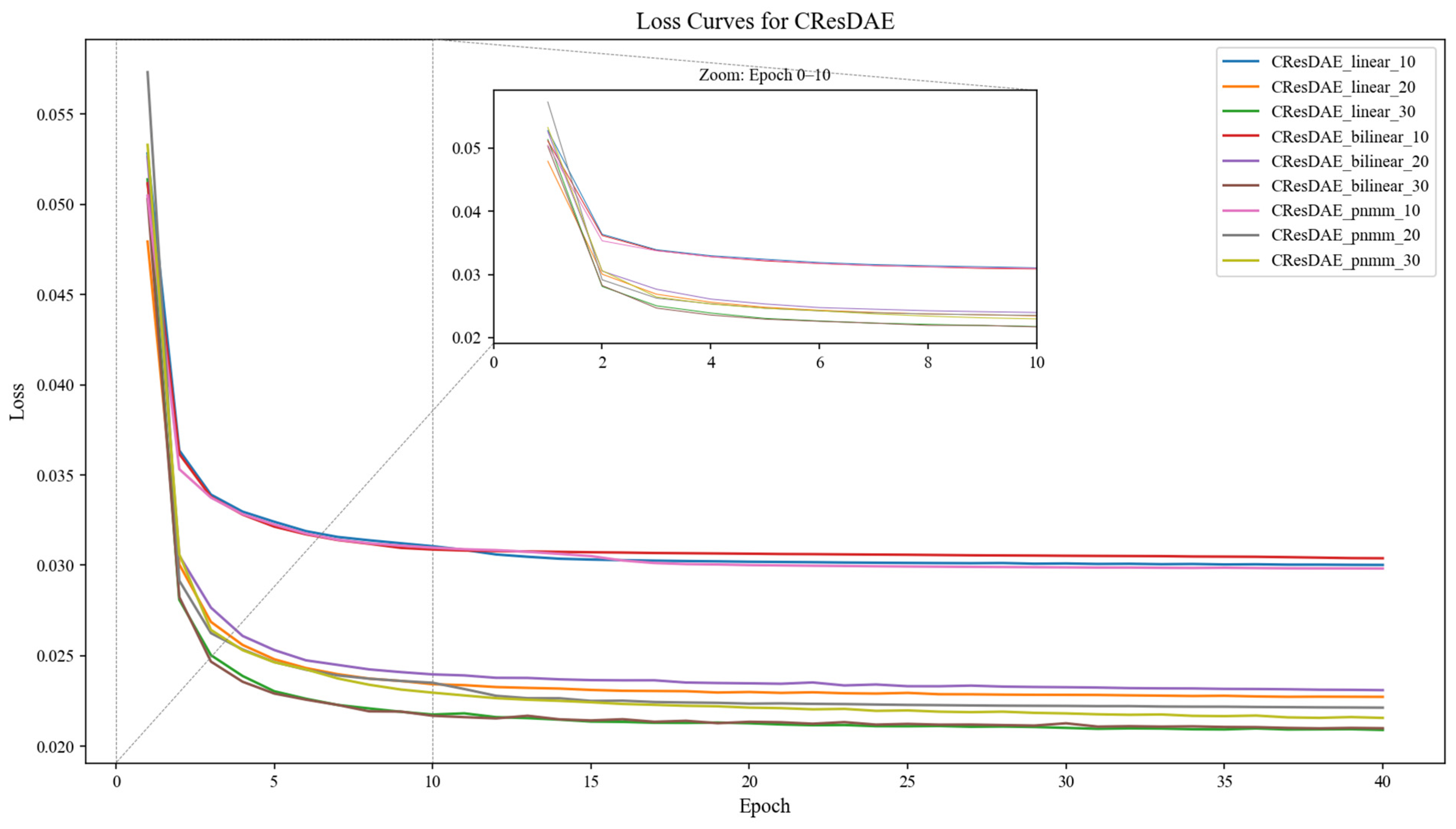
The CResDAE model was trained on a system equipped with an Intel® Core™ i7-14700KF CPU and an NVIDIA GeForce RTX 4060Ti 8 GB GPU, implemented using the PyTorch 2.6.0 framework. The Adam optimizer was employed to compute and update the neural network weights. The main network was trained with a learning rate of 1 × 10⁻³, while the pre-trained linear and nonlinear decoders were fine-tuned with a smaller learning rate of 1 × 10⁻⁵ to preserve structural priors. The model was trained with a batch size of 1024 over 40 epochs. A composite loss function was used, incorporating MSE, SAM, sparsity, uniformity, and entropy terms to constrain the model output from multiple perspectives. The nine synthetic hyperspectral datasets generated in Section 4.1 were used as training data in sequence. The training loss curves are shown in Figure 11. During training, the model outputs abundance maps (mixing proportions for each pixel) and endmember spectra (spectral signatures of components), and the trained model parameters were saved for each dataset.
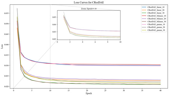
Figure 11.
Training loss curves of CResDAE on nine synthetic datasets.
4.3. Unmixing on Simulated Datasets and Multi-Model Evaluation
To validate the advantages of the proposed model, we compared it with several previously established mixed pixel decomposition methods or models. The models used for comparison include:
- (1)
- MVC-NMF (Minimum Volume Constrained Nonnegative Matrix Factorization): An extension of traditional NMF that introduces a minimum volume constraint (MVC) to reduce solution ambiguity and enhance the physical interpretability of the unmixing results [62,63].
- (2)
- VCA+K-Hype (Vertex Component Analysis + Kernel-based Hyperspectral Unmixing): This method extracts the purest pixels (vertices) as endmembers and maps the mixing process into a kernel space to better model nonlinear mixing effects [20,64,65].
- (3)
- LinearAE (Linear Autoencoder): A simple autoencoder structure in which the encoder output represents abundance, and the decoder performs a fixed linear combination of endmembers. It is suited for linear mixing scenarios [66].
- (4)
- ConvAE (Convolutional Autoencoder): This model treats hyperspectral images as spatial tensors and introduces convolutional layers to extract local features, enhancing the spatial continuity of abundance estimation [67].
- (5)
- NAE (Nonlinear Autoencoder): A deep nonlinear autoencoder that simultaneously models abundance estimation and nonlinear mixing through both encoder and decoder, making it well-suited for complex nonlinear scenarios [68,69].
Among the five comparison methods or models and our proposed CResDAE, MVC-NMF and VCA+K-Hype are unsupervised approaches that do not require training data; they perform unmixing directly on the dataset or image. In contrast, other deep learning-based unmixing models, such as those based on autoencoders (AE) or convolutional neural networks (CNN), are trained on simulated datasets while simultaneously performing unmixing, and they can be transferred to other datasets for further unmixing tasks.
For model evaluation, we selected four metrics to compare and assess model performance:
- (1)
- Root Mean Squared Error (RMSE): Measures the average Euclidean distance between the reconstructed spectra and the ground truth spectra after unmixing [70].
- (2)
- Spectral Angle Distance (SAD): Measures the angle between the estimated and ground truth spectra, reflecting their directional similarity. It is commonly used to assess spectral similarity at the endmember or pixel level. The unit is either radians or degrees—the smaller the value, the better the similarity [71].
- (3)
- Spectral Information Divergence (SID): An information-theoretic metric that quantifies the dissimilarity between two spectral vectors in terms of their probability distributions. A smaller value indicates higher spectral similarity [72].
- (4)
- Peak Signal-to-Noise Ratio (PSNR): Measures the fidelity of image or spectral reconstruction and is commonly used for quality assessment in image processing. A higher value indicates better reconstruction quality [73].
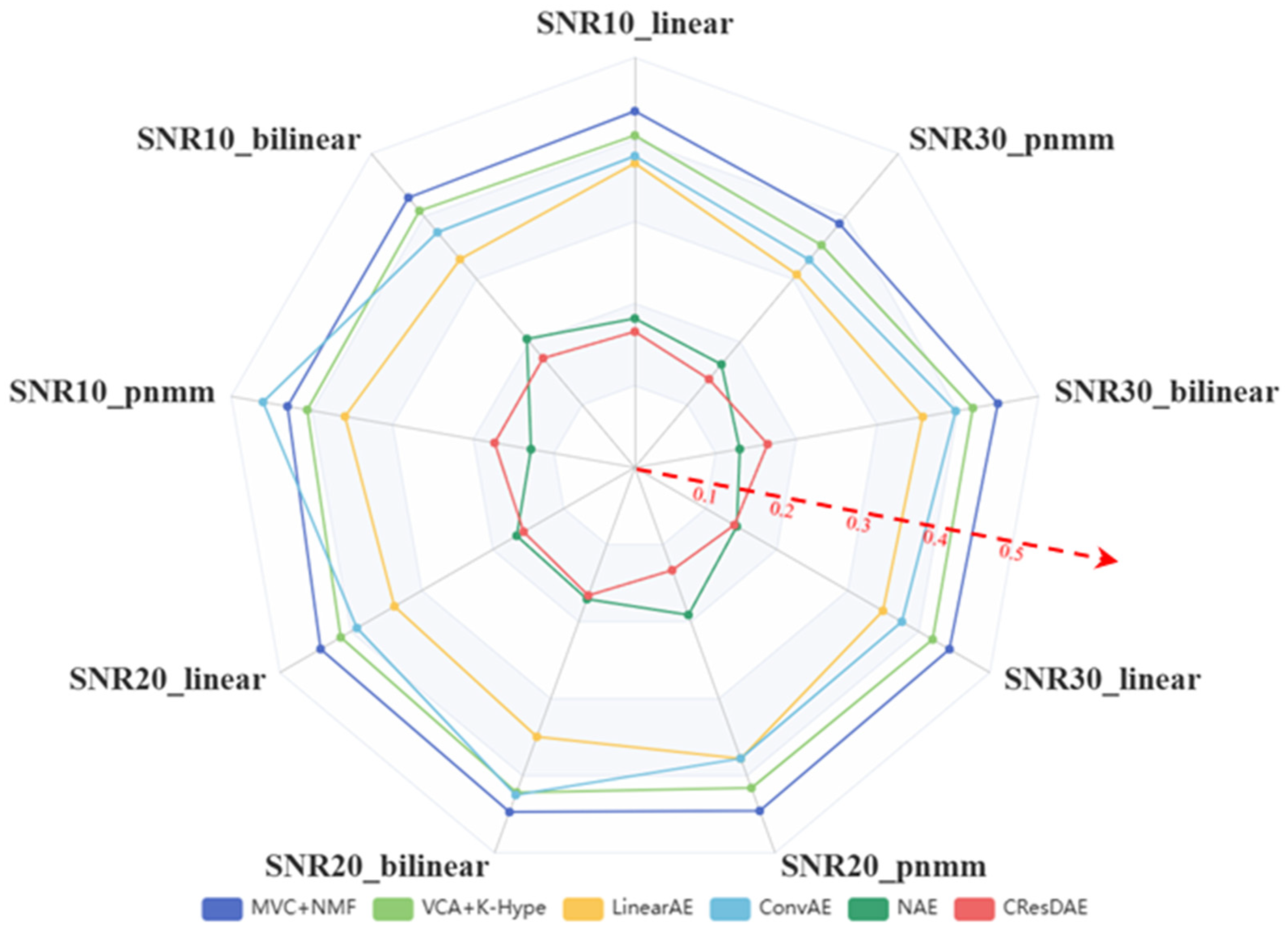
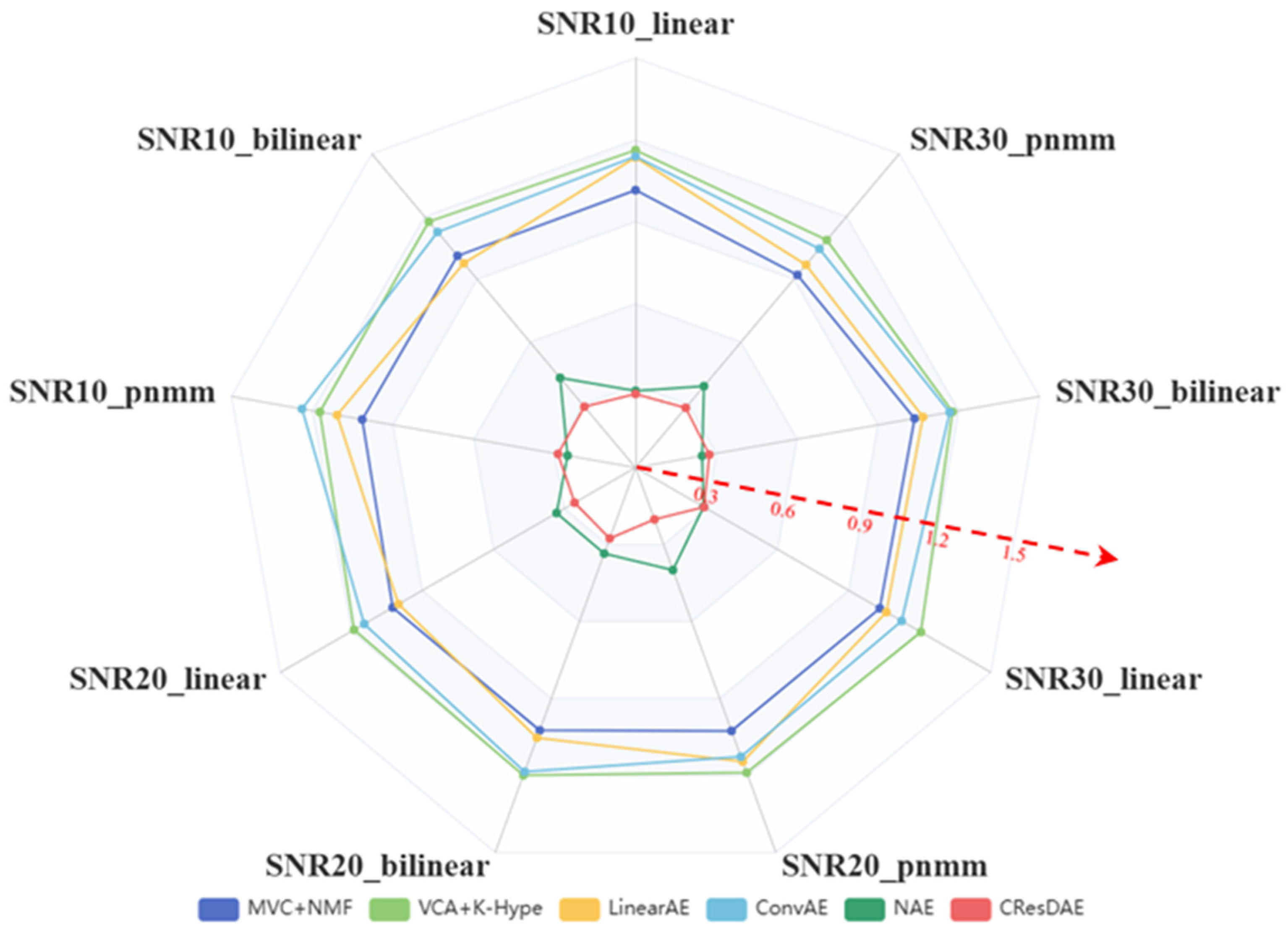
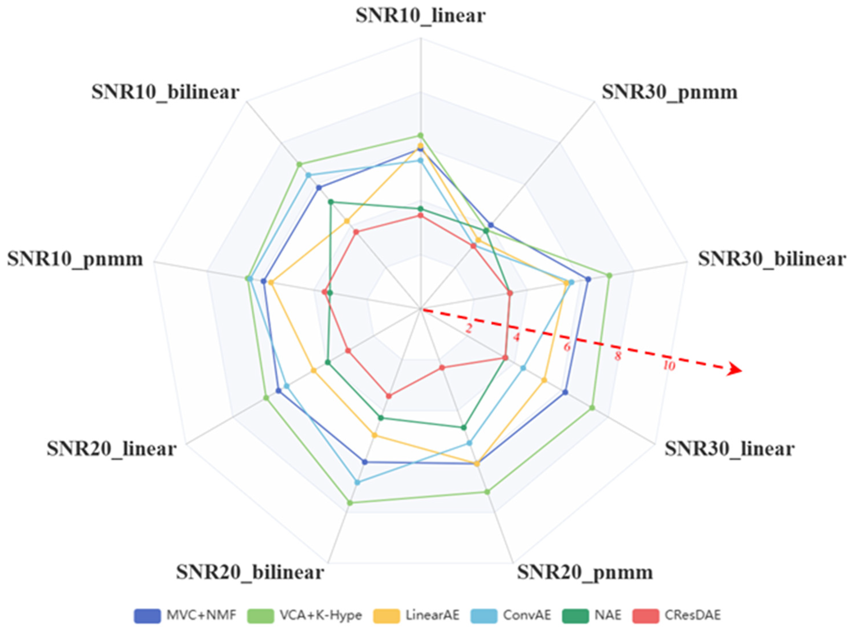
Next, we applied MVC-NMF, VCA+K-Hype, LinearAE, ConvAE, NAE, and the proposed CResDAE to perform unmixing on the simulated hyperspectral datasets and computed evaluation metrics. The RMSE results are presented in Table 3, SAD in Table 4, and SID in Table 5. Since the simulated datasets are artificially generated, PSNR is not used for assessing image quality.

Table 3.
RMSE comparison across different models.

Table 4.
SAD comparison across different models.

Table 5.
SID comparison across different models.
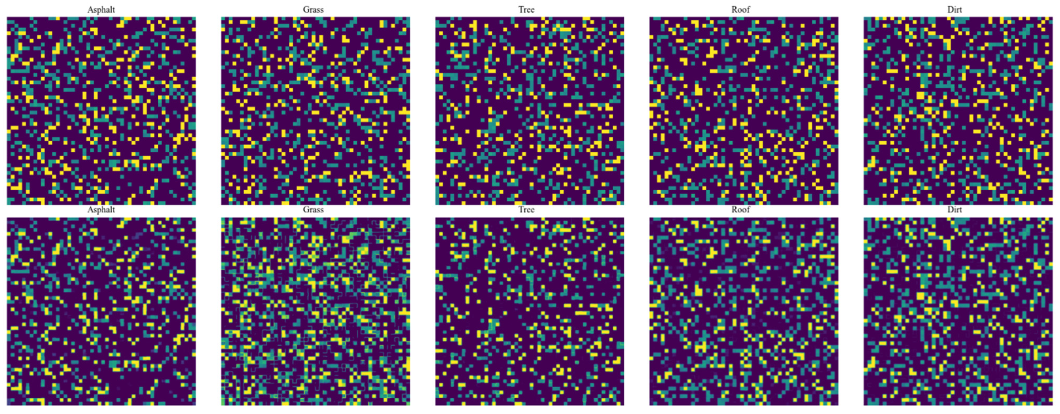
To enhance the comparative effect of the indicators, the visualizations are shown in Figure 12, Figure 13 and Figure 14. By comparing the calculation results of the evaluation indicators, it is evident that the proposed CResDAE model achieves the best overall performance in mixed pixel decomposition on the synthetic hyperspectral datasets. It consistently demonstrates superior abundance estimation accuracy and competitive endmember extraction performance across both linear and nonlinear mixing scenarios. A visual example of the unmixing performance of CResDAE on one dataset is shown in Figure 15.
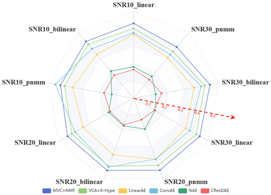
Figure 12.
RMSE comparison across different models.
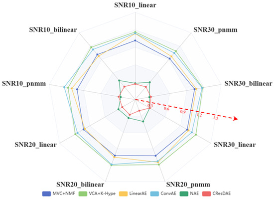
Figure 13.
SAD comparison across different models.

Figure 14.
SID comparison across different models.

Figure 15.
Unmixing results under PNMM mixing model with SNR = 20 ((top): real, (bottom): predicted).
4.4. Urban Data Unmixing
Based on the unmixing performance and evaluation metrics presented in Section 4.3, both in tables and figures, the Nonlinear Autoencoder (NAE) emerged as the best-performing model aside from the proposed CResDAE. Therefore, we selected NAE and CResDAE for further unmixing experiments on the Urban hyperspectral dataset. The Urban image was loaded into both models using their respective trained weight files to perform abundance estimation. The resulting abundance maps and endmember spectral curves for each land cover type were obtained. The ground truth abundance maps for the Urban scene are shown in Figure 16. According to different mixing models, the estimated results and their corresponding endmember spectra are compared against the ground truth and visualized in Figure 17, Figure 18, Figure 19, Figure 20, Figure 21 and Figure 22.

Figure 16.
Ground truth abundance maps of the Urban dataset.

Figure 17.
Abundance map comparison under linear mixing at different SNRs ((Left): NAE, (Right): CResDAE).

Figure 18.
Unmixing spectral curve comparison under linear mixing at different SNRs ((Left): NAE, (Right): CResDAE).

Figure 19.
Abundance map comparison under bilinear mixing at different SNRs ((Left): NAE, (Right): CResDAE).

Figure 20.
Unmixing spectral curve comparison under bilinear mixing at different SNRs ((Left): NAE, (Right): CResDAE).

Figure 21.
Abundance map comparison under pnmm mixing at different SNRs ((Left): NAE, (Right): CResDAE).

Figure 22.
Unmixing spectral curve comparison under pnmm mixing at different SNRs ((Left): NAE, (Right): CResDAE).
As shown in Figure 17, Figure 19 and Figure 21, the proposed model is capable of producing clear and spatially coherent abundance maps under various mixing models and SNR conditions, indicating strong nonlinear unmixing capabilities. Moreover, the endmember spectral curves in Figure 18, Figure 20 and Figure 22 exhibit high similarity to the true endmembers, further validating the model’s endmember extraction performance. Across all mixing models and SNR settings, CResDAE consistently demonstrates clearer and more distinct unmixing and inversion results compared to NAE, confirming the superior effectiveness of the proposed model. In addition, we conducted a comprehensive comparison between NAE and CResDAE by calculating the overall RMSE, class-wise RMSE, SAD, SID, and PSNR for the unmixing results. The quantitative results are summarized in Table 6 and Table 7.

Table 6.
Unmixing performance of NAE on the Urban dataset.

Table 7.
Unmixing performance of CResDAE on the Urban dataset.
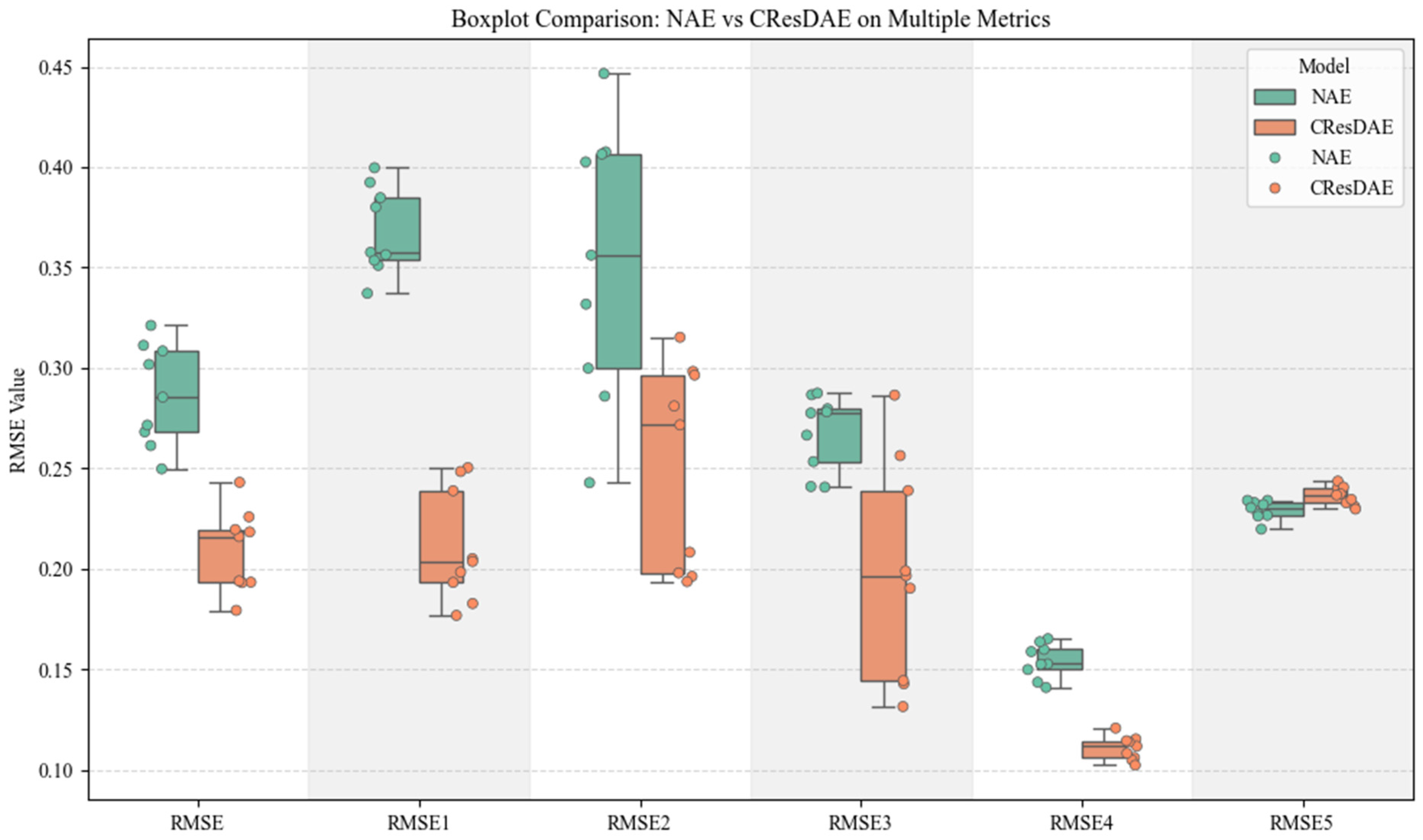
The visual comparison of the two tables and the RMSE box plot (as shown in Figure 23) reveals that CResDAE achieves lower RMSE values than NAE for all land cover types except the fifth one, where it is slightly higher. This again demonstrates that the proposed CResDAE model places greater emphasis on generalization and robustness under complex material mixing conditions, showcasing its potential and practical value in real-world hyperspectral unmixing applications.

Figure 23.
Box plot of RMSE comparison between the two models.
4.5. Unmixing of GF-5 Hyperspectral Imagery
To comprehensively evaluate the performance of the CResDAE model, we conducted systematic unmixing experiments and multi-model comparisons on both the simulated dataset (Section 4.2) and the Urban standard dataset (Section 4.3). Experimental results demonstrate that CResDAE excels in both endmember extraction and abundance inversion. This superior performance stems primarily from its innovative channel attention mechanism and deep residual encoding module. These components synergistically enhance the model’s ability to capture and model complex, diverse spectral features of land cover objects, thereby significantly improving its adaptability and robustness across different regions and scenarios.
Based on the above validation, we applied the trained CResDAE model to deconvolve real GF-5 hyperspectral imagery (Section 3.2.1). The specific workflow (as shown in Figure 1) is as follows: First, initial endpoints are extracted from the GF-5 imagery itself (Section 3.2.2); Then, these endpoints are used to synthesize simulated data for fine-tuning the pre-trained model; finally, the optimized model performs full-scene unmixing on the entire GF-5 image. The resulting abundance maps for different land cover types, shown in Figure 24, exhibit clear and reasonable spatial distributions. Figure 25 further compares the spectral curves of land cover types obtained through model unmixing with those extracted from the original image, revealing high consistency in absorption characteristics and waveforms. Collectively, these results demonstrate that CResDAE achieves outstanding pixel-level deconvolution and abundance inversion performance on real GF-5 data.

Figure 24.
Abundance maps generated by CResDAE on the GF-5 hyperspectral image (a) Forest; (b) Grassland; (c) Layered silicate minerals; (d) Carbonate minerals; (e) Sulfate minerals.

Figure 25.
Endmember spectral curves estimated by CResDAE on the GF5 hyperspectral image.
4.6. Discussion
Based on the comparative experiments and evaluation metrics in Section 4.3 and Section 4.4, it is evident that CResDAE outperforms other methods and models, including MVC-NMF, VCA+K-Hype, LinearAE, ConvAE, and NAE. Specifically, across all mixing models and SNR levels, CResDAE achieves an average reduction of 0.1919 in RMSE, 0.6726 in SAD, and 2.0995 in SID.
This improvement is primarily attributed to the enhanced model architecture:
- Channel Attention Mechanism significantly improves the model’s sensitivity to critical mineral spectral regions by assigning higher weights to key spectral positions (e.g., mineral absorption peaks), while suppressing noise and redundant bands. This allows the model to effectively distinguish endmembers even when their reflectance spectra are very similar.
- Deep Residual Structure mitigates training degradation and enhances feature expressiveness, helping to avoid performance drops in deeper networks and improving both convergence speed and training stability.
- Nonlinear Skip Connections enable the model to handle common nonlinear mixing effects observed in real-world scenarios. This structure allows the model to approximate bilinear interactions and can be extended to more complex forms such as exponential mixing models (e.g., PNMM).
The combined effect of these components allows CResDAE to outperform both traditional methods and basic neural network architectures in hyperspectral unmixing tasks under complex conditions.
In the comparison between NAE and CResDAE, we observed that CResDAE achieves an average RMSE of 0.2092, representing a 27.01% improvement over NAE’s 0.2866. Furthermore, SAD, SID, and PSNR were improved by 37.39%, 40.79%, and 25.24%, respectively. These results suggest that: The introduction of the attention mechanism helps retain more spectral shape information; Residual connections contribute significantly to suppressing high-frequency noise; The overall spatial structure of the reconstructed images remains well-preserved. Among the five land cover types, only the last category, “soil,” exhibited a higher RMSE in CResDAE compared to NAE. This discrepancy may be attributed to the spectral characteristics of soil, which often exhibit high variability or strong inter-class spectral mixing in hyperspectral images. Soil reflectance spectra typically show moderate intensity and gradual transitions, but in the Urban dataset, soil pixels frequently coexist with man-made surfaces (e.g., road edges) or sparse vegetation. In such moderately complex spectra, NAE’s simpler structure may favor conservative reconstruction, leading to lower RMSE. In contrast, CResDAE, with its enhanced nonlinear expressiveness, performs well for most endmembers, but may amplify local spectral fluctuations in boundary mixtures or low-proportion endmembers, potentially increasing RMSE in those cases. We plan to mitigate or eliminate this issue by introducing multi-scale feature fusion, enhancing spatial-channel joint attention, and incorporating adversarial training/domain adaptation techniques.
In the simulated data experiments, a comprehensive evaluation of the unmixing performance under known ground truth conditions was conducted by comparing several representative methods, including MVC-NMF, VCA+K-Hype, LinearAE, ConvAE, NAE, and the proposed CResDAE. These methods encompass both traditional linear and nonlinear unmixing algorithms as well as mainstream deep learning-based models, thereby providing a well-rounded performance benchmark. In contrast, the real hyperspectral image experiments involved a comparison between only NAE and CResDAE. This selection was based on two main considerations: first, the lack of accurate abundance ground truth in real remote sensing scenarios limits the reliability of quantitative evaluations for traditional methods; second, as a state-of-the-art nonlinear autoencoder-based unmixing model, NAE is representative and provides a meaningful baseline, which highlights the generalization capability and interpretability of CResDAE under complex real-world material distributions. Therefore, this experimental setup emphasizes assessing the practical value of the model in real geological environments.
In Section 4.5, the application of CResDAE to real GF-5 hyperspectral imagery for mixed pixel decomposition and mineral abundance estimation demonstrates the following:
- (1)
- Application Potential and Practical Value in Real Environments: In field experiments using GF-5 hyperspectral imagery from Yunnan, the CResDAE model exhibited strong unmixing capability and robustness. It was able to stably extract endmember spectra and their spatial distributions even under complex and variable natural surface conditions.
- (2)
- Sensitivity to Endmember Proportion and High-Abundance Regions: CResDAE demonstrated high sensitivity to fine-grained variations in endmember proportions (as seen in Figure 24), effectively capturing gradual transitions in boundary regions rather than abrupt changes. In particular, it accurately revealed the cross-distribution of layered silicates and sulfates, reflecting spatial patterns of material migration and surface weathering.
- (3)
- Interpretability under Semi-Supervised Conditions: Under semi-supervised learning conditions—guided by only a limited number of ROI samples—CResDAE extracted endmember spectra that closely matched the mean spectral curves of the ROIs, indicating strong interpretability.
- (4)
- Suitability for Complex Surface Environments: The abundance estimation method of CResDAE is well-suited for fine-grained modeling in areas with complex terrain and coexisting or overlapping materials, addressing the limitations of traditional classification and spectral identification methods in handling mixed pixels.
- (5)
- Application Value in Mineral Exploration and Potential in Vegetated Areas: The results demonstrate that CResDAE can transform hyperspectral imagery into environmental and geological information maps with high reliability, supporting field geological surveys and remote sensing-based mineral exploration. For example: Abundance maps can help identify mineral-enriched zones (e.g., carbonate anomalies), serving as remote sensing indicators of alteration zones; Unmixing results can assist in constructing mineral assemblage layers (e.g., carbonate + muscovite/illite + clay-type indicator minerals) for anomaly zone delineation; When overlaid with existing geological maps, the analysis can significantly narrow the scope and reduce the cost of field investigations.
Furthermore, CResDAE shows resistance to vegetation interference, enabling it to extract non-vegetation components in vegetated areas. When combined with NDVI or vegetation masks, it can enhance unmixing performance for mineral endmembers beneath vegetation cover.
In summary, despite demonstrating strong performance in hyperspectral unmixing tasks, CResDAE still faces significant challenges in geological applications: On one hand, the model exhibits limited capability in identifying minerals within areas of dense vegetation cover, where vegetation spectra severely obscure underlying mineralization information; On the other hand, inherent difficulties in geological unmixing—such as uncertainty in the number of mineral endpoints, spectral variability caused by “same substance, different spectra,” and domain shifts resulting from differences in land cover across regions—constrain the model’s accuracy and generalization capability. To address these challenges, future research may integrate vegetation endpoint constraints and incorporate multi-source hyperspectral data, transfer learning, or domain adaptation techniques to mitigate domain shift [74,75]. Concurrently, combining mineral spectral library priors or geological constraints to guide endpoint extraction could enhance the model’s adaptability and practicality in complex geological environments, particularly in identifying mineral anomalies within dense forest regions.
5. Conclusions
Through the construction of simulated hyperspectral datasets, a series of training, unmixing, and comparison experiments under various models, datasets, mixing types, and signal-to-noise ratios, as well as real-data application on GF-5 imagery, we draw the following conclusions:
- (1)
- The proposed CResDAE model introduces a channel attention mechanism and deep residual structure into the hyperspectral unmixing framework. This enhances the model’s ability to assign adaptive weights to spectral bands in geological unmixing tasks and equips the abundance estimation network with nonlinear skip connections. As a result, the model achieves improved nonlinear modeling capacity and spectral feature responsiveness, demonstrating superior robustness and generalization across both synthetic and real hyperspectral datasets.
- (2)
- Experimental results show that CResDAE consistently outperforms traditional and other deep learning-based methods. It exhibits notably better decoupling performance and spatial continuity, especially in boundary regions of mixed pixels. Compared with MVC + NMF, VCA+K-Hype, LinearAE, ConvAE, and NAE on synthetic datasets, CResDAE achieves average improvements of 0.1919 in RMSE, 0.6726 in SAD, and 2.0995 in SID. On the Urban dataset, compared to NAE, RMSE improves by 27.01%, while SAD, SID, and PSNR improve by 37.39%, 40.79%, and 25.24%, respectively.
- (3)
- In the real-data experiments on GF-5 hyperspectral imagery from the Yunnan region, the proposed CResDAE model demonstrates strong adaptability for cross-regional land cover recognition. It effectively distinguishes forest, grassland, silicate, carbonate, and sulfate materials across different areas. The extracted endmember spectral curves exhibit high interpretability, and the spatial distribution of the abundance maps shows strong consistency with actual surface cover. These results provide high-confidence data support for field geological surveys and remote sensing-based mineral exploration, offering decision-making references and technical assistance for geological prospecting in covered regions.
Author Contributions
Conceptualization, C.Z., J.W., K.Z., Q.Q., G.Q. and D.L.; methodology, C.Z., D.L., H.Q. and C.L.; validation, C.Z.; formal analysis, C.Z.; investigation, C.Z., J.B. and Q.Z.; resources, J.W. and K.Z.; data curation, C.Z., W.W. and T.L.; writing—original draft preparation, C.Z.; writing—review and editing, J.W.; supervision, J.W., J.B. and K.Z.; project administration, J.W.; funding acquisition, J.W., W.W. and J.B. All authors have read and agreed to the published version of the manuscript.
Funding
This work was supported by the Third Xinjiang Scientific Expedition Program under Grant No. 2022xjkk1306, and the Strategic Priority Research Program of the Chinese Academy of Sciences under Grant No. XDA0430103.
Data Availability Statement
The original contributions presented in the study are included in the article, further inquiries can be directed to the corresponding author.
Conflicts of Interest
The authors declare no conflicts of interest.
References
- Tong, Q.X.; Zhang, B.; Zheng, L.F. Hyperspectral Remote Sensing; Higher Education Press: Beijing, China, 2006; pp. 1–3. [Google Scholar]
- Qian, S.E. Hyperspectral satellites, evolution, and development history. IEEE J. Sel. Top. Appl. Earth Obs. Remote Sens. 2021, 14, 7032–7056. [Google Scholar] [CrossRef]
- Li, J.; Zheng, K.; Gao, L.; Han, Z.; Li, Z.; Chanussot, J. Enhanced Deep Image Prior for Unsupervised Hyperspectral Image Super-Resolution. IEEE Trans. Geosci. Remote Sens. 2025, 63, 5504218. [Google Scholar] [CrossRef]
- Li, J.; Zheng, K.; Gao, L.; Ni, L.; Huang, M.; Chanussot, J. Model-Informed Multistage Unsupervised Network for Hyperspectral Image Super-Resolution. IEEE Trans. Geosci. Remote Sens. 2024, 62, 5516117. [Google Scholar] [CrossRef]
- Liu, C.; Xing, C.; Hu, Q.; Wang, S.; Zhao, S.; Gao, M. Stereoscopic hyperspectral remote sensing of the atmospheric environment: Innovation and prospects. Earth-Sci. Rev. 2022, 226, 103958. [Google Scholar] [CrossRef]
- Ang, K.L.M.; Seng, J.K.P. Big data and machine learning with hyperspectral information in agriculture. IEEE Access 2021, 9, 36699–36718. [Google Scholar] [CrossRef]
- Nisha, A.; Anitha, A. Current advances in hyperspectral remote sensing in urban planning. In Proceedings of the 2022 Third International Conference on intelligent computing instrumentation and control technologies (ICICICT), Kannur, India, 11–12 August 2022; IEEE: Piscataway, NJ, USA, 2022; pp. 94–98. [Google Scholar]
- Qasim, M.; Khan, S.D.; Haider, R.; Rasheed, M.U. Integration of multispectral and hyperspectral remote sensing data for lithological mapping in Zhob Ophiolite, Western Pakistan. Arab. J. Geosci. 2022, 15, 599. [Google Scholar] [CrossRef]
- Chakraborty, R.; Kereszturi, G.; Pullanagari, R.; Durance, P.; Ashraf, S.; Anderson, C. Mineral prospecting from biogeochemical and geological information using hyperspectral remote sensing-Feasibility and challenges. J. Geochem. Explor. 2022, 232, 106900. [Google Scholar] [CrossRef]
- Li, D.; Chen, S.; Chen, X. Research on method for extracting vegetation information based on hyperspectral remote sensing data. Trans. CSAE 2010, 26, 181–185, (In Chinese with English Abstract). [Google Scholar]
- Chen, J.; Ma, L.; Chen, X.H.; Rao, Y.H. Research progress of spectral mixture analysis. J. Remote Sens. 2016, 20, 1102–1109, (In Chinese with English Abstract). [Google Scholar] [CrossRef]
- Bioucas-Dias, J.M.; Plaza, A.; Dobigeon, N.; Parente, M.; Du, Q.; Gader, P.; Chanussot, J. Hyperspectral unmixing overview: Geometrical, statistical, and sparse regression-based approaches. IEEE J. Sel. Top. Appl. Earth Obs. Remote Sens. 2012, 5, 354–379. [Google Scholar] [CrossRef]
- Zhang, B.; Sun, X. Hyperspectral Images Unmixing Algorithm; Science Press: Beijing, China, 2015. [Google Scholar]
- Borsoi, R.A.; Imbiriba, T.; Bermudez, J.C.M.; Richard, C.; Chanussot, J.; Drumetz, L.; Tourneret, J.Y.; Zare, A.; Jutten, C. Spectral variability in hyperspectral data unmixing: A comprehensive review. IEEE Geosci. Remote Sens. Mag. 2021, 9, 223–270. [Google Scholar] [CrossRef]
- Guerra, R.; Santos, L.; López, S.; Sarmiento, R. A new fast algorithm for linearly unmixing hyperspectral images. IEEE Trans. Geosci. Remote Sens. 2015, 53, 6752–6765. [Google Scholar] [CrossRef]
- Campos, S.P. Linear Spectral Mixing Model: Theoretical Concepts, Algorithms and Applications of Studies in the Legal Amazon. Rev. Bras. Cartogr. 2020, 72, 50. [Google Scholar]
- Dobigeon, N.; Tourneret, J.Y.; Richard, C.; Bermudez, J.C.M.; McLaughlin, S.; Hero, A.O. Nonlinear unmixing of hyperspectral images: Models and algorithms. IEEE Signal Process. Mag. 2013, 31, 82–94. [Google Scholar] [CrossRef]
- Heylen, R.; Parente, M.; Gader, P. A review of nonlinear hyperspectral unmixing methods. IEEE J. Sel. Top. Appl. Earth Obs. Remote Sens. 2014, 7, 1844–1868. [Google Scholar] [CrossRef]
- Winter, M.E. N-FINDR: An algorithm for fast autonomous spectral end-member determination in hyperspectral data. In Imaging spectrometry V; SPIE: Bellingham, WA, USA, 1999; Volume 3753, pp. 266–275. [Google Scholar]
- Nascimento, J.M.; Dias, J.M. Vertex component analysis: A fast algorithm to unmix hyperspectral data. IEEE Trans. Geosci. Remote Sens. 2005, 43, 898–910. [Google Scholar] [CrossRef]
- Iordache, M.D.; Bioucas-Dias, J.M.; Plaza, A. Sparse unmixing of hyperspectral data. IEEE Trans. Geosci. Remote Sens. 2011, 49, 2014–2039. [Google Scholar] [CrossRef]
- Zhou, Y.; Rangarajan, A.; Gader, P.D. A Gaussian mixture model representation of endmember variability in hyperspectral unmixing. IEEE Trans. Image Process. 2018, 27, 2242–2256. [Google Scholar] [CrossRef]
- Lee, D.D.; Seung, H.S. Learning the parts of objects by non-negative matrix factorization. Nature 1999, 401, 788–791. [Google Scholar] [CrossRef]
- Zhou, G.; Xie, S.; Yang, Z.; Yang, J.M.; He, Z. Minimum-volume-constrained nonnegative matrix factorization: Enhanced ability of learning parts. IEEE Trans. Neural Netw. 2011, 22, 1626–1637. [Google Scholar] [CrossRef]
- Palsson, F.; Sigurdsson, J.; Sveinsson, J.R.; Ulfarsson, M.O. Neural network hyperspectral unmixing with spectral information divergence objective. In Proceedings of the 2017 IEEE International Geoscience and Remote Sensing Symposium (IGARSS), Fort Worth, TX, USA, 23–28 July 2017; IEEE: Piscataway, NJ, USA, 2017; pp. 755–758. [Google Scholar]
- Deshpande, V.S.; Bhatt, J.S. A practical approach for hyperspectral unmixing using deep learning. IEEE Geosci. Remote Sens. Lett. 2021, 19, 5511505. [Google Scholar]
- Dong, H.; Zhang, X.; Zhang, J.; Meng, H.; Jiao, L. Graph-based Adaptive Network with Spatial-Spectral Features for Hyperspectral Unmixing. IEEE J. Sel. Top. Appl. Earth Obs. Remote Sens. 2025, 18, 12865–12881. [Google Scholar] [CrossRef]
- Zhao, X.; Ma, J.; Wang, L.; Zhang, Z.; Ding, Y.; Xiao, X. A review of hyperspectral image classification based on graph neural networks. Artif. Intell. Rev. 2025, 58, 172. [Google Scholar] [CrossRef]
- Ghosh, P.; Roy, S.K.; Koirala, B.; Rasti, B.; Scheunders, P. Hyperspectral unmixing using transformer network. IEEE Trans. Geosci. Remote Sens. 2022, 60, 5535116. [Google Scholar] [CrossRef]
- Duan, Y.; Xu, X.; Li, T.; Pan, B.; Shi, Z. UnDAT: Double-aware transformer for hyperspectral unmixing. IEEE Trans. Geosci. Remote Sens. 2023, 61, 5522012. [Google Scholar] [CrossRef]
- Jin, Z.; Yi, X.; Liu, Y.; Zhang, H. Multilinear hyperspectral unmixing based on autoencoder and recurrent neural network. Appl. Soft Comput. 2025, 185, 113972. [Google Scholar] [CrossRef]
- Alshahrani, A.A.; Bchir, O.; Ben Ismail, M.M. Autoencoder-Based Hyperspectral Unmixing with Simultaneous Number-of-Endmembers Estimation. Sensors 2025, 25, 2592. [Google Scholar] [CrossRef]
- Wan, L.; Chen, T.; Plaza, A.; Cai, H. Hyperspectral unmixing based on spectral and sparse deep convolutional neural networks. IEEE J. Sel. Top. Appl. Earth Obs. Remote Sens. 2021, 14, 11669–11682. [Google Scholar] [CrossRef]
- Yu, Y.; Ma, Y.; Mei, X.; Fan, F.; Huang, J.; Li, H. Multi-stage convolutional autoencoder network for hyperspectral unmixing. Int. J. Appl. Earth Obs. Geoinf. 2022, 113, 102981. [Google Scholar] [CrossRef]
- Wang, J.; Xu, J.; Chong, Q.; Liu, Z.; Yan, W.; Xing, H.; Xing, Q.; Ni, M. SSANet: An adaptive spectral–spatial attention autoencoder network for hyperspectral unmixing. Remote Sens. 2023, 15, 2070. [Google Scholar] [CrossRef]
- Qu, Y.; Qi, H. uDAS: An untied denoising autoencoder with sparsity for spectral unmixing. IEEE Trans. Geosci. Remote Sens. 2018, 57, 1698–1712. [Google Scholar] [CrossRef]
- Li, J.; Zheng, K.; Li, Z.; Gao, L.; Jia, X. X-Shaped Interactive Autoencoders with Cross-Modality Mutual Learning for Unsupervised Hyperspectral Image Super-Resolution. IEEE Trans. Geosci. Remote Sens. 2023, 61, 5518317. [Google Scholar] [CrossRef]
- Yu, X.C.; Xiong, L.P.; Xu, J.D. Mineral mapping based on secondary scattering mixture model. Remote Sens. Land Resour. 2014, 26, 60–68. [Google Scholar]
- Ozkan, S.; Kaya, B.; Akar, G.B. Endnet: Sparse autoencoder network for endmember extraction and hyperspectral unmixing. IEEE Trans. Geosci. Remote Sens. 2018, 57, 482–496. [Google Scholar] [CrossRef]
- Su, Y.; Marinoni, A.; Li, J.; Plaza, J.; Gamba, P. Stacked nonnegative sparse autoencoders for robust hyperspectral unmixing. IEEE Geosci. Remote Sens. Lett. 2018, 15, 1427–1431. [Google Scholar] [CrossRef]
- Bedini, E. The use of hyperspectral remote sensing for mineral exploration: A review. J. Hyperspectral Remote Sens. 2017, 7, 189–211. [Google Scholar] [CrossRef]
- Lin, H.L.; Zhang, X.; Sun, Y.L. Hyperspectral sparse unmixing of minerals with single scattering albedo. J. Remote Sens. 2016, 20, 53–61. [Google Scholar] [CrossRef]
- Peyghambari, S.; Zhang, Y. Hyperspectral remote sensing in lithological mapping, mineral exploration, and environmental geology: An updated review. J. Appl. Remote Sens. 2021, 15, 031501. [Google Scholar] [CrossRef]
- Attallah, Y.; Zigh, E.; Adda, A.P. Optimized 3D-2D CNN for automatic mineral classification in hyperspectral images. Rep. Geod. Geoinformatics 2024, 118, 82–91. [Google Scholar] [CrossRef]
- Zhang, X.; Xing, W.U.; Honglei, L.I.N.; Nan, W.A.N.G. Retrieval of mineral abundances of delta region in Eberswalde, Mars. Natl. Remote Sens. Bull. 2021, 22, 304–312. [Google Scholar]
- Zhao, P.; Chen, Y. Digital geology and quantitative mineral exploration. Earth Sci. Front. 2021, 28, 1. [Google Scholar]
- Cheng, Q.; Gao, M. Comparative Studies of Nonlinear Models and Their Applications to Magmatic Evolution and Crustal Growth of the Huai’an Terrane in the North China Craton. Fractal Fract. 2025, 9, 38. [Google Scholar] [CrossRef]
- Li, C.; Zhou, K.; Gao, W.; Luo, X.; Tao, Z.; Liu, P.; Qiu, W. Geochemical prospectivity mapping using compositional balance analysis and multifractal modeling: A case study in the Jinshuikou area, Qinghai, China. J. Geochem. Explor. 2024, 257, 107361. [Google Scholar] [CrossRef]
- Zuo, R.; Yang, F.; Cheng, Q.; Kreuzer, O.P. A novel data-knowledge dual-driven model coupling artificial intelligence with a mineral systems approach for mineral prospectivity mapping. Geology 2025, 53, 284–288. [Google Scholar] [CrossRef]
- Heylen, R.; Scheunders, P. A multilinear mixing model for nonlinear spectral unmixing. IEEE Trans. Geosci. Remote Sens. 2015, 54, 240–251. [Google Scholar] [CrossRef]
- Altmann, Y.; Dobigeon, N.; Tourneret, J.Y. Unsupervised post-nonlinear unmixing of hyperspectral images using a Hamiltonian Monte Carlo algorithm. IEEE Trans. Image Process. 2014, 23, 2663–2675. [Google Scholar] [CrossRef]
- Hinton, G.E.; Salakhutdinov, R.R. Reducing the dimensionality of data with neural networks. Science 2006, 313, 504–507. [Google Scholar] [CrossRef]
- Woo, S.; Park, J.; Lee, J.Y.; Kweon, I.S. Cbam: Convolutional block attention module. In Proceedings of the European conference on computer vision (ECCV), Munich, Germany, 8–14 September 2018; pp. 3–19. [Google Scholar]
- He, K.; Zhang, X.; Ren, S.; Sun, J. Deep residual learning for image recognition. In Proceedings of the IEEE conference on computer vision and pattern recognition, Las Vegas, NV, USA, 27–30 June 2016; pp. 770–778. [Google Scholar]
- Zeng, Y.; Ritz, C.; Zhao, J.; Lan, J. Attention-based residual network with scattering transform features for hyperspectral unmixing with limited training samples. Remote Sens. 2020, 12, 400. [Google Scholar] [CrossRef]
- Yang, X.; Chen, J.; Wang, C.; Chen, Z. Residual dense autoencoder network for nonlinear hyperspectral unmixing. IEEE J. Sel. Top. Appl. Earth Obs. Remote Sens. 2022, 15, 5580–5595. [Google Scholar] [CrossRef]
- Haykin, S. Neural Networks and Learning Machines, 3rd ed.; Pearson Education: London, UK, 2009. [Google Scholar]
- Kruse, F.A.; Lefkoff, A.B.; Boardman, J.W.; Heidebrecht, K.B.; Shapiro, A.T.; Barloon, P.J.; Goetz, A.F.H. The spectral image processing system (SIPS)—Interactive visualization and analysis of imaging spectrometer data. Remote Sens. Environ. 1993, 44, 145–163. [Google Scholar] [CrossRef]
- Palsson, B.; Sigurdsson, J.; Sveinsson, J.R.; Ulfarsson, M.O. Hyperspectral Unmixing Using a Neural Network Autoencoder. IEEE Access 2018, 6, 25646–25656. [Google Scholar] [CrossRef]
- Shannon, C.E. A mathematical theory of communication. Bell Syst. Tech. J. 1948, 27, 379–423. [Google Scholar] [CrossRef]
- Sigurdsson, J.; Ulfarsson, M.O.; Sveinsson, J.R. Semi-supervised hyperspectral unmixing. In Proceedings of the 2014 IEEE Geoscience and Remote Sensing Symposium, Quebec City, QC, Canada, 13–18 July 2014; IEEE: Piscataway, NJ, USA, 2014. [Google Scholar]
- Jia, S.; Qian, Y. Constrained nonnegative matrix factorization for hyperspectral unmixing. IEEE Trans. Geosci. Remote Sens. 2008, 47, 161–173. [Google Scholar] [CrossRef]
- Nus, L.; Miron, S.; Brie, D. Estimation of the regularization parameter of an on-line NMF with minimum volume constraint. In Proceedings of the 2018 IEEE 10th Sensor Array and Multichannel Signal Processing Workshop (SAM), Sheffield, UK, 8–11 July 2018; IEEE: Piscataway, NJ, USA, 2018. [Google Scholar]
- Heinz, D.C.; Chang, C.I. Fully constrained least squares linear spectral mixture analysis method for material quantification in hyperspectral imagery. IEEE Trans. Geosci. Remote Sens. 2001, 39, 529–545. [Google Scholar] [CrossRef]
- Chen, J.; Richard, C.; Honeine, P. A novel kernel-based nonlinear unmixing scheme of hyperspectral images. In Proceedings of the 2011 Conference Record of the Forty Fifth Asilomar Conference on Signals, Systems and Computers (ASILOMAR), Pacific Grove, CA, USA, 6–9 November 2011; IEEE: Piscataway, NJ, USA, 2011; pp. 1898–1902. [Google Scholar][Green Version]
- Cronjaeger, C.; Pattison, R.C.; Tsay, C. Tensor-Based Autoencoder Models for Hyperspectral Produce Data. In Computer Aided Chemical Engineering; Elsevier: Amsterdam, The Netherlands, 2022; Volume 49, pp. 1585–1590. [Google Scholar]
- Ji, D.J.; Park, J.; Cho, D.H. ConvAE: A new channel autoencoder based on convolutional layers and residual connections. IEEE Commun. Lett. 2019, 23, 1769–1772. [Google Scholar] [CrossRef]
- Wang, M.; Zhao, M.; Chen, J.; Rahardja, S. Nonlinear unmixing of hyperspectral data via deep autoencoder networks. IEEE Geosci. Remote Sens. Lett. 2019, 16, 1467–1471. [Google Scholar] [CrossRef]
- Zhang, J.; Zhang, X.; Meng, H.; Sun, C.; Wang, L.; Cao, X. Nonlinear unmixing via deep autoencoder networks for generalized bilinear model. Remote Sens. 2022, 14, 5167. [Google Scholar] [CrossRef]
- Hastie, T.; Tibshirani, R.; Friedman, J. The Elements of Statistical Learning: Data Mining, Inference, and Prediction, 2nd ed.; Springer: New York, NY, USA, 2009. [Google Scholar]
- Dennison, P.E.; Halligan, K.Q.; Roberts, D.A. A comparison of error metrics and constraints for multiple endmember spectral mixture analysis and spectral angle mapper. Remote Sens. Environ. 2004, 93, 359–367. [Google Scholar] [CrossRef]
- Chang, C.-I. An information-theoretic approach to spectral variability, similarity, and discrimination for hyperspectral image analysis. IEEE Trans. Inf. Theory 2000, 46, 1927–1932. [Google Scholar] [CrossRef]
- Netravali, A.N. Digital Pictures: Representation, Compression, and Standards; Springer: Berlin/Heidelberg, Germany, 2013. [Google Scholar]
- Tuia, D.; Persello, C.; Bruzzone, L. Domain Adaptation for the Classification of Remote Sensing Data: An Overview of Recent Advances. IEEE Geosci. Remote Sens. Mag. 2016, 4, 41–57. [Google Scholar] [CrossRef]
- Baghbaderani, R.K.; Qu, Y.; Qi, H. Unsupervised Hyperspectral Image Domain Adaptation through Unmixing-Based Domain Alignment. In Proceedings of the IGARSS 2023–2023 IEEE International Geoscience and Remote Sensing Symposium, Pasadena, CA, USA, 16–21 July 2023; pp. 5906–5909. [Google Scholar]
Disclaimer/Publisher’s Note: The statements, opinions and data contained in all publications are solely those of the individual author(s) and contributor(s) and not of MDPI and/or the editor(s). MDPI and/or the editor(s) disclaim responsibility for any injury to people or property resulting from any ideas, methods, instructions or products referred to in the content. |
© 2025 by the authors. Licensee MDPI, Basel, Switzerland. This article is an open access article distributed under the terms and conditions of the Creative Commons Attribution (CC BY) license (https://creativecommons.org/licenses/by/4.0/).


