Highlights
What are the main findings?
- The classification accuracy of vegetation varied with images at different spatial resolution.
- Vegetation complexity affected classification accuracy.
What are the implications of the main findings?
- Mapping tidal marshes with different vegetation complexities should use images of different spatial resolutions.
- UAV data with 5 cm resolution was recommended for tidal marsh vegetation classification in the Yellow River Delta or regions of similar vegetation complexity.
Abstract
Unmanned aerial vehicle (UAV) images have increasingly become important data for accurate mapping of tidal marsh vegetation. They are particularly important for determining what spatial resolution is needed because UAV imaging requires a trade-off between spatial resolution and imaging extent. However, there are still insufficient studies for assessing the effects of spatial resolution on the classification accuracy of tidal marsh vegetation. This study utilized UAV images with spatial resolutions of 2 cm, 5 cm, and 10 cm, respectively, to classify seven tidal marsh plots with different vegetation complexities in the Yellow River Delta (YRD), China, using the object-oriented example-based feature extraction with support vector machine approach and the pixel-based random forest classifier, and compared the differences in vegetation classification accuracy. This study indicated the following: (1) Vegetation classification varied at different spatial resolutions, with a difference of 0.95–8.76% between the highest and lowest classification accuracy for different plots. (2) Vegetation complexity influenced classification accuracy. Classification accuracy was lower when the relative dominance and proportional abundance of P. australis and T. chinensis were higher in the plots. (3) Considering the trade-off between classification accuracy and imaging extent, UAV data with 5 cm spatial resolution were recommended for tidal marsh vegetation classification in the YRD or similar vegetation complexity regions.
1. Introduction
Tidal marshes are among the most productive ecosystems of the biosphere, composed of the diverse vegetation communities at the stressful transitional zones between land and sea [1,2,3], and support multiple ecosystem services such as biodiversity conservation, carbon sink, water quality improvement, shoreline protection, construction of tidal channel networks, reduction of flood risk, primary production, and climate change mitigation [4,5,6,7], which are greatly decided by the composition and structure of tidal marsh vegetation [8].
Tidal marshes can be mapped using remotely sensed techniques, and a globally consistent 10 m spatial resolution map of the world’s tidal marsh distribution for the year 2020 has been produced using Sentinel-1 and Sentinel-2 satellite data [9], which will help stakeholders to better comprehend the location and extent of tidal marshes, and to determine priority areas for conservation and restoration from a global to a regional perspective. However, it is necessary to map tidal marsh vegetation at a finer scale for monitoring and assessing the status, processes, and trends of the tidal marsh ecosystem, and proposing adaptive restoration strategies for tidal marshes and monitoring their progress [3,8,10]. Tidal marsh vegetation is highly sensitive to physical processes in tidal marsh landscapes. Vegetation composition, structure, and spatial distribution will vary with different salinity conditions in tidal marshes [11,12]. In particular, in the slow-flat areas of tidal marshes, a difference in horizontal distance of a few meters and a difference in altitude of only a few centimeters to a few decimeters can create very different water-salt environments [13], thus increasing the heterogeneity of the tidal marsh vegetation distribution [14], which makes it difficult to identify tidal marsh vegetation in imagery with a spatial resolution of less than 30 m [3,12].
The use of airborne and satellite images with spatial resolution better than 5 m and unmanned aerial vehicle (UAV) images at centimeter-scale spatial resolution has increased over the last two decades, becoming an important data source for identifying tidal marsh vegetation communities [15]. A 3 m spatial resolution map of tidal marsh vegetation communities with classification overall accuracy (OA) of 94% for high tidal marsh in the northeastern United States, including high marsh, low marsh, mudflat, phragmites, pool/panne, open water, terrestrial border, and upland, was produced using a random forest (RF) classifier and 3 m spatial resolution digital airborne ortho-photography with red, green, blue, and near-infrared bands [3]. Multispectral 10 cm UAV imagery with the RF method was used to classify a plant community of coastal meadows in West Estonia into reed swamp, lower shore, upper shore, open pioneer, and tall grass with a classification accuracy of a Fleiss’ kappa coefficient of 0.89 [8]. Multispectral 10 cm UAV imagery with the object-oriented example-based feature extraction with support vector machine approach (OEFESVM) was used to classify the vegetation community of mudflat areas in the Yellow River Delta (YRD), China, into Suaeda salsa (S. salsa), Suaeda salsa + Limonium bicolor [Bunge] Kuntze (S. salsa + L. bicolor), Tamarix chinensis (T. chinensis), Phragmites australis (P. australis), and non-vegetation with an OA of 95.0% [14]. Multispectral 2.5 cm UAV imagery with an object-oriented U-net method was utilized to classify plant species of coastal wetlands in the Mingjiang River estuary of South China into Kandelia candel, P. australis, Ipomoea pescaprae, Scirpus mariqueter, and Cyperus malaccensis with an OA of 95.7% [16]. Although classification OA in most studies was better than 80%, the user accuracy (UA) and producer accuracy (PA) of some vegetation communities were between 60% and 70%, and need to be further investigated.
In summary, the classification accuracy of tidal marsh vegetation is mainly related to the spectral and spatial resolution of remote sensing images and vegetation community types, while the choice of classification approach is of less importance, which is generally consistent with the viewpoint obtained from previous remote sensing identification of tree species [17]. By comparing the spectral and spatial resolution of several airborne and satellite images, it was concluded that spatial resolution was most important in salt marsh vegetation classification [18].
It is particularly important to determine what spatial resolution is needed for the identification of complex and diverse tidal marsh vegetation communities. However, there is still a lack of research on how spatial resolution affects the accuracy of vegetation classification in complex and diverse tidal marsh ecosystems [10,19]. Although UAV surveys can image with higher temporal and spatial resolution, more feasibility, and less expense [20,21], most current UAVs do not have a function of a priori configuration of optimum flight parameters, and the users struggle with the trade-off between spatial resolution (also called ground sampling distance) and imaging extent [22,23]. Logically, one UAV flight (same battery capacity) acquires high spatial resolution images with a relatively small imaging area, providing more detailed information on an interesting object [22]. For the same imaging extent, a higher spatial resolution means a higher flight time duration, more battery consumption, a greater number of images acquired, more storage space required, and a longer time to process the images, showing an exponential increase [21,22,24]. Therefore, the main issue to be dealt with is to ensure the appropriate spatial resolution of the UAV imagery required to complete mapping of specific tidal marsh vegetation communities, which is particularly crucial for users with limited time and budgets, such as fellow researchers and ecological monitors in nature reserves. Although studies have emerged to automatically estimate optimal UAV flight parameters [23], determining the appropriate spatial resolution remains a challenge for the identification of complex and diverse tidal marsh vegetation communities, which can reach the expectations of local managers in term of both classification accuracy and ecological significance.
Within global tidal marsh ecosystems, those located in the YRD of China support the migratory birds from Northeast Asia and the Western Pacific Rim to transfer, breed, and overwinter [25], and were included as a Ramsar Wetland of International Importance in 2013 and a World Natural Heritage Site in 2024. In the YRD, wetland restoration projects have been implemented continuously since 2002 and have achieved good results, but the wetland restoration area had low vegetation diversity and a single habitat type, which was prone to degradation once freshwater replenishment was stopped [26,27]. Therefore, it is essential to map the accurate composition and structure of tidal marsh vegetation to support the development of nature-based solutions to carry out effective management and scientific restoration projects [14,28]. Although some studies have been conducted on tidal marsh vegetation classification using various spatial resolutions of UAV multispectral data [14,29], it is still unclear what spatial resolution is more appropriate.
The overall aim of this study was to compare and evaluate the effects of the different spatial resolution UAV images on the classification accuracy of tidal marsh vegetation within multi-type plots with different vegetation complexities, and determine the appropriate spatial resolution of the UAV imagery for fine-scale mapping of vegetation communities over the region of interest in the YRD, China.
2. Materials and Methods
2.1. Study Area
UAV surveys were made in a slow-flat area of the northwestern Yiqianer Management Station, Dongying City, Shandong Province, China (Figure 1). The study area is occupied by sparse vegetation patches and bare mudflats. The vegetation cover and diversity decreased substantially from the north shoreline to the southern mudflats [14]. The vegetation has been previously classified as four communities [14]: S. salsa, S. salsa + L. bicolor, T. chinensis, and P. australis, plus non-vegetation type (including bare mudflats, water, and road). The May 2024 field survey validated this vegetation community classification. This study area was chosen because it is relatively natural and has not been impacted by human activities, except for the impact of land occupation by the construction of wind power, and no wetland restoration projects have been undertaken.
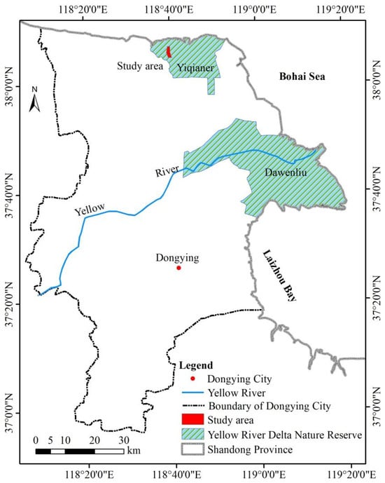
Figure 1.
Location of the study area within the Yiqianer Management Station in Dongying City, Shandong Province, China.
2.2. Image Acquisition and Processing
Multispectral images were acquired on 1–2 November 2023, in late fall, by a DJI Phantom 4 Multispectral UAV (DJI Sciences and Technologies Ltd., Shenzhen, China), with a built-in real-time DJITM Onboard D-RTK, providing centimeter-level positioning accuracy [14,30]. The DJI Phantom 4 Multispectral UAV contains six 1/2.9-inch CMOS sensors, including an RGB camera for visible light imaging and five monochrome sensors for multispectral imaging. The spectral sunlight sensor on top of the UAV can detect the solar irradiance in real time for image compensation (DJI Sciences and Technologies Ltd., Shenzhen, China). For more details, please refer to the DJI Phantom 4 Multispectral Quick Start Guide on the official DJI website (https://www.dji.com). The field survey was concurrently conducted, just as S. salsa was red, T. chinensis was green, P. australis was turning yellow, and L. bicolor was blooming with small, white and yellow flowers, at a time when the differences in color made them easy to identify. Field observations revealed that some of T. chinensis in the study area had a canopy size of less than 50 cm, and some of L. bicolor had a canopy size of less than 30 cm. Thus, in this study, the 10 cm spatial resolution was determined as the minimum spatial resolution to map tidal marsh vegetation communities. The images were captured with spatial resolutions of 2 cm, 5 cm, 10 cm, respectively. The 10 cm spatial resolution images covered the entire study area of 2.13 km2, with localized areas imaged at 5 cm and 2 cm spatial resolution, collected in one visible light band and five spectral bands: blue (450 nm ± 16 nm), green (560 nm ± 16 nm), red (650 nm ± 16 nm), red edge (730 nm ± 16 nm), and near-infrared (840 nm ± 26 nm). Using waypoint hovering shot capture mode, a total of 2280 images of 10 cm spatial resolution, 1926 images of 5 cm spatial resolution, and 5754 images of 2 cm spatial resolution were collected, stored in JPEG compression format.
Multispectral images were processed entirely with DJI Terra software V4.0.1 (DJI Sciences and Technologies Ltd., Shenzhen, China) in this study. Orthorectification was conducted within DJI Terra using the onboard D-RTK positioning data recorded by the UAV, without the need for additional ground control points, ensuring high geometric accuracy of the resulting orthomosaics, including four basic processes such as importing the visible light and multispectral single-band photos, radiometric calibration, aerotriangulation relying on visible light photos, and 2D multispectral reconstruction. Radiometric calibration was carried out using an onboard spectral sunlight sensor that recorded real-time solar irradiance in each spectral band during the flight, and the software automatically applied this data to correct for illumination variations and convert raw digital numbers to surface reflectance values, which had been confirmed to be consistent with the reflectance obtained with radiometric calibration targets [31]. The individual orthorectified and radiometrically corrected images were seamlessly blended into a continuous multispectral orthomosaic using the automated stitching and brightness adjustment tools in DJI Terra. The final multispectral reflectance mosaics with a 2 cm, 5 cm, and 10 cm spatial resolution were exported in GeoTIFF format and used for subsequent analysis.
2.3. Selection of Multiple Plots of Different Vegetation Complexity
Seven plots with different vegetation complexity (mainly referring to differences in vegetation composition, structure, and spatial distribution) were selected for classification and comparison in the areas that were all covered by 10 cm, 5 cm, and 2 cm spatial resolution UAV imagery: one of the plots (PlotA) consisted of S. salsa and T. chinensis, one of the plots (PlotB) consisted of S. salsa, S. salsa + L. bicolor, and T. chinensis, one of the plots (PlotC) consisted of S. salsa, P. australis, and T. chinensis, and four of the plots (PlotD, PlotE, PlotF, and PlotG) consisted of S. salsa, S. salsa + L. bicolor, P. australis, and T. chinensis (Table 1). Because a single S. salsa or T. chinensis community is relatively easy to distinguish from surrounding bare mudflat, these two types of plots were excluded from the classification and comparison analyses in this study.

Table 1.
The training and validation data, and segmentation parameters used to map vegetation.
2.4. Vegetation Community Classification and Accuracy Assessment
Figure 2 shows the schematic process of the workflow of this study, and illustrates the entire research process divided into three steps, with each step showing the progression from left to right. The object-oriented example-based feature extraction with support vector machine (OEFESVM) approach and random forest (RF) classifier have been successfully used to identify vegetation patches using satellite images with 1 m to 5 m spatial resolution, and map tidal marsh vegetation communities using 10 cm spatial resolution UAV imagery [14,32,33]. In order to classify vegetation communities, the OEFESVM and RF method were utilized to generate vegetation community maps for seven plots with different vegetation complexities.
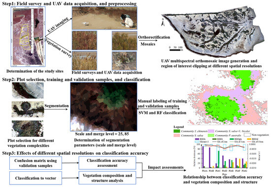
Figure 2.
The schematic process of the workflow of this study.
Based on the 2 cm spatial resolution UAV true color orthomosaic images and a priori knowledge from the field survey, the training and validation data for tidal marsh vegetation community classes were mainly selected from 2 cm spatial resolution UAV multispectral orthomosaic images (Table 1), and appropriate adjustments were made in the classification of 5 cm and 10 cm spatial resolution images to reduce the errors that may be brought about by data mismatches and differences in lighting conditions. The OEFESVM approach was implemented in ENVI 5.5 software (Harris Inc., Boulder, CO, USA), and the segmentation parameters were set to favor classification quality for every plot by repeated visual comparison, and applied for all five bands of imagery (Table 1).
The RF was performed based on images from all five bands using the ImageRF Classification embedded in the EnMAP-Box V2.2.0, which is a free and open toolbox developed at Humboldt-Universitaet zu Berlin, Geography Department, Geomatics Lab, under Deutsches GeoForschungsZentrum contract. The ntree (the number of trees to be grown, with the default value in ntree = 500) and mtry (the number of possible splitting variables to be considered at each tree node, with the default value of mtry = the number of the square root of the total predictive variables), the two main tuning parameters in RF, were set to their default values because these have proven to be a good choice [33,34].
The classification accuracy assessment was based on the confusion matrix, in which the OA, Kappa coefficient (kappa), UA, and PA were calculated [35]. An accuracy assessment was conducted using ENVI 5.5 software (Harris Inc., Boulder, CO, USA).
2.5. Analysis of Vegetation Composition and Structure
Vegetation composition and structure were analyzed based on the classification results with the highest overall accuracy for each plot. Based on the previous studies [36,37,38,39,40,41,42], variables commonly used to characterize vegetation composition and structure were selected as shown in Table 2, and were used to indicate the vegetation complexity of different plots.
Table 2.
Variables used to characterize vegetation composition and structure in this study.
2.6. Statistical Test
The multiple independent samples nonparametric Jonckheere–Terpstra test at a 5% level of significance was used to determine whether there was a significant difference in overall accuracy among three spatial resolution images, and there was a significant difference of vegetation complexity among the different plots. The Jonckheere–Terpstra test is suitable for detecting a significant difference among multiple groups of small sample sizes without requiring assumptions of normality and homogeneity of variance [43]. Statistical tests were implemented in the Statistical Package for Social Sciences (SPSS) version 19 for Windows (IBM Corp., Armonk, NY, USA).
3. Results
3.1. Quantitative Comparison of Classification Overall Accuracy
The classification accuracy of the vegetation community generated by the OEFESVM approach is shown in Table A1 in Appendix A. The classification accuracy based on the RF method is presented in Table A2 in Appendix A.
In general, the classification accuracy of the OEFESVM approach outperformed that of the RF method (Figure 3). The overall accuracy trends of the two classification methods across the seven plots were consistent, with PlotA exhibiting the highest classification accuracy and PlotD and PlotG showing the lowest. Due to paper length constraints, the results were primarily presented as the classification outcomes from the OEFESVM approach.
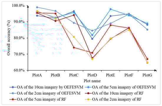
Figure 3.
Overall accuracy for seven plots generated by the object-oriented example-based feature extraction with support vector machine (OEFESVM) approach and random forest (RF) classifier.
No statistically significant differences (p < 0.05) were detected in the OA values of three spatial resolution images from the two classifications across the seven plots. However, differences in classification results still existed. The highest classification accuracy generated by the OEFESVM approach was achieved with the 2 cm spatial resolution image of PlotA, with an OA of 98.94%, while the lowest accuracy was achieved with the 10 cm spatial resolution image of PlotD, with an OA of 79.43%. PlotA and PlotB did not contain P. australis, and the classification results were highly consistent with the common perception that the higher the spatial resolution of the image, the higher the classification accuracy. PlotD of the five plots with P. australis had the same trend as PlotA and PlotB, but had the lowest OA (79.43% for the 10 cm, 81.76% for the 5 cm, and 84.48% for the 2 cm spatial resolution imagery) of all seven plots. The comparison of classification accuracy among three spatial resolution images in PlotC and PlotF had results opposite to those of PlotA, PlotB, and PlotD, showing that the higher the spatial resolution of imagery, the lower the classification accuracy. The 5 cm spatial resolution images produced higher accuracy when compared with the 2 cm and 10 cm spatial resolution images in PlotE and PlotG.
The percentages of plots with the OA values generated by the OEFESVM approach exceeding 90% for spatial resolutions of 2 cm, 5 cm, and 10 cm were 42.9% (3/7), 71.4% (5/7), and 71.4% (5/7), respectively (Table A1). The percentages of plots with the OA values generated by the RF method exceeding 90% for spatial resolutions of 2 cm, 5 cm, and 10 cm were 28.6% (2/7), 28.6% (2/7), and 42.9% (3/7), respectively (Table A2). Among the seven plots, the maximum OA value in the OEFESVM approach was achieved by the 2 cm spatial resolution classification in four cases, while the 5 cm and 10 cm spatial resolutions each yielded two instances (Figure 3). On the other hand, the RF classification results showed only one instance at 2 cm spatial resolution, four at 5 cm, and two at 10 cm (Figure 3). Among the five plots containing P. australis (PlotC, PlotD, PlotE, PlotF, and PlotG), only the maximum OA values from the OEFESVM classification result of PlotD came from a 2 cm spatial resolution image, while two plots each used 5 cm and 10 cm resolutions, respectively. In the RF classification results, three plots used 5 cm resolution and two plots used 10 cm resolution.
In terms of a mean OA across all seven plots, the 5 cm spatial resolution UAV image obtained slightly better classification results than the other two spatial resolution images from the OEFESVM approach. The 2 cm spatial resolution imagery produced high OA values for all plots, ranging from 84.48% to 98.94% with a 14.46% difference, and a mean accuracy 91.16%. The accuracy from the 5 cm spatial resolution imagery was between 81.76% and 97.74% with a 15.98% difference and a mean accuracy of 92.41%. The accuracy of the 10 cm spatial resolution imagery ranged between 79.43% and 96.49% with a 17.06% difference and a mean accuracy of 91.17%. In general, a random sample in the classification map had a higher probability of being correctly classified as P. australis or S. salsa + L. bicolor, and a lower probability of being correctly classified as S. salsa or T. chinensis.
Within seven plots, non-vegetation was classified by the OEFESVM approach with high accuracy (PA > 99.73% and UA > 97.83%) in all three spatial resolution images. The PA and UA values varied among vegetation communities (Table A1 and Table A2). From the PA value, we found that generally, the 2 cm spatial resolution images outperformed the 5 cm and 10 cm spatial resolution images in the classification of S. salsa and T. chinensis, the 10 cm spatial resolution images outperformed the other two spatial resolution images in the classification of the P. australis, and the 2 cm and 5 cm spatial resolution images were better suited for classifying S. salsa + L. bicolor (Table 3).
Table 3.
The maximum (Max.), minimum (Min.), mean, and difference of produced (PA) and user (UA) accuracy for the vegetation community classification of all plots.
In terms of mean PA values generated by the OEFESVM approach, omission classification of T. chinensis and S. salsa + L. bicolor was less likely to result from the 2 cm spatial resolution image, S. salsa from the 5 cm spatial resolution image, and P. australis from the 10 cm spatial resolution image, while in terms of mean UA values, fewer samples were misclassified as P. australis in the classification results of the 2 cm spatial resolution image, fewer samples were misclassified as S. salsa or T. chinensis in the classification results of the 5 cm spatial resolution image, and fewer samples were misclassified as S. salsa + L. bicolor in the classification results of the 10 cm spatial resolution image (Table 3).
3.2. Qualitative Comparison of Classification Accuracy
For the sake of conciseness, three out of the seven plots, i.e., PlotA, PlotD, and PlotF, in other words nine out of the twenty-one classifications, were selected to qualitatively evaluate the classification results from three different spatial resolutions of UAV imagery through visual interpretation (Figure 4, Figure 5 and Figure 6).
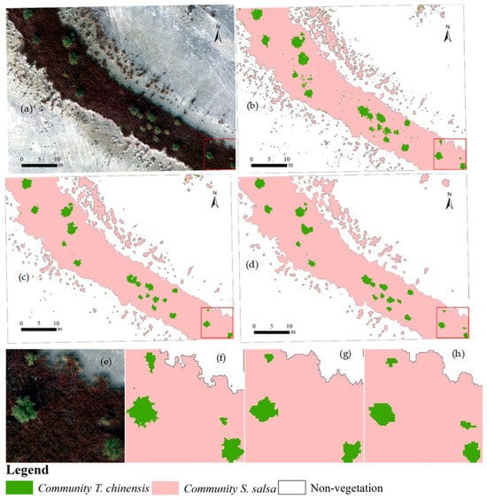
Figure 4.
Vegetation composition and structure of PlotA. The red frame in the lower right of (a–d) represented the region shown in (e–h). (a) The RGB image; (b) vegetation classification map of the 2 cm spatial resolution image; (c) vegetation classification map of the 5 cm spatial resolution image; (d) vegetation classification map of the 10 cm spatial resolution image; (e) subset of (a); (f) subset of (b); (g) subset of (c); and (h) subset of (d).
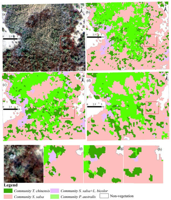
Figure 5.
Vegetation composition and structure of PlotD. The red frame in the middle-right of (a–d) represented the region shown in (e–h). (a) The RGB image; (b) vegetation classification from the 2 cm spatial resolution image; (c) vegetation classification from the 5 cm spatial resolution image; (d) vegetation classification from the 10 cm spatial resolution image; (e) subset of (a); (f) subset of (b); (g) subset of (c); and (h) subset of (d).
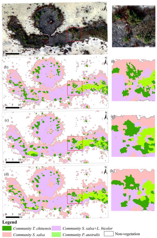
Figure 6.
Vegetation composition and structure of PlotF. The red frame in the center of (a–d) represented the region shown in (e–h). (a) The RGB image; (b) vegetation classification from the 2 cm spatial resolution image; (c) vegetation classification from the 5 cm spatial resolution image; (d) vegetation classification from the 10 cm spatial resolution image; (e) subset of (a); (f) subset of (b); (g) subset of (c); and (h) subset of (d).
In PlotA (Figure 4), as the spatial resolution increased from 10 cm to 5 cm to 2 cm, more vegetation patches were classified, more small-sized vegetation patches were detected, and the T. chinensis patches were detected with more complete morphology and more zigzagged edges (Figure 4f–h), and the 5 cm spatial resolution image did not detect the small T. chinensis patch in the lower right of the image (Figure 4c,g).
Compared with PlotA, the vegetation structure in PlotD was more complex (Figure 5a,e), the OA values of three spatial resolution images were low (Table A1 and Table A2), the patch sizes of P. australis and T. chinensis were overestimated to varying degrees, and many small vegetation patches were not detected (Figure 5b–d). The size of some T. chinensis patches were overestimated in the 10 cm and 5 cm spatial resolution images, and underestimated in the 2 cm spatial resolution images, and the area and number of P. australis patches were overestimated in the 5 cm and 10 cm spatial resolution images (Figure 5f–h).
In PlotF, the 2 cm and 5 cm spatial resolution images overestimated the number and area of T. chinensis patches, and the 10 cm spatial resolution image overestimated the area of some T. chinensis patches (Figure 6). The 2 cm spatial resolution image underestimated the number and area of P. australis patches (Figure 6b,f), the 5 cm spatial resolution image overestimated the number and size of P. australis patches (Figure 6c,g), and visually, the classification result from the 10 cm spatial resolution image was better (Figure 6d,h).
We compared five plots containing P. australis (PlotC, PlotD, PlotE, PlotF, and PlotG) and found that the greener the P. australis, the more it coexisted with T. chinensis, and the lower the overall accuracy.
3.3. Vegetation Structure of the Seven Plots
A significant difference (p < 0.05) was only observed in terms of the number of P. australis (p = 0.033), vegetation cover of community S. salsa + L. bicolor (p = 0.015), area of community S. salsa + L. bicolor (p = 0.015), and the relative dominance of community S. salsa + L. bicolor (p = 0.033) among the seven plots. However, differences in vegetation composition and structure among seven plots still existed. PlotD, of all seven plots, had the highest vegetation cover (90.2%), vegetation cover of S. salsa patches (47.6%) and vegetation cover of T. chinensis patches (11.1%), followed by PlotG with 63.8% vegetation cover and 8.4% vegetation cover of T. chinensis patches, and PlotC with 62.7% vegetation cover and the highest vegetation cover of P. australis patches (45.6%). PlotF had the highest vegetation cover of S. salsa + L. bicolor patches (19.2%), and PlotA had 34.1% with the lowest vegetation cover (Figure 7a).
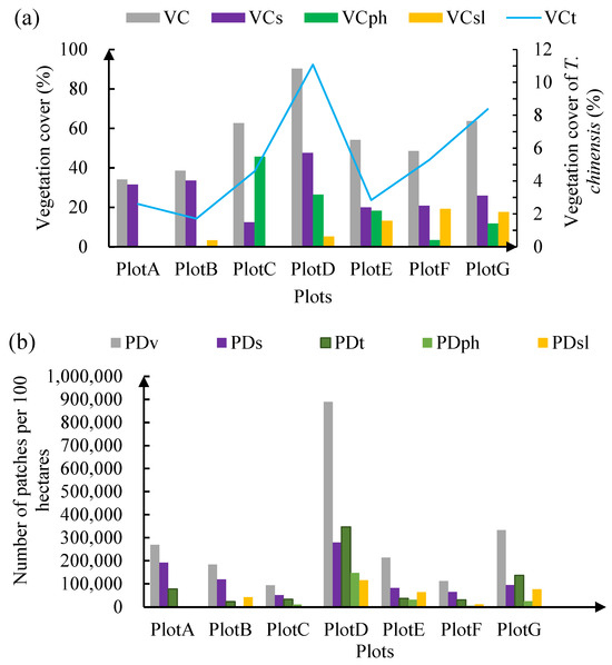
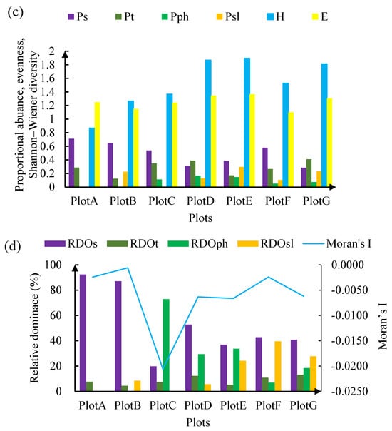
Figure 7.
Vegetation composition and structure of seven plots. (a) Vegetation cover (VC), vegetation cover of S. salsa patches (VCs), T. chinensis patches (VCt), P. australis patches (VCph), and S. salsa + L. bicolor patches (VCsl); (b) number of vegetation patches per 100 hectares (PDv), number of S. salsa patches per 100 hectares (PDs), number of T. chinensis patches per 100 hectares (PDt), number of P. australis patches per 100 hectares (PDph), and number of S. salsa + L. bicolor patches per 100 hectares (PDsl); (c) proportional abundance of S. salsa patches (Ps), T. chinensis patches (Pt), P. australis patches (Pph), and S. salsa + L. bicolor patches (Psl), and Shannon–Wiener diversity (H), and evenness (E); and (d) relative dominance of S. salsa patches (RDOs), T. chinensis patches (RDOt), P. australis patches (RDOph), S. salsa + L. bicolor patches (RDOsl), and Moran’s I.
PlotD, of all seven plots, had the highest number of vegetation patches, S. salsa, T. chinensis, P. australis, and S. salsa + L. bicolor patches per 100 hectares, followed by PlotG and PlotA (Figure 7b).
PlotD had four kinds of vegetation communities: S. salsa, T. chinensis, S. salsa + L. bicolor, and P. australis; the relative dominance of S. salsa was 52.7%, which was 4.3 times that of T. chinensis, 9.3 times that of S. salsa + L. bicolor, and 1.8 times that of P. australis; the vegetation pattern was complex with a low Moran’s I value, high Shannon–Wiener diversity index, and high evenness value (Figure 7), and P. australis showed withered yellow or green color, which made it easy to confuse with green T. chinensis. Moreover, it often grew mixed with T. chinensis (Figure 5a), and the OA values of the three kinds of spatial resolution images were the lowest across all seven plots, with the lowest OA of 79.4% (Table A1).
PlotA had the highest proportional abundance of S. salsa patches (0.71), PlotG had the highest proportional abundance of T. chinensis patches (0.41), PlotD had the highest proportional abundance of P. australis patches (0.17), and PlotE had 0.30 with the highest proportional abundance of S. salsa + L. bicolor patches (Figure 7c).
The Shannon–Wiener diversity index (Figure 7c) showed that PlotD and PlotE had the highest Shannon–Wiener diversity, followed by PlotG, and the species evenness was high for PlotD, PlotE, and PlotG (Figure 7c).
The relative dominance of S. salsa patches was the highest in the other six plots, except for PlotC, which had the highest relative dominance of P. australis patches (Figure 7d).
The Moran’s I values of all seven plots were less than 0.0, with PlotC having the smallest value (−0.0206), followed by PlotE (−0.0066), PlotD (−0.0063) and PlotG (−0.0062), indicating a random distribution of vegetation patches in the plots (Figure 7d).
Among all seven plots, PlotC had the smallest Moran’s I value, indicating the greatest spatial variation; the relative dominance of P. australis was 72.8%, the proportional abundance of T. chinensis was 0.35 (Figure 7), P. australis and T. chinensis were similar in color, and the images with higher spatial resolution (2 cm) segmented more P. australis and T. chinensis patches, resulting in higher mixing and lower classification accuracy (Table A1). The OA values generated by the OEFESVM of all three spatial resolution images of PlotF exceeded 93.9%, and the difference between them was less than 1%, the OA value of the 10 cm spatial resolution image was only 0.19% higher than that of the 2 cm spatial resolution image, and its value of Moran’s I was close to 0.0, indicating minimal spatial differences, relatively high Shannon–Wiener diversity index and proportional abundance of T. chinensis, and the largest value of relative dominance of S. salsa + L. bicolor, followed by the relative dominance value of S. salsa. The mixing between S. salsa + L. bicolor and S. salsa was responsible for the slightly lower precision of the finer spatial resolution images. PlotE and PlotG had small values of Moran’s I, high spatial variation, high Shannon–Wiener diversity index and evenness index, relatively fragmented vegetation patches, high proportional abundance of S. salsa + L. bicolor, low proportional abundance of S. salsa, and relatively coarser spatial resolution images to obtain high classification accuracy. Compared with PlotE, the OA value of PlotG was substantially lower, probably related to the high proportional abundance of T. chinensis (0.41) in PlotG. Similarly, PlotD, which had high proportional abundance of T. chinensis (0.39) and the highest proportional abundance of P. australis, had the lowest OA values.
4. Discussion
Vegetation is an important component of tidal marsh ecosystems, and fine-scale mapping of its composition and structure is essential for the development of conservation and restoration strategies for tidal marsh ecosystems [14]. The use of UAV imagery for vegetation mapping has become one of the most important means [44]. It is obvious that the spatial resolution should be smaller than the size of vegetation patches [45], and different spatial resolutions should be chosen for scenes with different vegetation composition and structure. However, there is still a trade-off between imaging spatial resolution and imaging extent in the current UAV image acquisition [22,23], and the effectiveness of different spatial resolutions must be evaluated before vegetation mapping, so as to achieve high cost-effectiveness with the appropriate spatial resolution. This study tried to answer this question by selecting seven plots with different vegetation complexities in the YRD of China and using UAV images with three different spatial resolutions: 10 cm, 5 cm, and 2 cm.
4.1. Vegetation Characteristics and Classification Accuracy
Tidal marshes were characterized by strong spatial heterogeneity and high vegetation diversity due to topographic and water-salinity variations [14]. Accurately mapping the vegetation composition and structure of tidal marshes using remote sensing technology is challenging since the vegetation characteristics of tidal marshes are highly variable spatially and similar in spectral characteristics. The accuracy of vegetation mapping was strongly related to the spectral, spatial, and temporal resolution of the remote sensing data used [46]. This study focused only on the effect of image spatial resolution on vegetation classification accuracy.
UAV imagery has become one of the most important types of data for mapping vegetation [44]; however, there are few systematic analyses for deciding what kind of spatial resolutions are needed in mapping vegetation characteristics in spatially heterogeneous regions [10,19]. Inadequate coarse spatial resolution images can reduce the accuracy of vegetation classification [21]. Improving the spatial resolution of images requires more labor and time [21,22,24]. Imaging the same region with spatial resolutions ranging from 10 cm, to 5 cm, to 2 cm would significantly increase the flight time of the UAV, the number of battery packs consumed and images taken, and data volume (Table 4). For users with limited time and budgets, such as fellow researchers and ecological monitors in nature reserves, it is essential to know the appropriate spatial resolution for the UAV imagery for fine-scale mapping of vegetation communities.
Table 4.
Summary of flight parameters for imaging a 1 km2 area at 10 cm, 5 cm, and 2 cm spatial resolution using a DJI Phantom 4 Multispectral unmanned aerial vehicle.
Vegetation classification accuracy increases as the spatial resolution of the image is increased [19,47,48]. This is consistent with the classification results of PlotA, PlotB, and PlotD in that their OA values gradually increased with increasing the spatial resolution from 10 cm to 2 cm. Analyzing the vegetation composition and structure indexes (Figure 7), this may be related to the high relative dominance of S. salsa in the three plots, which exceeded 52% (Figure 7d). PlotA had only two kinds of vegetation, S. salsa and T. chinensis, and the relative dominance of S. salsa reached 92.4%, which was 12 times higher than that of T. chinensis, showing the spatial pattern of T. chinensis sporadically embedded in S. salsa. The vegetation pattern was relatively simple (Figure 4), the two kinds of vegetation had obvious differences in both colors and plant heights in this season, and the OAs of all three spatial resolution images were more than 93% (Table A1). PlotB had three kinds of vegetation: S. salsa, T. chinensis, and S. salsa + L. bicolor. The relative dominance of S. salsa reached 87.1%, which is 19.6 times higher than that of T. chinensis, and 10.2 times higher than that of S. salsa + L. bicolor, presenting the spatial pattern of a small amount of T. chinensis scattered in S. salsa, and a sporadic distribution of S. salsa + L. bicolor in S. salsa close to the interior of vegetation patches. The vegetation pattern was relatively simple, the three kinds of vegetation colors were obviously different (purple S. salsa, green T. chinensis, and gray or white S. salsa + L. bicolor), and the OA values of all three spatial resolution images exceeded 92% (Table A1). These findings suggested that for relatively low vegetation complexity in the plots with low spectral similarity between vegetation communities, even images with relatively low spatial resolution can achieve high classification accuracy, and this is consistent with previous studies [19,21,49].
There have been contrasting opinions about vegetation classification accuracy increases as the spatial resolution of the image is increased. Some have debated that improving spatial resolution can make classification difficult [21]. Some have indicated that the classification accuracy of a homogeneous class is not affected by the spatial resolution [50]. Some have showed that the classification accuracy of the quasi-circular vegetation patches could not be improved with increasing spatial resolution from 5 m to 1 m [32]. Our results showed that the highest classification accuracies generated by the OEFESVM and RF approaches were obtained by using 10 cm spatial resolution images in PlotC and PlotF, and by using the 5 cm spatial resolution images in PlotE and PlotG (Table A1). This may be due to vegetation complexity affecting the classification accuracy [49,51]. As spatial resolution increases, the similarity in color between green P. australis and T. chinensis during the study period, coupled with the frequent co-occurrence of the two species, resulted in some training and validation samples of P. australis exhibiting characteristics more akin to T. chinensis. This reduced classification accuracy.
From the perspective of vegetation classification, three of the seven plots had the highest classification accuracy from the 2 cm spatial resolution images using the OEFESVM approach (Table A1). In particular, for PlotA with only two vegetation types, S. salsa and T. chinensis, and PlotB with three vegetation types, S. salsa, T. chinensis, and S. salsa + L. bicolor, their vegetation complexities were relatively low, and the proportional abundance and relative dominance of S. salsa was very large, which made the classification of the 2 cm spatial resolution images more advantageous. However, we argued that the 2 cm spatial resolution images were not necessarily used for mapping vegetation in whole landscapes, because almost as high classification accuracy was derived when using the 5 cm spatial resolution images for classifying vegetation. Our results showed that for the plots with high vegetation complexity, P. australis and T. chinensis with high proportional abundance, the highest classification accuracies generated by the OEFESVM and RF approaches were obtained with the 5 cm or 10 cm spatial resolution images. This finding was not consistent with former conclusions [21], which needs to be further studied in the future. This may be attributed to the fact that coarse spatial resolution images classified the pixels containing both P. australis and T. chinensis as P. australis, yielding results closer to conventional vegetation classification.
4.2. Statistical Metrics of Vegetation Complexity
Vegetation complexity affected the vegetation classification map obtained from the remotely sensed images [49,51]. Some have used multiple landscape pattern indices to analyze the classification uncertainties of various urban green space landscapes [49]. This study used the proportional abundance, relative dominance, Shannon’s index, evenness index, and Moran’s index to analyze the relationships between classification accuracy and image spatial resolutions. The entropy-based index and Gray-based index have been used to detect the complexity of geo-surface scenes from remotely sensed data [42]. This study suggested that landscape complexity metrics that cooperatively consider the vegetation spatial pattern and the spectral similarity of vegetation communities need to be developed to better determine landscape complexity and to analyze the relationship between classification accuracy and image spatial resolution.
4.3. Prospects
Accurate classification of vegetation requires consideration of the spectral, spatial, and temporal resolution of remotely sensed images and the classification approaches used, and vegetation phenology and height data can help improve classification accuracy [8,21,46,52]. This study analyzed what kind of spatial resolution for UAV images was needed for mapping vegetation in a tidal marsh; some aspects need to be studied in depth.
This study applied the object-oriented example-based feature extraction with support vector machine approach and random forest classifier to map vegetation and evaluate the differences in classification accuracy under three spatial resolutions. In general, the overall accuracy trends of the two classification methods across the seven plots were consistent, and the classification accuracy of the OEFESVM approach outperformed that of the RF method. Compared to the pixel-based RF method, improving image spatial resolution could yield greater gains in classification accuracy for the object-oriented example-based feature extraction with support vector machine approach. Multiple advanced approaches (for example, deep learning algorithms) should be employed to assess variations in vegetation mapping in a tidal marsh at different spatial resolutions in the future [16,29,53]. In addition, the effects of different segmentation scales of the object-oriented approaches on the classification accuracy of the different spatial resolutions should also be considered [16,19]. The selection of training and validation samples for vegetation communities in centimeter-level spatial resolution imagery, particularly in mixed vegetation zones, significantly influences classification accuracy, and warrants further investigation.
In this study, the effect of different spatial resolutions on classification accuracy was only evaluated using UAV data acquired in late fall when the vegetation color difference was large, and it remains to be demonstrated whether the conclusions of this study are applicable to the comparison of classification accuracy of images acquired in other seasons, as the vegetation spectral and color characteristics vary seasonally. For single-season images, high classification accuracy will be facilitated by utilizing images acquired during the seasons when the differences between various vegetation types are most pronounced, and specifically for the study area, mid- to late-fall is one of the best times of year for vegetation classification. In general, time-series imagery can improve classification accuracy compared to single-season imagery. The effect of different spatial resolution time-series images on vegetation classification accuracy may be a direction that can be studied in the future. In addition to vegetation phenology, hyperspectral features and vegetation canopy height information have the potential to be utilized to improve classification accuracy and also need to be considered in the future [14,54].
Although seven plots were explored, the relatively small plots and the limited number of plots may influence the generalizability of the results of this study to larger or other tidal marsh ecosystems. However, it is certain that vegetation classification for tidal marshes with different complexities of vegetation composition and structure should utilize images with different spatial resolutions acquired at appropriate dates in order to obtain cost-effective vegetation classification maps.
In the short term, UAV technology will continue to face the trade-off between spatial resolution and imaging extent [22,23]. For the time being, the centimeter-level spatial resolution UAV data acquired in localized areas to assist in field vegetation surveys for the generation of training and validation data, as well as the acquisition of meter-level spatial resolution satellite data over large coverage areas for vegetation mapping may be possible ways to achieve fine mapping of vegetation over large areas. Some studies have explored the applicability of integrated UAV and satellite images; spectral, spatial, and temporal fusions still need to be studied [10,46].
Although no statistically significant differences (p < 0.05) were detected in the OA values of three spatial resolution images from the two classifications across the seven plots, considering the proportion of maximum classification overall accuracy across seven plots for three spatial resolutions, particularly in the five plots containing P. australis, and taking into account data processing time and costs of the UAV, this study suggested that a 5 cm spatial resolution imagery should be used for mapping vegetation in tidal marshes in the YRD, China, or other regions with similar vegetation composition and structure. For classifying salt marsh vegetation in other regions, it is recommended to capture drone imagery during periods with significant phenological differences among vegetation communities. Selecting drone imagery with appropriate spatial resolution ensures classification accuracy, whereas using images with excessively high spatial resolution may actually reduce classification accuracy in areas with severe vegetation mixing. Although the different spatial resolution images should be chosen for scenes with different vegetation complexities, this would take more manpower, time, and resources. This issue can be addressed by the future development of UAVs equipped with automatic configuration functions for optimal flight parameters tailored to the different vegetation complexities of different regions.
In practical applications, it is recommended to utilize existing meter- or sub-meter-level images and field survey data for preliminary classification, calculate classification accuracy indexes and vegetation complexity indexes, and for areas with low classification accuracy and high vegetation complexity, improve the imaging spatial resolution or temporal resolution to obtain vegetation maps with higher classification accuracy. In addition, taking into account the risk of loss or destruction of UAVs due to falling or sinking into tidal marshes, the UAV data should be acquired based on the complexity of vegetation composition, structure, and spatial pattern, combined with high spatial resolution and time-series satellite imagery to regularize vegetation monitoring in the study area.
5. Conclusions
This study compared three fine spatial resolution UAV multispectral orthomosaics to map vegetation in tidal marshes in the YRD, China, and evaluated the effects of spatial resolution on classification accuracy. The main results showed the following: (1) The vegetation classification map varied at different spatial resolutions. The difference between the most and least accurate classification accuracy was 0.95–8.76 percentage points on three different spatial resolution images in the different plots. (2) Vegetation complexity impacted vegetation classification accuracy. When the number of vegetation communities was small and the spatial pattern of vegetation was simple, the classification accuracy increased with increasing spatial resolution. On the contrary, when the number of vegetation communities was large and the spatial pattern of vegetation was complex, the relatively coarser spatial resolution images could obtain higher classification accuracy. In general, classification accuracy was lower when the relative dominance and proportional abundance of P. australis and T. chinensis were high in the plots. (3) Considering the trade-off between classification accuracy and imaging extent, a 5 cm spatial resolution UAV imagery was recommended for tidal marsh vegetation classification in the YRD or other regions with similar vegetation composition and structure.
Future research can explore more advanced approaches to assess the impacts of spatial resolution on mapping vegetation in tidal marshes and seek more appropriate statistical metrics of vegetation pattern complexity to better address the relationships between vegetation composition and spatial pattern and classification accuracy at different spatial resolutions. Although focused only on spatial resolution, this study suggested that the effect of different spatial resolutions on classification accuracy should be investigated in the future under different phenological periods of vegetation communities.
Author Contributions
Conceptualization, Q.L., X.Z., and Z.L.; methodology, Q.L., C.H., X.Z., H.L., and S.W.; validation, Q.L., H.L., Y.P., and L.G.; investigation, Q.L., S.W., Y.P., and L.G.; data curation, Q.L.; writing—original draft preparation, Q.L. and S.W.; writing—review and editing, Q.L., C.H., H.L., X.Z., S.W., Y.P., L.G., and Z.L.; funding acquisition, Q.L. and X.Z. All authors have read and agreed to the published version of the manuscript.
Funding
This research was funded by the National Key Research and Development Program of China, grant number 2021YFB3901305; the QILU RESEARCH INSTITUTE, grant number QLZB76-2023-000059; and the Open Foundation of the Key Laboratory of Natural Resource Coupling Process and Effects, grant number 2023KFKTB003. The APC was funded by the QILU RESEARCH INSTITUTE, grant number QLZB76-2023-000059, and the Open Foundation of the Key Laboratory of Natural Resource Coupling Process and Effects, grant number 2023KFKTB003.
Data Availability Statement
Data are unavailable due to privacy or ethical restrictions.
Conflicts of Interest
The authors declare no conflicts of interest.
Appendix A. The Vegetation Community Classification Accuracy for Seven Plots in the Study Area
Table A1.
Vegetation community classification accuracy for seven plots generated by the OEFESVM approach.
Table A1.
Vegetation community classification accuracy for seven plots generated by the OEFESVM approach.
| Plot Name | Spatial Resolution | OA | Kappa | S. salsa | T. chinensis | P. australis | S. salsa + L. bicolor | Non-Vegetation | |
|---|---|---|---|---|---|---|---|---|---|
| (cm) | (%) | (%) | (%) | (%) | (%) | (%) | |||
| PlotA | 10 | 93.75 | 0.8972 | PA | 99.96 | 66.76 | 100.0 | ||
| UA | 83.19 | 100.0 | 99.97 | ||||||
| 5 | 96.23 | 0.9378 | PA | 99.88 | 79.47 | 100.0 | |||
| UA | 89.03 | 100.0 | 99.93 | ||||||
| 2 | 98.94 | 0.9824 | PA | 100.0 | 93.97 | 100.0 | |||
| UA | 96.64 | 100.0 | 100.0 | ||||||
| PlotB | 10 | 92.01 | 0.8731 | PA | 98.18 | 66.41 | 76.41 | 99.90 | |
| UA | 78.09 | 99.12 | 89.67 | 97.83 | |||||
| 5 | 92.54 | 0.8796 | PA | 80.27 | 82.09 | 90.57 | 99.98 | ||
| UA | 85.81 | 99.50 | 69.65 | 98.92 | |||||
| 2 | 96.63 | 0.9440 | PA | 99.65 | 82.07 | 89.88 | 100.0 | ||
| UA | 86.35 | 99.93 | 98.90 | 99.78 | |||||
| PlotC | 10 | 96.49 | 0.9240 | PA | 72.54 | 74.57 | 97.68 | 99.97 | |
| UA | 80.31 | 67.64 | 97.84 | 99.30 | |||||
| 5 | 95.73 | 0.9087 | PA | 89.16 | 93.00 | 94.76 | 99.96 | ||
| UA | 51.53 | 72.53 | 99.31 | 99.86 | |||||
| 2 | 89.32 | 0.7920 | PA | 98.49 | 99.27 | 84.96 | 99.96 | ||
| UA | 26.93 | 41.00 | 99.97 | 100.0 | |||||
| PlotD | 10 | 79.43 | 0.6876 | PA | 96.55 | 76.01 | 76.37 | 42.58 | 99.88 |
| UA | 46.70 | 72.64 | 97.67 | 73.05 | 99.88 | ||||
| 5 | 81.76 | 0.7152 | PA | 98.91 | 90.27 | 74.37 | 79.39 | 100.0 | |
| UA | 54.08 | 49.27 | 99.21 | 77.49 | 99.61 | ||||
| 2 | 84.48 | 0.7528 | PA | 97.73 | 92.71 | 77.60 | 91.87 | 99.73 | |
| UA | 56.62 | 50.71 | 99.29 | 90.78 | 99.93 | ||||
| PlotE | 10 | 93.49 | 0.9104 | PA | 95.54 | 94.83 | 88.05 | 95.74 | 99.81 |
| UA | 88.89 | 42.38 | 98.22 | 98.07 | 99.30 | ||||
| 5 | 97.74 | 0.9681 | PA | 98.82 | 91.14 | 96.77 | 96.84 | 99.96 | |
| UA | 98.75 | 62.62 | 99.00 | 98.80 | 99.71 | ||||
| 2 | 88.98 | 0.8459 | PA | 57.24 | 98.84 | 90.53 | 97.11 | 99.84 | |
| UA | 73.04 | 60.94 | 99.89 | 67.19 | 99.99 | ||||
| PlotF | 10 | 94.85 | 0.9253 | PA | 90.55 | 91.59 | 83.81 | 94.49 | 99.19 |
| UA | 78.40 | 92.70 | 99.73 | 94.27 | 98.59 | ||||
| 5 | 93.90 | 0.9114 | PA | 93.94 | 95.87 | 62.02 | 98.99 | 100.0 | |
| UA | 86.05 | 76.46 | 99.88 | 91.96 | 99.40 | ||||
| 2 | 94.66 | 0.9214 | PA | 98.95 | 98.57 | 64.81 | 97.23 | 100.00 | |
| UA | 77.89 | 85.45 | 99.78 | 92.96 | 99.94 | ||||
| PlotG | 10 | 88.16 | 0.8315 | PA | 76.86 | 76.93 | 86.02 | 91.84 | 100.0 |
| UA | 55.18 | 59.24 | 97.83 | 88.63 | 98.73 | ||||
| 5 | 88.94 | 0.8408 | PA | 88.10 | 75.16 | 85.72 | 94.17 | 100.0 | |
| UA | 47.57 | 74.73 | 98.19 | 83.28 | 99.77 | ||||
| 2 | 85.15 | 0.7896 | PA | 92.14 | 87.57 | 75.19 | 98.29 | 99.99 | |
| UA | 51.91 | 55.94 | 99.67 | 73.91 | 99.93 |
OA—overall accuracy, Kappa—Kappa coefficient, PA—producer’s accuracy, and UA—user’s accuracy. The bolded data were those with the highest overall accuracy for each plot.
Table A2.
Vegetation community classification accuracy for seven plots generated by the random forest method.
Table A2.
Vegetation community classification accuracy for seven plots generated by the random forest method.
| Plot Name | Spatial Resolution | OA | Kappa | S. salsa | T. chinensis | P. australis | S. salsa + L. bicolor | Non-Vegetation | |
|---|---|---|---|---|---|---|---|---|---|
| (cm) | (%) | (%) | (%) | (%) | (%) | (%) | |||
| PlotA | 10 | 95.45 | 0.9254 | PA | 99.80 | 76.09 | 100.0 | ||
| UA | 87.35 | 99.82 | 99.87 | ||||||
| 5 | 95.45 | 0.8248 | PA | 99.93 | 75.10 | 100.0 | |||
| UA | 87.05 | 100.0 | 99.92 | ||||||
| 2 | 96.67 | 0.945 | PA | 96.41 | 87.36 | 99.99 | |||
| UA | 92.98 | 93.37 | 99.98 | ||||||
| PlotB | 10 | 90.46 | 0.8488 | PA | 97.95 | 59.20 | 72.92 | 99.81 | |
| UA | 77.82 | 97.23 | 77.26 | 97.99 | |||||
| 5 | 95.05 | 0.9197 | PA | 98.54 | 79.10 | 86.07 | 99.38 | ||
| UA | 86.65 | 98.04 | 89.99 | 98.83 | |||||
| 2 | 91.98 | 0.8659 | PA | 99.45 | 71.08 | 57.10 | 100.0 | ||
| UA | 74.25 | 94.33 | 91.56 | 99.86 | |||||
| PlotC | 10 | 94.12 | 0.8753 | PA | 62.32 | 76.71 | 94.78 | 99.82 | |
| UA | 44.08 | 76.71 | 97.14 | 99.53 | |||||
| 5 | 74.11 | 0.5779 | PA | 85.36 | 86.54 | 64.25 | 99.92 | ||
| UA | 12.85 | 28.55 | 98.29 | 99.71 | |||||
| 2 | 80.63 | 0.6398 | PA | 42.71 | 69.31 | 98.13 | 76.44 | ||
| UA | 8.76 | 29.38 | 95.42 | 96.00 | |||||
| PlotD | 10 | 67.55 | 0.5767 | PA | 87.55 | 78.83 | 49.98 | 46.07 | 100.0 |
| UA | 56.41 | 36.10 | 82.22 | 79.76 | 99.30 | ||||
| 5 | 70.88 | 0.6162 | PA | 93.51 | 83.00 | 52.68 | 62.69 | 100.0 | |
| UA | 60.92 | 32.82 | 92.47 | 61.78 | 98.60 | ||||
| 2 | 66.94 | 0.5697 | PA | 97.26 | 69.51 | 44.53 | 58.63 | 99.82 | |
| UA | 50.06 | 41.04 | 92.74 | 56.89 | 93.20 | ||||
| PlotE | 10 | 79.50 | 0.7316 | PA | 92.52 | 90.92 | 58.22 | 90.25 | 99.61 |
| UA | 58.33 | 24.00 | 93.77 | 94.01 | 99.67 | ||||
| 5 | 87.86 | 0.8318 | PA | 85.34 | 77.90 | 82.80 | 86.75 | 99.85 | |
| UA | 72.34 | 40.13 | 92.63 | 91.00 | 99.36 | ||||
| 2 | 79.79 | 0.7234 | PA | 79.27 | 80.84 | 70.95 | 72.50 | 99.50 | |
| UA | 48.28 | 36.74 | 89.75 | 92.28 | 99.87 | ||||
| PlotF | 10 | 86.24 | 0.8004 | PA | 87.71 | 90.34 | 10.89 | 93.86 | 100.00 |
| UA | 53.20 | 67.71 | 88.64 | 96.81 | 98.60 | ||||
| 5 | 86.11 | 0.7992 | PA | 91.69 | 93.07 | 12.24 | 96.21 | 99.42 | |
| UA | 49.78 | 73.44 | 81.36 | 93.40 | 99.06 | ||||
| 2 | 84.96 | 0.7801 | PA | 79.80 | 88.65 | 25.42 | 87.48 | 99.71 | |
| UA | 42.11 | 74.77 | 72.31 | 90.64 | 99.85 | ||||
| PlotG | 10 | 64.73 | 0.5648 | PA | 79.87 | 70.16 | 34.91 | 88.76 | 100.0 |
| UA | 31.00 | 27.96 | 95.06 | 84.21 | 98.41 | ||||
| 5 | 67.01 | 0.5887 | PA | 88.45 | 68.30 | 39.22 | 88.23 | 99.98 | |
| UA | 27.00 | 32.69 | 91.69 | 84.23 | 99.82 | ||||
| 2 | 64.85 | 0.5664 | PA | 84.27 | 70.91 | 28.03 | 90.88 | 97.91 | |
| UA | 25.35 | 39.07 | 85.47 | 70.94 | 99.80 |
OA—overall accuracy, Kappa—Kappa coefficient, PA—producer’s accuracy, and UA—user’s accuracy. The bolded data were those with the highest overall accuracy for each plot.
References
- Li, H.; Yang, S.L. Trapping effect of tidal marsh vegetation on suspended sediment, Yangtze Delta. J. Coast. Res. 2009, 25, 915–924. [Google Scholar] [CrossRef]
- Van Belzen, J.; Van de Koppel, J.; Kirwan, M.L.; Van der Wal, D.; Herman, P.M.J.; Dakos, V.; Kefi, S.; Scheffer, M.; Guntenspergen, G.R.; Bouma, T.J. Vegetation recovery in tidal marshes reveals critical slowing down under increased inundation. Nat. Commun. 2017, 8, 15811. [Google Scholar] [CrossRef]
- Correll, M.D.; Hantson, W.; Hodgman, T.P.; Cline, B.B.; Elphik, C.S.; Shrive, W.G.; Tymkiw, E.L.; Olsen, B.J. Fine-scale mapping of coastal plant communities in the northeastern USA. Wetlands 2019, 39, 17–28. [Google Scholar] [CrossRef]
- Gedan, K.B.; Kirwan, M.L.; Wolanski, E.; Barbier, E.B.; Silliman, B.R. The present and future role of coastal wetland vegetation in protecting shorelines: Answering recent challenges to the paradigm. Clim. Change 2011, 106, 7–29. [Google Scholar] [CrossRef]
- Duarte, C.M.; Losada, I.J.; Hendriks, I.E.; Mazarrasa, I.; Marba, N. The role of coastal plant communities for climate change mitigation and adaption. Nat. Clim. Change 2013, 3, 961–969. [Google Scholar] [CrossRef]
- Kearney, W.S.; Fagherazzi, S. Salt marsh vegetation promotes efficient tidal channel networks. Nat. Commun. 2016, 7, 12287. [Google Scholar] [CrossRef] [PubMed]
- Van Zelst, V.T.M.; Dijkstra, J.T.; Van Wesenbeeck, B.K.; Eilander, D.; Morris, E.P.; Winsemius, H.C.; Ward, P.J.; De Vries, M.B. Cutting the costs of coastal protection by integrating vegetation in flood defences. Nat. Cummun. 2021, 12, 6533. [Google Scholar] [CrossRef] [PubMed]
- Villoslada, M.; Bergamo, T.F.; Ward, R.D.; Burnside, N.G.; Joyce, C.B.; Bunce, R.G.H. Fine scale plant community assessment in coastal meadows using UAV based multispectral data. Ecol. Indic. 2020, 111, 105979. [Google Scholar] [CrossRef]
- Worthington, T.A.; Spalding, M.; Landis, E.; Maxwell, T.L.; Navarro, A.; Smart, L.S.; Murray, N.J. The distribution of global tidal marshes from Earth observation data. Glob. Ecol. Biogeogr. 2024, 33, e13852. [Google Scholar] [CrossRef]
- Chen, Z.Z.; Chen, J.J.; Yue, Y.M.; Lan, Y.P.; Ling, M.; Li, X.H.; You, H.T.; Han, X.W.; Zhou, G.Q. Tradeoffs among multi-source remote sensing images, spatial resolution, and accuracy for the classification of wetland plant species and surface objects based on the MRS_DeepLabV3+ model. Ecol. Inform. 2024, 81, 102594. [Google Scholar] [CrossRef]
- Higinbotham, C.B.; Alber, M.; Chalmers, A.G. Analysis of tidal marsh vegetation patterns in two Georgia estuaries using aerial photography and GIS. Estuaries 2004, 27, 670–683. [Google Scholar] [CrossRef]
- Rajakumari, S.; Mahesh, R.; Sarunjith, K.J.; Ramesh, R. Building spectral catalogue for salt marsh vegetation, hyperspectral and multispectral remote sensing. Reg. Stud. Mar. Sci. 2022, 53, 102435. [Google Scholar] [CrossRef]
- Wu, Z.; Zhao, S.; Zhang, X.; Sun, P.; Wang, L. Studies on interrelation between salt vegetation and soil salinity in the Yellow River Delta. Chin. J. Plant Ecol. 1994, 18, 184–193, (In Chinese with English abstract). [Google Scholar]
- Li, H.; Liu, Q.S.; Huang, C.; Zhang, X.; Wang, S.X.; Wu, W.; Shi, L. Variation in vegetation composition and structure across mudflat areas in the Yellow River Delta, China. Remote Sens. 2024, 16, 3495. [Google Scholar] [CrossRef]
- Dronova, I.; Kislik, C.; Dinh, Z.; Kelly, M. A review of unoccupied aerial vehicle use in wetland applications: Emerging opportunities in approach, technology, and data. Drones 2021, 5, 45. [Google Scholar] [CrossRef]
- Huang, Y.F.; Lu, C.Y.; Jia, M.M.; Wang, Z.L.; Su, Y.; Su, Y.L. Plant species classification of coastal wetlands based on UAV images and object-oriented deep learning. Biodivers. Sci. 2023, 31, 22411, (In Chinese with English abstract). [Google Scholar] [CrossRef]
- Fassnacht, E.E.; Latifi, H.; Sterenczak, K.; Modzelewska, A.; Lefsky, M.; Waser, L.T.; Straub, C.; Ghosh, A. Review of studies on tree species classification from remotely sensed data. Remote Sens. Environ. 2016, 186, 64–87. [Google Scholar] [CrossRef]
- Belluco, E.; Camuffo, M.; Ferrari, S.; Modenese, L.; Silvestri, S.; Marani, A.; Marani, M. Mapping salt-marsh vegetation by multispectral and hyperspectral remote sensing. Remote Sens. Environ. 2006, 105, 54–67. [Google Scholar] [CrossRef]
- Rasanen, A.; Virtanen, T. Data and resolution requirements in mapping vegetation in spatially heterogeneous landscapes. Remote Sens. Environ. 2019, 230, 111207. [Google Scholar] [CrossRef]
- Kolarik, N.E.; Gaughan, A.E.; Stevens, F.R.; Pricope, N.G.; Woodward, K.; Cassidy, L.; Salerno, J.; Hartter, J. A multi-plot assessment of vegetation structure using a micro-unmanned aerial system (UAS) in a semi-arid savanna environment. ISPRS J. Photogramm. Remote Sens. 2020, 164, 84–96. [Google Scholar] [CrossRef]
- Mullerova, J.; Gago, X.; Bucas, M.; Company, J.; Estrany, J.; Fortesa, J.; Manfreda, S.; Michez, A.; Mokros, M.; Pauluse, G.; et al. Characterizing vegetation complexity with unmanned aerial systems (UAV)-a framework and synthesis. Ecol. Indic. 2021, 131, 108156. [Google Scholar] [CrossRef]
- Avtar, R.; Suab, S.A.; Syukur, M.S.; Korom, A.; Umarhadi, D.A.; Yunus, A.P. Assessing the influence of UAV altitude on extracted biophysical parameters of young oil palm. Remote Sens. 2020, 12, 3030. [Google Scholar] [CrossRef]
- Avola, D.; Cinque, L.; Fagioli, A.; Foresti, G.L.; Pannone, D.; Piciarelli, C. Automatic estimation of optimal UAV flight parameters for real-time wide areas monitoring. Multimed. Tools Appl. 2021, 80, 25009–25031. [Google Scholar] [CrossRef]
- Mesas-Carrascosa, F.J.; Garcia, M.D.N.; Larriva, J.E.M.D.; Garcia-Ferrer, A. An analysis of the influence of flight parameters in the generation of unmanned aerial vehicle (UAV) orthomosaicks to survey archaeological areas. Sensors 2016, 16, 1838. [Google Scholar] [CrossRef] [PubMed]
- Cui, B.; Yang, Q.; Yang, Z.; Zhang, K. Evaluating the ecological performance of wetland restoration in the Yellow River Delta, China. Ecol. Eng. 2009, 35, 1090–1103. [Google Scholar] [CrossRef]
- Wang, H.; Gao, J.; Ren, L.; Kong, Y.; Li, H.; Li, L. Assessment of the red-crowned crane habitat in the Yellow River Delta Nature Reserve, East China. Reg. Environ. Change 2013, 13, 115–123. [Google Scholar] [CrossRef]
- Li, S.; Cui, B.; Xie, T.; Zhang, K. Diversity pattern of macrobenthos associated with different stages of wetland restoration in the Yellow River Delta. Wetlands 2016, 36, S57–S67. [Google Scholar] [CrossRef]
- Liu, Q.S.; Huang, C.; Gao, X.; Li, H.; Liu, G.H. Size distribution of the quasi-circular vegetation patches in the Yellow River Delta, China. Ecol. Inform. 2022, 71, 101807. [Google Scholar] [CrossRef]
- Bai, X.H.; Yang, C.Z.; Fang, L.; Chen, J.Y.; Wang, X.F.; Gao, N.; Zheng, P.M.; Wang, G.Q.; Wang, Q.; Ren, S.L. Identification of Salt Marsh Vegetation in the Yellow River Delta Using UAV Multispectral Imagery and Deep Learning. Drones 2025, 9, 235. [Google Scholar] [CrossRef]
- Li, H.; Wang, P.; Huang, C. Comparison of deep learning methods for detecting and counting sorghum heads in UAV Imagery. Remote Sens. 2022, 14, 3143. [Google Scholar] [CrossRef]
- Zhu, H.L.; Huang, Y.W.; An, Z.K.; Zhang, H.; Han, Y.Y.; Zhao, Z.H.; Li, F.F.; Zhang, C.; Hou, C.C. Assessing radiometric calibration methods for multispectral UAV imagery and the influence of illumination, flight altitude and flight time on reflectance, vegetation index and inversion of winter wheat AGB and LAI. Comput. Electron. Agric. 2024, 219, 108821. [Google Scholar] [CrossRef]
- Liu, Q.S.; Huang, C.; Liu, G.H.; Yu, B.W. Comparison of CBERS-04, GF-1, and GF-2 satellite panchromatic images for mapping quasi-circular vegetation patches in the Yellow River Delta, China. Sensors 2018, 18, 2733. [Google Scholar] [CrossRef]
- Shi, L.; Liu, Q.S.; Huang, C.; Li, H.; Liu, G.H. Comparing pixel-based random forest and the object-based support vector machine approaches to map the quasi-circular vegetation patches using individual seasonal fused GF-1 imagery. IEEE Access 2020, 8, 228955–228966. [Google Scholar] [CrossRef]
- Liu, Q.S.; Song, H.W.; Liu, G.H.; Huang, C.; Li, H. Evaluating the Potential of Multi-Seasonal CBERS-04 Imagery for Mapping the Quasi-Circular Vegetation Patches in the Yellow River Delta Using Random Forest. Remote Sens. 2019, 11, 1216. [Google Scholar] [CrossRef]
- Yeo, S.; Lafon, V.; Alard, D.; Curti, C.; Dehouck, A.; Benot, M.L. Classification and mapping of saltmarsh vegetation combining multispectral images with field data. Estuar. Coast. Shelf Sci. 2020, 236, 106643. [Google Scholar] [CrossRef]
- Game, M.; Carrel, J.E.; Hotrabhavandra, T. Patch dynamics of plant succession on abandoned surface coal mines: A case history approach. J. Ecol. 1982, 70, 707–720. [Google Scholar] [CrossRef]
- Giriraj, A.; Murthy, M.S.R.; Ramesh, B.R. Vegetation composition, structure and patterns of diversity: A case study from the tropical wet evergreen forests of the western Ghats, India. Edinb. J. Bot. 2008, 65, 1–22. [Google Scholar] [CrossRef]
- DeMeo, T.E.; Manning, M.M.; Rowland, M.M.; Vojta, C.D.; McKelvey, K.S.; Brewer, C.K.; Kennedy, R.S.H.; Maus, P.A.; Schulz, B.; Westfall, J.A.; et al. Monitoring vegetation composition and structure as habitat attributes. In A Technical Guide for Monitoring Wildlife Habitat; Gen. Tech. Rep. WO-89; Rowland, M.M., Vojta, C.D., Eds.; Department of Agriculture, Forest Service: Washington, DC, USA, 2013; pp. 4-1–4-63. [Google Scholar]
- Meloni, F.; Nakamura, G.M.; Granzotti, C.R.F.; Martinez, A.S. Vegetation cover reveals the phase diagram of patch patterns in drylands. Phys. A 2019, 534, 122048. [Google Scholar] [CrossRef]
- Taddeo, S.; Dronova, I.; Depsky, N. Spectral vegetation indices of wetland greenness: Response to vegetation structure, composition, and spatial distribution. Remote Sens. Environ. 2019, 234, 111467. [Google Scholar] [CrossRef]
- Sanou, L.; Brama, O.; Jonas, K.; Mipro, H.; Adjima, T. Composition, diversity, and structure of woody vegetation along a disturbance gradient in the forest corridor of the Boucle du Mouhoun, Burkina Faso. Plant Ecol. Divers. 2021, 13, 305–317. [Google Scholar] [CrossRef]
- He, W.; Li, L.; Gao, X. Geocomplexity statistical indicator to enhance multiclass semantic segmentation of remotely sensed data with less sampling bias. Remote Sens. 2024, 16, 1987. [Google Scholar] [CrossRef]
- Jonckheere, A.R. A distribution-free K-sample test against ordered alternatives. Biometrika 1954, 41, 133–145. [Google Scholar] [CrossRef]
- Robinson, J.M.; Harrison, P.A.; Mavoa, S.; Breed, M.F. Existing and emerging uses of drones in restoration ecology. Methods Ecol. Evol. 2022, 13, 1899–1911. [Google Scholar] [CrossRef]
- Griffith, J.A.; McKellip, R.D.; Morisette, J.T. Comparison of multiple sensors for identification and mapping of tamarisk in Western Colorado: Preliminary findings. In Proceedings of the ASPRS 2005 Annual Conference on Geospatial Goes Global: From Your Neighborhood to the Whole Planet, Baltimore, MD, USA, 7–11 March 2005. [Google Scholar]
- Alvarez-Vanhard, E.; Houet, T.; Mony, C.; Lecoq, L.; Corpetti, T. Can UAVs fill the gap between in situ surveys and satellites for habitat mapping? Remote Sens. Environ. 2020, 243, 111780. [Google Scholar] [CrossRef]
- Roth, K.L.; Roberts, D.A.; Dennison, P.E.; Peterson, S.H.; Alonzo, M. The impact of spatial resolution on the classification of plant species and functional types within imaging spectrometer data. Remote Sens. Environ. 2015, 171, 45–57. [Google Scholar] [CrossRef]
- Neyns, R.; Canters, F. Mapping of urban vegetation with high-resolution remote sensing: A Review. Remote Sens. 2022, 14, 1031. [Google Scholar] [CrossRef]
- Hu, Z.W.; Chu, Y.Q.; Zhang, Y.H.; Zheng, X.Y.; Wang, J.Z.; Xu, W.M.; Wang, J.; Wu, G.F. Scale matters: How spatial resolution impacts remote sensing based urban green space mapping? Int. J. Appl. Earth Obs. Geoinf. 2024, 134, 104178. [Google Scholar] [CrossRef]
- Taylor, S.; Kumar, L.; Reid, N. Accuracy comparison of Quickbird, Landsat TM and SPOT 5 imagery for Lantana camara mapping. J. Spat. Sci. 2011, 56, 241–252. [Google Scholar] [CrossRef]
- Duncan, J.M.A.; Boruff, B. Monitoring spatial patterns of urban vegetation: A comparison of contemporary high-resolution datasets. Landsc. Urban Plan. 2023, 233, 104671. [Google Scholar] [CrossRef]
- Liu, Y.X.; Zhang, Y.H.; Zhang, X.; Che, C.G.; Huang, C.; Li, H.; Peng, Y.; Li, Z.S.; Liu, Q.S. Fine-Scale Classification of Dominant Vegetation Communities in Coastal Wetlands Using Color-Enhanced Aerial Images. Remote Sens. 2025, 17, 2848. [Google Scholar] [CrossRef]
- Mardanisamani, S.; Eramian, M. Segmentation of vegetation and microplots in aerial agriculture images: A survey. Plant Phenome J. 2022, 5, e20042. [Google Scholar] [CrossRef]
- Curcio, A.C.; Barbero, L.; Peralta, G. UAV-Hyperspectral Imaging to Estimate Species Distribution in Salt Marshes: A Case Study in the Cadiz Bay (SW Spain). Remote Sens. 2023, 15, 1419. [Google Scholar] [CrossRef]


Disclaimer/Publisher’s Note: The statements, opinions and data contained in all publications are solely those of the individual author(s) and contributor(s) and not of MDPI and/or the editor(s). MDPI and/or the editor(s) disclaim responsibility for any injury to people or property resulting from any ideas, methods, instructions or products referred to in the content. |
© 2025 by the authors. Licensee MDPI, Basel, Switzerland. This article is an open access article distributed under the terms and conditions of the Creative Commons Attribution (CC BY) license (https://creativecommons.org/licenses/by/4.0/).