Comparative Evaluation of Nine Machine Learning Models for Target and Background Noise Classification in GM-APD LiDAR Signals Using Monte Carlo Simulations

Highlights

What are the main findings?

• A complete data-processing framework for GM-APD LiDAR echo signals was established, enabling systematic comparison of nine machine-learning models derived from six baseline algorithms.
• NN-BP-based models, especially the proposed ResNet extension, achieved the highest classification accuracy and robustness under low-SNR and multi-frame conditions.

What are the implications of the main findings?

• The study confirms the feasibility and advantages of applying machine learning to GM-APD LiDAR signal classification, providing a benchmark for future algorithm evaluation.
• The results offer practical guidance for balancing detection accuracy, computational efficiency, and hardware deployability in real-world GM-APD LiDAR systems.

Abstract

This study proposes a complete data-processing framework for Geiger-mode avalanche photodiode (GM-APD) light detection and ranging (LiDAR) echo signals. It investigates the feasibility of classifying target and background noise using machine learning. Four feature processing schemes were first compared, among which the PNT strategy (Principal Component Analysis without tail features) was identified as the most effective and adopted for subsequent analysis. Based on this framework, nine models derived from six baseline algorithms—Decision Trees (DTs), Support Vector Machines (SVMs), Backpropagation Neural Networks (NN-BPs), Linear Discriminant Analysis (LDA), Logistic Regression (LR), and k-Nearest Neighbors (KNN)—were systematically assessed under Monte Carlo simulations with varying echo signal-to-noise ratio (ESNR) and statistical frame number (SFN) conditions. Model performance was evaluated using eight metrics: accuracy, precision, recall, FPR, FNR, F1-score, Kappa coefficient, and relative change percentage (RCP). Monte Carlo simulations were employed to generate datasets, and Principal Component Analysis (PCA) was applied for feature extraction in the machine learning training process. The results show that LDA achieves the shortest training time (0.38 s at SFN = 20,000), DT maintains stable accuracy (0.7171–0.8247) across different SFNs, and NN-BP models perform optimally under low-SNR conditions. Specifically, NN-BP-3 achieves the highest test accuracy of 0.9213 at SFN = 20,000, while NN-BP-2 records the highest training accuracy of 0.9137. Regarding stability, NN-BP-3 exhibits the smallest RCP value (0.0111), whereas SVM-3 yields the largest (0.1937) at the same frame count. In conclusion, NN-BP-based models demonstrate clear advantages in classifying sky-background noise. Building on this, we design a ResNet based on NN-BP, which achieves further accuracy gains over the best baseline at 400, 2000, and 20,000 frames—12.5% (400), 9.16% (2000), and 2.79% (20,000)—clearly demonstrating the advantage of NN-BP for GM-APD LiDAR signal classification. This research thus establishes a novel framework for GM-APD LiDAR signal classification, provides the first systematic comparison of multiple machine learning models, and highlights the trade-off between accuracy and computational efficiency. The findings confirm the feasibility of applying machine learning to GM-APD data and offer practical guidance for balancing detection performance with real-time requirements in field applications.

1. Introduction

Highly sensitive Geiger-mode avalanche photodiode (GM-APD) single-photon light detection and ranging (LiDAR) is extensively utilized for three-dimensional depth reconstruction of targets in fields such as autonomous driving [1], environmental monitoring [2], and topographic mapping [3]. Its single-photon-level sensitivity enables the detection of extremely weak target returns, extending the effective detection range and advancing the moment of target awareness. As a result, downstream systems gain a larger response budget. In low-altitude UAV operations, earlier recognition of power lines expands the decision and maneuver window, reducing collision risk and associated economic losses. In homeland-security contexts, earlier detection of UAVs or missiles affords additional warning and preparation time, strengthening overall defense readiness. Consequently, deploying GM-APD LiDAR for target detection against sky backgrounds can help mitigate economic loss and enhance national security. However, during daytime detection, small target pixel signals resemble the sky background noise, posing significant challenges for detection.

Researchers have proposed numerous methods to effectively distinguish between target pixels and sky background in GM-APD data, which can be categorized into two types. After reconstructing the image, the first class of methods segments it by features (e.g., texture, brightness), as adopted in [4,5,6]. However, it has limited effectiveness on lower-resolution GM-APD images and may lead to signal feature loss. The second type directly classifies the time-domain GM-APD signals, as in [7,8,9]. However, because GM APD returns contain a rich structure, approaches that rely on a limited set of handcrafted features have constrained applicability.

In comparison, machine learning (ML) can delve deeply into data features, especially in classifying highly similar signals [10,11,12,13,14]. However, ML for classifying GM-APD signals remains a relatively unexplored field. ML can automatically learn the characteristics of high-dimensional time-domain array GM-APD signals, surpassing traditional noise segmentation, feature extraction, and reconstruction methods. Thus, our team uses ML to classify GM-APD data.

In this study, we explored the performance of six ML algorithms, including Decision Trees (DTs) [15], Logistic Regression (LR) [16], Support Vector Machines (SVMs) [17], K-Nearest Neighbors (KNN) [18], Linear Discriminant Analysis (LDA) [19] and Back Propagation neural networks (NN-BPs) [20]. Specifically, we considered three kernel functions for SVM-L (Linear), SVM-2 (quadratic), and SVM-3 (cubic). We also employed NN-BP with two-layer (NN-BP-2) and three-layer (NN-BP-3) architectures. Consequently, the six models ultimately yielded nine algorithmic variants. Initially, we simulated GM-APD signals using the Monte Carlo (MC) method. Subsequently, dimensionality reduction and feature extraction were conducted through PCA. Following this, we input these features into various ML models for training and employed five-fold cross-validation [21] to ensure the models’ robustness. We evaluated models using accuracy, precision, recall, false positive rate (FPR), false negative rate (FNR), F1-score, Kappa coefficient [22], and relative change percentage (RCP) [23]. Furthermore, we investigated the classification performance of the models under different statistical frame numbers (SFNs) and signal-to-noise ratios (SNRs). Our contributions are listed as follows:

• Framework and methodology for GM-APD signal classification: This study proposes a systematic framework for classifying target and background noise signals in GM-APD LiDAR returns. The framework integrates MC-based photon-level simulation, PCA-driven feature extraction, and a comparative evaluation of multiple ML algorithms. This is the first work to explicitly structure and assess a complete classification pipeline designed for GM-APD data.
• Performance insights across models: By evaluating nine model variants derived from six baseline algorithms under varying SFNs and SNRs, we reveal distinctive performance characteristics of each model. NN-BP-3 achieves the highest test accuracy (0.9213) and the lowest RCP (0.0111) at SFN = 20,000, LDA records the shortest training time (0.38 s), and DT maintains robust accuracy (0.7171–0.8247) across SFNs, providing practical guidance for selecting optimal models in different operational conditions.

2. Materials and Methods

2.1. Imaging Principle of GM-APD LiDAR

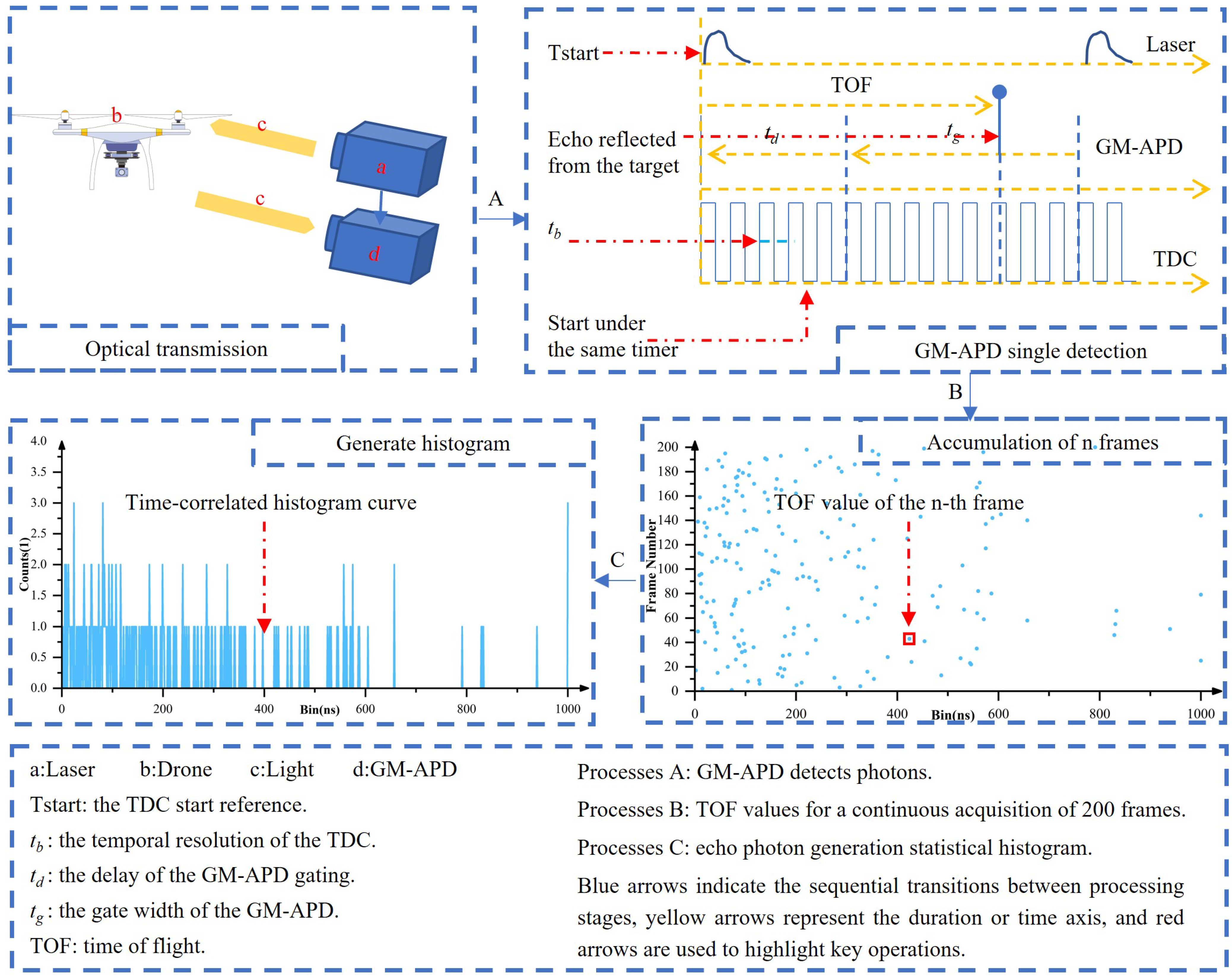
As illustrated in Figure 1, GM-APD LiDAR emits laser pulses at 1064 nm, which are scattered when encountering small targets such as drones, and the GM-APD subsequently collects the scattered photons. During a single detection, the system operates in time-correlated single-photon counting (TCSPC) mode, as shown in Process A. The laser and the GM-APD are synchronized under the time-to-digital converter (TDC) clock. Simultaneously with pulse emission, the GM-APD opens its gate after a delay $t_d$. Operating in synchronized mode, the detector remains active for a gating duration $t_g$, while the TDC provides a temporal resolution of $t_b$. The TDC records the corresponding arrival time when a return photon triggers an avalanche event. Process B records the time-of-flight (TOF) values from 200 consecutively acquired frames. The vertical axis represents the index of consecutive frames, and the horizontal axis denotes the TOF of the current frame. Process C illustrates how repeated gating accumulates the arrival times of return photons, thereby generating statistical echo signals. A histogram is constructed by collecting a fixed number of frames, where the horizontal axis represents the time bin within the gating window and the vertical axis denotes the photon counts. Processing this histogram enables the extraction of key target information, including depth and relative reflectivity. The depth is derived from the timing of photon arrivals, which reflects the distance between the detector and the target. In contrast, reflectivity is a relative measure indicating the strength of the scene’s photon reflection capability.

For a single detection of the individual pixel, assuming the impulse response function (IRF) is Equation (1),

$$g\left(t\right)=N_0{\displaystyle \frac{t}{{\tau }^2}}exp\left[-\left({\displaystyle \frac{t}{\tau }}\right)\right]$$

(1)

where $N_0$ denotes the number of photons emitted by the laser, and $\tau$ represents the laser pulse width.

After a delay of ‘Tdelay,’ the gate’s ‘Tgate’ opens, awaiting the arrival of photons. The probability of the nth bin being triggered under the long dead-time mode is [4,9,24]

$$h_m\left[n\right]\sim \phi \left(n_t|\eta \left({\int }_{n\mathrm{\Delta }t}^{(n+1)\mathrm{\Delta }t}r·g\left(t-{\displaystyle \frac{2z}{c}}\right)dt+n_t\right)\right)$$

(2)

$$n_t=\eta n_a+\eta n_n+n_{da}$$

(3)

In Equations (2) and (3), $\eta$ represents the photon transmission efficiency, r is reflectivity, n is pulsed laser pulse number, $\phi$ follows a Poisson distribution, z is the target distance, c is the speed of light, $n_a$ represents ambient noise photon number, $n_n$ denotes neighboring noise photon number, and $n_{da}$ is the dark count.

2.2. PCA Algorithm Principle

During feature preprocessing, PCA was employed for dimensionality reduction. PCA, as a fundamental data processing technique in LiDAR signal analysis, has been extensively applied for feature extraction and dimensionality reduction. Previous studies have shown that incorporating PCA into LiDAR SLAM can significantly enhance mapping accuracy and overall robustness while maintaining real-time performance [25]. In addition, adaptive PCA-based clustering methods have been proposed to project 3D LiDAR point clouds into lower-dimensional subspaces, enabling efficient noise filtering and fine structural detail preservation, thereby improving both precision and computational efficiency [26]. Furthermore, PCA-based data fusion approaches have proven effective in integrating LiDAR structural features with multispectral information, achieving up to 95% classification accuracy in forest disturbance assessment using UAV LiDAR and multispectral datasets [27]. In GM-APD single-photon LiDAR applications, PCA is commonly employed for data preprocessing. By extracting principal components and analyzing the directional features of target echo signals, PCA enables accurate attitude estimation and dimensionality reduction, thereby improving tracking stability and computational efficiency [28].

In this paper, the MC simulations used a gating window of 1 μs with a temporal resolution of 1 ns, yielding 1000 bins. After excluding the final bin (tail data bin) in the gating window, the original feature dimensionality was 999. PCA was then applied to this feature space, with the number of components determined by preserving 95% of the cumulative explained variance. The retained dimensionalities under different SFNs are summarized in

Table 1. Dimensionality of features before and after PCA under different SFNs.

Frame Count	100	400	800	1000	2000	5000	10,000	20,000
$d=1000$	370	122	17	2	1	1	1	1
$d=999$	657	596	530	503	400	243	126	63

. As shown, fewer statistical frames required more components to achieve the same explained variance, indicating that sparser data contain less effective feature information. No additional hyperparameter optimization, such as cross-validation for component selection, was conducted at this stage and will be considered in future work.

2.3. ML Model Principle

To investigate the applicability and performance of ML algorithms in classifying targets and background noise within GM-APD echo signals, this study evaluates six representative classifiers: DT, LDA, NN-BP, SVM, KNN, and LR. These algorithms exhibit respective advantages in feature extraction, nonlinear modeling, and generalization capabilities, making them suitable for complex scenarios characterized by high noise levels, nonlinear feature distributions, and limited training samples, which are commonly observed in GM-APD signal echoes. Their classification performance is evaluated through experiments, providing insights into algorithm selection and system design for GM-APD-based applications. A detailed description of each algorithm is presented as follows.

2.3.1. DT

The DT algorithm constructs a hierarchical tree structure by recursively partitioning the feature space based on information gain or Gini impurity. Each internal node represents a decision rule on a feature, and each leaf node corresponds to a predicted class. DT can model nonlinear decision boundaries and capture feature interactions without requiring data normalization. Its structure makes it suitable for analyzing the discriminative characteristics of GM-APD echo signals. Previous studies have successfully applied the DT algorithm to airborne LiDAR target extraction tasks, demonstrating its efficiency and interpretability in complex scenes [29]. However, it may suffer from overfitting when applied to small or noisy datasets. Information Gain is a fundamental criterion for determining the optimal attribute to split nodes when constructing a DT.

$$IG(D,A)=Ent\left(D\right)-\sum _{v\in \mathrm{Values}\left(A\right)}{\displaystyle \frac{|D_v|}{\left|D\right|}}·Ent\left(D_v\right)$$

(4)

where $Ent\left(D\right)=-{\sum }_{k=1}^K{p}_k{log}_2{p}_k$ is the entropy of dataset D, and $D_v$ is the subset where attribute A takes value v. This formula is used for attribute selection in DT.

2.3.2. LDA

LDA is a linear classification method that projects high-dimensional data onto a lower-dimensional space where class separability is maximized. It assumes that the data from each class follows a Gaussian distribution with the same covariance matrix. LDA is particularly effective when class distributions are approximately linear, and the number of training samples is limited. Previous studies have demonstrated that LDA is effective for LiDAR-based target classification tasks. For instance, it has been successfully applied to distinguish buildings from non-building planar surfaces in vegetated urban areas, achieving an accuracy of up to 95% [30]. In GM-APD signal classification, LDA can reduce feature dimensionality while preserving class-discriminative information, thus improving computational efficiency and classification robustness. The principle of LDA is based on maximizing the ratio of between-class scatter to within-class scatter.

$$w^{*}=arg\underset{w}{max}{\displaystyle \frac{w^T{S}_{B}w}{w^T{S}_{W}w}}$$

(5)

where $S_B$ and $S_W$ represent the between-class and within-class scatter matrices, respectively. This objective is used in LDA to maximize class separability.

2.3.3. NN-BP

The NN-BP model is a multilayer feed-forward network trained using error backpropagation. It consists of input, hidden, and output layers and uses gradient descent to minimize the loss function. NN-BP have been increasingly applied to LiDAR signal processing, particularly for photon-counting point cloud denoising and classification. Recent studies have demonstrated that NN-BP-based models can effectively suppress background noise and improve the accuracy of interpreting single-photon LiDAR data, achieving F-scores up to 0.977 under strong noise conditions [31].

NN-BP can approximate complex nonlinear relationships between features and class labels, making it suitable for GM-APD signals with highly nonlinear characteristics and noise interferences. Its performance largely depends on network structure, learning rate, and training sample size. We also used NN-BP with dual-layer (NN-BP-2) and triple-layer (NN-BP-3) structures. The core update rule in the error backpropagation algorithm, typically implemented via gradient descent, is formulated as follows:

$$w_{ij}^{(t+1)}=w_{ij}^{\left(t\right)}-\eta ·{\displaystyle \frac{\partial E}{\partial w_{ij}}}$$

(6)

This is the weight update rule in NN-BP neural networks, where $\eta$ is the learning rate, and ${\displaystyle \frac{\partial E}{\partial w_{ij}}}$ is the gradient of the loss function with respect to weight $w_{ij}$.

2.3.4. SVM

SVM is a supervised learning model that seeks to find the optimal hyperplane that maximizes the margin between different classes. For nonlinearly separable data, SVM utilizes kernel functions to map the input space into a higher-dimensional space where linear separation is possible. SVM performs well on high-dimensional and small-sample-size datasets and is robust to noise and outliers. In single-photon LiDAR applications, SVM-based classifiers have been employed to distinguish target and background photons, effectively reducing boundary blur and improving depth reconstruction accuracy [32]. These characteristics make it an appropriate choice for classifying GM-APD echo signals with limited annotated data and complex background interference. In this paper, we considered three kernel functions for SVM-L (Linear), SVM-2 (quadratic), and SVM-3 (cubic). The optimal hyperplane in SVM is obtained by solving the following constrained optimization problem:

$$\underset{\mathbf{w},b}{min}{\displaystyle \frac{1}{2}}{\parallel \mathbf{w}\parallel }^2\mathrm{subject}\mathrm{to}{y}_i({\mathbf{w}}^T{\mathbf{x}}_i+b)\ge 1$$

(7)

This is the primal form of the SVM optimization problem for finding the maximum-margin hyperplane.

2.3.5. KNN

KNN is a non-parametric, instance-based learning algorithm that classifies a sample based on the majority class of its K nearest neighbors in the feature space. It does not require a training phase, which makes it simple to implement. KNN is effective when the samples of each class are locally clustered, and the feature space is well-represented. In photon-counting LiDAR, KNN-based methods distinguish target photons from background noise by analyzing local Euclidean distances, achieving F-scores of 0.97–0.99 across varying noise levels [33]. In the context of GM-APD signal classification, KNN can leverage the similarity of local feature patterns to distinguish between target and background responses. The Euclidean distance formula, commonly used in KNN, is expressed as:

$$d(x,x_i)=\sqrt{\sum _{j=1}^n{(x_j-x_{ij})}^2}$$

(8)

The Euclidean distance used in the KNN algorithm to measure similarity between test sample x and training sample $x_i$.

2.3.6. LR

LR is a linear probabilistic model used for binary classification. It models the relationship between input features and the probability of a class using the logistic sigmoid function. Despite its simplicity, LR provides robust performance when the data exhibits a linear decision boundary. Additionally, LR outputs class probabilities, which can be helpful for confidence-based post-processing. Recent studies have shown that LR can effectively classify geomorphological features such as sinkholes from LiDAR-derived elevation data, achieving an AUC of 0.90 and demonstrating strong reliability in complex terrain analysis [34]. In GM-APD signal classification, LR is a lightweight baseline method with fast training speed and high interpretability. The sigmoid function is used in LR to model the probability that a given input belongs to the positive class, as defined by:

$$P(y=1|x)={\displaystyle \frac{1}{1+exp(-({\mathbf{w}}^T\mathbf{x}+b))}}$$

(9)

This is the logistic function used in LR to compute the probability of the positive class.

2.4. GM-APD Simulated Dataset

Based on Equation (1), MC simulation was employed to generate photon-level datasets for target and noise pixels. Unlike the fixed SNR configuration used in [5,35], approximately 8000 target echoes and 8000 noise echoes were produced with randomly varying SNR values determined by signal intensity, target distance, and ambient light intensity. These data were split into training and testing sets at a 9:1 ratio. The simulated scenario corresponds to sky-background observation, where detector echoes consist solely of two classes: target echoes and sky-background noise echoes.

Table 2. Simulation parameters for target and noise signal generation.

Parameter Category	Parameter Name	Distribution/Range	Description
arget pixels	Noise photons	Uniform [0.01, 1.01]	Simulated background-noise photon count
	Laser photons	Uniform [0.01, 10.01]	Simulated laser-echo photon count
	Target location	Uniform [1, 900]	Time/space index of the target
	Temporal profile of Laser pulse	See Equation (1)	Temporal distribution of the laser pulse
	Laser pulse width $\tau$	Fixed at 20 bins	Constant pulse width
Noise pixels	Noise photons	Uniform [0.01, 1.01]	Simulated pure-noise pixel photon count
GM-APD parameters	Dark count rate	Fixed at 0.01	Dark count rate within the time-gating window
	$T_g$ width	1 μs	Gate width in the synchronous mode of GM-APD
	$T_b$	1 ns	Time resolution within the GM-APD gate

summarizes the simulation parameters, which include photon counts for background noise and laser echoes, target location, temporal characteristics of the laser pulse, and the dark count rate within the time-gating window. Different configurations are specified for target and noise pixels to reproduce signal and background conditions realistically under natural environments. In the present simulation, only clear-weather conditions are considered; factors such as cloud cover and fog, which can affect laser transmission, are not included. The simulation process models the laser and background-light echoes arriving at the target surface, independent of target reflectivity, and generates target laser echoes with varying SNRs.

2.5. Temporal Tail Data

When GM-APD operates in long dead-time mode, especially under low light conditions, it forms a tail peak due to many untriggered events.

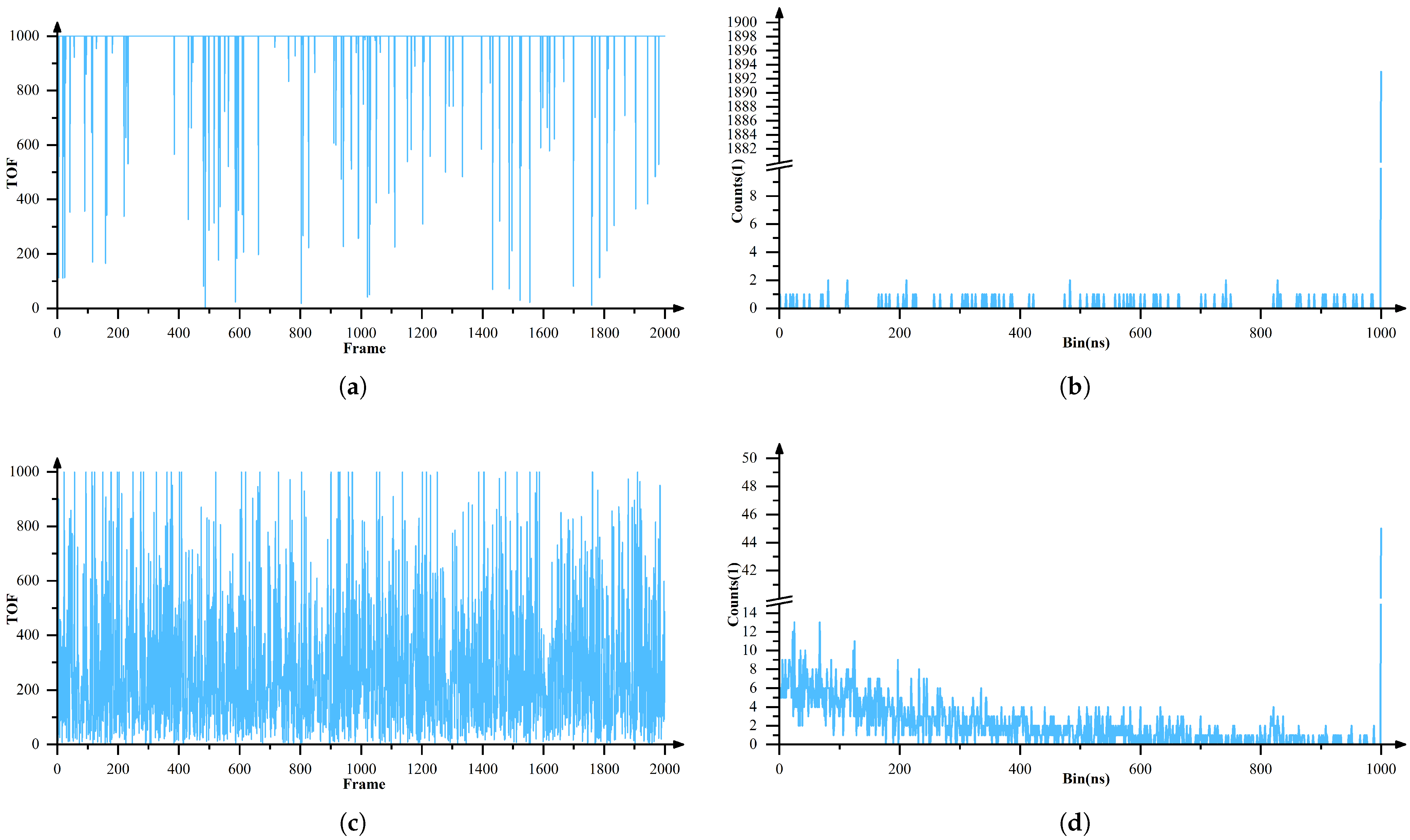
For a specified number of frames, histograms are constructed by accumulating photon-triggered events. Owing to the inherent triggering characteristics of GM-APD detectors, if no avalanche event occurs within a frame, the recorded value defaults to the last time bin of the gating window. Because non-triggering events occur frequently, the accumulated histogram—where the horizontal axis denotes the time bins within the gating window and the vertical axis represents the counts in each bin—exhibits a distinct tail peak at the end of the window. This study defines these data as tail data confined to the final few bins. In the MC simulations, this corresponds to the last bin of the gating window. As illustrated in Figure 2b,d, both background noise and target echoes produce such tail peaks at the end of their histograms. From a detector perspective, this phenomenon is further influenced by the readout circuitry, which forces untriggered events into the final bins. Consequently, the tail data possess highly distinctive characteristics, making them relatively easy to identify and filter.

Rather than discarding the tail peak, we treat it as an explicit feature and examine its impact on classification results.

2.6. Algorithm Principle

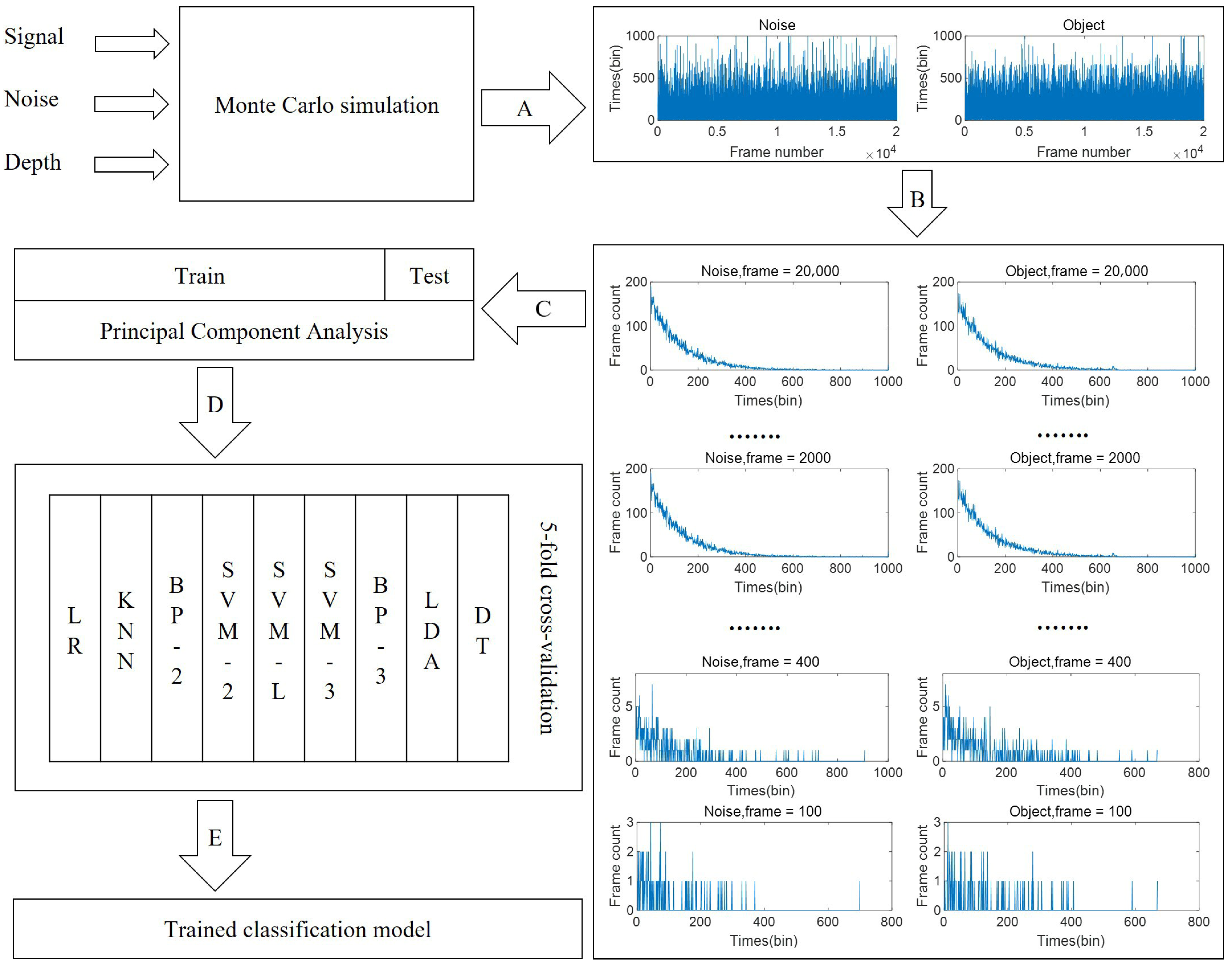
As shown in Figure 3, the simulated dataset is produced by a three-stage pipeline (processes A–C) and then used for model development (processes D–E). In process A, scene parameters and photon statistics are sampled to synthesize target and background echoes. Process B aggregates consecutively acquired frames to form per-frame histograms/features, and process C assigns labels and compiles the final training/testing sets. Before feeding data to the classifiers, we apply PCA to extract low-dimensional, decorrelated features and mitigate noise. Model training (process D) is conducted with stratified five-fold cross-validation to avoid data leakage and to obtain robust estimates. Each fold uses identical preprocessing parameters learned from the training split only, and the procedure is repeated across all folds. Process E performs final fitting on the complete training data and evaluates the selected model on the held-out test set, ensuring a fair, reproducible assessment under the same preprocessing and hyperparameter settings.

2.7. Model Evaluation Metrics

This study employs several metrics to comprehensively evaluate and compare model performance and accuracy, including accuracy, precision, recall, FPR, FNR, F1-score, Kappa coefficient, and RCP. The specific calculations are as follows:

$$Acc={\displaystyle \frac{T_P+T_N}{T_P+T_N+F_P+F_N}}$$

(10)

$$Pre={\displaystyle \frac{T_P}{T_P+F_P}}$$

(11)

$$Rec={\displaystyle \frac{T_P}{T_P+F_N}}$$

(12)

$$FPR={\displaystyle \frac{F_P}{F_P+T_N}}$$

(13)

$$FNR={\displaystyle \frac{F_N}{F_N+T_P}}$$

(14)

$$F1=2·{\displaystyle \frac{Pre\times Rec}{Pre+Rec}}$$

(15)

$$Kapp={\displaystyle \frac{Acc-p_e}{1-p_e}}$$

(16)

$$p_e={\displaystyle \frac{a_1·b_1+a_2·b_2}{N·N}}$$

(17)

$${\delta }_{i,N}=\left|{\displaystyle \frac{Ac{c}_{test}-Ac{c}_{train}}{Ac{c}_{train}}}\right|\times 100\%$$

(18)

The physical meanings of $T_P$, $F_P$, $F_N$, and $T_N$ are provided in

Table 3. Illustration of the confusion matrix.

	Positive (Target)	Negative (Background)
Predicted positive	$T_P$	$F_P$
Predicted negative	$F_N$	$T_N$

. Assuming the actual number of samples for each class is $a_1$ and $a_2$, the predicted number of each class is $b_1$ and $b_2$.

3. Experimental and Results Analysis

3.1. Performance Under Different Feature Extraction Methods

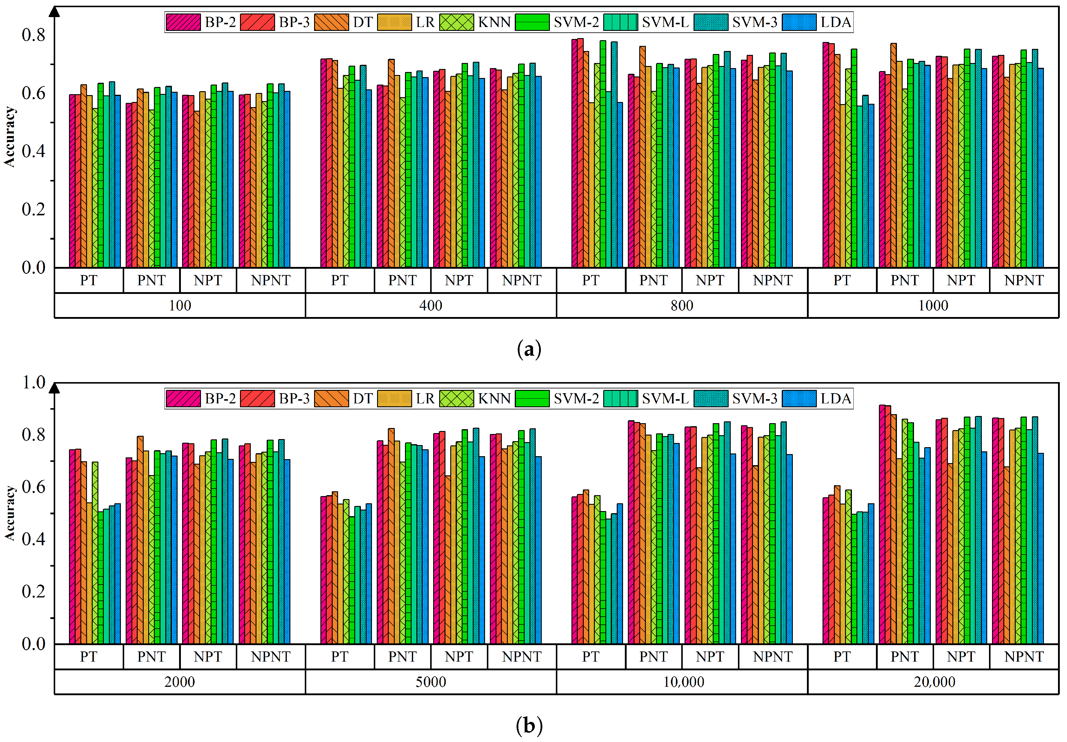
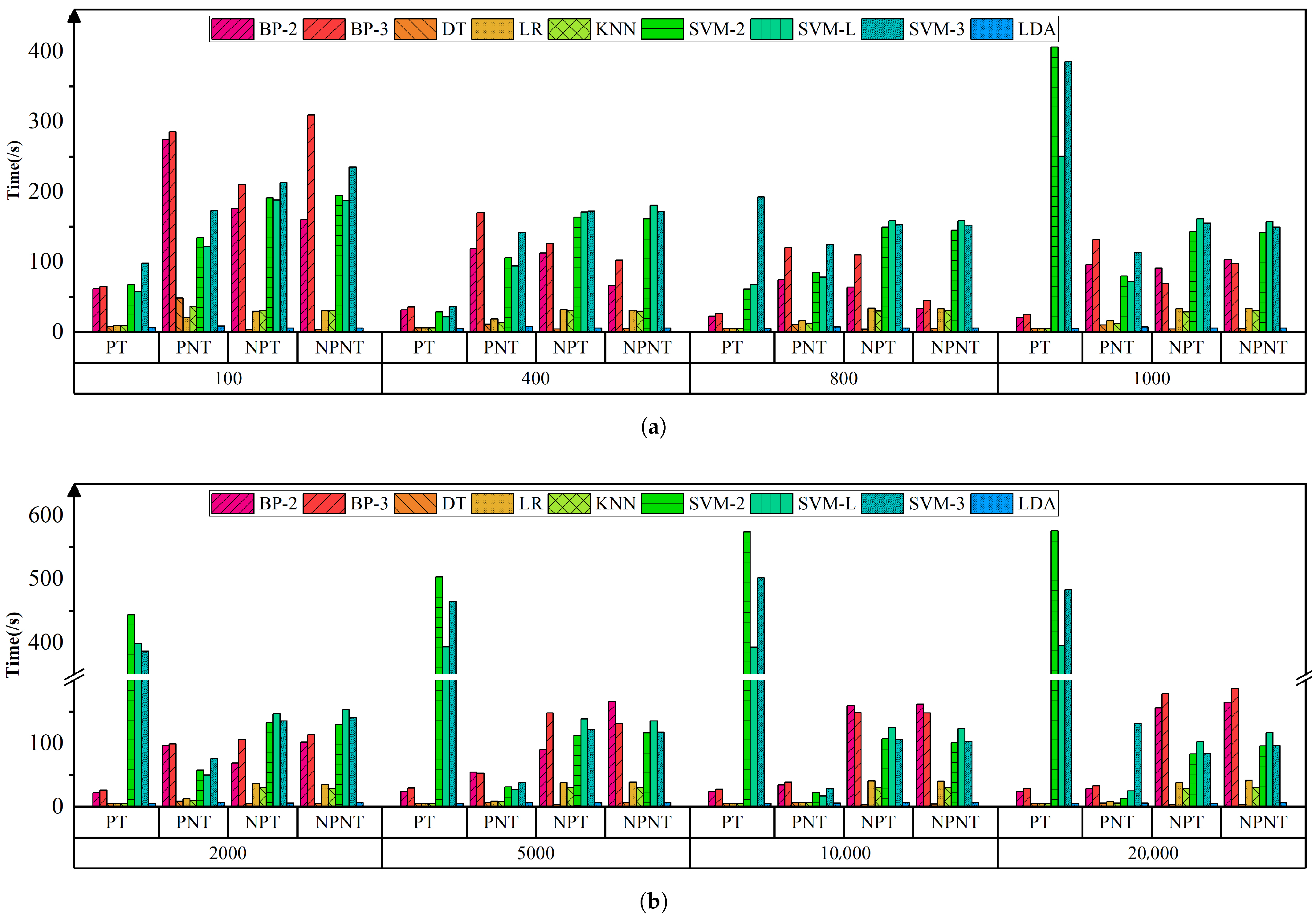
This study conducts an in-depth investigation into the impact of four feature-processing strategies, defined by whether PCA is applied (P vs. NP) and whether tail-end features are retained (T vs. NT). Accordingly, four data-preprocessing schemes are formed: PT, NPT, PNT, and NPNT. Figure 4 provides a detailed representation of the ML models’ performance under different feature processing strategies and SFNs. First, from an accuracy perspective, as the SFN exceeds 2000 frames, the accuracy of models processed with the PNT gradually surpasses that of others. Second, regarding training time, appropriate strategies like PNT can effectively reduce the duration, as depicted in Figure 5, where models based on the PNT feature processing method tend to have shorter training times across different SFNs.

Empirical observations indicate that the tail data do not yield a meaningful improvement in classification performance. The underlying reason is that the discriminative power of GM-APD echoes primarily lies in the local waveform characteristics around the target-return region. In this study, we adopt per-sample normalization to emphasize these local patterns. However, when the tail values are disproportionately large, they shift the global scaling and cause the normalized distribution to be dominated by tail features, thereby suppressing the representation of other salient cues. Consequently, the model’s feature extraction becomes constrained and fails to capture the informative characteristics of the target-return segment effectively. Hence, although the tail segment can be regarded as an independent feature, it does not substantively enhance the overall classification capability.

In summary, PNT emerges as the optimal feature-processing strategy. Thus, we mainly focus on it in the subsequent analysis.

3.2. Performance Analysis Under Different SFNs

In the subsequent research, we explore ML algorithms’ accuracy under different SFNs. SFN significantly impacts the sparsity of GM-APD signals. As illustrated in

Table 4. Sparsity of data at different SFNs.

Frame Count	100	400	800	1000	2000	5000	10,000	20,000
ADNZE	0.0791	0.2270	0.3415	0.3823	0.5137	0.6752	0.7711	0.8409

, we utilize the average density of non-zero elements [36] (ADNZE) to evaluate the sparsity of the echo signal. When the SFN is 100, the ADNZE is 0.0791, increasing to 0.8409 when the SFN rises to 20,000. As the SFN grows, the feature information of the GM-APD signals becomes progressively richer.

Combining the data analysis of Figure 4 and

Table 5. Models with the highest training accuracy and testing accuracy at different SFNs.

Frame Count	100	400	800	1000	2000	5000	10,000	20,000
Train Max	SVM-3	DT-2	DT-2	DT-2	DT-2	NN-BP-2	NN-BP-2	NN-BP-2
Acc	0.6241	0.7171	0.7621	0.7715	0.7947	0.8247	0.8540	0.9137
Train Min	KNN-4	KNN-4	KNN-4	KNN-4	KNN-4	KNN-4	KNN-4	LR-4
Acc	0.5433	0.5852	0.6070	0.6156	0.6453	0.6962	0.7401	0.7091
Test Max	SVM-3	SVM-3	SVM-3	DT-2	DT-2	DT-2	NN-BP-2	NN-BP-3
Acc	0.6219	0.6756	0.7194	0.7662	0.7919	0.8056	0.8681	0.9213
Test Min	KNN-4	KNN-4	KNN-4	KNN-4	KNN-4	KNN-4	KNN-4	LDA-4
Acc	0.5300	0.5669	0.5944	0.5981	0.6294	0.6319	0.7281	0.7538

, we observe that as SFN increases, the accuracy of most models shows an upward trend. For instance, when the SFN is 100, the NN-BP-2 achieves the highest training accuracy of 0.6259; When the SFN increases to 20,000, the NN-BP-2’s training accuracy rises to 0.9137, becoming the highest. Furthermore, as observed in

Table 6. Corresponding metrics for the test data at higher SFNs (100–1000).

Frame Count	Model	Acc	Pre	Rec	FPR	FNR	F1	Kappa
100	NN-BP-3	0.5575	0.5523	0.6075	0.4925	0.4361	0.5786	0.1150
	NN-BP-2	0.5618	0.5613	0.5663	0.4425	0.4376	0.5638	0.1238
	DT	0.5998	0.8272	0.2513	0.0525	0.4414	0.3854	0.1988
	KNN	0.53	1	0.06	0	0.4845	0.1132	0.06
	LR	0.6094	0.6122	0.6013	0.3825	0.3924	0.6062	0.2188
	SVM-2	0.6131	0.6238	0.57	0.3438	0.3959	0.5957	0.2263
	SVM-3	0.6219	0.633	0.58	0.3363	0.3875	0.6053	0.2438
	SVM-L	0.6025	0.6085	0.575	0.37	0.4028	0.5913	0.205
	LDA	0.6088	0.6107	0.6	0.3825	0.3931	0.6053	0.2175
400	NN-BP-3	0.625	0.6312	0.6013	0.3513	0.3807	0.6159	0.25
	NN-BP-2	0.6375	0.6455	0.61	0.335	0.3697	0.6272	0.275
	DT	0.6931	0.9452	0.41	0.0238	0.3767	0.5719	0.3863
	KNN	0.5669	1	0.1338	0	0.4642	0.2359	0.1338
	LR	0.6638	0.6747	0.6325	0.305	0.3459	0.6529	0.3275
	SVM-2	0.6738	0.7087	0.59	0.2425	0.3512	0.6439	0.3475
	SVM-3	0.6756	0.7069	0.6	0.2488	0.3474	0.6491	0.3513
	SVM-L	0.6681	0.6881	0.615	0.2788	0.348	0.6495	0.3363
	LDA	0.6662	0.6817	0.6238	0.2913	0.3468	0.6514	0.3325
800	NN-BP-3	0.6525	0.6506	0.6588	0.3538	0.3456	0.6547	0.305
	NN-BP-2	0.6769	0.6724	0.69	0.3363	0.3184	0.6811	0.3538
	DT	0.7563	0.9702	0.5288	0.0163	0.3239	0.6845	0.5125
	KNN	0.5944	1	0.1888	0	0.4479	0.3176	0.1888
	LR	0.7181	0.733	0.6863	0.25	0.2949	0.7088	0.4363
	SVM-2	0.7187	0.7589	0.6413	0.2038	0.3106	0.6951	0.4375
	SVM-3	0.7194	0.7489	0.66	0.2213	0.3039	0.7017	0.4388
	SVM-L	0.7119	0.7432	0.6475	0.2238	0.3123	0.6921	0.4238
	LDA	0.7025	0.7225	0.6575	0.2525	0.3142	0.6885	0.405
1000	NN-BP-3	0.675	0.6724	0.6825	0.3325	0.3223	0.6774	0.35
	NN-BP-2	0.6613	0.6633	0.655	0.3325	0.3407	0.6591	0.3225
	DT	0.7663	0.9494	0.5625	0.03	0.3108	0.7064	0.5325
	KNN	0.5981	0.9937	0.1975	0.0013	0.4455	0.3295	0.1963
	LR	0.7138	0.728	0.6825	0.255	0.2988	0.7045	0.4275
	SVM-2	0.715	0.7567	0.6338	0.2038	0.3151	0.6898	0.43
	SVM-3	0.7056	0.7031	0.6525	0.2413	0.3141	0.6891	0.4113
	SVM-L	0.715	0.7457	0.6525	0.2225	0.3089	0.696	0.43
	LDA	0.7031	0.7254	0./6538	0.2475	0.3151	0.6877	0.4063
2000	NN-BP-3	0.7006	0.7004	0.7013	0.3	0.2991	0.7008	0.4013
	NN-BP-2	0.7038	0.6993	0.7150	0.3075	0.2916	0.707	0.4075
	DT	0.7919	0.9587	0.61	0.0263	0.286	0.7456	0.5838
	KNN	0.6294	0.9641	0.2688	0.01	0.4248	0.4203	0.2588
	LR	0.7506	0.7684	0.7175	0.2163	0.2649	0.7421	0.5013
	SVM-2	0.735	0.7866	0.645	0.175	0.3008	0.7088	0.47
	SVM-3	0.72	0.7596	0.6438	0.2038	0.3091	0.6969	0.44
	SVM-L	0.7419	0.7945	0.6525	0.1688	0.2948	0.7165	0.4838
	LDA	0.7288	0.774	0.6463	0.1888	0.3036	0.7044	0.4575
5000	NN-BP-3	0.7844	0.792	0.7713	0.2025	0.2229	0.7815	0.5688
	NN-BP-2	0.7931	0.795	0.79	0.2038	0.2087	0.7925	0.5863
	DT	0.8056	0.9358	0.6563	0.045	0.2647	0.7715	0.6113
	KNN	0.6819	0.9619	0.3788	0.015	0.3868	0.5435	0.3638
	LR	0.7925	0.8154	0.7563	0.1713	0.2273	0.7847	0.585
	SVM-2	0.7619	0.8006	0.6975	0.1738	0.268	0.7455	0.5238
	SVM-3	0.7438	0.7671	0.7	0.2125	0.2759	0.732	0.4875
	SVM-L	0.7838	0.8834	0.6538	0.0863	0.2748	0.7514	0.5675
	LDA	0.7556	0.819	0.6563	0.145	0.2868	0.7287	0.5113

and

Table 7. Corresponding metrics for the test data at higher SFNs (2000–20,000).

Frame Count	Model	Acc	Pre	Rec	FPR	FNR	F1	Kappa
2000	NN-BP-3	0.7006	0.7004	0.7013	0.3	0.2991	0.7008	0.4013
	NN-BP-2	0.7038	0.6993	0.7150	0.3075	0.2916	0.707	0.4075
	DT	0.7919	0.9587	0.61	0.0263	0.286	0.7456	0.5838
	KNN	0.6294	0.9641	0.2688	0.01	0.4248	0.4203	0.2588
	LR	0.7506	0.7684	0.7175	0.2163	0.2649	0.7421	0.5013
	SVM-2	0.735	0.7866	0.645	0.175	0.3008	0.7088	0.47
	SVM-3	0.72	0.7596	0.6438	0.2038	0.3091	0.6969	0.44
	SVM-L	0.7419	0.7945	0.6525	0.1688	0.2948	0.7165	0.4838
	LDA	0.7288	0.774	0.6463	0.1888	0.3036	0.7044	0.4575
5000	NN-BP-3	0.7844	0.792	0.7713	0.2025	0.2229	0.7815	0.5688
	NN-BP-2	0.7931	0.795	0.79	0.2038	0.2087	0.7925	0.5863
	DT	0.8056	0.9358	0.6563	0.045	0.2647	0.7715	0.6113
	KNN	0.6819	0.9619	0.3788	0.015	0.3868	0.5435	0.3638
	LR	0.7925	0.8154	0.7563	0.1713	0.2273	0.7847	0.585
	SVM-2	0.7619	0.8006	0.6975	0.1738	0.268	0.7455	0.5238
	SVM-3	0.7438	0.7671	0.7	0.2125	0.2759	0.732	0.4875
	SVM-L	0.7838	0.8834	0.6538	0.0863	0.2748	0.7514	0.5675
	LDA	0.7556	0.819	0.6563	0.145	0.2868	0.7287	0.5113
10,000	NN-BP-3	0.8494	0.8625	0.8313	0.1325	0.1628	0.8466	0.6988
	NN-BP-2	0.8681	0.887	0.8438	0.1075	0.149	0.8648	0.7363
	DT	0.8444	0.9599	0.7188	0.03	0.2248	0.822	0.6888
	KNN	0.7281	0.8585	0.5463	0.09	0.3327	0.6677	0.4563
	LR	0.8031	0.8392	0.75	0.1438	0.226	0.7921	0.6063
	SVM-2	0.8125	0.9098	0.6938	0.0688	0.2475	0.7872	0.625
	SVM-3	0.8125	0.8776	0.7263	0.1013	0.2335	0.7948	0.625
	SNM-L	0.8006	0.9168	0.6613	0.06	0.2649	0.7683	0.6013
	LDA	0.7781	0.887	0.6375	0.0813	0.2829	0.7418	0.5563
20,000	NN-BP-3	0.9213	0.947	0.8925	0.050	0.1017	0.9189	0.8425
	NN-BP-2	0.9188	0.9385	0.8963	0.0588	0.0993	0.9169	0.8375
	DT	0.8681	0.9712	0.7588	0.0225	0.1979	0.8519	0.7363
	KNN	0.8731	0.9222	0.815	0.0688	0.1657	0.8653	0.7463
	LR	0.7706	0.8442	0.6638	0.1225	0.277	0.7432	0.5413
	SVM-2	0.8369	1.0000	0.6738	0	0.246	0.8051	0.6738
	SVM-3	0.8488	1.0000	0.6975	0	0.2322	0.8218	0.6975
	SVM-L	0.7675	0.935	0.575	0.04	0.3069	0.7121	0.535
	LDA	0.7538	0.9301	0.5488	0.0413	0.32	0.6903	0.5075

, the evaluation metrics of most algorithms show an upward trend with the increase in SFN. For example, NN-BP-2’s precision increases from 0.5613 to 0.9384 and recall from 0.5662 to 0.8962. Simultaneously, both the FNR and FPR decrease, while the F1-score and kappa coefficient also experience growth, all indicating a significant improvement in model performance. Additionally, the analysis, combined with Table 5, shows that the DT consistently performs well regarding stability and efficiency across different SFNs.

We analyzed F1-score and Kappa across models using the raw F1/Kappa matrices (Table 6 and Table 7) and summarized model-wise means with 95% confidence intervals (

Table 8. Mean ± 95% CI per model (F1/Kappa).

Model	Mean		SD		Lower 95% CI		Upper 95% CI
	F1	Kappa	F1	Kappa	F1	Kappa	F1	Kappa
NN-BP-3	0.7218	0.4414	0.1175	0.2435	0.6236	0.2378	0.8200	0.6450
NN-BP-2	0.7266	0.4553	0.1213	0.2434	0.6251	0.2518	0.8280	0.6589
DT	0.6924	0.5313	0.1514	0.1723	0.5659	0.3872	0.8189	0.6754
KNN	0.4366	0.3005	0.2448	0.2196	0.2320	0.1169	0.6413	0.4841
LR	0.7168	0.4555	0.0634	0.1323	0.6638	0.3449	0.7698	0.5661
SVM-2	0.7089	0.4667	0.0700	0.1441	0.6503	0.3462	0.7674	0.5872
SVM-3	0.7113	0.4619	0.0712	0.1445	0.6518	0.3411	0.7709	0.5827
SVM-L	0.6971	0.4478	0.0562	0.1304	0.6502	0.3388	0.7441	0.5569
LDA	0.6873	0.4242	0.0431	0.1101	0.6512	0.3322	0.7233	0.5163

and

Table 9. Friedman test summary (F1/Kappa).

	Chi-Square		p-Value		Kendall’s W		N (SFN Levels)	k (Models)
	F1	Kappa	F1	Kappa	F1	Kappa
Value	18.83	24.14	0.0158	0.00217	0.29	0.38	8	9

). We applied non-parametric tests because the sample size per model is small (eight SFN levels) and normality is not guaranteed. A Friedman test with SFN as blocks revealed significant overall differences for both F1 (${\chi }^2\left(8\right)=18.83$, $p=0.0158$; Kendall’s $W=0.294$) and Kappa (${\chi }^2\left(8\right)=24.14$, $p=0.0022$; $W=0.377$). The confidence interval results further quantified performance, showing that NN-BP-2, NN-BP-3, and LR achieved the highest mean F1 values (∼$0.72$–$0.73$), while DT and SVM-2 performed best on Kappa (∼$0.47$–$0.53$).

To further examine specific model contrasts, pairwise Wilcoxon signed-rank tests (

Table 10. Pairwise Wilcoxon—all model pairs (F1/Kappa).

Model A	Model B	Mean_Diff		Median_Diff		${\mathit{p}}_{\mathbf{value}}$		${\mathit{p}}_{\mathbf{adj}\_\mathit{holm}}$		Effect_Size_r
		F1	Kappa	F1	Kappa	F1	Kappa	F1	Kappa	F1	Kappa
DT	KNN	0.2558	0.2308	0.2988	0.2500	0.0156	0.0156	0.4531	0.4219	0.855	0.855
DT	LDA	0.0051	0.1070	0.0300	0.1168	0.6406	0.0156	1	0.4688	0.165	0.855
DT	LR	−0.0244	0.0758	−0.0056	0.0793	0.7422	0.0156	1	0.4375	−0.116	0.855
DT	SVM-2	−0.0165	0.0645	0.0213	0.0694	0.8438	0.0156	1	0.5156	0.070	0.855
DT	SVM-3	−0.0189	0.0694	0.0222	0.0687	0.8438	0.0391	1	0.9375	0.070	0.730
DT	SVM-L	−0.0047	0.0834	0.0153	0.0881	0.7422	0.0156	1	0.4531	0.116	0.855
KNN	LDA	−0.2506	−0.1237	−0.3211	−0.1781	0.0234	0.1953	0.6562	1	−0.801	−0.458
KNN	LR	−0.2802	−0.1550	−0.3484	−0.2074	0.0156	0.0547	0.4688	1	−0.855	−0.679
KNN	SVM-2	−0.2723	−0.1662	−0.3244	−0.1900	0.0156	0.0156	0.4844	0.4844	−0.855	−0.855
KNN	SVM-3	−0.2747	−0.1614	−0.3181	−0.1825	0.0156	0.0156	0.5	0.5	−0.855	−0.855
KNN	SVM-L	−0.2605	−0.1473	−0.3313	−0.2031	0.0234	0.0781	0.6328	1	−0.801	−0.623
LR	LDA	0.0295	0.0313	0.0290	0.0326	0.0078	0.0234	0.2734	0.6094	0.940	0.801
LR	SVM-2	0.0079	−0.0112	0.0121	−0.0050	0.1953	0.5469	1	1	0.458	−0.213
LR	SVM-3	0.0055	−0.0064	0.0055	−0.0106	0.3125	0.7422	1	1	0.357	−0.116
LR	SVM-L	0.0197	0.0077	0.0202	0.0094	0.0078	0.0781	0.2656	1	0.940	0.623
NN-BP-2	DT	0.0342	−0.0759	0.0319	−0.0931	0.25	0.1094	1	1	0.407	−0.566
NN-BP-2	KNN	0.2899	0.1548	0.3081	0.1450	0.0078	0.0078	0.2578	0.2656	0.940	0.940
NN-BP-2	LDA	0.0393	0.0311	−0.0024	−0.0506	0.6406	0.9453	1	1	−0.165	−0.024
NN-BP-2	LR	0.0097	−0.0002	−0.0267	−0.0675	0.8438	0.8438	1	1	−0.070	−0.070
NN-BP-2	SVM-2	0.0177	−0.0114	−0.0079	−0.0675	0.7422	0.9453	1	1	−0.116	−0.024
NN-BP-2	SVM-3	0.0152	−0.0066	−0.0052	−0.0544	0.6406	0.9453	1	1	−0.165	−0.024
NN-BP-2	SVM-L	0.0294	0.0075	−0.0103	−0.0656	0.7422	0.8438	1	1	−0.116	−0.070
NN-BP-3	DT	0.0294	−0.0899	0.0173	−0.1100	0.5469	0.0781	1	1	0.213	−0.623
NN-BP-3	KNN	0.2852	0.1409	0.3088	0.1294	0.0078	0.0078	0.2812	0.2734	0.940	0.940
NN-BP-3	LDA	0.0345	0.0172	−0.0070	−0.0563	0.7422	1	1	1	−0.116	−0.000
NN-BP-3	LR	0.0050	−0.0141	−0.0273	−0.0775	0.7422	0.4609	1	1	−0.116	−0.261
NN-BP-3	NN-BP-2	−0.0048	−0.0139	−0.0086	−0.0132	0.5469	0.1484	1	1	−0.213	−0.511
NN-BP-3	SVM-2	0.0129	−0.0253	−0.0102	−0.0743	0.8438	0.4609	1	1	−0.070	−0.261
NN-BP-3	SVM-3	0.0105	−0.0205	−0.0039	−0.0500	0.6406	0.7422	1	1	−0.165	−0.116
NN-BP-3	SVM-L	0.0247	−0.0064	−0.0142	−0.0813	0.9453	0.7422	1	1	−0.024	−0.116
SVM-2	LDA	0.0216	0.0425	0.0055	0.0193	0.25	0.0078	1	0.2812	0.407	0.940
SVM-2	SVM-3	−0.0024	0.0048	−0.0059	−0.0007	0.6406	0.7263	1	1	−0.165	−0.124
SVM-2	SVM-L	0.0117	0.0189	−0.0013	0.0124	1	0.3627	1	1	−0.000	0.322
SVM-3	LDA	0.0241	0.0377	0.0024	0.0225	0.1834	0.1094	1	1	0.470	0.566
SVM-3	SVM-L	0.0142	0.0141	0.0046	0.0150	0.6406	0.8438	1	1	0.165	0.070
SVM-L	LDA	0.0099	0.0236	0.0102	0.0250	0.1094	0.0234	1	0.5859	0.566	0.801

) indicated that NN-BP-3 vs. KNN yielded p = 0.0078 for both F1 and Kappa before adjustment. Although conservative Holm corrections attenuated these differences (adjusted p > 0.05), bootstrap analysis confirmed their robustness: NN-BP-3 exceeded KNN by 0.285 in F1 [0.200, 0.364] and by 0.141 in Kappa [0.104, 0.181]. These complementary tests ensure that the observed differences are not incidental but reflect meaningful and statistically supported performance gaps. Overall, the results highlight that NN-BP-based models offer a clear and practically relevant advantage over baseline methods such as KNN across SFNs, even if some pairwise contrasts do not survive stringent multiplicity corrections.

3.3. Robust Analysis Under Echo SNR

The target echo signal-to-noise ratio (ESNR) represents the ratio of the target signal to the background signal when the echo arrives at the detector surface. ESNR varies with time and environmental conditions; therefore, evaluating ML performance under different ESNRs is a critical indicator of model classification accuracy and robustness. In this section, we investigate the classification performance of ML models under three representative statistical frame numbers (SFNs: 400, 2000, and 20,000). Here, the number of target echoes and background noise signals is kept consistent, and the statistical distribution of the ESNR of target echoes is used to analyze model performance. The subsequent analysis particularly emphasizes binary classification between low-ESNR target echoes and background noise echoes.

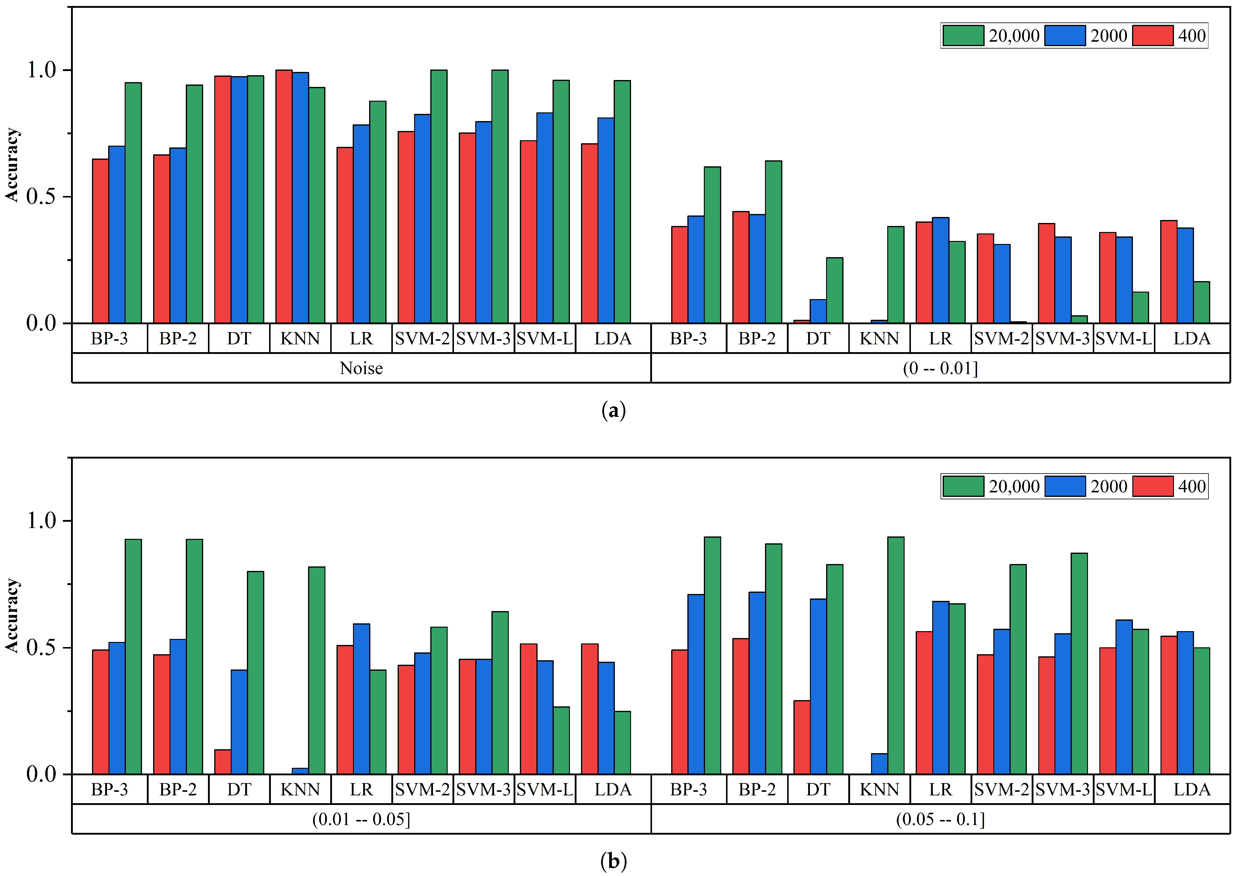
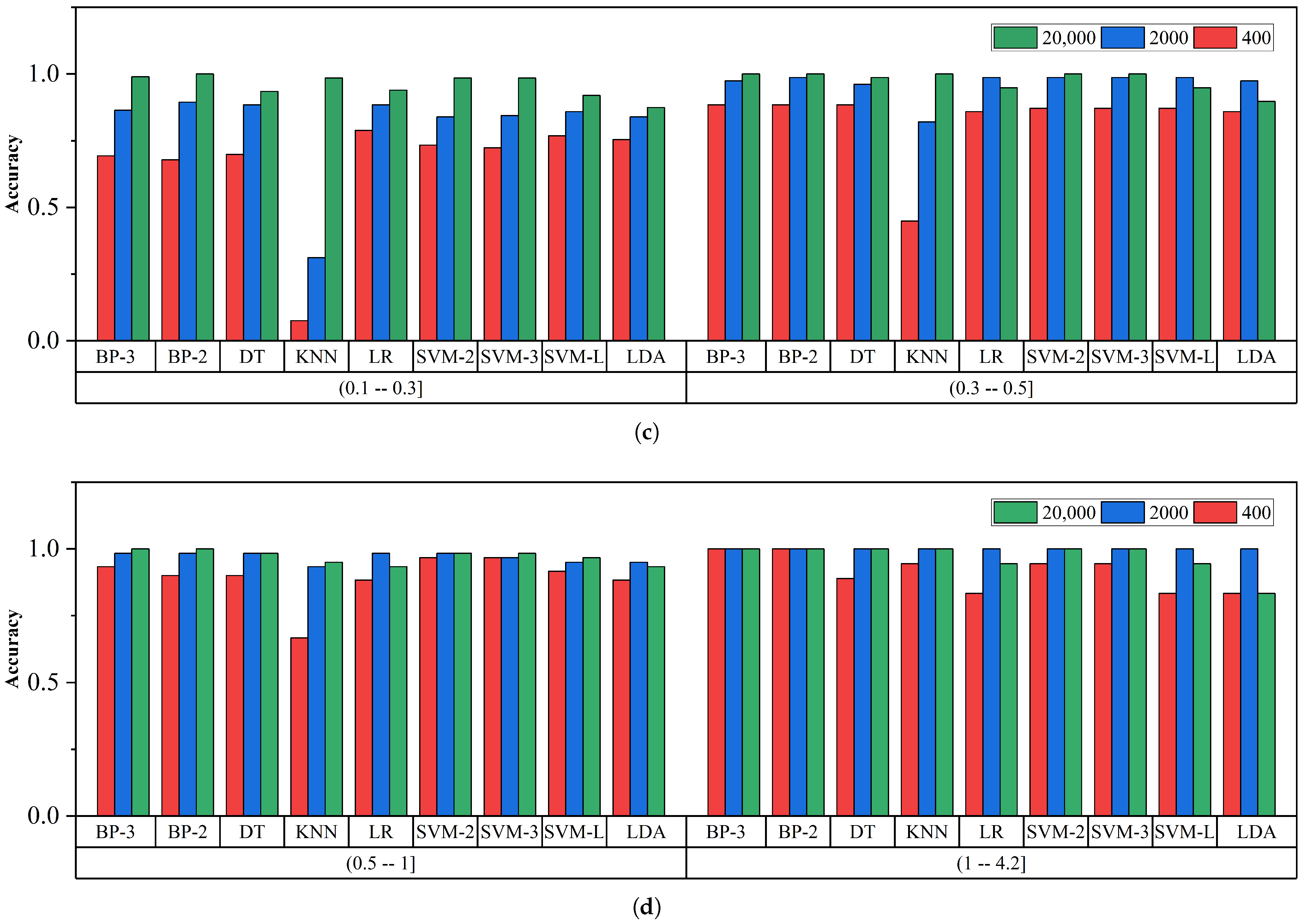
Combining the data analysis of

Table 11. Distribution of different ESNRs in the test data (calculated under SFN being 20,000).

ESNR	Number	Percent (%)
(0.00–0.01]	170	21.25
(0.01–0.05]	165	20.625
(0.05–0.10]	110	13.75
(0.10–0.30]	199	24.875
(0.30–0.50]	78	9.75
(0.50–1.00]	60	7.5
(1.00–4.20]	18	2.25

and Figure 6, we observe that under low ESNR (0–0.1) conditions, the performance of most algorithms declines. However, NN-BP-based algorithms exhibit exceptional performance within the ESNR range of 0–0.05. Under medium ESNR (0.1–0.5) conditions, the performance of algorithms generally improves, with LR and SVM particularly standing out in the ESNR interval of 0.3–0.5, achieving a value close to 1. In high ESNR (above 0.5) environments, the accuracy of all algorithms approaches or reaches 1, indicating that they can effectively handle high SNR data. However, consistent with the conclusion in Section 3.2, when the SFN is relatively low, the ESNR will decrease further, leading to a decline in the classification accuracy of each model. Overall, the NN-BP-based algorithm demonstrates robust performance under various ESNR conditions.

Figure 7 presents the Acc of different models across varying ESNRs under three representative SFNs: (a) SFN = 400, (b) SFN = 2000, and (c) SFN = 20,000. Overall, all models experience a pronounced drop in accuracy at extremely low ESNRs (e.g., ESNR < 0.01), followed by a gradual recovery as ESNR increases. A key turning point is observed when ESNR exceeds approximately 0.05, where BP-based models (NN-BP-2 and NN-BP-3) outperform other algorithms, particularly under the low-SFN scenario shown in Figure 7a. This superiority arises from the nonlinear fitting capacity and multilayer feature representation of NN-BPs, which enable more effective extraction of weak target signals from noisy data. By contrast, linear models such as LDA and LR exhibit limited adaptability, resulting in severe degradation under low-ESNR conditions. As the SFN increases to 2000 and 20,000 (Figure 7b,c), model performance converges, and the advantage of NN-BP-based models diminishes, indicating that larger statistical frames reduce noise sensitivity and mitigate differences across algorithms. These findings demonstrate the coupled influence of ESNR and SFN on classification performance and highlight the suitability of NN-BPs for low-SNR and small-sample scenarios.

3.4. Model Stability Analysis

Figure 8 illustrates the analysis of training accuracy, testing accuracy, and their relative stability for ML models under three different SFNs (400, 2000, 20,000). The smaller the RCP value, the stronger the model’s stability. The results indicate that the NN-BP-3 model exhibits smaller RCP values across all frame counts, especially when SFN is 20,000, where its RCP value is only 0.0111. Conversely, the SVM-3 model has the most significant RCP value of 0.1937 among all models when SFN is 20,000, suggesting lower stability under this condition.

3.5. Lightweight ResNet on NN-BP Backbone: Gain Verification on GM-APD LiDAR Signals

Building on the preceding results, NN-BP-type networks already exhibit a clear advantage for classifying GM-APD LiDAR data. To further test whether an NN-BP backbone can yield additional gains, we augment the NN-BP architecture with 1-D convolutions and residual connections, forming a lightweight ResNet-style model tailored to the temporal characteristics of GM-APD signals.

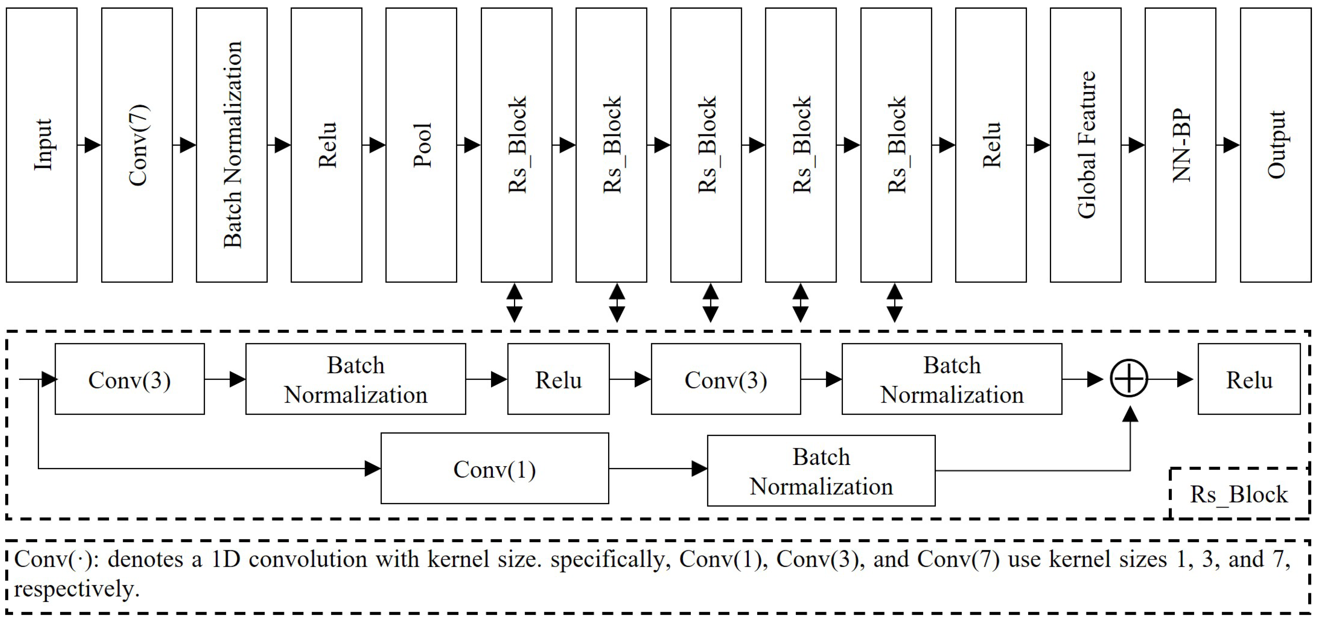
The NN-BP-enhanced ResNet is illustrated in Figure 9. To accommodate the long 1D sequences within the GM-APD gating window, the network first applies Conv(7) + Batch Normalization (BN) + Rectified Linear Unit (ReLU) to capture long-range temporal dependencies, followed by a pooling layer for local noise suppression and mild down-sampling. The backbone then stacks five residual blocks (Rs_Block). In each block, the main branch adopts Conv(3)–BN–ReLU–Conv(3)–BN, while the shortcut branch uses Conv(1)–BN for channel/length alignment; the two branches are summed element-wise and passed through ReLU. This design deepens the network, enlarges the receptive field, and mitigates gradient vanishing without incurring excessive optimization burden. After the backbone, a ReLU and global feature aggregation produce a compact representation, which is finally fed to the NN-BP head for classification output.

Table 12. Performance comparison at different accumulation frame counts on GM-APD echoes.

Frame Count	Model	Acc	Pre	Rec	FPR	FNR	F1	Kappa
400	DT	0.6931	0.9452	0.4100	0.0238	0.3767	0.5719	0.3863
400	ResNet	0.7800	0.8425	0.6887	0.1288	0.3113	0.7579	0.5600
2000	DT	0.7919	0.9587	0.6100	0.0263	0.2860	0.7456	0.5838
2000	ResNet	0.8644	0.9664	0.7550	0.0262	0.2450	0.8477	0.7288
20,000	NN-BP-3	0.9213	0.9470	0.8925	0.0500	0.1017	0.9189	0.8425
20,000	ResNet	0.9444	0.9696	0.9175	0.0288	0.0825	0.9428	0.8887

compares ResNet with the best-performing method in Table 6 and Table 7 at 400, 2000, and 20,000 frames—DT for 400 and 2000 and NN-BP-2 for 20,000. Results show that the NN-BP-based ResNet consistently outperforms the corresponding baselines, with relative improvements of 12.5% (400), 9.16% (2000), and 2.79% (20,000). These findings indicate that introducing convolutional and residual units on top of the NN-BP prior structure captures local and cross-scale patterns in GM-APD signals more effectively, while still providing steady—though diminishing—marginal gains at high frame counts. Accordingly, subsequent work will focus on NN-BP-based architectural optimization, incorporating the physical characteristics of GM-APD signals (e.g., pulse statistics and background-noise signatures) to further enhance robustness in complex spatial backgrounds.

3.6. Model Computational Complexity Analysis

Table 13. Run time and model size comparison at different accumulation frame counts.

Frame Count	M-Name	Algorithm Time (s)	Avg. Latency (ms)	Rate (Hz)	Params (MB)
400	NN-BP-3	0.8536	0.2084	1.1715	2.4100
	NN-BP-2	0.2746	0.0670	3.6417	4.8200
	DT	0.4014	0.0980	2.4913	2.3900
	KNN	3.9585	0.9664	0.2526	36.8400
	LR	0.5453	0.1331	1.8339	2.3880
	SVM-2	4.2910	1.0474	0.2331	29.7200
	SVM-3	4.6212	1.1282	0.2164	31.9170
	SVM-L	3.7983	0.9273	0.2633	27.9180
	LDA	0.3543	0.0865	2.8225	3.8140
	ResNet	6.5561	1.6006	0.1525	0.3800
2000	NN-BP-3	0.2167	0.0529	4.6147	1.6190
	NN-BP-2	0.1942	0.0474	5.1493	1.6190
	DT	0.1323	0.0332	7.5586	1.6070
	KNN	2.7283	0.6661	0.3665	24.7610
	LR	0.1712	0.0418	5.8411	1.6040
	SVM-2	1.6910	0.4129	0.5914	17.1840
	SVM-3	2.0473	0.4998	0.4884	18.6390
	SVM-L	1.7719	0.4326	0.5644	16.4310
	LDA	0.1947	0.0475	5.1361	2.2470
	ResNet	6.9294	1.6918	0.1443	0.3800
20,000	NN-BP-3	0.1444	0.0352	6.9252	0.2588
	NN-BP-2	0.1032	0.0252	9.6899	0.2588
	DT	0.1312	0.0320	7.6220	0.2600
	KNN	0.4405	0.1076	2.2701	4.0000
	LR	0.1711	0.0418	5.8445	0.2560
	SVM-2	0.3407	0.0832	2.9351	1.7530
	SVM-3	0.3049	0.0735	3.2312	1.5290
	SVM-L	0.3491	0.0852	2.8645	2.3970
	LDA	0.1241	0.0303	8.0580	0.2274
	ResNet	7.1379	1.7426	0.1401	0.3800

reports efficiency and model size under the PNT strategy for three representative accumulation frame counts (400, 2000, and 20,000). All metrics are computed on 4096 samples and include the total test time, the average per-sample latency, and the imaging frame rate converted from the total time. Model size is measured in FP32 (4 bytes per parameter) and includes the PCA projection parameters. Note that ResNet does not use PCA, and thus, its parameter count remains unchanged across frame settings.

In terms of efficiency, NN-BP-based models consistently deliver lower latency and higher frame rates across all three accumulation settings. Taking NN-BP-2 as an example, the average per-sample latency is 0.067, 0.047, and 0.025 ms for SFN = 400, 2000, and 20,000, respectively. Assuming 4096 samples constitute one frame (corresponding to a 64 × 64 pixel GM-APD array), these latencies translate to frame rates of 3.64, 5.15, and 9.69 Hz, respectively. Under the same settings, NN-BP-3 attains 1.17, 4.61, and 6.93 Hz. By contrast, ResNet achieves only 0.14–0.15 Hz, indicating that the current convolution–residual stacking is not amenable to real-time processing.

Regarding model size, increasing the frame count does not enlarge the models. Most PCA-based methods become smaller as the frame count rises. For example, the size of NN-BP-2 decreases from 4.820 MB to 1.619 MB and then to 0.259 MB. This is because higher frame counts produce more stable echo statistics and less sparsity, so fewer principal components are needed and the projection matrix becomes smaller. ResNet does not use PCA, so its size remains 0.380 MB across all frame counts.

Taken together with Table 12 and Table 13, although the NN-BP-based ResNet substantially improves accuracy, its computational cost and parameter footprint also increase, resulting in reduced real-time capability. These observations suggest that subsequent work should prioritize efficiency optimization for NN-BP-type networks, for example, by pursuing light-weight architectures, operator fusion, and low-bit quantization while maintaining accuracy.

4. Conclusions

This study proposed a complete data-processing framework for GM-APD LiDAR echo signals and systematically assessed nine ML models derived from six baseline algorithms. Feature extraction was optimized through PCA, and among the candidate schemes, the PNT strategy emerged as the optimal feature-processing method. This framework provides a novel and feasible approach for GM-APD data classification, which, to our knowledge, has not been explicitly formulated in prior work. Building upon this framework, MC simulations were carried out under varying ESNR and SFN conditions. The results showed that NN-BP-based models (NN-BP-2 and NN-BP-3) performed best in low-SNR and small-sample regimes. LR and LDA were fast but less robust, DT achieved good stability, and SVM models yielded competitive accuracy but at a higher computational cost. Building on these findings, we further introduce an NN-BP-based ResNet that achieves additional test-accuracy gains at typical frame counts. Complemented by bootstrap confidence intervals, statistical significance analysis using Friedman and Wilcoxon tests confirmed that the observed differences among models are statistically meaningful.

In addition to accuracy and robustness, practical deployment must also balance computational efficiency and hardware deployability. Lightweight models (LR/LDA) offer the fastest inference and the smallest parameter footprint, making them suitable for embedded or resource-constrained platforms, albeit with limited noise resilience. NN-BP models provide stronger overall accuracy and stability with an acceptable runtime overhead, fitting scenarios that require both real-time performance and high accuracy. By contrast, SVM and KNN incur higher computational and memory costs. Although ResNet attains the highest accuracy, it bears the most significant computational load and the lowest throughput, thus being more appropriate for offline analysis or high-compute platforms. Moreover, empirical timing across models trained with different SFNs shows that increasing SFN reduces sample sparsity, thereby lowering the number of principal components needed by PCA and, paradoxically, improving efficiency for PCA-based methods; SFN has no noticeable effect on ResNet, which does not rely on PCA. Finally, this study considers clear-sky conditions only; more complex atmospheres (e.g., fog or cloud) would further increase the computational burden, underscoring the need to jointly evaluate algorithmic performance, time complexity, memory footprint, and hardware compatibility in real GM-APD systems.

Looking ahead, methodological generalization to real-scene datasets is planned through a staged route encompassing hardware finalization and calibration, multi-scenario data acquisition with standardized and traceable records, ground-truth construction using surveyed references, and protocol/metric standardization for fair comparison. Further directions include cross-dataset generalization and sim-to-real transfer studies, the inclusion of representative deep-learning baselines (e.g., Transformers, MLPs), and the exploration of lightweight or hardware-adaptive solutions (pruning, quantization, operator fusion, on-device deployment) to jointly optimize accuracy, robustness, and computational efficiency. Extending the simulation suite to atmospheric conditions beyond clear weather (e.g., fog, haze, turbulence) will enhance realism. Collectively, these efforts are expected to advance GM-APD LiDAR signal processing toward high-precision, resource-efficient, and real-time applications.

References

1. Zhou, S.L.; Xu, H.; Zhang, G.H.; Ma, T.W.; Yang, Y. Leveraging Deep Convolutional Neural Networks Pre-Trained on Autonomous Driving Data for Vehicle Detection From Roadside LiDAR Data. IEEE Trans. Intell. Transp. Syst. 2022, 23, 22367–22377. [Google Scholar] [CrossRef]
2. Hua, Z.Y.; Xu, S.; Liu, Y.A. Individual Tree Segmentation from Side-View LiDAR Point Clouds of Street Trees Using Shadow-Cut. Remote Sens. 2022, 14, 5742. [Google Scholar] [CrossRef]
3. Li, C.; Cheng, N.; Zhao, H.; Yu, T.C. Multiple-Beam LiDAR Detection Technology. In Proceedings of the Seventh Asia Pacific Conference on Optics Manufacture and 2021 International Forum of Young Scientists on Advanced Optical Manufacturing (APCOM and YSAOM 2021), Hong Kong, 13–16 August 2021; p. 12166. [Google Scholar] [CrossRef]
4. Ma, L.; Sun, J.F.; Jiang, P.; Liu, D.; Zhou, X.; Wang, Q. Signal Extraction Algorithm of Gm-APD LiDAR with Low SNR Return. Optik 2020, 206, 164340. [Google Scholar] [CrossRef]
5. Wang, M.Q.; Sun, J.F.; Li, S.N.; Lu, W.; Zhou, X.; Zhang, H.L. A Photon-Number-Based Systematic Algorithm for Range Image Recovery of GM-APD LiDAR under Few-Frames Detection. Infrared Phys. Technol. 2022, 125, 104267. [Google Scholar] [CrossRef]
6. Zhang, Y.B.; Li, S.N.; Sun, J.F.; Liu, D.; Zhang, X.; Yang, X.H.; Zhou, X. Dual-Parameter Estimation Algorithm for Gm-APD LiDAR Depth Imaging through Smoke. Measurement 2022, 196, 111269. [Google Scholar] [CrossRef]
7. Zhang, X.; Sun, J.; Li, S.; Zhang, Y.; Liu, D.; Zhang, H. Research on the Detection Probability Curve Characteristics of Long-Range Target Based on SPAD Array LiDAR. Infrared Phys. Technol. 2022, 126, 104325. [Google Scholar] [CrossRef]
8. Zhang, X.; Li, S.; Sun, J.; Zhang, Y.; Liu, D.; Yang, X.; Zhang, H. Target Edge Extraction for Array Single-Photon LiDAR Based on Echo Waveform Characteristics. Opt. Laser Technol. 2023, 167, 109736. [Google Scholar] [CrossRef]
9. Liu, D.; Sun, J.F.; Gao, S.; Ma, L.; Jiang, P.; Guo, S.H.; Zhou, X. Single-Parameter Estimation Construction Algorithm for Gm-APD Ladar Imaging through Fog. Opt. Commun. 2021, 482, 126558. [Google Scholar] [CrossRef]
10. Fan, T.; Qiu, S.; Wang, Z.; Zhao, H.; Jiang, J.; Wang, Y.; Zhou, X. A New Deep Convolutional Neural Network Incorporating Attentional Mechanisms for ECG Emotion Recognition. Comput. Biol. Med. 2023, 159, 106938. [Google Scholar] [CrossRef]
11. Khan, F.; Yu, X.; Yuan, Z.; Rehman, A.U. ECG Classification Using 1-D Convolutional Deep Residual Neural Network. PLoS ONE 2023, 18, 284791. [Google Scholar] [CrossRef] [PubMed]
12. Raza, A.; Mehmood, A.; Ullah, S.; Ahmad, M.; Choi, G.S.; On, B.-W. Heartbeat Sound Signal Classification Using Deep Learning. Sensors 2019, 19, 4819. [Google Scholar] [CrossRef] [PubMed]
13. Zhong, M.; Castellote, M.; Dodhia, R.; Lavista Ferres, J.; Keogh, M.; Brewer, A. Beluga Whale Acoustic Signal Classification Using Deep Learning Neural Network Models. J. Acoust. Soc. Am. 2020, 147, 1834–1841. [Google Scholar] [CrossRef]
14. Yang, Y.; Fu, P.; He, Y. Bearing Fault Automatic Classification Based on Deep Learning. IEEE Access 2018, 6, 71540–71554. [Google Scholar] [CrossRef]
15. Gokgoz, E.; Subasi, A. Comparison of Decision Tree Algorithms for EMG Signal Classification Using DWT. Biomed. Signal Process. Control 2015, 18, 138–144. [Google Scholar] [CrossRef]
16. Subasi, A.; Ercelebi, E. Classification of EEG Signals Using Neural Network and Logistic Regression. Comput. Methods Programs Biomed. 2005, 78, 87–99. [Google Scholar] [CrossRef]
17. Raj, S.; Ray, K.C. ECG Signal Analysis Using DCT-Based DOST and PSO Optimized SVM. IEEE Trans. Instrum. Meas. 2017, 66, 470–478. [Google Scholar] [CrossRef]
18. Sha’Abani, M.; Fuad, N.; Jamal, N.; Ismail, M. kNN and SVM Classification for EEG: A Review. In Proceedings of the 5th International Conference on Electrical, Control & Computer Engineering, Kuantan, Malaysia, 29 July 2019; Springer: Singapore, 2020; pp. 555–565. [Google Scholar]
19. Kim, K.S.; Choi, H.H.; Moon, C.S.; Mun, C.W. Comparison of k-Nearest Neighbor, Quadratic Discriminant and Linear Discriminant Analysis in Classification of Electromyogram Signals Based on the Wrist-Motion Directions. Curr. Appl. Phys. 2011, 11, 740–745. [Google Scholar] [CrossRef]
20. Khandetsky, V.; Antonyuk, I. Signal Processing in Defect Detection Using Back-Propagation Neural Networks. NDT&E Int. 2002, 35, 483–488. [Google Scholar] [CrossRef]
21. Fushiki, T. Estimation of Prediction Error by Using K-Fold Cross-Validation. Stat. Comput. 2011, 21, 137–146. [Google Scholar]
22. Kraemer, H.C. Kappa Coefficient. In Wiley StatsRef: Statistics Reference Online; John Wiley & Sons, Ltd.: Hoboken, NJ, USA, 2014; pp. 1–4. [Google Scholar]
23. Li, X.; Luan, F.; Wu, Y. A Comparative Assessment of Six Machine Learning Models for Prediction of Bending Force in Hot Strip Rolling Process. Metals 2020, 10, 685. [Google Scholar] [CrossRef]
24. Zhou, X.; Sun, J.F.; Jiang, P.; Liu, D.; Shi, X.J.; Wang, Q. Research of Detecting the Laser’s Secondary Reflected Echo from Target by Using Geiger-Mode Avalanche Photodiode. Opt. Commun. 2019, 433, 1–9. [Google Scholar] [CrossRef]
25. Guo, S.Y.; Rong, Z.; Wang, S.; Wu, Y.H. A LiDAR SLAM with PCA-Based Feature Extraction and Two-Stage Matching. IEEE Trans. Instrum. Meas. 2022, 71, 1–11. [Google Scholar] [CrossRef]
26. Duan, Y.; Yang, C.C.; Chen, H.; Yan, W.Z.; Li, H.B. Low-Complexity Point Cloud Denoising for LiDAR by PCA-Based Dimension Reduction. Opt. Commun. 2021, 482, 126567. [Google Scholar] [CrossRef]
27. Iheaturu, C.J.; Hepner, S.; Batchelor, J.L.; Agonvonon, G.A.; Akinyemi, F.O.; Wingate, V.R.; Speranza, C.I. Integrating UAV LiDAR and Multispectral Data to Assess Forest Status and Map Disturbance Severity in a West African Forest Patch. Ecol. Inf. 2024, 84, 102876. [Google Scholar] [CrossRef]
28. Guo, D.F.; Qu, Y.C.; Zhou, X.; Sun, J.F.; Yin, S.W.; Lu, J.; Liu, F. Research on Automatic Tracking and Size Estimation Algorithm of “Low, Slow and Small” Targets Based on GM-APD Single-Photon LiDAR. Drones 2025, 9, 85. [Google Scholar] [CrossRef]
29. Dong, Z.W.; Yan, Y.J.; Jiang, Y.G.; Fan, R.W.; Chen, D.Y. Ground Target Extraction Using Airborne Streak Tube Imaging LiDAR. J. Appl. Remote Sens. 2021, 15, 016509. [Google Scholar] [CrossRef]
30. Yamashita, T.J.; Wester, D.B.; Tewes, M.E.; Young, J.V., Jr.; Lombardi, J.V. Distinguishing Buildings from Vegetation in an Urban–Chaparral Mosaic Landscape with LiDAR-Informed Discriminant Analysis. Remote Sens. 2023, 15, 1703. [Google Scholar] [CrossRef]
31. Yu, S.; Wei, K.; Ma, R.J.; Huang, G.H. Photon-Counting LiDAR Point Cloud Filtering Using a Backpropagation Neural Network. Prog. Laser Optoelectron. 2024, 61, 2415001. [Google Scholar] [CrossRef]
32. Yang, C.C.; Zhang, H.L. Adaptive SVM-Based Pixel Accumulation Technique for a SPAD-Based LiDAR System. Appl. Opt. 2022, 61, 10623–10628. [Google Scholar] [CrossRef]
33. Ma, R.J.; Kong, W.; Chen, T.; Shu, R.; Huang, G.H. KNN-Based Denoising Algorithm for Photon-Counting LiDAR: Numerical Simulation and Parameter Optimization Design. Remote Sens. 2022, 14, 6236. [Google Scholar] [CrossRef]
34. Kim, Y.J.; Nam, B.H.; Youn, H. Sinkhole Detection and Characterization Using LiDAR-Derived DEM with Logistic Regression. Remote Sens. 2019, 11, 1592. [Google Scholar] [CrossRef]
35. Lindell, D.B.; O’Toole, M.; Wetzstein, G. Single-Photon 3D Imaging with Deep Sensor Fusion. ACM Trans. Graph. 2018, 37, 1–12. [Google Scholar] [CrossRef]
36. Rodgers, G.; De Dominicis, C. Density of States of Sparse Random Matrices. J. Phys. A Math. Gen. 1990, 23, 1567. [Google Scholar] [CrossRef]
Figure 1. GM-APD LiDAR echo signal acquisition.
Remotesensing 17 03597 g001
Figure 2. Illustration of target and background noise echo data. (a) Raw data of 2000 frames of background noise echoes. (b) Statistical histogram of background noise echoes. (c) Raw data of 2000 frames of target echoes. (d) Statistical histogram of target echoes.
Remotesensing 17 03597 g002
Figure 3. Training framework diagram for GM-APD signal.
Remotesensing 17 03597 g003
Figure 4. Training accuracy for models with different feature processing methods at different SFNs. (a) SFN is 100, 400, 800, 1000. (b) SFN is 2000, 5000, 10,000, 20,000.
Remotesensing 17 03597 g004
Figure 5. Training time for ML models with different feature processing methods at different SFNs. (a) SFN is 100, 400, 800, 1000. (b) SFN is 2000, 5000, 10,000, 20,000.
Remotesensing 17 03597 g005
Figure 6. Accuracy for different models at different ESNRs. (a) ESNR distribution in noise, (0.00–0.01]. (b) ESNR distribution in (0.01–0.05], (0.05–0.10]. (c) ESNR distribution in (0.10–0.30], (0.30–0.50]. (d) ESNR distribution in (0.50–1.00], (1.00–4.20].
Remotesensing 17 03597 g006aRemotesensing 17 03597 g006b
Figure 7. Line chart illustrating the classification accuracy of different models under varying ESNR conditions. (a) Changes in classification accuracy of different models under SFN = 400. (b) Changes in classification accuracy of different models under SFN = 2000. (c) Changes in classification accuracy of different models under SFN = 20,000.
Remotesensing 17 03597 g007
Figure 8. Analysis of model stability under different SFNs.
Remotesensing 17 03597 g008
Figure 9. Schematic of the NN-BP-based ResNet architecture.
Remotesensing 17 03597 g009