Article

Multi-Pattern Scanning Mamba for Cloud Removal

1
Institute of Artificial Intelligence and Robotics, Xi’an Jiaotong University, Xi’an 710049, China
2
School of Computing and Artificial Intelligence, Southwestern University of Finance and Economics, Chengdu 611130, China
3
School of Electronic and Information Engineering, Ningbo University of Technology, Ningbo 315211, China
4
School of Telecommunication and Information Engineering, Xi’an University of Posts and Telecommunications, Xi’an 710121, China
5
Hangzhou Halome Cloud Technology Company Limited, Hangzhou 310020, China
*
Author to whom correspondence should be addressed.
Remote Sens. 2025, 17(21), 3593; https://doi.org/10.3390/rs17213593
Submission received: 12 September 2025 / Revised: 23 October 2025 / Accepted: 27 October 2025 / Published: 30 October 2025

Highlights

What are the main products of this work?
  • Designed a Multi-Pattern Scanning Mamba block with a dynamic, path-aware mechanism to effectively capture 2D spatial dependencies.
  • Built a U-Net based framework with multi-scale supervision for cloud removal.
What are the implications of the main products?
  • Achieved state-of-the-art performance on RICE1, RICE2, and T-CLOUD datasets.
  • Provided an efficient and effective solution for remote-sensing cloud removal.

Abstract

Detection of changes in remote sensing relies on clean multi-temporal images, but cloud cover may considerably degrade image quality. Cloud removal, a critical image-restoration task, demands effective modeling of long-range spatial dependencies to reconstruct information under cloud occlusions. While Transformer-based models excel at handling such spatial modeling, their quadratic computational complexity limits practical application. The recently proposed Mamba, a state space model, offers a computationally efficient alternative for long-range modeling, but its inherent 1D sequential processing is ill-suited to capturing complex 2D spatial contexts in images. To bridge this gap, we propose the multi-pattern scanning Mamba (MPSM) block. Our MPSM block adapts the Mamba architecture for vision tasks by introducing a set of diverse scanning patterns that traverse features along horizontal, vertical, and diagonal paths. This multi-directional approach ensures that each feature aggregates comprehensive contextual information from the entire spatial domain. Furthermore, we introduce a dynamic path-aware (DPA) mechanism to adaptively recalibrate feature contributions from different scanning paths, enhancing the model’s focus on position-sensitive information. To effectively capture both global structures and local details, our MPSM blocks are embedded within a U-Net architecture enhanced with multi-scale supervision. Extensive experiments on the RICE1, RICE2, and T-CLOUD datasets demonstrate that our method achieves state-of-the-art performance while maintaining favorable computational efficiency.

1. Introduction

The detection of changes in remote sensing depends on high-quality multi-temporal imagery to accurately capture spatial changes occurring in a region over time [1,2,3,4,5]. However, cloud cover significantly degrades image quality and can result in unreliable change detection. A report from the International Satellite Cloud Climate Program indicates that clouds cover approximately 63% of the Earth’s surface [6], which makes cloud cover a pervasive phenomenon in remote sensing imagery. The resulting interference results in the loss of critical ground data in affected images, potentially leading to inaccurate model outputs and poor decision-making. Therefore, improving the quality of cloudy images is essential for accurately analysis of the collected image data.
Recent advances predominantly utilize deep learning techniques. These methods formulate cloud-removal as a process of image reconstruction that involves learning the relationships between pixels to help restore ground details covered by clouds. Since cloud cover often obscures multiple spatially correlated features, such as rivers and roads, which are distributed across distant locations in the image, a key challenge for cloud removal involves accurately modeling long-range dependencies between distant pixels. Previous studies [7,8,9,10] utilize convolutional neural networks (CNNs) based on local receptive fields to model relationships between pixels. While the receptive field expands as the network deepens, it remains inherently limited, hindering long-range modeling. Unlike these constrained solutions, several approaches [11,12,13] adopt Transformer [14], leveraging its self-attention mechanism to capture long-range dependencies. While effective at capturing global pixel interactions, self-attention entails quadratic complexity as spatial resolution grows. To enhance efficiency in cloud removal, several methods [15,16,17] employ the Swin Transformer [18], a window-based variant, to reduce computational cost while maintaining performance. Additionally, Restormer [19] applies self-attention along the feature dimension, reducing complexity to linear order. CR-Former [20] linearizes self-attention through the Taylor series approximation of Softmax attention, enabling effective modeling of pixel relationships in high-resolution images. Although these methods improve computational efficiency, they somewhat deviate from the original purpose of attention mechanisms, potentially neglecting spatial dependencies between pixels and reducing the accuracy of restored images in complex cloud-covered regions.
As a promising alternative for modeling long-range dependencies, state space models (SSMs) [21,22,23], particularly the recently proposed Mamba model [24], provide a compelling substitute for Transformers. Their primary advantage lies in achieving linear computational complexity while effectively capturing long-range dependencies. Mamba’s core innovation is a selection mechanism integrated with discretized state space equations, which enables it to model extensive contextual relationships recursively. This design not only delivers remarkable performance in natural language processing (NLP) but also ensures high efficiency on modern hardware like GPUs. The computational efficiency of Mamba makes it a highly promising candidate for vision tasks such as cloud removal, where modeling relationships between distant pixels is critical for plausible content reconstruction. However, a fundamental challenge arises from Mamba’s inherent design for one-dimensional (1D) sequential data. Directly applying it to image restoration is problematic for two primary reasons. First, flattening a 2D image into a 1D sequence inevitably disrupts crucial local spatial relationships, as adjacent pixels may be placed far apart in the resulting sequence. Second, the anisotropic nature of visual data means that a single, unidirectional scan fails to capture the complex, multi-directional spatial dependencies inherent in images. Consequently, the standard Mamba is ill-equipped to model the intricate spatial context required for high-fidelity cloud removal.
To address these limitations, we propose the multi-pattern scanning Mamba (MPSM), a novel block designed to adapt the Mamba architecture for 2D visual tasks. Our core idea is to enrich the spatial perception of the model through diverse and comprehensive scanning strategies. Specifically, the MPSM block first constructs a set of complementary scanning patterns that traverse the image along the horizontal, vertical, and diagonal axes, capturing a richer set of spatial correlations than a single scan could. Furthermore, to ensure that every feature comprehensively aggregates global context, we augment each pattern with multi-directional traversals beginning at each corner of the feature map. To optimally integrate these multi-directional features, we propose a dynamic path-aware (DPA) mechanism. The DPA mechanism adaptively recalibrates the feature contributions from diverse paths by assessing their variance, effectively amplifying more informative spatial signals and enhancing the model’s sensitivity to positional information. Finally, we embed the proposed MPSM blocks into a hierarchical U-Net encoder–decoder architecture to build our complete cloud-removal network. This synergistic design leverages standard convolutional layers to capture local details in the shallow stages, while the deeper MPSM blocks are responsible for modeling complex, long-range spatial dependencies. The integration of multi-scale supervision across the decoder stages further reinforces the learning of both global structures and intricate textures. The resulting framework capitalizes on the long-range modeling strength of Mamba while effectively overcoming its 1D limitations, achieving a new state of the art in cloud removal with relatively high computational efficiency.
The main contributions are summarized as follows:
  • We propose a multi-pattern scanning Mamba (MPSM) block that adapts the 1D Mamba architecture for 2D images to comprehensively model the complex long-range spatial dependencies crucial for cloud removal.
  • We introduce a dynamic path-aware (DPA) mechanism within the MPSM block to recalibrate feature contributions from diverse paths, enhancing the model’s spatial awareness.
  • We propose a multi-pattern scanning Mamba framework with multi-scale supervision, which enables the model to attend to both coarse global structures and local fine details.
This paper is structured as follows. Section 2 presents a concise overview of popular cloud-removal approaches. Section 3 elaborates on the overall framework. Section 4 and Section 5 present a comprehensive experimental validation and analysis. Finally, Section 6 summarizes the contributions of our proposed algorithm.

2. Related Works

2.1. Convolutional Neural Networks-Based Cloud Removal Algorithms

Convolutional neural networks (CNNs) have demonstrated remarkable capabilities in learning generalizable priors from large-scale data, making them a popular choice for cloud-removal algorithms. One prominent line of research leverages autoencoders to model the complex relationships between cloudy and cloud-free images. Malek et al. [8] propose an autoencoder network to directly model the dependencies between cloudy and cloud-free images. RCA-Net [25] incorporates a channel attention mechanism into residual learning to suppress clouds and enhance ground details. Another widely adopted approach involves the use of generative adversarial networks (GANs) to generate ground-level cloud-free images. SPA-GAN [26] introduces spatial attention into a generative adversarial network (GAN) to better recognize both local and global cloud-covered regions. Singh et al. [27] propose a Cloud-GAN based on CycleGAN [28] for cloud removal. Ma et al. [29] further improve this approach by introducing Cloud-EGAN, which enhances the representation of features in CycleGAN through attention-based convolutional feature reweighting.
To further preserve fine-grained details in the restored images, several methods focus on designing the network’s architecture to capture intricate cloud information. Li et al. [9] propose a deep residual symmetrical framework specifically designed to retain detailed features. Yu et al. [10] introduce a multi-scale distortion-aware network (MSDA-CR) that adaptively restores cloud-free images while ensuring the accurate preservation of spatial structures. Additionally, some researchers explore cloud removal through synthetic aperture radar (SAR) guidance and color space transformation. Mao et al. [30] and Anandakrishnan et al. [31] leverage SAR data to guide cross-modal feature fusion for enhanced image reconstruction. Wen et al. [32] propose a Wasserstein GAN in YUV color space that independently processes luminance and chroma components to minimize the loss of irrecoverable pixels in bright and dark areas.

2.2. Transformer-Based Cloud Removal Algorithms

Transformers [14] have shown exceptional performance in low-level vision tasks [33,34]. Their self-attention mechanism effectively models long-range dependencies, overcoming CNN limitations such as restricted receptive fields. These advantages have motivated recent explorations of attention mechanisms for cloud removal. For instance, Ding et al. [11] employ a transformer-based encoder and a multi-scale decoder to generate multiple predictions, which are subsequently fused to produce accurately restored images. Xu et al. [35] integrate the attention mechanism to predict the distribution of cloud thickness and harness the attention map to optimize the cloud-removal process. Zhao et al. [13] integrate spatial attention and channel attention within a multi-scale convolutional network to infer the distribution of thin clouds. Cloudformer [12] introduces a hybrid architecture that synergistically combines CNN and Transformer. Liu et al. [36] present a density-guided network that integrates the dark channel prior with Transformer features. Although these methods achieve satisfactory cloud-removal results, their computational costs remain a challenge.
To enhance computational efficiency, several optimized self-attention architectures have recently been proposed for cloud removal. One prominent approach is the use of the Swin Transformer [18], an efficient alternative to the standard Transformer, which has shown significant potential in low-level image tasks. For instance, Xu et al. [15] incorporate the Swin Transformer into a global-local fusion framework and leverage synthetic aperture radar (SAR) images to assist in restoration. Trinity-Net [16] combines the Swin Transformer with CNNs to estimate haze parameters and utilize gradient maps to generate finer details. CMNet [17] is a cascaded network that integrates the Swin Transformer with adaptive normalization to restore image details. Beyond the Swin Transformer, other innovative approaches have been proposed to further reduce computational complexity. For example, Restormer [19] introduces a multi-Dconv-head transposed attention mechanism that calculates cross-covariance among feature channels to maintain scalability for large images. CR-former [20] presents a Focused-Taylor Attention mechanism that leverages Taylor series expansions to lower computational complexity, enabling efficient modeling of pixel relationships directly in high-resolution images.

2.3. State Space Model-Based Algorithms

State space models (SSMs) [21,22,23] have been the subject of renewed research interest due to their potential for linear long sequence modeling. One of these, S4 [21] employs a novel parameterization of SSMs, enabling efficient modeling of long sequences while preserving theoretical strengths. S5 [23] extends S4 by transitioning from single-input, single-output (SISO) to multi-input, multi-output (MIMO) SSMs, maintaining efficiency while improving performance. Ref. [37] further enhances S4 with gated activation functions, achieving competitive performance against Transformer-based baselines. Recently, H3 [38] addresses the expressivity gap between SSMs and self-attention mechanisms, achieving lower perplexity and reduced computational complexity compared to Transformers in language modeling. Mamba [24] incorporates a selective mechanism into SSM and includes an efficient hardware implementation, outperforming Transformers in NLP while offering linear scaling. These advances demonstrate the growing potential of SSMs as a scalable and efficient alternative to traditional self-attention-based models.
Motivated by the advancement in NLP, several algorithms apply SSMs to vision tasks. VMamba [39] presents a visual state space module (VSSM) that extends vanilla Mamba to the image. MambaIR [40] improves image restoration by integrating the VSSM with channel attention to reduce redundancy of features and with CNNs to retain local detail. Mamba-CR [41] systematically incorporates VSSM with residual convolution and self-attention in a unified framework for cloud removal. CR-Famba [42] improves the VSSM feature by providing frequency-domain assistance. In this work, we enhance vanilla Mamba for application to cloud removal by introducing diverse scanning patterns that improve its capacity to model spatial dependencies.

3. Method

3.1. Preliminaries

3.1.1. State Space Models

SSMs [21,22,23], originally developed in classical control theory for modeling and analyzing dynamic systems, have recently gained significant attention in deep learning. Their ability to capture long-range dependency with linear complexity, facilitated by efficient state transitions and structured representations, positions them as a promising framework for sequence modeling in deep learning. SSMs can be viewed as linear time-invariant (LTI) systems that model the input–output mapping x ( t ) R y ( t ) R via a hidden state h ( t ) R N . Formally, SSMs can be represented in Equation (1):
h ( t ) = A h ( t ) + B x ( t ) , y ( t ) = C h ( t ) + D x ( t ) ,
where A R N × N , B R N × 1 , C R 1 × N , and D R 1 are the weighting parameters. N indicates the size of the hidden state.
SSMs require discretization before they can be integrated into deep learning models. A commonly used approach for discretization is the zero-order hold (ZOH) [24] rule. Based on this rule, Equation (1) can be expressed in Equation (2):
h t = A ¯ h t 1 + B ¯ x t , y t = C h t + D x t ,
where A ¯ = exp ( Δ A ) , B ¯ = ( Δ A ) 1 ( exp ( A ) I ) · Δ B . Δ is the time-scale parameter.
For efficient parallel computation [23,43]. Equation (2) can be transformed as follows:
K ¯ ( C B ¯ , C A ¯ B ¯ , , C A ¯ L 1 B ¯ ) ,
y = x K ¯ ,
where ⊛ is the convolution operation, K ¯ R denotes the structured convolution kernel, and L denotes the length of the input sequence.

3.1.2. Mamba

State space models (SSMs) [21,22,23] assume that the system dynamics are linear and time-invariant, meaning that the weight matrices A , B , C , and D are fixed and do not change with the input. This assumption limits the model’s ability to capture contextual information, as the content and context of the input data may change over time. To address this limitation, Mamba [24] introduces a selection mechanism and demonstrates its suitability for efficient long-term modeling in natural language tasks. This mechanism makes the weight matrices input-dependent, enabling the system to dynamically adjust the weights based on the input data and thereby enhancing the model’s ability to capture contextual information. In addition, Mamba derives recursive relationships for state transitions and utilizes an association scan algorithm to parallelize state updates, significantly improving computational efficiency. Building on Mamba’s success in NLP, researchers have proposed VMamba [39], a model applicable to the image domain, and have extended it to multiple applications, including video understanding [44,45], biomedical image segmentation [46], and others [47,48,49]. Inspired by these advances, we aim to explore the potential of Mamba for the low-level vision task of cloud removal, where efficiently capturing global dependencies is a critical challenge.

3.2. Overall Framework

The proposed framework adopts a hierarchical U-Net encoder–decoder architecture, utilizing the multi-pattern scanning Mamba layer (MPSM Layer) as its core computational unit. The network architecture sequentially integrates multiple MPSM Layers with convolutional layers at each hierarchical level. The MPSM Layer is built on our novel MPSM block that incorporates diverse scanning patterns to capture spatial dependencies and an embedded dynamic path-aware (DPA) mechanism that adaptively recalibrates feature contributions. Additionally, multi-scale loss is applied across all decoder stages to consistently preserve critical target features throughout the feature hierarchy.

3.2.1. Network Architecture

Figure 1 shows the overall architecture. Initially, the network takes I 0 , I 1 , and I 2 as inputs. I 0 is the original image, I 1 is downsampled by a factor of two, and I 2 is obtained by further downsampling I 1 . Before being fed to the encoders, I 0 , I 1 , and I 2 are processed by a 3 × 3 convolutional layer to extract shallow feature embeddings. These shallow embeddings are then fed into the MPSM Layer to capture global contextual information. Subsequently, the decoders take these global embeddings and progressively reconstruct the high-resolution representations. A 3 × 3 convolutional layer is applied at the end of the decoder level to further refine the characteristics. Each encoder–decoder level contains multiple MPSM Layers, with the layer count progressively increasing from top to bottom to preserve computational efficiency. At each level, the skip connection [50] integrates the input image with the network output through element-wise addition, yielding the final output. The detailed configurations of the proposed architecture are shown in Table 1.

3.2.2. MPSM Layer

The MPSM Layer employs a sequential architecture (Figure 1) based on our novel MPSM block (detailed in Section 3.3). Following this architecture, the input features are first normalized using layer normalization (LN) and subsequently fed into the MPSM block to model long-range dependencies. The first skip connection merges the input with the output of the MPSM block, followed by layer normalization and feature recombination via a multilayer perceptron (MLP). The second skip connection integrates the output of the first skip connection with that of the MLP to produce the final output.

3.2.3. Multi-Scale Loss Function

We employ a multi-scale mean absolute error loss to facilitate simultaneous learning of local cloud textures and global structural patterns across spatial scales. Formally, our loss is defined as follows:
L M S = s = 1 S λ s L s = s = 1 S λ s 1 N s i = 1 N s F s ( X i , s , Θ ) Y i , s ,
where S denotes the number of scales, F s ( X i , Θ ) represents the prediction of the model at scale s, Y i , s is the corresponding ground truth, N s is the sample number at that scale, and λ s is a weighting factor used to balance the contribution of each scale.

3.3. Multi-Pattern Scanning Mamba Block

The MPSM block aims to adapt the vanilla Mamba to 2D images. As depicted in Figure 2b, it employs a residual structure with skip connections and consists of two parallel branches: one for feature extraction and one for gating signal computation. The two pathways are integrated using the pointwise product. The key distinction between the vanilla Mamba and the MPSM block lies in the replacement of the S6 module [24] with the proposed multi-pattern scanning 2D (MPS2D) module.

3.3.1. Multi-Pattern Scanning 2D Module

The MPS2D module captures spatial dependencies through diverse scanning patterns. As shown in Figure 2c, it consists of three parallel branches. Each branch sequentially integrates a scan pattern (ScanPattern) module (Figure 2d) and a dynamic path-aware (DPA) module (Figure 2e). The outputs from the three branches are then concatenated to form a unified feature representation. Given an input X , the MPS2D module can be formulated as Equation (6).
X o = Concatenate ( Y 1 , Y 2 , Y 3 ) ,
where Y 1 , Y 2 , Y 3 can be expressed as Equation (7).
Y 1 = DPA ( ScanPattern 1 ( X ) ) , Y 2 = DPA ( ScanPattern 2 ( X ) ) , Y 3 = DPA ( ScanPattern 3 ( X ) ) .
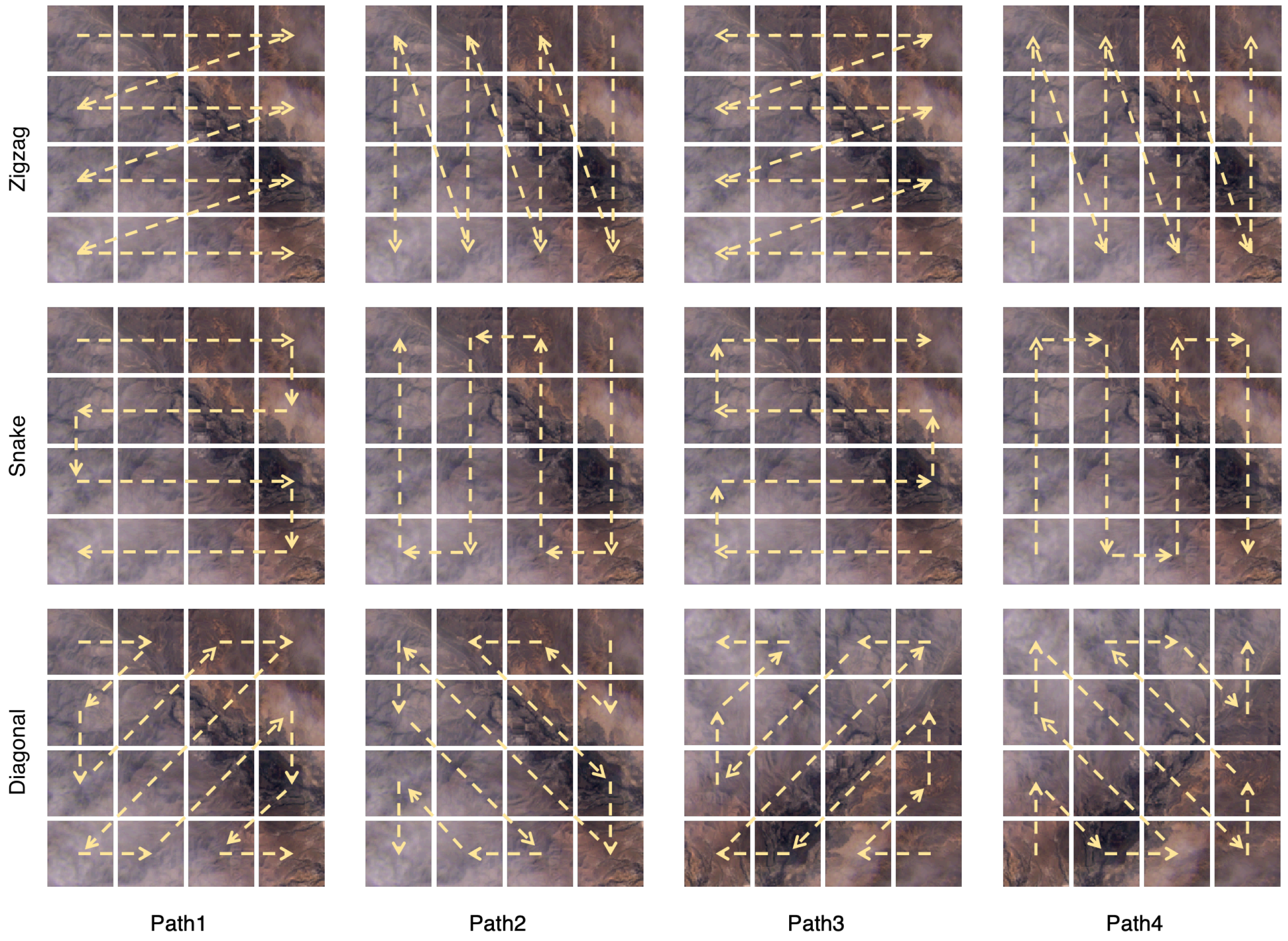
The MPS2D module employs three distinct scanning patterns: Zigzag, Snake, and Diagonal trajectories (Figure 3). The Zigzag pattern scans sequentially along the horizontal axisl the Snake pattern interleaves horizontal and vertical movements; and the Diagonal pattern captures spatial relationships across diagonal directions. Specifically, the Zigzag pattern sequentially scans the image from left to right in each row and then moves downward to the next row. The Snake pattern, which is similar to the zigzag pattern but smoother, follows a continuous winding motion. The Diagonal pattern scans diagonally across the image, linking patches in the row and column directions simultaneously and emphasizing cross-directional dependencies over strictly horizontal or vertical movements. All scanning patterns in MPSM are implemented in a pixel-by-pixel manner to preserve spatial continuity and avoid border discontinuities introduced by patch-based division.

3.3.2. ScanPattern Module

In MPS2D, all scanning patterns feature four corner-initiated traversal paths (top-left, top-right, bottom-right, bottom-left) (Figure 3). The detailed architecture of the ScanPattern module is presented in Figure 2d. Given an input X , the ScanPattern module can be formally expressed in Equation (8):
ScanPattern ( X ) = [ X 1 , X 2 , X 3 , X 4 ] ,
where X 1 , X 2 , X 3 , X 4 can be formulated as in Equation (9)):
X 1 = S 6 ( Path 1 ( X ) ) , X 2 = S 6 ( Path 2 ( X ) ) , X 3 = S 6 ( Path 3 ( X ) ) , X 4 = S 6 ( Path 4 ( X ) ) ,
where S6 denotes the fundamental processing module in vanilla Mamba [24].

3.3.3. Dynamic Path-Aware Module

The DPA module aims to fuse features from multiple paths by recalibrating feature contributions at spatial locations. In detail, for each component of the feature embedding, k feature values are generated through k different traversal paths. We introduce the coefficient of variation (CV) as a metric to measure the dispersion of these k feature values.
If the k feature values are highly consistent (small CV), these features are insensitive to the traversal paths and may be irrelevant; conversely, if the k feature values exhibit significant variation (large CV), these features are sensitive to the traversal paths and likely contain important positional information, making them worth preserving or further enhancing. The coefficient of variation is defined as follows:
x cv = std ( [ x j ] ) / avg ( [ x j min ( [ x j ] ) ] ) ,
where x j represents the value from the j-th traversal path, with j ranging from 1 to k. Figure 2e illustrates the structure of the DPA module, which consists of two branches. One performs feature summation along the path dimension, while the other computes CV and then implements a ReLU function to generate position-specific weight guidance. The outputs of both branches are then fused via element-wise multiplication. Given four inputs X 1 , X 2 , X 3 , X 4 , the DPA module is expressed in Equation (11):
Y = ReLU ( CV ( X 1 , X 2 , X 3 , X 4 ) ) Sum ( X 1 , X 2 , X 3 , X 4 ) ,
where CV computes the coefficient of variation, ⊗ is the Hadamard product, and Sum aggregates the feature maps along the channel dimension.
The pseudo-code for the MPS2D module is presented in Algorithm 1. This algorithm provides a detailed step-by-step representation of the module’s operational logic.
Algorithm 1 Pseudo-Code for Multi-Pattern Scanning 2D (MPS2D) module
Input: X i n , a feature map of shape [ B , H , W , C ] (batch size, height, width, channel); m, number of heads; k, number of traversal paths.
Output: X o u t , result of MPS2D module with shape [ B , H , W , C ] .
   
# Reshape the input feature map, shape = [ B , C , H , W ]
1:
X Reshape ( X i n )
   
# Process with m scanning patterns
2:
for  i = 1  to  m  do
3:
    X i Pattern i ( X )
   
# Process with k traversal paths
4:
   for  j = 1  to k do
5:
      X i j Path j ( X i )
6:
      X i j S 6 ( X i j )
7:
      X i j ReArrange ( X i j )
8:
   end for
9:
    Y i Concat ( X i 1 , X i 2 , , X i k )
10:
    Y c v CoefficientVariation ( Y i )
11:
    Y i ReLU ( Y c v ) Sum ( Y i )
12:
end for
   
# Concatenate along the channel axis
13:
Y Concat ( Y 1 , Y 2 , , Y m )
14:
Y LayerNorm ( Y )
   
# Reshape the feature map to original dimensions, shape = [ B , H , W , C ]
15:
X o u t Reshape ( Y )

4. Results

4.1. Experimental Setting

4.1.1. Datasets

We evaluate our method on four benchmark datasets: RICE1 [51], RICE2 [51], T-CLOUD [11], and SEN12MS-CR [52]. Table 2 presents the main properties of each dataset. RICE1 [51] is collected from Google Earth by toggling the display of the cloud layer. It consists of 500 non-overlapping cloudy–cloudless image pairs, which are split into 400 pairs for training and 100 pairs for testing. RICE2 [51], derived from the Landsat 8 OLI/TIRS, presents more challenging cloud conditions characterized by thick and complex cloud coverage. It consists of 735 cloudy–cloudless image pairs, divided into 588 pairs for training and 147 pairs for testing. T-CLOUD [11] is derived from Landsat 8 RGB images. It comprises 2939 cloudy–cloudless pairs, split into 2351 pairs for training and 588 pairs for testing. SEN12MS-CR [52] is a large-scale multi-spectral dataset covering 175 regions worldwide across four seasons. It provides co-registered Sentinel-1 SAR and Sentinel-2 optical image pairs for cloud-removal tasks. Each sample consists of a triplet of radar and optical observations with and without cloud cover. The dataset contains a total of 122,218 pairs of 256 × 256 pixels, including 114,325 for training and 7893 for testing.

4.1.2. Evaluation Metrics

We follow previous cloud-removal algorithms [15,17,26] with four evaluation metrics including mean absolute error (MAE) [53], peak signal-to-noise ratio (PSNR) [54], structural similarity index (SSIM) [55], and spectral angle mapper (SAM) [56].

4.1.3. Implementation Details

The proposed method is implemented using the PyTorch 2.1.1 framework and trained utilizing one NVIDIA RTX 3090 GPU. We adopt the Adam optimizer with β 1 = 0.9 and β 2 = 0.999. The initial learning rate is set to 0.0005 and is progressively reduced to 1 × 10 6 via a cosine annealing strategy [57]. The training patches are dimensioned at 256 × 256 pixels. The model undergoes training for 1000 epochs with a batch size of 16 to ensure comprehensive learning and convergence.

4.2. Comparison with State-of-the-Art Methods

We evaluate the superiority of our method through quantitative and qualitative comparisons with several representative cloud-removal models, including CNN-based methods (pix2pix [7], SPA-GAN [26], RCA-Net [25]), Transformer-based methods (CVAE [11], Restormer [19], Trinity-Net [16], CMNet [17], CR-Former [20]), and a recent Mamba-based method (CR-Famba [42]).
RICE1: Table 3 shows that our method achieves the lowest MAE (0.014) and SAM (0.92) while attaining the highest PSNR (36.65) and SSIM (0.9625).
Our approach significantly surpasses the performance of earlier models such as Pix2Pix [7], SPA-GAN [26], and RCA-Net [25]. Furthermore, when evaluated against recent methods, including CMNet [17] and CR-Former [20], our method consistently achieves superior performance metrics. Similarly, our approach substantially outperforms recent state-space model-based CR-Famba [42]. In addition, our approach exhibits remarkable computational efficiency. It requires only 4.27 M parameters and 32.6 G FLOPs, significantly fewer than Restormer [19] (26.13 M, 155.0 G), CMNet [17] (16.51 M, 236.0 G), and CR-Famba [42] (174.94 M, 165.0 G). Compared to other methods, ours delivers the best accuracy and requires a relatively low computational overhead. These results indicate that our method achieves balance between accuracy and computational efficiency on the RICE1 dataset.
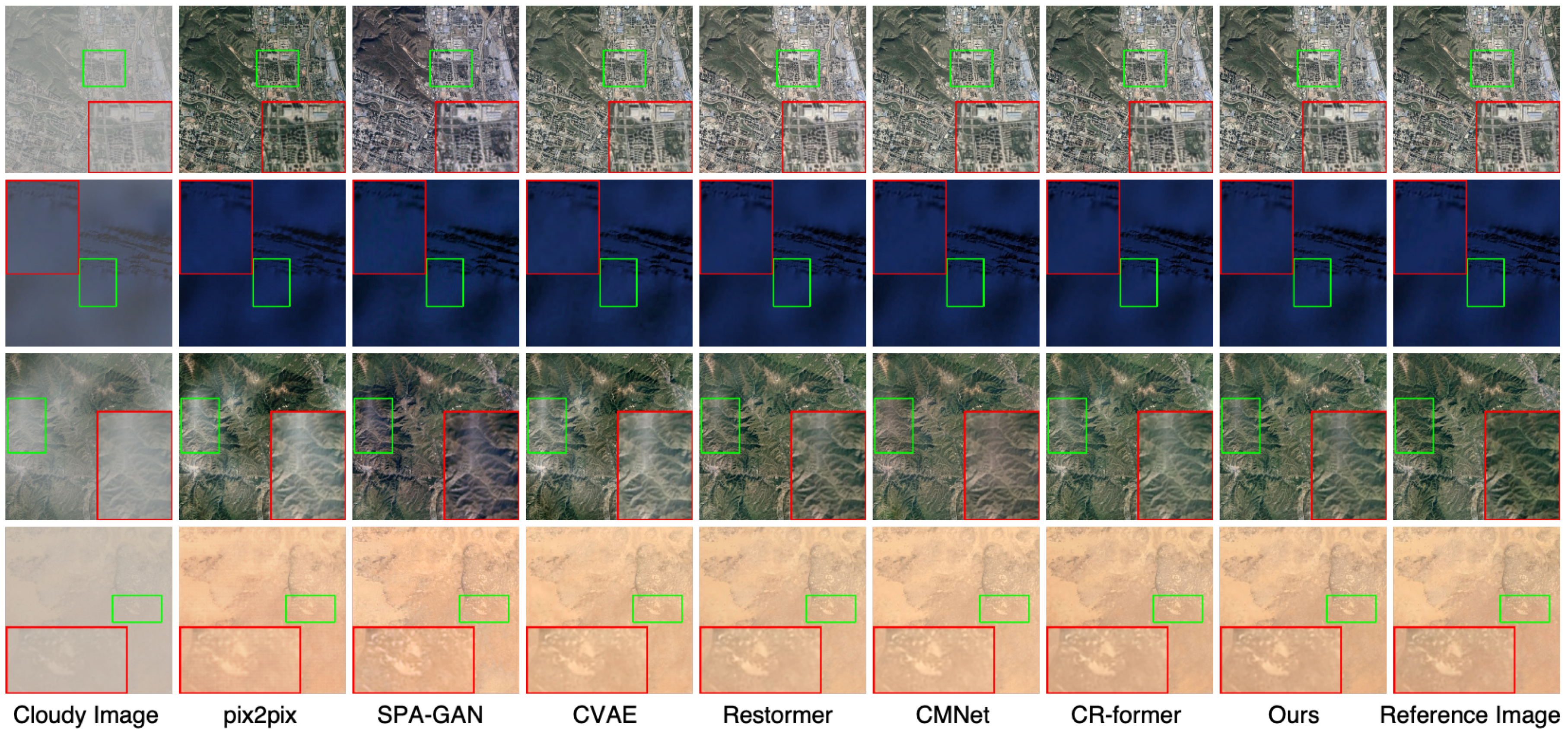
Figure 4 illustrates that our method significantly outperforms other approaches. With pix2pix [7], SPA-GAN [26], CVAE [11], and Restormer [19], residual cloud artifacts remain visible in localized areas, while with our method, large cloud-covered regions are almost completely removed. Furthermore, while CMNet [17] and CR-former [20]—two recently published approaches—exhibit strong cloud-removal capabilities in large occluded regions, as our method does, our method shows a more refined removal of residual cloud textures in small-scale regions, indicating that our multi-scale framework effectively enhances fine-detail restoration.
RICE2: Table 4 shows that our approach continues to lead in performance. Despite the increased complexity of this dataset, our method maintains the lowest MAE (0.0156) and SAM (1.21) while achieving the highest PSNR (36.38) and SSIM (0.9168), confirming its ability to produce high-quality reconstructions even in more difficult scenarios. Compared to the second-best CR-former [20], our method reduces MAE by 0.0005 and SAM by 0.07 while improving PSNR by 0.17 and SSIM by 0.0017. In addition, our method retains its advantage in computational efficiency, with minimal parameter and FLOP usage. Compared to recent approaches such as CMNet [17], CR-former [20] and CR-Famba [42], our method significantly reduces computational overhead. These findings demonstrate that our method not only excels in standard conditions but also remains highly robust on the more challenging RICE2 dataset.
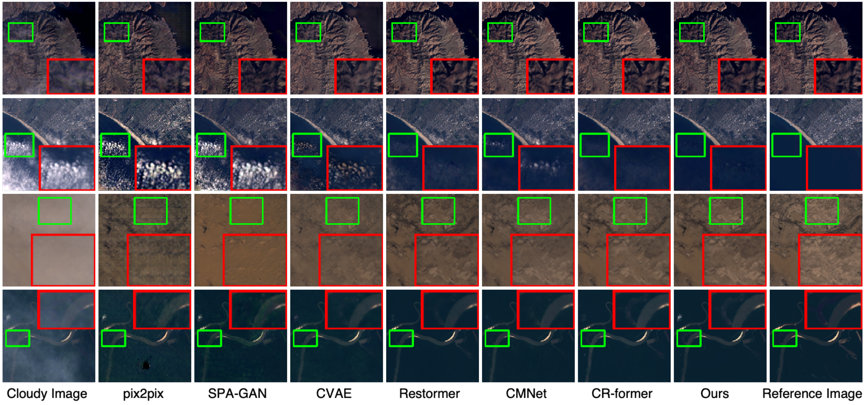
Figure 5 presents the results on four images with different cloud characteristics, arranged sequentially. It shows that our method consistently achieves superior performance across different types of cloud cover, confirming its robustness. In cases of thin cloud layers, most methods perform well in removing large cloud-covered areas; however, our approach demonstrates superior detail recovery for fine structures. In scenarios with denser cloud covers, the advantage of our method becomes even more evident.
T-CLOUD: Table 5 shows that our method achieves the lowest MAE (0.0237) and SAM (2.36) while attaining the highest PSNR (30.82) and SSIM (0.8887), indicating its effectiveness in reducing reconstruction errors and preserving structural details in highly complex settings. In addition, our method maintains its computational efficiency. Compared to CR-former [20], an efficient vision transformer variant that balances model size and accuracy, our method reduces Params by 12.91 M and FLOPs by 28.29 G. Moreover, our method substantially outperforms the recent state space model-based CR-Famba [42] in overhead. These findings further demonstrate the robustness and strong generalization ability of our method on diverse datasets.
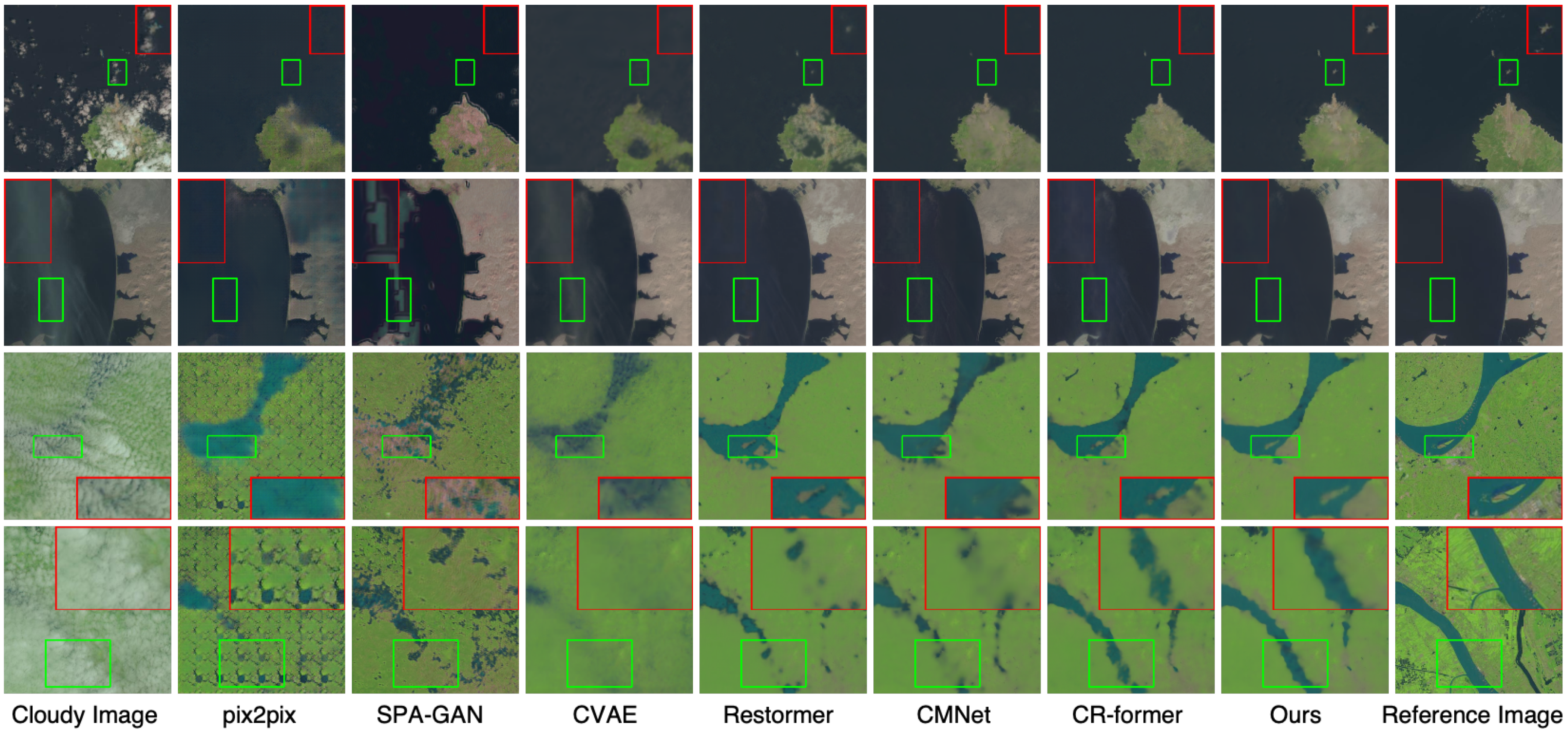
As shown in Figure 6, the outputs of our method are visually closest to the reference images. Our approach markedly outperforms pix2pix [7], SPA-GAN [26], and CVAE [11], especially on the fourth image. In our technique, extensive cloud-covered areas are nearly fully cleared, whereas the other methods leave noticeable cloud remnants in localized regions. Furthermore, compared to CMNet [17] and CR-former [20]—two of the latest state-of-the-art methods—our method delivers a more polished elimination of residual cloud textures in finer details, suggesting that our framework excels in enhancing precise restoration.

4.3. Evaluation on the Multi-Modal SEN12MS-CR Dataset

To further verify the generalization ability of the proposed model in multi-modal scenarios, we conducted experiments on the large-scale SEN12MS-CR dataset [52], which contains triplets of SAR images, cloudy optical images, and corresponding cloud-free optical images. In this experiment, the SAR data are treated as an additional input channel concatenated with the optical images and the proposed model was directly applied without introducing any specialized multi-modal fusion modules. As shown in Table 6, the proposed method achieves superior performance compared with several representative SAR-assisted cloud-removal approaches, including DSen2-CR [58], GLF-CR [15], and UnCRtainTS [59]. Specifically, our model attains the best performance in terms of MAE (0.026), SAM (8.220), PSNR (29.59), and SSIM (0.893), demonstrating its strong potential for use in broader multi-modal remote sensing restoration tasks.

5. Discussion

This section presents comprehensive ablation experiments to validate the effectiveness and robustness of our framework. We first analyze the impact of key architectural components, then evaluate its robustness under different cloud conditions and ground backgrounds, and finally examine the model’s efficiency and scalability.

5.1. Architecture-Level Ablations

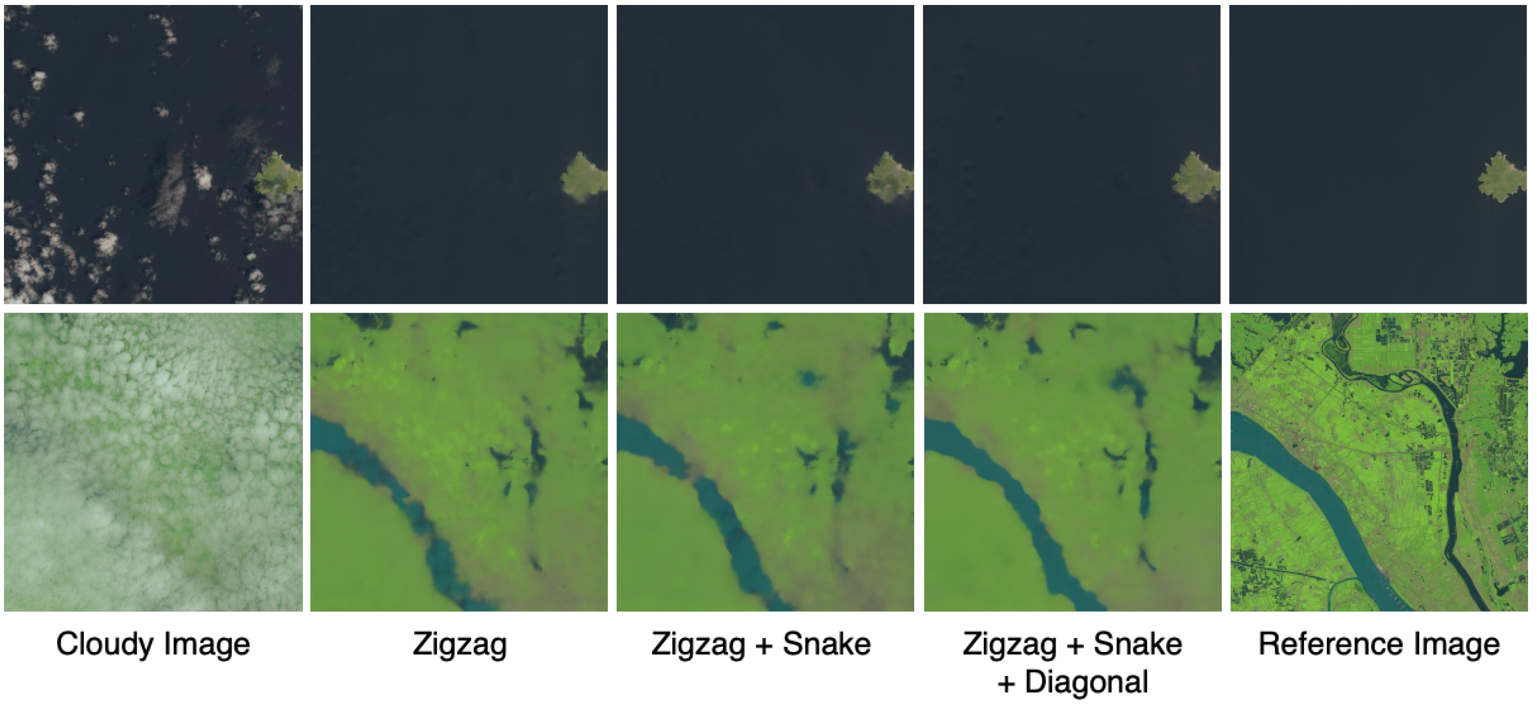
Effects of Multiple Scanning Patterns: The results in Table 7 show that the use of a single scanning pattern alone yields limited performance, indicating that each individual strategy (Zigzag, Snake, and Diagonal) captures only partial spatial dependencies. When two patterns are combined, moderate improvements can be observed in some cases. For example, the combination Zigzag + Snake enhances all four metrics compared with either pattern alone, while Zigzag + Diagonal slightly improves PSNR and Snake + Diagonal results in a minor gain in MAE. By contrast, integrating all three patterns (Zigzag + Snake + Diagonal) yields the best overall results, demonstrating that the joint use of complementary scanning paths effectively improves spatial context modeling without increasing computational overhead.
The qualitative results in Figure 7 also illustrate that the progressive incorporation of scanning patterns enhances the clarity of recovered ground objects. This indicates that the combined use of diverse scanning strategies improves long-range dependency modeling on 2D cloudy images. Meanwhile, this improvement is accompanied by a reduction in computational overhead (Table 7), with Params decreasing from 4.38 M to 4.27 M and FLOPs dropping from 33.45 G to 32.6 G. These findings indicate that the joint use of diverse scanning strategies not only alleviates the limitation of a single scanning pattern, but also keeps computational complexity relatively low.
Block-Level Comparison: To isolate the contribution of the proposed MPSM block, we compare U-Net (vanilla Mamba) and U-Net (MPSM) under identical settings. As shown in Table 8, U-Net (MPSM, full version) demonstrates consistent advantages over U-Net (vanilla Mamba), with reductions of 0.0006 in MAE and 0.07 in SAM and improvements of 0.51 in PSNR and 0.009 in SSIM, confirming that the performance improvements originate from the proposed MPSM design rather than from the U-Net backbone itself.
Analysis of the Dynamic Path-Aware Mechanism:The dynamic path-aware (DPA) mechanism, a key component of the dynamic path-aware module, enhances the implicit perception of positional information in the model by dynamically adjusting feature importance based on the dispersion of features across different scanning paths. Table 8 shows that the baseline (without DPA) yields an MAE of 0.0157, an SAM of 1.25, a PSNR of 36.07, and an SSIM of 0.9175. When DPA is incorporated with our method, the metrics are reduced to an MAE of 0.0156 and an SAM of 1.21, with the PSNR improving to 36.38 and Params and FLOPs maintained at 4.27 M at 32.6 G, respectively. This set of results indicates that DPA effectively enhances spatial awareness by focusing on position-sensitive features. Moreover, this mechanism does not increase the computational complexity of the model.
Effects of the Multi-Scale Loss:Table 8 shows that the multi-scale supervision loss further refines the model’s performance by applying independent loss constraints at different resolution levels, enabling better capture of cloud structures across multiple feature hierarchies. Compared to the configuration without L M S (MAE of 0.0159, SAM of 1.24, PSNR of 36.25, SSIM of 0.9159), our model, with the inclusion of L M S , achieves a reduced MAE of 0.0156, a lower SAM of 1.21, and improved PSNR and SSIM values (36.38 and 0.9168, respectively), with a slight increase in parameters (from 4.26 M to 4.27 M) and FLOPs (from 32.53 G to 32.6 G). This shows that L M S facilitates the joint learning of fine-grained local characteristics and global representations with relatively low computational cost.

5.2. Comparison Under Varying Cloud and Surface Conditions

To further assess the robustness of our method, we qualitatively evaluated its restoration performance under different cloud conditions. As shown in Figure 8, the first two columns correspond to thin and semi-transparent clouds, a condition under which our model achieves nearly seamless restoration, with well-preserved surface details. The middle two columns represent locally dense cloud coverage, a condition under which the model effectively removes the clouds and restores the overall structure and contours, with slight blurring observed in some local texture details. The last two columns show large-scale distributed thick clouds, with most of the ground surface heavily obscured. Although the model’s fine-grained recovery is less precise under conditions of such dense coverage compared to thin-cloud cases, it still reconstructs visually reasonable structures and colors, maintaining overall consistency.
Figure 8 illustrates that our method shows generally stable restoration performance across various land-cover backgrounds under similar cloud conditions. Under conditions of thin or semi-transparent clouds (urban, mountainous), the restored edges and textures remain clear, with consistent color tone across different surfaces. Under conditions of locally dense cloud coverage (urban, vegetation, river), the model maintains coherent global structure and balanced color distribution, with only minor variations in texture smoothness among backgrounds. For thick distributed clouds (urban, mountainous), the model still produces plausible structures and colors across different terrains, without noticeable degradation in any specific background. Overall, the differences in restoration quality across various land surfaces are relatively small, suggesting that the proposed framework generalizes well to diverse ground conditions.

5.3. Efficiency and Scalability

To provide a more realistic evaluation of computational efficiency, we report practical metrics that include the average inference time per image and GPU memory consumption, as summarized in Table 9. All experiments were conducted on an NVIDIA RTX 3090 GPU with an input resolution of 256 × 256. The results show that our proposed model achieves a favorable balance between accuracy and efficiency, requiring only 4.27 M parameters and 32.6 G FLOPs while maintaining an average inference time of 75.78 ms and the lowest GPU memory usage (1094 MB) among all competitors. Compared with recent Transformer-based and Mamba-based models, our method demonstrates significantly lower computational cost and better deployment potential on real hardware devices without sacrificing restoration performance.
Table 10 presents the quantitative results of the scalability analysis under different image resolutions. The model is trained on 256 × 256 pixels and tested across various resolutions ranging from 32 × 32 pixels to 2048 × 2048 pixels. The results show that our method maintains stable performance across scales, with the best quantitative results in MAE, SAM, and PSNR at a resolution of 384 × 384 pixels. When the resolution increases beyond 1024 × 1024 pixels, SSIM continues to improve, while other metrics slightly decrease. This is because SSIM focuses on local structural consistency rather than pixel-wise accuracy. When the resolution drops below 256 × 256 pixels, the performance decreases notably in terms of PSNR and SSIM. This degradation is mainly due to the severe loss of fine spatial and spectral details after downsampling. Overall, the model demonstrates better restoration quality when tested on images with resolutions higher than those in the training scale, compared with its performance on lower-resolution images. In terms of computational efficiency, the increase in FLOPs, inference time, and GPU memory usage with higher input resolutions is an expected outcome, as the number of processed pixels grows quadratically with image size. Nevertheless, our model shows favorable scalability: when the resolution increases from 256 × 256 to 1024 × 1024 (a 16-fold increase in pixel count), the inference time rises to 1128.41 ms (a 14.9-fold increase), which remains below the theoretical linear growth.

6. Conclusions

This paper proposes a multi-pattern scanning Mamba framework tailored for cloud removal. Specifically, we design a multi-pattern scanning Mamba (MPSM) block that employs three sequential patterns (Zigzag, Snake, and Diagonal) to capture long-range spatial correlations. Within the MPSM block, each pattern is further enhanced with four traversal paths to aggregate contextual information across the entire feature map. Moreover, we design a dynamic path-aware (DPA) mechanism to adaptively recalibrate the feature contributions from multi-directional paths. Finally, we construct a U-Net-style architecture centered on the MPSM block and incorporate a multi-scale supervision loss to jointly optimize local details and global structures. Experimental results on three popular remote sensing datasets show that our framework outperforms existing state-of-the-art methods while maintaining a relatively low computational cost.

Author Contributions

Conceptualization, X.X., Y.D. and W.H.; Data curation, W.H.; Formal analysis, X.X., Y.D. and W.H.; Funding acquisition, J.W.; Investigation, Y.D. and W.H.; Methodology, X.X. and Y.D.; Software, W.H. and Y.W.; Supervision, J.W.; Validation, Y.D. and W.H.; Visualization, X.X.; Writing—original draft, X.X.; Writing—review & editing, Y.D., W.H., Y.W. and J.F. All authors have read and agreed to the published version of the manuscript.

Funding

This work was supported in part by the National Key Research and Development Project under Grant 2024YFB4708100, National Natural Science Foundation of China under Grants U24A20325 and 12326608, and in part by the Sichuan Science Foundation project under Grant 2024ZDZX0002 and 2024NSFTD0054, the Public Welfare Research Program of Ningbo City under Grant 2024S063.

Data Availability Statement

The code will be available at https://github.com/xmengxin/MPS-Mamba, accessed on 26 October 2025.

Conflicts of Interest

Author Jie Fang was employed by the company Hangzhou Halome Cloud Technology Company Limited. The remaining authors declare that the research was conducted in the absence of any commercial or financial relationships that could be construed as a potential conflict of interest.

References

  1. Azimi, S.M.; Vig, E.; Bahmanyar, R.; Körner, M.; Reinartz, P. Towards multi-class object detection in unconstrained remote sensing imagery. In Proceedings of the Asian Conference on Computer Vision, Perth, Australia, 2–6 December 2018; Springer: Berlin/Heidelberg, Germany, 2018; pp. 150–165. [Google Scholar]
  2. Wang, P.; Sun, X.; Diao, W.; Fu, K. FMSSD: Feature-merged single-shot detection for multiscale objects in large-scale remote sensing imagery. IEEE Trans. Geosci. Remote Sens. 2019, 58, 3377–3390. [Google Scholar] [CrossRef]
  3. Carranza-García, M.; García-Gutiérrez, J.; Riquelme, J.C. A framework for evaluating land use and land cover classification using convolutional neural networks. Remote Sens. 2019, 11, 274. [Google Scholar] [CrossRef]
  4. Tong, X.Y.; Xia, G.S.; Lu, Q.; Shen, H.; Li, S.; You, S.; Zhang, L. Land-cover classification with high-resolution remote sensing images using transferable deep models. Remote Sens. Environ. 2020, 237, 111322. [Google Scholar] [CrossRef]
  5. Stumpf, F.; Schneider, M.K.; Keller, A.; Mayr, A.; Rentschler, T.; Meuli, R.G.; Schaepman, M.; Liebisch, F. Spatial monitoring of grassland management using multi-temporal satellite imagery. Ecol. Indic. 2020, 113, 106201. [Google Scholar] [CrossRef]
  6. Wang, Y.; Zhang, B.; Zhang, W.; Hong, D.; Zhao, B.; Li, Z. Cloud removal with SAR-optical data fusion using a unified spatial–spectral residual network. IEEE Trans. Geosci. Remote Sens. 2023, 62, 5600820. [Google Scholar] [CrossRef]
  7. Isola, P.; Zhu, J.Y.; Zhou, T.; Efros, A.A. Image-to-image translation with conditional adversarial networks. In Proceedings of the IEEE Conference on Computer Vision and Pattern Recognition, Honolulu, HI, USA, 21–26 July 2017; pp. 1125–1134. [Google Scholar]
  8. Malek, S.; Melgani, F.; Bazi, Y.; Alajlan, N. Reconstructing cloud-contaminated multispectral images with contextualized autoencoder neural networks. IEEE Trans. Geosci. Remote Sens. 2017, 56, 2270–2282. [Google Scholar] [CrossRef]
  9. Li, W.; Li, Y.; Chen, D.; Chan, J.C.W. Thin cloud removal with residual symmetrical concatenation network. ISPRS J. Photogramm. Remote Sens. 2019, 153, 137–150. [Google Scholar] [CrossRef]
  10. Yu, W.; Zhang, X.; Pun, M.O. Cloud removal in optical remote sensing imagery using multiscale distortion-aware networks. IEEE Geosci. Remote Sens. Lett. 2022, 19, 5512605. [Google Scholar] [CrossRef]
  11. Ding, H.; Zi, Y.; Xie, F. Uncertainty-based thin cloud-removal network via conditional variational autoencoders. In Proceedings of the Asian Conference on Computer Vision, Macao, China, 4–8 December 2022; pp. 469–485. [Google Scholar]
  12. Wu, P.; Pan, Z.; Tang, H.; Hu, Y. Cloudformer: A cloud-removal network combining self-attention mechanism and convolution. Remote Sens. 2022, 14, 6132. [Google Scholar] [CrossRef]
  13. Zhao, B.; Zhou, J.; Xu, H.; Feng, X.; Sun, Y. PM-LSMN: A Physical-Model-based Lightweight Self-attention Multiscale Net For Thin Cloud Removal. IEEE Geosci. Remote Sens. Lett. 2024, 21, 5003405. [Google Scholar] [CrossRef]
  14. Vaswani, A.; Shazeer, N.; Parmar, N.; Uszkoreit, J.; Jones, L.; Gomez, A.N.; Kaiser, Ł.; Polosukhin, I. Attention is all you need. Adv. Neural Inf. Process. Syst. 2017, 30, 5998–6008. [Google Scholar]
  15. Xu, F.; Shi, Y.; Ebel, P.; Yu, L.; Xia, G.S.; Yang, W.; Zhu, X.X. GLF-CR: SAR-enhanced cloud removal with global–local fusion. ISPRS J. Photogramm. Remote Sens. 2022, 192, 268–278. [Google Scholar] [CrossRef]
  16. Chi, K.; Yuan, Y.; Wang, Q. Trinity-Net: Gradient-guided Swin transformer-based remote sensing image dehazing and beyond. IEEE Trans. Geosci. Remote Sens. 2023, 61, 4702914. [Google Scholar] [CrossRef]
  17. Liu, J.; Pan, B.; Shi, Z. Cascaded Memory Network for Optical Remote Sensing Imagery Cloud Removal. IEEE Trans. Geosci. Remote Sens. 2024, 62, 5613611. [Google Scholar] [CrossRef]
  18. Liu, Z.; Lin, Y.; Cao, Y.; Hu, H.; Wei, Y.; Zhang, Z.; Lin, S.; Guo, B. Swin transformer: Hierarchical vision transformer using shifted windows. In Proceedings of the IEEE/CVF International Conference on Computer Vision, Online, 11–17 October 2021; pp. 10012–10022. [Google Scholar]
  19. Zamir, S.W.; Arora, A.; Khan, S.; Hayat, M.; Khan, F.S.; Yang, M.H. Restormer: Efficient transformer for high-resolution image restoration. In Proceedings of the IEEE/CVF Conference on Computer Vision and Pattern Recognition, New Orleans, LA, USA, 18–24 June 2022; pp. 5728–5739. [Google Scholar]
  20. Wu, Y.; Deng, Y.; Zhou, S.; Liu, Y.; Huang, W.; Wang, J. CR-former: Single Image Cloud Removal with Focused Taylor Attention. IEEE Trans. Geosci. Remote Sens. 2024, 62, 5651614. [Google Scholar] [CrossRef]
  21. Gu, A.; Goel, K.; Ré, C. Efficiently modeling long sequences with structured state spaces. arXiv 2021, arXiv:2111.00396. [Google Scholar]
  22. Gu, A.; Johnson, I.; Goel, K.; Saab, K.; Dao, T.; Rudra, A.; Ré, C. Combining recurrent, convolutional, and continuous-time models with linear state space layers. Adv. Neural Inf. Process. Syst. 2021, 34, 572–585. [Google Scholar]
  23. Smith, J.T.; Warrington, A.; Linderman, S.W. Simplified state space layers for sequence modeling. arXiv 2022, arXiv:2208.04933. [Google Scholar]
  24. Gu, A.; Dao, T. Mamba: Linear-time sequence modeling with selective state spaces. arXiv 2023, arXiv:2312.00752. [Google Scholar] [CrossRef]
  25. Wen, X.; Pan, Z.; Hu, Y.; Liu, J. An Effective Network Integrating Residual Learning and Channel Attention Mechanism for Thin Cloud Removal. IEEE Geosci. Remote. Sens. Lett. 2022, 19, 6507605. [Google Scholar] [CrossRef]
  26. Pan, H. Cloud removal for remote sensing imagery via spatial attention generative adversarial network. arXiv 2020, arXiv:2009.13015. [Google Scholar] [CrossRef]
  27. Singh, P.; Komodakis, N. Cloud-gan: Cloud removal for sentinel-2 imagery using a cyclic consistent generative adversarial networks. In Proceedings of the IGARSS 2018—2018 IEEE International Geoscience and Remote Sensing Symposium, Valencia, Spain, 22–27 July 2018; pp. 1772–1775. [Google Scholar]
  28. Zhu, J.Y.; Park, T.; Isola, P.; Efros, A.A. Unpaired image-to-image translation using cycle-consistent adversarial networks. In Proceedings of the IEEE International Conference on Computer Vision, Venice, Italy, 22–29 October 2017; pp. 2223–2232. [Google Scholar]
  29. Ma, X.; Huang, Y.; Zhang, X.; Pun, M.O.; Huang, B. Cloud-egan: Rethinking cyclegan from a feature enhancement perspective for cloud removal by combining cnn and transformer. IEEE J. Sel. Top. Appl. Earth Obs. Remote Sens. 2023, 16, 4999–5012. [Google Scholar] [CrossRef]
  30. Mao, R.; Li, H.; Ren, G.; Yin, Z. Cloud removal based on SAR-optical remote sensing data fusion via a two-flow network. IEEE J. Sel. Top. Appl. Earth Obs. Remote Sens. 2022, 15, 7677–7686. [Google Scholar] [CrossRef]
  31. Anandakrishnan, J.; Sundaram, V.M.; Paneer, P. CERMF-Net: A SAR-Optical feature fusion for cloud elimination from Sentinel-2 imagery using residual multiscale dilated network. IEEE J. Sel. Top. Appl. Earth Obs. Remote Sens. 2024, 17, 11741–11749. [Google Scholar] [CrossRef]
  32. Wen, X.; Pan, Z.; Hu, Y.; Liu, J. Generative adversarial learning in YUV color space for thin cloud removal on satellite imagery. Remote Sens. 2021, 13, 1079. [Google Scholar] [CrossRef]
  33. Chen, Z.; Zhang, Y.; Gu, J.; Kong, L.; Yang, X.; Yu, F. Dual aggregation transformer for image super-resolution. In Proceedings of the IEEE/CVF International Conference on Computer Vision, Paris, France, 2–6 October 2023; pp. 12312–12321. [Google Scholar]
  34. Li, Y.; Fan, Y.; Xiang, X.; Demandolx, D.; Ranjan, R.; Timofte, R.; Van Gool, L. Efficient and explicit modelling of image hierarchies for image restoration. In Proceedings of the IEEE/CVF Conference on Computer Vision and Pattern Recognition, Paris, France, 2–6 October 2023; pp. 18278–18289. [Google Scholar]
  35. Xu, M.; Deng, F.; Jia, S.; Jia, X.; Plaza, A.J. Attention mechanism-based generative adversarial networks for cloud removal in Landsat images. Remote Sens. Environ. 2022, 271, 112902. [Google Scholar] [CrossRef]
  36. Liu, H.; Huang, J.; Nie, J.; Xie, J.; Chen, L.; Zhou, X. Density Guided and Frequency Modulation Dehazing Network for Remote Sensing Images. IEEE J. Sel. Top. Appl. Earth Obs. Remote Sens. 2025, 18, 9533–9545. [Google Scholar] [CrossRef]
  37. Mehta, H.; Gupta, A.; Cutkosky, A.; Neyshabur, B. Long range language modeling via gated state spaces. arXiv 2022, arXiv:2206.13947. [Google Scholar] [CrossRef]
  38. Fu, D.Y.; Dao, T.; Saab, K.K.; Thomas, A.W.; Rudra, A.; Ré, C. Hungry hungry hippos: Towards language modeling with state space models. arXiv 2022, arXiv:2212.14052. [Google Scholar]
  39. Liu, Y.; Tian, Y.; Zhao, Y.; Yu, H.; Xie, L.; Wang, Y.; Ye, Q.; Jiao, J.; Liu, Y. Vmamba: Visual state space model. Adv. Neural Inf. Process. Syst. 2024, 37, 103031–103063. [Google Scholar]
  40. Guo, H.; Li, J.; Dai, T.; Ouyang, Z.; Ren, X.; Xia, S.T. Mambair: A simple baseline for image restoration with state-space model. In Proceedings of the European Conference on Computer Vision, Milan, Italy, 29 September–4 October 2024; Springer: Berlin/Heidelberg, Germany, 2024; pp. 222–241. [Google Scholar]
  41. Zhang, C.; Wang, F.; Zhang, X.; Wang, M.; Wu, X.; Dang, S. Mamba-CR: A state-space model for remote sensing image cloud removal. IEEE Trans. Geosci. Remote Sens. 2024, 63, 5601913. [Google Scholar] [CrossRef]
  42. Liu, J.; Pan, B.; Shi, Z. CR-Famba: A frequency-domain assisted mamba for thin cloud removal in optical remote sensing imagery. IEEE Trans. Multimed. 2025, 27, 5659–5668. [Google Scholar] [CrossRef]
  43. Martin, E.; Cundy, C. Parallelizing linear recurrent neural nets over sequence length. arXiv 2017, arXiv:1709.04057. [Google Scholar]
  44. Wang, J.; Zhu, W.; Wang, P.; Yu, X.; Liu, L.; Omar, M.; Hamid, R. Selective structured state-spaces for long-form video understanding. In Proceedings of the IEEE/CVF Conference on Computer Vision and Pattern Recognition, Vancouver, BC, Canada, 17–24 June 2023; pp. 6387–6397. [Google Scholar]
  45. Li, K.; Li, X.; Wang, Y.; He, Y.; Wang, Y.; Wang, L.; Qiao, Y. Videomamba: State space model for efficient video understanding. In Proceedings of the European Conference on Computer Vision, Milan, Italy, 29 September–4 October 2024; Springer: Berlin/Heidelberg, Germany, 2024; pp. 237–255. [Google Scholar]
  46. Ma, J.; Li, F.; Wang, B. U-mamba: Enhancing long-range dependency for biomedical image segmentation. arXiv 2024, arXiv:2401.04722. [Google Scholar]
  47. Islam, M.M.; Hasan, M.; Athrey, K.S.; Braskich, T.; Bertasius, G. Efficient movie scene detection using state-space transformers. In Proceedings of the IEEE/CVF Conference on Computer Vision and Pattern Recognition, Vancouver, BC, Canada, 17–24 June 2023; pp. 18749–18758. [Google Scholar]
  48. Nguyen, E.; Goel, K.; Gu, A.; Downs, G.; Shah, P.; Dao, T.; Baccus, S.; Ré, C. S4nd: Modeling images and videos as multidimensional signals with state spaces. Adv. Neural Inf. Process. Syst. 2022, 35, 2846–2861. [Google Scholar]
  49. Qiao, Y.; Yu, Z.; Guo, L.; Chen, S.; Zhao, Z.; Sun, M.; Wu, Q.; Liu, J. Vl-mamba: Exploring state space models for multimodal learning. arXiv 2024, arXiv:2403.13600. [Google Scholar] [CrossRef]
  50. Ronneberger, O.; Fischer, P.; Brox, T. U-net: Convolutional networks for biomedical image segmentation. In Proceedings of the Medical Image Computing and Computer-Assisted Intervention—MICCAI 2015: 18th International Conference, Munich, Germany, 5–9 October 2015; Springer: Berlin/Heidelberg, Germany, 2015. Proceedings, Part III 18. pp. 234–241. [Google Scholar]
  51. Lin, D.; Xu, G.; Wang, X.; Wang, Y.; Sun, X.; Fu, K. A remote sensing image dataset for cloud removal. arXiv 2019, arXiv:1901.00600. [Google Scholar] [CrossRef]
  52. Ebel, P.; Meraner, A.; Schmitt, M.; Zhu, X.X. Multisensor data fusion for cloud removal in global and all-season sentinel-2 imagery. IEEE Trans. Geosci. Remote Sens. 2020, 59, 5866–5878. [Google Scholar] [CrossRef]
  53. Chai, T.; Draxler, R.R. Root mean square error (RMSE) or mean absolute error (MAE)?—Arguments against avoiding RMSE in the literature. Geosci. Model Dev. 2014, 7, 1247–1250. [Google Scholar] [CrossRef]
  54. Korhonen, J.; You, J. Peak signal-to-noise ratio revisited: Is simple beautiful? In Proceedings of the 2012 Fourth International Workshop on Quality of Multimedia Experience, Melbourne, Australia, 5–7 July 2012; pp. 37–38. [Google Scholar]
  55. Wang, Z.; Bovik, A.C.; Sheikh, H.R.; Simoncelli, E.P. Image quality assessment: From error visibility to structural similarity. IEEE Trans. Image Process. 2004, 13, 600–612. [Google Scholar] [CrossRef]
  56. Kruse, F.A.; Lefkoff, A.B.; Boardman, J.W.; Heidebrecht, K.B.; Shapiro, A.; Barloon, P.; Goetz, A.F. The spectral image processing system (SIPS)—interactive visualization and analysis of imaging spectrometer data. Remote Sens. Environ. 1993, 44, 145–163. [Google Scholar] [CrossRef]
  57. Loshchilov, I.; Hutter, F. Sgdr: Stochastic gradient descent with warm restarts. arXiv 2016, arXiv:1608.03983. [Google Scholar]
  58. Meraner, A.; Ebel, P.; Zhu, X.X.; Schmitt, M. Cloud removal in Sentinel-2 imagery using a deep residual neural network and SAR-optical data fusion. ISPRS J. Photogramm. Remote Sens. 2020, 166, 333–346. [Google Scholar] [CrossRef]
  59. Ebel, P.; Garnot, V.S.F.; Schmitt, M.; Wegner, J.D.; Zhu, X.X. UnCRtainTS: Uncertainty quantification for cloud removal in optical satellite time series. In Proceedings of the IEEE/CVF Conference on Computer Vision and Pattern Recognition, Vancouver, BC, Canada, 18–22 June 2023; pp. 2086–2096. [Google Scholar]
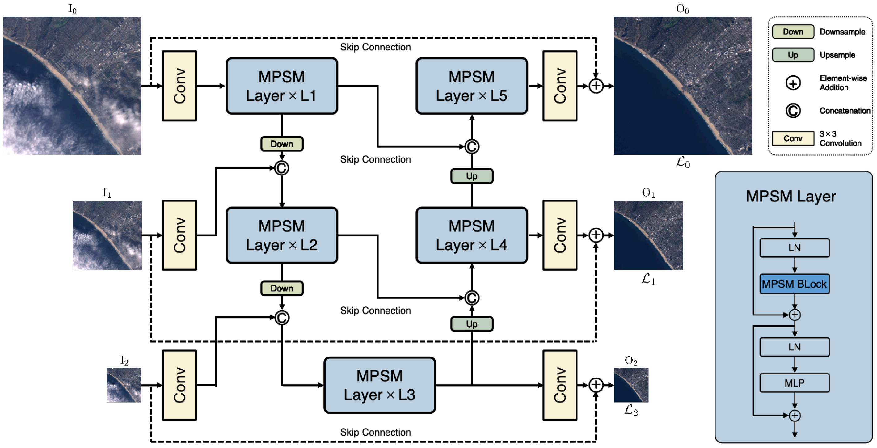
Figure 1. Overall framework. It is a U-net-style framework that integrates the proposed multi-pattern scanning Mamba layer and convolutional layer into an encoder–decoder architecture with multi-scale supervision. The dashed line denotes the skip connection from the original input image.
Remotesensing 17 03593 g001
Figure 2. Illustration of the proposed multi-pattern scanning Mamba block. (a) The vanilla Mamba Block. (b) The multi-pattern scanning Mamba block (MPSM Block). (c) The multi-pattern scanning 2D (MPS2D) module. (d) The ScanPattern module. (e) The dynamic path-aware (DPA) module.
Remotesensing 17 03593 g002
Figure 3. Three sequential patterns—Zigzag, Snake, and Diagonal. Each pattern includes four scan paths starting from a different corner of the 2D image: top-left, top-right, bottom-right, and bottom-left.
Remotesensing 17 03593 g003
Figure 4. Qualitative results on RICE1. The content inside the red box in the image represents an enlarged view of the content within the green box.
Remotesensing 17 03593 g004
Figure 5. Qualitative results on RICE2. The content inside the red box in the image represents an enlarged view of the content within the green box.
Remotesensing 17 03593 g005
Figure 6. Qualitative results on T-CLOUD. The content inside the red box in the image represents an enlarged view of the content within the green box.
Remotesensing 17 03593 g006
Figure 7. Comparison of qualitative results obtained using different scanning patterns on RICE2.
Remotesensing 17 03593 g007
Figure 8. Qualitative visualization of cloud-removal results under different cloud conditions and diverse land-cover backgrounds.
Remotesensing 17 03593 g008
Table 1. Configuration of the multi-pattern scanning Mamba framework.
StageOperationIn SizeOut SizeK/S
I 0 Conv H × W × 3 H × W × C 3/1
Encoder 0 MPSM Layer × 1 H × W × C H × W × C 3/1
Down 0 Inp, Conv, Cat H × W × C H 2 × W 2 × 2 C 3,1/1
I 1 Conv H 2 × W 2 × 3 H 2 × W 2 × C 3/1
Encoder 1 MPSM Layer × 2 H 2 × W 2 × 2 C H 2 × W 2 × 2 C 3/1
Down 1 Inp, Conv, Cat H 2 × W 2 × 2 C H 4 × W 4 × 4 C 3,1/1
I 2 Conv H 4 × W 4 × 3 H 4 × W 4 × C 3/1
Encoder 2 MPSM Layer × 8 H 4 × W 4 × 4 C H 4 × W 4 × 4 C 3/1
O 2 Conv, Add H 4 × W 4 × 4 C H 4 × W 4 × 3 3/1
Up 1 Conv, Cat H 4 × W 4 × 4 C H 2 × W 2 × 2 C 3/1
Decoder 1 MPSM Layer × 2 H 2 × W 2 × 2 C H 2 × W 2 × 2 C 3/1
O 1 Conv, Add H 2 × W 2 × 2 C H 2 × W 2 × 3 3/1
Up 0 Conv, Cat H 2 × W 2 × 2 C H × W × 2 C 3/1
Decoder 0 MPSM Layer × 1 H × W × 2 C H × W × 2 C 3/1
O 0 Conv, Add H × W × 2 C H × W × 3 3/1
Notations: C  = channels, H  = height, W  = width, Up = Upsample, Down = Downsample, Inp = Interpolation, Cat = Concatenation, Add = Element-wise Addition, K/S = Kernel/Stride.
Table 2. The characteristics of the RICE1, RICE2, and T-CLOUD datasets used in our experiments.
DatasetSourceSizeTrainingTesting
RICE1 [51]Google Earth512 × 512400100
RICE2 [51]Landsat 8512 × 512588147
T-CLOUD [11]Landsat 8256 × 2562351588
SEN12MS-CR [52]Sentinel series satellites256 × 256114,3257893
Table 3. Quantitative comparison results on RICE1, with the best results in bold. ↓: the lower the better, ↑: the higher the better. Our method achieves the best performance across all evaluation metrics with competitive computational efficiency.
MethodBackboneRICE1Overhead
MAE↓SAM↓PSNR↑SSIM↑Param (M)FLOPs (G)
pix2pix [7]CNN0.02534.1131.970.916154.416.1
SPA-GAN [26]0.03722.2528.890.91440.2115.2
RCA-Net [25]0.09065.2623.020.90013.09402.3
CVAE [11]Transformer0.01981.1133.700.956215.4237.1
Restormer [19]0.01761.0135.420.961726.13155.0
Trinity-Net [16]0.03052.2030.120.960520.2417.6
CMNet [17]0.01440.9936.200.961916.51236.0
CR-former [20]0.01410.9536.560.962017.1860.89
CR-Famba [42]Mamba0.03251.6430.910.9142174.94165.0
Ours0.01400.9236.650.96254.2732.6
Table 4. Quantitative comparison results on RICE2, with the best results in bold. ↓: the lower the better, ↑: the higher the better. Our method achieves the best performance across all evaluation metrics with competitive computational efficiency.
MethodBackboneRICE2Overhead
MAE↓SAM↓PSNR↑SSIM↑Params (M)FLOPs (G)
pix2pix [7]CNN0.03275.0829.450.847354.416.1
SPA-GAN [26]0.04033.3627.510.81770.2115.2
RCA-Net [25]0.137410.2816.480.79423.09402.3
CVAE [11]Transformer0.02161.6933.620.907915.4237.1
Restormer [19]0.01631.2736.050.915526.13155.0
Trinity-Net [16]0.02952.6330.090.877120.2417.6
CMNet [17]0.01671.2935.820.915116.51236.0
CR-former [20]0.01611.2836.210.915117.1860.89
CR-Famba [25]Mamba0.02522.2331.900.8495174.94165.0
Ours0.01561.2136.380.91684.2732.6
Table 5. Quantitative comparison results on T-CLOUD, with the best results in bold. : the lower the better, : the higher the better. Our method shows the best performance across four evaluation metrics while maintaining relatively low computational complexity.
MethodBackboneT-CLOUDOverhead
MAE↓SAM↓PSNR↑SSIM↑Params (M)FLOPs (G)
pix2pix [7]CNN0.044910.0125.640.756354.416.1
SPA-GAN [26]0.04194.0926.140.79540.2115.2
RCA-Net [25]0.06923.9023.380.81553.09402.3
CVAE [11]Transformer0.03422.9528.190.861315.4237.1
Restormer [19]0.02482.4630.490.885126.13155.0
Trinity-Net [16]0.03653.6727.330.841020.2417.6
CMNet [17]0.02512.4930.320.882316.51236.0
CR-former [20]0.02422.4630.600.883817.1860.89
CR-Famba [42]Mamba0.02622.4830.100.8810174.94165.0
Ours0.02372.3630.820.88874.2732.6
Table 6. Quantitative comparison and computational overhead on the SEN12MS-CR dataset. : the lower the better, : the higher the better. Best results are highlighted in bold.
ModelMAE↓SAM↓PSNR↑SSIM↑Param (M)FLOPs (G)
pix2pix [7]0.03110.78427.600.86454.416.1
SPA-GAN [26]0.04518.08524.780.7540.2115.2
DSen2-CR [58]0.0319.47227.760.87418.921240.2
GLF-CR [15]0.0288.98128.640.88514.82250.0
UnCRtainTS [59]0.0278.32028.900.8800.5637.1
Ours0.0268.22029.590.8934.2732.6
Table 7. Ablation study of combined scanning patterns on RICE2, with the best results in bold. ↓: the lower the better, ↑: the higher the better.
ComponentsRICE2Overhead
ZigzagSnakeDiagonalMAE↓SAM↓PSNR↑SSIM↑Param (M)FLOPs (G)
××0.01621.2835.870.91594.3833.45
××0.01651.2535.940.91594.3833.45
××0.01661.2635.750.91554.3833.45
×0.01601.2536.020.91664.3032.82
×0.01641.2935.870.91534.3032.82
×0.01621.2735.970.91524.3032.82
0.01571.2536.070.91754.2732.60
Table 8. Comparison between the vanilla Mamba block and the proposed MPSM block under the same U-Net framework, together with an ablation study of the dynamic path-aware (DPA) mechanism and multi-scale loss ( L M S ) on RICE2, with the best results in bold. ↓: lower is better; ↑: higher is better.
ModelsComponentsRICE2Overhead
MAE↓SAM↓PSNR↑SSIM↑Param (M)FLOPs (G)
U-Net (Vanilla
Mamba)
-0.01621.2835.870.91594.3833.45
w/o DPA0.01571.2536.070.91754.2732.60
U-Net (MPSM)w/o L M S 0.01591.2436.250.91594.2632.53
full0.01561.2136.380.91684.2732.60
Table 9. Comparison of computational overhead on NVIDIA RTX 3090 GPU with input resolution 256 × 256 . Lower values indicate better efficiency.
ModelBackboneParam (M)FLOPs (G)Time (ms)Memory (MB)
pix2pix [7]CNN54.416.14.603357
SPA-GAN [26]0.2115.226.003749
CVAE [11]Transformer15.4237.115.101097
Restormer [19]26.13155.0112.301629
CMNet [17]16.51236.0197.001607
CR-Former [20]17.1860.872.881561
CR-Famba [42]Mamba174.94165.0119.541716
Ours4.2732.675.781094
Table 10. Quantitative performance and computational overhead of the proposed model on RICE2 under different input resolutions on NVIDIA RTX 3090 GPU. ↓: the lower the better, ↑: the higher the better.
Image ResolutionMAE↓SAM↓PSNR↑SSIM↑Param (M)FLOPs (G)Time (ms)GPU Memory (MB)
2048 × 20480.02391.5833.270.96434.272117.636675.4337154
1024 × 10240.01881.3435.190.94724.27534.531128.419664
768 × 7680.01671.2535.980.93934.27300.03522.975666
512 × 5120.01571.2536.070.91754.27133.12191.862798
384 × 3840.01521.2036.560.91864.2773.34105.051802
256 × 2560.01571.2636.240.90464.2732.6075.781094
128 × 1280.01881.1534.620.86964.278.1565.10704
64 × 640.02491.8932.180.84064.272.0362.53644
32 × 320.03542.5928.560.80984.270.5154.72510
Disclaimer/Publisher’s Note: The statements, opinions and data contained in all publications are solely those of the individual author(s) and contributor(s) and not of MDPI and/or the editor(s). MDPI and/or the editor(s) disclaim responsibility for any injury to people or property resulting from any ideas, methods, instructions or products referred to in the content.