Highlights
What are the main findings?
- Deep learning models achieved R2 = 0.82 for canopy height prediction in Indonesian Borneo, substantially outperforming traditional tree-based algorithms (R2 = 0.57–0.58) and representing a significant advancement over recent tropical forest studies (R2 = 0.6–0.75).
- A comprehensive multi-source remote sensing approach integrating Landsat-8, Sentinel-1 SAR, DEM, and bioclimatic variables enabled accurate canopy height mapping across 2 million data points with 336 features, demonstrating the potential of large-scale data fusion for forest structural monitoring.
What is the implication of the main finding?
- This framework provides a cost-effective alternative to expensive LiDAR mapping for forest monitoring applications, enabling stakeholders to track canopy height changes over time using freely available satellite data across broad tropical forest regions.
- The high-resolution canopy height maps generated across diverse Borneo forest ecosystems (dipterocarp, peat swamp, montane) demonstrate the framework’s versatility and potential for operational forest monitoring, carbon accounting, and conservation planning across tropical regions.
Abstract
Accurate mapping of forest canopy height is essential for monitoring forest structure, assessing biodiversity, and informing sustainable management practices. However, obtaining high-resolution canopy height data across large tropical landscapes remains challenging and prohibitively expensive. While machine learning approaches like Random Forest have become standard for predicting forest attributes from remote sensing data, deep learning methods remain underexplored for canopy height mapping despite their potential advantages. To address this limitation, we developed a rapid, automatic, scalable, and cost-efficient deep learning framework that predicts tree canopy height at fine-grained resolution (30 × 30 m) across Indonesian Borneo’s tropical forests. Our approach integrates diverse remote sensing data, including Landsat-8, Sentinel-1, land cover classifications, digital elevation models, and NASA Carbon Monitoring System airborne LiDAR, along with derived vegetation indices, texture metrics, and climatic variables. This comprehensive data pipeline produced over 300 features from approximately 2 million observations across Bornean forests. Using LiDAR-derived canopy height measurements from ~100,000 ha as training data, we systematically compared multiple machine learning approaches and found that our neural network model achieved canopy height predictions with R2 of 0.82 and RMSE of 4.98 m, substantially outperforming traditional machine learning approaches such as Random Forest (R2 of 0.57–0.59). The model performed particularly well for forests with canopy heights between 10–40 m, though systematic biases were observed at the extremes of the height distribution. This framework demonstrates how freely available satellite data can be leveraged to extend the utility of limited LiDAR coverage, enabling cost-effective forest structure monitoring across vast tropical landscapes. The approach can be adapted to other forest regions worldwide, supporting applications in ecological research, conservation planning, and forest loss mitigation.
1. Introduction
1.1. Forest Structure Monitoring in Tropical Ecosystems
Tropical forests play a crucial role in global ecology, serving as biodiversity hotspots and significant carbon reservoirs. These ecosystems are under threat, with deforestation and forest degradation in tropical countries accounting for approximately 10 percent of total global annual carbon emissions [1,2]. Local, national, and international initiatives (e.g., REDD+) have been established to conserve these forests and their ecological functions. Effectively monitoring these initiatives requires accurate assessment of forest structural attributes, particularly canopy height, which serves as a fundamental indicator of forest condition, habitat quality, and ecosystem services. Tree canopy height (TCH) is among the most informative structural characteristics of forests, strongly correlating with biodiversity metrics, biomass accumulation, forest succession stage, and habitat complexity [3]. As a directly measurable physical property, canopy height provides insights into forest dynamics that cannot be observed from conventional two-dimensional remote sensing approaches that primarily detect forest cover but not vertical structure. Accurate canopy height maps enable researchers and forest managers to characterize habitat suitability for canopy-dependent species, identify old-growth forest remnants, quantify forest degradation impacts, and monitor recovery following disturbance [3,4].
Beyond its ecological significance, canopy height is particularly valuable because it serves as the primary input for numerous forest assessment models, including carbon stock estimation. When combined with field measurements of wood density and basal area, height data can be incorporated into allometric equations to estimate aboveground carbon density [2,5]. This relationship has made canopy height mapping a priority for forest monitoring programs worldwide, including those focused on climate change mitigation through forest conservation.
1.2. Challenges in Forest Structure Measurement
Obtaining accurate forest structure measurements, particularly canopy height, presents significant challenges across tropical landscapes [2,6]. Traditional field methods for measuring canopy height rely on instruments such as clinometers, laser rangefinders, or hypsometers, which measure angles and distances to estimate tree heights [6]. These approaches require unobstructed views of both the tree base and crown, which is often difficult in dense tropical forests with complex understory vegetation. Digital hemispherical photography and terrestrial LiDAR scanning offer more sophisticated alternatives but still require significant field effort [7].
Field campaigns to comprehensively characterize forest structure typically require teams of 5–10 technicians working for weeks to measure structural traits (e.g., tree heights, trunk diameters, crown dimensions) over relatively small areas of a few hectares [2]. This resource-intensive process limits the spatial extent and frequency of measurements. While these field methods provide accurate point-based estimates, extrapolating canopy height and other structural metrics beyond measured plots remains challenging, as it requires inferring information across vast, often inaccessible landscapes with heterogeneous topography and forest composition [8].
The limitations of field-based approaches are particularly problematic for tropical forests, which encompass over 1.8 billion ha globally [9]. These forests are often located in remote regions with limited infrastructure, creating logistical challenges for field campaigns. Additionally, the exceptional vertical complexity of tropical forests, with canopies frequently exceeding 40 m and complex multi-layered structures, introduces measurement difficulties not encountered in other forest types. This complexity makes tropical forests simultaneously among the most important ecosystems to monitor and among the most challenging to measure accurately using conventional methods.
1.3. Remote Sensing Approaches for Canopy Height Mapping
The practical constraints of field measurements have spurred interest in remote sensing approaches, which offer greater spatial coverage and repeated temporal sampling. However, remote sensing of forest structure introduces its own methodological challenges, particularly in translating two-dimensional spectral information into meaningful three-dimensional structural metrics like canopy height. These challenges have driven the development of specialized sensors and analytical techniques specifically designed to capture forest structural properties across broad spatial scales [10].
Currently available platforms like Hansen Global Forest Watch (GFW) [11] provide valuable data on forest cover change at global scales. While GFW effectively detects forest loss and gain patterns, it primarily offers two-dimensional information about forest extent rather than vertical structure. This limitation means that important structural transitions—such as selective logging, forest degradation, or regrowth stages—that significantly affect canopy height without changing forest/non-forest classification remain undetected [11]. These structural changes are particularly important in tropical forest monitoring, as they often precede complete deforestation and represent significant ecological transitions.
Airborne Light Detection and Ranging (LiDAR) technology has revolutionized forest structure assessment by providing high-definition, three-dimensional data on canopy height and structure [7,12]. LiDAR systems emit laser pulses that reflect off forest canopies and underlying terrain, enabling precise measurement of vegetation height, density, and arrangement. This technology can penetrate gaps in the canopy to create detailed profiles of forest structure from the ground to the uppermost leaves. LiDAR-derived canopy height has been successfully used to characterize forest structure across diverse tropical regions, including Central America [13], South America [14], Asia [15], Africa [16,17,18], and oceanic islands [19].
Despite its exceptional accuracy, airborne LiDAR coverage remains geographically limited due to the substantial costs and logistical challenges associated with aircraft-based remote sensing campaigns [19,20]. A typical LiDAR acquisition mission costs between $300-$550 per square kilometer [21], making wall-to-wall coverage prohibitively expensive for most tropical forest regions. These constraints have driven efforts to integrate LiDAR with other remote sensing technologies, particularly satellite-based optical and radar sensors, which offer broader spatial coverage at lower cost, albeit with reduced structural detail [1,14,22,23].
The integration of airborne LiDAR with satellite imagery and other geospatial datasets has emerged as a promising approach for extending high-resolution canopy height mapping beyond limited LiDAR footprints [24,25]. This synergistic approach leverages the structural detail of LiDAR samples with the comprehensive coverage of satellite data. For example, Asner et al. [26] combined Landsat-derived spectral information with Shuttle Radar Topography Mission elevation data to model forest structure in Peru, while Baccini and Asner [27] integrated MODIS imagery with LiDAR samples to produce pantropical canopy height maps. Notably, Mascaro et al. [12] pioneered the application of machine learning algorithms to this data fusion approach, demonstrating significant improvements in canopy height prediction accuracy. These advances have established a foundation for more sophisticated modeling approaches that combine diverse remote sensing inputs to map forest structure across large geographical extents.
1.4. Machine Learning for Forest Canopy Height Prediction
The challenge of predicting forest canopy height from satellite imagery has increasingly been addressed through machine learning (ML) techniques, which can identify complex, non-linear relationships between spectral/textural features and forest structural attributes [28,29,30,31,32]. These computational approaches offer a promising avenue to translate the wealth of available satellite data into ecologically meaningful structural metrics across broad spatial scales.
Random Forest (RF) has emerged as the leading ML approach for forest structure mapping due to its non-parametric nature and robustness when handling skewed data distributions and large feature sets typical of remote sensing datasets [33]. This algorithm constructs multiple decision trees using bootstrapped samples and random feature subsets, then aggregates their predictions to reduce overfitting and improve generalizability across diverse forest conditions. The predictive power of ML approaches can be substantially enhanced by incorporating spatial texture metrics derived from satellite imagery, particularly Fourier transform textural ordination (FOTO) [34,35] and gray-level co-occurrence matrices (GLCMs) [36,37,38], which capture spatial patterns that often correlate strongly with forest structural complexity.
Despite RF’s dominance in forest applications, recent advances in ML have introduced promising alternatives that remain underexplored for canopy height prediction. Gradient boosting frameworks such as XGBoost [39] and LightGBM [40] have demonstrated exceptional performance in other remote sensing applications but have not been comprehensively evaluated for forest structure mapping. Similarly, deep learning approaches—particularly neural networks—have revolutionized many computer vision tasks by automatically learning hierarchical feature representations from data [41] yet remain underutilized for forest canopy height prediction compared to traditional ML algorithms [42]. As Kattenborn et al. (2021) [42] note in their comprehensive review, neural networks show exceptional promise for vegetation remote sensing but their application to forest structural mapping has been limited compared to other domains. Recent studies suggest that deep learning approaches may offer significant improvements for canopy height mapping by capturing more complex relationships within multi-source remote sensing datasets than is possible with conventional ML algorithms [41,42]. For example, Schwartz et al. (2025) [43] successfully employed deep learning models with U-Net architecture to produce high-resolution canopy height maps across France, demonstrating that these advanced approaches can effectively integrate multi-source remote sensing data for forest structure monitoring. This growing body of evidence suggests that deep learning methods deserve greater attention in tropical forest monitoring applications.
The integration of diverse remote sensing data sources presents both opportunities and challenges for ML-based canopy height mapping. Combining multiple sensors with derived indices and ancillary environmental data provides complementary information about forest structure but creates high-dimensional feature spaces that may lead to overfitting. Addressing these challenges requires careful feature selection, regularization techniques, and robust validation approaches to ensure model generalizability across diverse forest conditions [44].
In this study, we present an open-source, rapid, automated, and cost-efficient framework to accurately predict tree canopy height across tropical forests. By integrating multiple sources of satellite imagery and remotely sensed data with high-resolution LiDAR-derived canopy height measurements, we have trained and compared various ML algorithms, including tree-based models and deep learning neural networks. We hypothesized that a deep learning model would outperform traditional tree-based algorithms by better capturing complex relationships within our large, multi-source feature set. Our approach achieves significantly higher accuracy than previous methods, demonstrating that freely available remote sensing data can be leveraged to extend limited LiDAR coverage for large-scale forest structure mapping. While our primary focus is accurate canopy height prediction, these estimates could potentially support carbon stock assessment in regions where appropriate allometric relationships exist, though that application would require additional validation beyond the scope of this study.
2. Materials and Methods
2.1. Study Area and Data Pipeline
Borneo, a 750,000 km2 island, contains some of the world’s most biodiverse and carbon-dense tropical forests. The island is predominantly covered by lowland dipterocarp rainforests, with significant areas of peat swamp forests, mangroves along coastal regions, and montane forests at higher elevations. However, Borneo has lost about 30% of its forests within the last 40 years [45]. In 2014, the NASA Carbon Monitoring System (CMS) surveyed 85 sites in Indonesian Borneo (Kalimantan) using plane-based LiDAR [46] (Figure 1). These surveys, covering approximately 100,000 ha, utilized a Riegl LMS-Q680i sensor, acquiring data at point densities between 4 and 10 points per square meter. The data were collected between 18 October and 30 November 2014, resulting in Digital Surface Models (DSMs), Digital Terrain Models (DTMs), and Canopy Height Models (CHMs) at 1-meter resolution. The LiDAR data processing was performed by the NASA CMS team using a multi-stage processing routine with the Point Data Abstraction Library (PDAL) to generate ground-classified point clouds and subsequently derive the CHMs [46]. We resampled these CHMs to 30-meter resolution using mean canopy height values within each 30 × 30 m pixel and used this information, along with hundreds of covariates derived from broadly available remote sensing products, as training data for a series of ML and DL prediction models.
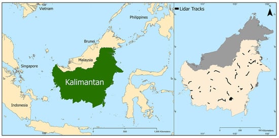
Figure 1.
(Left) Location of Indonesian Borneo (Kalimantan) in South-East Asia. (Right) NASA CMS LiDAR flight path locations, indicating LiDAR tracks (black color) in 85 sites in Indonesia Borneo.
While providing valuable data for this region, the limited spatial extent of the LiDAR data necessitates integrating it with other remote sensing data for broader applicability. Therefore, LiDAR is often paired with optical remote sensing data with varying spatial and spectral properties to model LiDAR-derived properties across larger geographical scales afforded by satellites [1,8,15,16]. Coupling airborne LiDAR with satellite images and other geospatial datasets has become a more common approach to map tropical forest aboveground carbon density (ACD), particularly in geographic regions lacking sufficient LiDAR measurements [17,18].
Like previous studies [12,47], we integrated several sources of common remote sensing data in our data pipeline, including Landsat-8 (8 spectral bands), Sentinel-1 (4 band Synthetic Aperture Radar), land cover fractional coverages from the Copernicus satellite mission, digital elevation model, and NASA CMS airborne LiDAR. Because of data loss due to cloud cover and other atmospheric effects, Landsat data were temporally sampled from August 2014–January 2015 (the time period of the LiDAR data plus 2 months before and after). We applied cloud masking to all Landsat imagery using the pixel QA band in Google Earth Engine, which employs the CFMask algorithm to identify clouds, cloud shadows, and other quality issues. Only pixels classified as clear in the QA band were included in our analysis. In addition to these data, we also integrated other data sources, such as indices commonly used to assess vegetation (e.g., NDVI, NDWI, NDII, EVI, for Landsat 8), Gray-Level Co-occurrence Matrix (GLCM) texture metrics [36] for all spectral data, and climatic data from WorldClim [48]. All these data sources (listed in Table 1) were compiled into a data processing pipeline which produced our dataset of 336 features for each LiDAR value (examples in Figure 2), resulting in about 2 million observations. The definition of each data feature is listed in Supplementary Material Table S1.

Table 1.
Data sources in the GEE data pipelines.
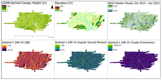
Figure 2.
Examples of data enrichment for a selected LiDAR track. (Top Left) Canopy height model derived from LiDAR. (Top Center) Elevation. (Top Right) NDVI median mosaic, contemporaneous with LiDAR flights. (Bottom Left) Sentinel-1 SAR. (Bottom Center) GLCM Angular Second Moment texture feature from Sentinel-1. (Bottom Right) GLCM Cluster Prominence texture feature from Sentinel-1. The other features are described in Table S1.
All data were reprojected to the coordinate reference system of the corresponding Landsat imagery (30 × 30 m pixel); LiDAR data were resampled using bicubic interpolation (Figure 3). Land Cover classification values were transformed via label encoding. This diverse remote sensing dataset was critical to providing the foundation on which we produced a robust, predictive ML framework. Here we utilized Google Earth Engine (GEE) [49] programmatically for data acquisition, processing, analysis, and modeling. The data processing pipelines we built in GEE can be further used to facilitate new data acquisition and processing for any future work in different forest regions or for scope expansion.
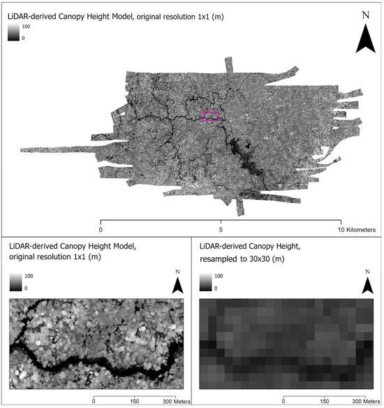
Figure 3.
(Top) An original full extent, full resolution (1 × 1 m) LiDAR-derived Canopy Height Model (CHM) with a rectangle (pink) showing the inset location. (Bottom Left) Zoomed-in inset of CHM at original 1 × 1 m resolution, showing individual trees as light-colored circular shapes and a river/low ground in dark. (Bottom Right) CHM image after resampling to Landsat-8 scale (30 × 30 m).
2.2. ACD Estimation
In this study, we focused on developing a model to predict average canopy height at the scale of the Landsat satellite constellation (30 × 30 m), providing a rapid and low-cost means of estimating forest stock in Borneo using only freely available remote sensing data. TCH can be used to calculate ACD for forests where the empirical relationship has been established, such as certain types of lowland tropical rainforests in Sepilok in Malaysian Borneo [15]. An example of this equation is as follows:
where ACD is in Mg C ha−1, TCH is in m, basal area (BA) is in m2 ha−1, and wood density (WD) is in g cm−3. Jucker et al. [15] combined field data of tree height measurements with airborne laser scanning and hyperspectral imaging to characterize how topography shapes the vertical structure, wood density, diversity and ACD of nearly 15 km2 of old-growth forest in Borneo. This general form of empirical relation was first developed by Asner et al. [14] and the allometric scaling coefficients in the equations are region-specific and are based on the field work that took place in that region. The error range of the ACD values calculated from the empirical equations is 39.3 Mg C ha−1 [15].
ACD = 0.567 × TCH0.554 × BA1.081 × WD0.186
BA = 1.112 × TCH
WD = 0.385 × TCH0.097
Since BA and WD exhibit high variation across forest types, and both forest types and terrain features (elevation, slope, topography) co-vary with ACD, it is necessary to develop specific ACD estimation equations for tree species while also considering the unique topographical distinctions between similar forests [15]. Gathering sufficient data to establish forest-specific allometric equations requires extensive investment in field data collection, which was beyond the scope of this current study. Our focus here was on accurate canopy height prediction, reproducing one of the three key variables for ACD estimation.
2.3. ML Framework
In our framework of TCH estimation from ML modeling, we experimented with several ML and DL algorithms, including artificial neural network [50], random forest (RF) [51], XGBoost [40], and LightGBM [41], as well as the most recent AutoMLs [52,53].
From our data pipeline, we ran each ML and DL algorithm with our dataset containing 336 features and 2 million TCH observations. The regression target for each ML model is the TCH value at the pixel level, representing the average canopy height in each 30 × 30-m grid cell. The goal was to develop a generalized ML model that can predict TCH solely based on open-source remote sensing data in the regions that LiDAR TCH is generally not available. The framework workflow is presented in Figure 4.
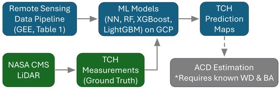
Figure 4.
ML framework with GEE remote sensing data pipeline and GCP infrastructure with ML model development and deployment for TCH prediction and optional ACD prediction. * ACD estimation requires additional information about Wood Density (WD) and Basal Area (BA) that is not directly predicted by our model.
The workflow for ML model development consisted of two stages: (1) training and validation and (2) testing. The selected ML model takes the input data (GEE compiled remote sensing data) and TCH as the predicted output values. During the training and validation phase, the cost (or loss) function based on the mean squared error (MSE), was used to evaluate the performance of the ML model by comparing the TCH estimation to the output values predicted by the ML model. Since this is a regression task, the evaluation metric we used here is Coefficient of determination (R2). We randomly split the dataset into a 90% training subset, a 5% validation subset, and a 5% test set. The subsets were kept consistent for each round of experiment of the selected ML algorithms. The validation set was used to evaluate if the model is over-fitting to the training data, while the test set was treated as out-of-bag data that were not used in the training phase.
Note that in general, with large datasets (e.g., >1 million data points), the artificial neural network (ANN) model is more generalizable and likely has higher predictive performance than the tree-based algorithms, such as RF. As RF has been tested rigorously in the remote sensing literature in recent years, we treat the tree-based algorithms tested in this study as the baseline.
We used Python version 3.8.20 to establish our code base and ML framework. The ML computation, model training, and inference were done in Google Cloud Platform’s Vertex AI.
2.3.1. Tree-Based Models
In addition to commonly used RF in the remote sensing community, we experimented with gradient boosted tree algorithms, such as XGBoost and LightGBM, as they have previously been effective in remote sensing image analysis and classifications of forests and land cover [54,55,56].
RF is a supervised ensemble algorithm that generates unpruned classification trees to predict a response [51]. RF implements bootstrapping samples of the data and randomized subsets of predictors. Final predictions are ensembled across a forest of classification trees (n = 100) based on an averaging of the probabilistic prediction of each classifier. Tree depth, number of leaf nodes, and number of features are tested with the dataset in each iteration in the training process.
XGBoost (eXtreme Gradient Boosting) is designed for both linear and tree-based supervised models [40]. XGBoost builds an ensemble of weak learners, where each weak learner is a decision tree. These decision trees are trained in a sequential manner, with each tree trying to correct the mistakes of the previous tree. The final output is a combination of all the individual trees, which results in a highly accurate model. XGBoost also includes a variety of regularization techniques, such as L1 and L2 regularization, and the ability to handle missing values and categorical variables.
Like XGBoost, LightGBM also builds an ensemble of weak learners, where each weak learner is a decision tree [41]. The key difference between LightGBM and XGBoost is the way they handle the decision tree learning process. LightGBM uses a technique called gradient-based one-side sampling to sample the data, which improves the speed of the training process. It also uses an algorithm called exclusive feature bundling to handle categorical variables, which reduces the number of splits required in the decision tree. Another difference between LightGBM and XGBoost is that LightGBM uses a leaf-wise tree growth algorithm, whereas XGBoost uses a level-wise tree growth algorithm. The leaf-wise algorithm tends to grow deeper trees than the level-wise algorithm, which results in better accuracy but can also lead to overfitting if not carefully controlled.
All tree-based models were initialized with hyperparameters typical for remote sensing applications. Specifically, RF was configured with 100 trees (n_estimators = 100) and a maximum depth of 10 (max_depth = 10). XGBoost and LightGBM were both configured with 100 trees (n_estimators = 100), maximum depth of 6 (max_depth = 6), and learning rate of 0.1 (learning_rate = 0.1). These parameters represent a balance between model complexity and computational efficiency while maintaining robust predictive performance.
2.3.2. Neural Network Models
Deep-learning algorithms (i.e., neural network models) have previously been effective for discovering underlying patterns in large datasets [50]. Therefore, we expected that neural network models could find highly predictive features from our diverse remote sensing data, which contained many data features (336) and data points (2 million). We specifically constructed the simple form of feedforward artificial neural network (ANN).
Feedforward ANNs consist of inter-connected computational units referred to as neurons that are arranged in layers. Input data are passed in one direction through an input layer and subsequently propagated through a defined number of hidden layers whereby the sum of the products of the connection weights from each layer approximate a function to estimate the observed output values [50]. Under repeated iteration and adjustment of the connection weights, a function between inputs and output is as closely estimated as possible given the parameter space available in the network [57,58]. Detailed development of model architecture lies in the selection of node functions (i.e., activation functions), layer sizes (number of hidden layers and numbers of nodes in each layer), learning rate, regularization parameters, and parameter dropout, which is discussed in Section 2.3.3.
As described above, the neural network used the input parameters as the first layer of neurons, and the last layer of neurons represents the predicted output values. Stochastic gradient descent, a common optimization method for ANN, was then used to iteratively adjust the weights and biases for each neuron to allow the ANN to best approximate the training data output. At each iteration, a backpropagation algorithm estimated the partial derivatives of the cost function (MSE) with respect to incremental changes of all the weights and biases, to determine the gradient descent directions for the next iteration. Note that in our model, the neurons of each hidden layer were composed of Rectified Linear Units (i.e., a ReLU activation function), to avoid the vanishing gradients [59]. Validation data were not used in the optimization or backpropagation algorithms. Instead, the cost function was evaluated over the validation data and served as an independent tuning metric of the performance of the ANN.
2.3.3. AutoML (Automated Machine Learning)
AutoML (Automated Machine Learning) is a technique that automates the process of building machine learning models, from data preparation to model selection and hyperparameter tuning [52]. The goal of AutoML is to make the process of building models more accessible and efficient for ML practitioners [53]. In this study, we primarily utilized AutoML for model selection and fine-tuning, as manually constructing the architecture of an ANN model and fine-tuning hyperparameters, such as number of hidden layers, numbers of nodes in each layer, learning rate, and dropout rate, can be a time-consuming and complex process. We implemented a Python library, Auto-Keras [60], to automate the search process for ANN architecture that yields the best model prediction R2. To evaluate the robustness of the ANN model, we compared it to the best-performing tree-based model as our baseline. We implemented a Python library, TPOT, a tree-based pipeline optimization tool for automating machine learning [61], to automate the search process for tree-based models that yielded the best model prediction R2.
3. Results
In our experiments, with 336 data features and 2 million data points on TCH compiled from our GEE processing, the tree-based ML models achieved good R2 performance on the test set. Our tree-based baseline ML models all have similar and consistent predictive performance: R2 = 0.572 for the RF model, 0.583 for the XGBoost model, and 0.581 for the LightGBM model. TPOT, the AutoML approach, found the best tree-based model to be the decision tree with fine-tuned parameters (maximum depth = 9, minimum sample leaf = 2, minimum samples split = 15) and the best R2 was 0.593. These results are better than the comparable studies [12,62], here used as benchmark (R2 of 0.3–0.5), due to the large number of features used in our study. For instance, the RF model in Mascaro et al. [12] was trained with data that contained only multispectral satellite channels and land cover features, which had a total of 11 data features and 80,000 data points.
As our models were not built for interpretability, but rather to maximize predictive power by including many features, it is of limited use to select a single feature and comment on its significance. However, we did calculate the feature importance from the RF, XGBoost, and LightGBM models. The 3 most important features of each model are presented in Table 2. In general, the top features that have the most predictive power for the TCH estimation were Sentinel-1 VH Cluster Shade (a GLCM texture feature), Landsat-8 thermal and infrared GLCM features, and Landsat-8 Red and Blue GLCM features. GLCM features comprised the top 5 features of every model run, which indicates the significance of texture analysis of medium-scale satellite imagery in the analysis of forest canopy structure.
Table 2.
Tree-Based Models Top 3 Features.
For the DL experiments, the AutoML approach via Auto-Keras found the best neural network model to be 3 dense layers that applied multi-category encoding and normalization; each hidden layer had 32 neurons. The model used Adam optimizer with a learning rate of 0.001 and batch size of 32. During the AutoKeras search process, the algorithm explored architectures ranging from 1 to 10 layers, with 16 to 512 neurons per layer, and learning rates between 0.0001 and 0.1, with a maximum of 5 trials and 100 training epochs per trial. ReLU activation function layers are implemented twice in this best-fit model, which allows the neural network to learn hierarchical non-linear representations of the input data. The model architecture summary is presented in Table 3. This neural network had 13,090 total parameters in which 12,385 parameters were trainable. This custom feed-forward ANN achieved R2 = 0.821 on the test set, which is higher than our tree-based baseline models and outperformed comparable studies [12,62]. Overall RMSE was 4.98 m and MAE was 3.55 m.
Table 3.
Neural network model summary.
Most (96%) of the forest samples in our dataset had TCH values under 40 m, with over half (56%) in the 10–30 m range. This right-skewed distribution with a long tail is typical of tropical forests, and we found that our model struggled with the taller height classes, with RMSE increasing dramatically as TCH increases above 40 m (Figure 5). Additionally, shorter canopy heights were systematically overestimated (positive bias up to 2.9 m in the 0–30 m range), while very tall canopy heights were substantially underestimated (negative bias exceeding −50 m for trees > 80 m). This is to be expected due to the heavy imbalance in height distribution and is a classic example of regression towards the mean.
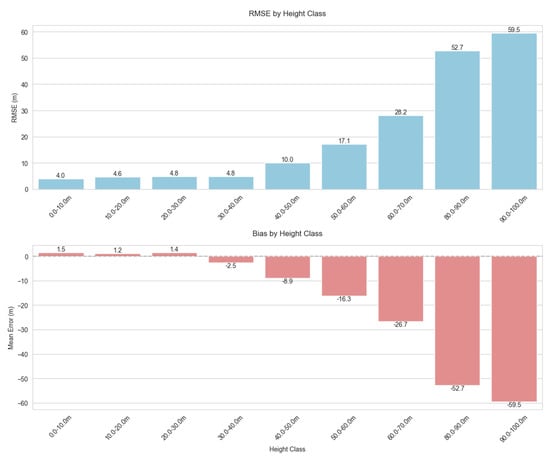
Figure 5.
Distribution and trends of model prediction errors by 10 m binned canopy height classes. The model performed consistently well across the most common height ranges (10–40 m), with performance degrading for extreme and rare values.
After obtaining the best neural network model, we used it to produce a prediction TCH map over a section of Bornean forest not used in model training. As an example of the potential application for ACD estimation, the allometric equation was applied and visualized (Figure 6).
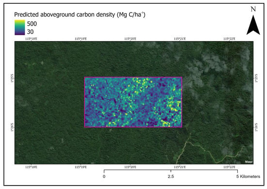
Figure 6.
Section of forest in Indonesia Borneo with estimated aboveground carbon density visualized. The pink box indicates the area where our deep learning model was applied to predict carbon density values. The same trained model can be applied to any forested area in Indonesian Borneo that does not have LiDAR data. Note: this figure is not intended to be an accurate estimation of ACD in this particular forest patch.
4. Discussion
Here we show that large remote sensing datasets incorporated into ML models demonstrate high predictive accuracy for forest canopy height. LiDAR data are increasingly used to monitor forest stock and carbon mapping, but it is expensive to gather. However, hundreds of other remote sensing-derived variables are freely available to the public, and we have shown the potential to use the available data to predict LiDAR-derived canopy height data across a broad region. As our model can reproduce the canopy height variable in areas lacking LiDAR coverage, using only the freely available predictors, this framework can be applied to other areas of Kalimantan, or adapted for other regions with partial LiDAR coverage, and can allow stakeholders to monitor forest canopy over time.
Our neural network approach (R2 = 0.82, RMSE = 4.98 m) represents a significant advancement in canopy height prediction accuracy compared to recent studies in tropical forests. In tropical contexts, Csillik et al. (2019) [63] reported R2 of 0.75 using random forest with PlanetScope imagery in Peru, while Potapov et al. (2021) [64] achieved R2 of 0.6–0.7 when mapping canopy height across the tropics using a combination of GEDI LiDAR and Landsat data. The higher accuracy of our approach likely stems from both our comprehensive feature engineering and the application of deep learning to a large, diverse dataset derived from multiple sensors.
Our three tree-based ML models trained with 336 data features and 2 million data points all had R2 values greater than 0.57, which is higher than prior studies with fewer features and data points that had R2 values in the 0.3–0.5 range [12,62]. This resonates with the recent data-centric AI approach, which emphasizes the importance of improving data quality and quantity, instead of focusing on improving ML algorithms [65,66,67].
We also found that our deep-learning neural-network model yielded substantially higher R2 than the tree-based models (R2 > 0.8). This is consistent with previous studies that showed that neural networks are more generalizable and capable of extracting underlying patterns from a large dataset, resulting in a higher predictive performance [68]. This is a large benefit, but there is also a cost, because neural network models are more difficult to interpret than tree-based models. While it is mathematically possible to determine which nodes of a deep neural network were activated, it is difficult to assess how each of the neuron layers performed collectively. This is less straightforward than interpreting conventional tree-based models, which provide crisp rules on feature selections and encode for feature importance, making it easier to interpret the reasoning behind the model. In this study, we focus more on model predictive performance than interpretability, though we recognize the trade-offs this entails for operational contexts where model transparency may be valued for stakeholder engagement and scientific communication. The substantial improvement in accuracy (R2 increase from 0.58 to 0.82) justified this approach, as it enables more reliable forest structure monitoring across large landscapes. Future work could explore interpretable deep learning techniques or hybrid approaches that maintain high accuracy while providing more transparent feature importance.
Our DL model, while relatively accurate, displayed high errors and negative bias among very tall forest patch samples (TCH > 40 m). This behavior can be explained by the dominance of mid-range samples (10–30 m), as the model is optimized to minimize overall error across all samples. Additionally, spectral bands from satellite sensors tend to saturate at higher canopy densities and heights, leading to a ceiling effect where differentiating between tall and very tall trees becomes challenging. Among the shortest TCH samples (TCH < 30 m), the model demonstrated a positive bias in predictions, which can be explained by the asymmetric prediction space created by the natural boundary at zero height, allowing positive errors only for the shortest trees.
This pattern of systematic bias in our model has significant implications for forest monitoring. Carbon stock estimates may be substantially underestimated in areas with mature forests, as biomass typically scales non-linearly with height, potentially leading to significant carbon accounting errors in old-growth stands. Our results show that for the tallest forest classes (80–90 m), the model underestimates height by an average of 52.7 m, which is a severe bias. Using the allometric equations from Jucker et al. (2018) [15], we estimate that such extreme underestimation could translate to approximately 65–75% underestimation of aboveground carbon density in these rare but ecologically important tall forest stands. For example, in a pristine dipterocarp forest with true canopy height of 85 m and expected ACD of 200 Mg C ha−1, our model’s predictions might suggest only 50–70 Mg C ha−1, an error of 130–150 Mg C ha−1. While these extremely tall forests represent only a small fraction of our study area (<1% of samples), they often contain disproportionately high carbon stocks and biodiversity values, making accurate estimation particularly important for conservation prioritization. Furthermore, the positive bias observed in shorter vegetation might mask subtle degradation signals when mature forest transitions to secondary growth, complicating forest degradation detection. From an ecological perspective, systematic height bias could result in misclassification of forest structural types, particularly misidentifying old-growth as secondary forest. In heterogeneous landscapes, these errors would manifest unevenly, creating artificial patterns in derived products that could mislead conservation planning. Additionally, when height estimates are incorporated into subsequent models for carbon, biodiversity, or ecosystem service assessments, these structured errors propagate and potentially amplify through non-linear transformations. Future work should explore bias correction functions calibrated to height classes, stratified modeling approaches, or ensemble methods weighted by height class representation to address these systematic biases in canopy height prediction. Statistical post-processing techniques such as quantile mapping or distribution-matching approaches could also help correct for the systematic biases observed at height extremes, potentially improving model utility for applications requiring accurate estimates across the full range of forest structures.
The humid tropical environment of Borneo presents specific challenges for canopy height mapping that our model had to navigate. The region’s heterogeneous forest ecosystems, ranging from lowland dipterocarp forests to peat swamps and montane formation, exhibit distinct structural characteristics that influence model performance. Dipterocarp-dominated forests, with their exceptionally tall emergent trees and complex vertical structure, likely contribute to the underestimation bias we observed in the tallest height classes. Meanwhile, peat swamp forests, with their unique spectral properties due to waterlogged conditions, may introduce additional variability in reflectance patterns that complicates height prediction. The persistent high humidity and frequent cloud cover across Borneo significantly constrain the availability of high-quality optical imagery, forcing our model to learn from a dataset with inherent temporal gaps and atmospheric noise. Despite these challenges, our approach demonstrated robust performance across the most common forest types, suggesting that deep learning methods can effectively capture the structural complexities of diverse tropical forest ecosystems through their ability to identify subtle patterns in multi-source data. Future refinements could include developing forest-type specific models or incorporating more detailed ecological stratification to account for the structural and spectral differences between Borneo’s distinct forest ecosystems.
For practical implementation by forest management stakeholders, our approach offers several advantages. The model can be deployed through cloud platforms like Google Earth Engine, allowing resource-constrained organizations to generate up-to-date canopy height maps without specialized computing infrastructure. These maps could be integrated into existing forest monitoring systems to detect structural changes too subtle to be captured by conventional forest/non-forest classifications. For example, selective logging operations that don’t create detectable gaps in Landsat imagery might still reduce mean canopy height by several meters, potentially detectable with our approach when applied to time-series data.
Note that the Landsat imagery used in our data pipeline is 30 m × 30 m, so the sub-meter LiDAR data were resampled to derive mean canopy height in each 30 m × 30 m grid cell. The new generation of high temporal and spatial resolution satellite data, e.g., PlanetScope, which began observations over Borneo in 2018, consists of pixel cell sizes at ~3–5 m2 and would thus reduce the amount of data resampling, potentially providing a better estimation of TCH and, in turn, of ACD [63]. PlanetScope sensors capture eight spectral bands, the same number as from Landsat, but don’t have a thermal infrared sensor. Nevertheless, in our models, texture features derived from red, blue, and infrared spectra consistently were ranked the most important, suggesting that PlanetScope sensors would still capture the most useful information, especially as the amount of textural information would increase greatly with the finer resolution. The use of PlanetScope imagery is particularly appealing as a future avenue of research because PlanetScope satellites now cover the entire globe daily, allowing high temporal frequency imagery of the area of interest in Borneo. This would greatly help with dealing with cloud cover, which is a common challenge in rainforests like the ones we considered in Borneo.
5. Conclusions
In this study, we developed a comprehensive framework for high-resolution forest canopy height mapping by integrating multi-source remote sensing data with machine learning approaches. By compiling an extensive dataset of 336 features from diverse sources including Landsat-8, Sentinel-1, land cover maps, digital elevation models, and derived indices, we trained models capable of accurately predicting tree canopy height across Indonesian Borneo’s complex tropical forest landscapes.
Our deep learning neural network model achieved an R2 of 0.82 and RMSE of 4.98 m, substantially outperforming traditional tree-based machine learning approaches (R2 = 0.57–0.59) and setting a new benchmark for canopy height prediction accuracy in tropical forests. This improvement demonstrates the value of both extensive feature engineering and advanced model architectures when working with complex ecological data. The model’s performance was particularly strong for forest patches with canopy heights between 10–40 m, which constitute the majority of the region’s forests, though systematic biases were observed at the extremes of the height distribution.
The framework we developed offers several key advantages for forest monitoring. First, it leverages freely available satellite data to extend the utility of limited LiDAR coverage, making high-resolution structural forest mapping financially feasible across large geographic regions. Second, our model provides the crucial canopy height variable that, when combined with validated region-specific allometric equations and field measurements, can support aboveground carbon density estimation, though such applications would require additional validation. Third, the automated processing pipeline can be modified for monitoring forest structure changes over time, potentially enabling the detection of subtle degradation not captured by conventional forest/non-forest classifications.
Several limitations of our approach highlight directions for future research. Addressing the systematic biases in height predictions for very tall and very short forests should be prioritized, potentially through stratified modeling approaches or ensemble methods. Statistical post-processing techniques such as quantile mapping or distribution-matching approaches could also help correct for the systematic biases observed at height extremes, potentially improving model utility for applications requiring accurate estimates across the full range of forest structures. To specifically address the substantial negative bias observed in extremely tall forest stands (>80 m), targeted field campaigns to collect ground-truthed height measurements in these rare but ecologically significant forest patches would enable the development of specialized correction factors or height-specific models. Additionally, investigating the transferability of this framework to other tropical forest regions would extend its global applicability. The integration of higher-resolution optical imagery from sources like PlanetScope could potentially improve prediction accuracy, particularly for capturing fine-scale forest heterogeneity.
Future efforts will focus on operationalizing this framework through cloud-based platforms like Google Earth Engine, making it accessible to forest managers, conservation organizations, and climate researchers. By providing accurate, up-to-date information on forest structure across large landscapes, this approach can contribute to more effective forest conservation strategies, support carbon stock assessments when combined with appropriate field data and inform climate mitigation policies in tropical forest regions worldwide.
Supplementary Materials
The following supporting information can be downloaded at: https://www.mdpi.com/article/10.3390/rs17213592/s1, Table S1: Definition for each feature in the dataset. References [69,70,71,72,73,74,75,76,77,78,79,80,81,82,83,84,85] are cited in the Supplementary Materials.
Author Contributions
Conceptualization, A.J.C., Z.Y.-C.L., S.H.S. and G.A.D.L.; Data curation, A.J.C.; Funding acquisition, G.A.D.L.; Investigation, A.J.C., Z.Y.-C.L., C.G.L.C., J.P., S.R.H. and S.H.S.; Methodology, A.J.C. and Z.Y.-C.L.; Project administration, G.A.D.L.; Supervision, S.H.S. and G.A.D.L.; Validation, A.J.C. and Z.Y.-C.L.; Visualization, A.J.C. and Z.Y.-C.L.; Writing—original draft, A.J.C. and Z.Y.-C.L.; Writing—review & editing, A.J.C., Z.Y.-C.L., C.G.L.C., J.P., I.Z.S., D.R.N., Y.S., K.W., S.R.H., S.H.S. and G.A.D.L. All authors have read and agreed to the published version of the manuscript.
Funding
This research was funded by a grant from the David and Lucile Packard Foundation (#2020-70906) and the National Geographic Society (#NGS-91292R-21), and Belmont Collaborative Forum on Climate, Environment and Health (NSF-ICER-2024383).
Data Availability Statement
Open-source dataset developed in this study can be accessed via this link (https://github.com/deleo-lab/carbon-remote-sensing-ml).
Acknowledgments
The authors would like to thank our institutions for providing facilities, resources, and administrative and technical support.
Conflicts of Interest
The authors declare no conflicts of interest.
Correction Statement
This article has been republished with a minor correction to resolve grammatical errors. This change does not affect the scientific content of the article.
References
- Baccini, A.; Goetz, S.J.; Walker, W.S.; Laporte, N.T.; Sun, M.; Sulla-Menashe, D.; Hackler, J.; Beck, P.S.A.; Dubayah, R.; Friedl, M.A.; et al. Estimated Carbon Dioxide Emissions from Tropical Deforestation Improved by Carbon-Density Maps. Nat. Clim. Change 2012, 2, 182–185. [Google Scholar] [CrossRef]
- Gibbs, H.K.; Brown, S.; Niles, J.O.; Foley, J.A. Monitoring and estimating tropical forest carbon stocks: Making REDD a reality. Environ. Res. Lett. 2007, 2, 045023. [Google Scholar] [CrossRef]
- Bergen, K.M.; Goetz, S.J.; Dubayah, R.O.; Henebry, G.M.; Hunsaker, C.T.; Imhoff, M.L.; Nelson, R.F.; Parker, G.G.; Radeloff, V.C. Remote sensing of vegetation 3-D structure for biodiversity and habitat: Review and implications for lidar and radar spaceborne missions. J. Geophys. Res. Biogeosci. 2009, 114, G00E06. [Google Scholar] [CrossRef]
- Davies, A.B.; Asner, G.P. Advances in animal ecology from 3D-LiDAR ecosystem mapping. Trends Ecol. Evol. 2014, 29, 681–691. [Google Scholar] [CrossRef] [PubMed]
- Chave, J.; Andalo, C.; Brown, S.; Cairns, M.A.; Chambers, J.Q.; Eamus, D.; Fölster, H.; Fromard, F.; Higuchi, N.; Kira, T.; et al. Tree Allometry and Improved Estimation of Carbon Stocks and Balance in Tropical Forests. Oecologia 2005, 145, 87–99. [Google Scholar] [CrossRef] [PubMed]
- Sullivan, M.J.P.; Lewis, S.L.; Hubau, W.; Qie, L.; Baker, T.R.; Banin, L.F.; Chave, J.; Cuni-Sanchez, A.; Feldpausch, T.R.; Lopez-Gonzalez, G.; et al. Field methods for sampling tree height for tropical forest biomass estimation. Methods Ecol. Evol. 2018, 9, 1179–1189. [Google Scholar] [CrossRef] [PubMed]
- Calders, K.; Adams, J.; Armston, J.; Bartholomeus, H.; Bauwens, S.; Bentley, L.P.; Chave, J.; Danson, F.M.; Demol, M.; Disney, M.; et al. Terrestrial laser scanning in forest ecology: Expanding the horizon. Remote Sens. Environ. 2020, 251, 112102. [Google Scholar] [CrossRef]
- Brearley, F.Q.; Adinugroho, W.C.; Cámara-Leret, R.; Krisnawati, H.; Ledo, A.; Qie, L.; Smith, T.E.L.; Aini, F.; Garnier, F.; Lestari, N.S.; et al. Opportunities and Challenges for an Indonesian Forest Monitoring Network. Ann. For. Sci. 2019, 76, 54. [Google Scholar] [CrossRef]
- FAO. Global Forest Resources Assessment 2020; FAO: Rome, Italy, 2020. [Google Scholar]
- Duncanson, L.; Armston, J.; Disney, M.; Avitabile, V.; Barbier, N.; Calders, K.; Carter, S.; Chave, J.; Herold, M.; Crowther, T.W.; et al. The Importance of Consistent Global Forest Aboveground Biomass Product Validation. Surv. Geophys. 2019, 40, 979–999. [Google Scholar] [CrossRef]
- Hansen, M.C.; Potapov, P.V.; Moore, R.; Hancher, M.; Turubanova, S.A.; Tyukavina, A.; Thau, D.; Stehman, S.V.; Goetz, S.J.; Loveland, T.R.; et al. High-Resolution Global Maps of 21st-Century Forest Cover Change. Science 2013, 342, 850–853. [Google Scholar] [CrossRef]
- Mascaro, J.; Asner, G.P.; Knapp, D.E.; Kennedy-Bowdoin, T.; Martin, R.E.; Anderson, C.; Higgins, M.; Chadwick, K.D. A Tale of Two “Forests”: Random Forest Machine Learning Aids Tropical Forest Carbon Mapping. PLoS ONE 2014, 9, e85993. [Google Scholar] [CrossRef]
- Mascaro, J.; Asner, G.P.; Muller-Landau, H.C.; van Breugel, M.; Hall, J.; Dahlin, K. Controls over Aboveground Forest Carbon Density on Barro Colorado Island, Panama. Biogeosciences 2011, 8, 1615–1629. [Google Scholar] [CrossRef]
- Asner, G.P.; Mascaro, J. Mapping Tropical Forest Carbon: Calibrating Plot Estimates to a Simple LiDAR Metric. Remote Sens. Environ. 2014, 140, 614–624. [Google Scholar] [CrossRef]
- Jucker, T.; Bongalov, B.; Burslem, D.F.R.P.; Nilus, R.; Dalponte, M.; Lewis, S.L.; Phillips, O.L.; Qie, L.; Coomes, D.A. Topography Shapes the Structure, Composition and Function of Tropical Forest Landscapes. Ecol. Lett. 2018, 21, 989–1000. [Google Scholar] [CrossRef]
- Asner, G.P.; Mascaro, J.; Muller-Landau, H.C.; Vieilledent, G.; Vaudry, R.; Rasamoelina, M.; Hall, J.S.; van Breugel, M. A Universal Airborne LiDAR Approach for Tropical Forest Carbon Mapping. Oecologia 2012, 168, 1147–1160. [Google Scholar] [CrossRef]
- Bouvet, A.; Mermoz, S.; Le Toan, T.; Villard, L.; Mathieu, R.; Naidoo, L.; Asner, G.P. An Above-Ground Biomass Map of African Savannahs and Woodlands at 25m Resolution Derived from ALOS PALSAR. Remote Sens. Environ. 2018, 206, 156–173. [Google Scholar] [CrossRef]
- Vaglio Laurin, G.; Chen, Q.; Lindsell, J.; Coomes, D.; Del Frate, F.; Guerriero, L.; Pirotti, F.; Valentini, R. Above Ground Biomass Estimation in an African Tropical Forest with Lidar and Hyperspectral Data. ISPRS J. Photogramm. Remote Sens. 2014, 89, 49–58. [Google Scholar] [CrossRef]
- Hughes, R.F.; Asner, G.P.; Baldwin, J.A.; Mascaro, J.; Bufil, L.K.K.; Knapp, D.E. Estimating Aboveground Carbon Density across Forest Landscapes of Hawaii: Combining FIA Plot-Derived Estimates and Airborne LiDAR. For. Ecol. Manag. 2018, 424, 323–337. [Google Scholar] [CrossRef]
- Asner, G.P.; Clark, J.K.; Mascaro, J.; Galindo García, G.A.; Chadwick, K.D.; Navarrete Encinales, D.A.; Paez-Acosta, G.; Cabrera Montenegro, E.; Kennedy-Bowdoin, T.; Duque, Á.; et al. High-Resolution Mapping of Forest Carbon Stocks in the Colombian Amazon. Biogeosciences 2012, 9, 2683–2696. [Google Scholar] [CrossRef]
- Choudhury, M.A.M.; Marcheggiani, E.; Galli, A.; Modica, G.; Somers, B. Mapping the Urban Atmospheric Carbon Stock by LiDAR and WorldView-3 Data. Forests 2021, 12, 692. [Google Scholar] [CrossRef]
- Saatchi, S.S.; Harris, N.L.; Brown, S.; Lefsky, M.; Mitchard, E.T.A.; Salas, W.; Zutta, B.R.; Buermann, W.; Lewis, S.L.; Hagen, S.; et al. Benchmark Map of Forest Carbon Stocks in Tropical Regions across Three Continents. Proc. Natl. Acad. Sci. USA 2011, 108, 9899–9904. [Google Scholar] [CrossRef] [PubMed]
- Yang, Y.; Saatchi, S.S.; Xu, L.; Yu, Y.; Choi, S.; Phillips, N.; Kennedy, R.; Keller, M.; Knyazikhin, Y.; Myneni, R.B. Post-Drought Decline of the Amazon Carbon Sink. Nat. Commun. 2018, 9, 3172. [Google Scholar] [CrossRef] [PubMed]
- Asner, G.P.; Rudel, T.K.; Aide, T.M.; Defries, R.; Emerson, R. A Contemporary Assessment of Change in Humid Tropical Forests. Conserv. Biol. 2009, 23, 1386–1395. [Google Scholar] [CrossRef] [PubMed]
- Asner, G.P.; Brodrick, P.G.; Philipson, C.; Vaughn, N.R.; Martin, R.E.; Knapp, D.E.; Heckler, J.; Evans, L.J.; Jucker, T.; Goossens, B.; et al. Mapped Aboveground Carbon Stocks to Advance Forest Conservation and Recovery in Malaysian Borneo. Biol. Conserv. 2018, 217, 289–310. [Google Scholar] [CrossRef]
- Asner, G.P.; Knapp, D.E.; Martin, R.E.; Tupayachi, R.; Anderson, C.B.; Mascaro, J.; Sinca, F.; Chadwick, K.D.; Higgins, M.; Farfan, W.; et al. Targeted Carbon Conservation at National Scales with High-Resolution Monitoring. Proc. Natl. Acad. Sci. USA 2014, 111, E5016–E5022. [Google Scholar] [CrossRef]
- Baccini, A.; Asner, G.P. Improving Pantropical Forest Carbon Maps with Airborne LiDAR Sampling. Carbon Manag. 2013, 4, 591–600. [Google Scholar] [CrossRef]
- Ali, A.M.; Darvishzadeh, R.; Skidmore, A.K.; van Duren, I. Effects of Canopy Structural Variables on Retrieval of Leaf Dry Matter Content and Specific Leaf Area from Remotely Sensed Data. IEEE J. Sel. Top. Appl. Earth Obs. Remote Sens. 2016, 9, 898–909. [Google Scholar] [CrossRef]
- Baccini, A.; Walker, W.; Carvalho, L.; Farina, M.; Sulla-Menashe, D.; Houghton, R.A. Tropical Forests Are a Net Carbon Source Based on Aboveground Measurements of Gain and Loss. Science 2017, 358, 230–234. [Google Scholar] [CrossRef]
- De’ath, G.; Fabricius, K.E. Classification and Regression Trees: A Powerful yet Simple Technique for Ecological Data Analysis. Ecology 2000, 81, 3178–3192. [Google Scholar] [CrossRef]
- Gleason, C.J.; Im, J. Forest Biomass Estimation from Airborne LiDAR Data Using Machine Learning Approaches. Remote Sens. Environ. 2012, 125, 80–91. [Google Scholar] [CrossRef]
- Prasad, A.M.; Iverson, L.R.; Liaw, A. Newer Classification and Regression Tree Techniques: Bagging and Random Forests for Ecological Prediction. Ecosystems 2006, 9, 181–199. [Google Scholar] [CrossRef]
- Evans, J.S.; Murphy, M.A.; Holden, Z.A.; Cushman, S.A. Modeling Species Distribution and Change Using Random Forest [Chapter 8]. In Predictive Species and Habitat Modeling in Landscape Ecology; Drew, A.C., Wiersma, Y., Huettmann, F., Eds.; Springer: New York, NY, USA, 2011; pp. 139–159. [Google Scholar] [CrossRef]
- Couteron, P.; Barbier, N.; Gautier, D. Textural Ordination Based on Fourier Spectral Decomposition: A Method to Analyze and Compare Landscape Patterns. Landsc. Ecol. 2006, 21, 555–567. [Google Scholar] [CrossRef]
- Ploton, P.; Pélissier, R.; Proisy, C.; Flavenot, T.; Barbier, N.; Rai, S.N.; Couteron, P. Assessing Aboveground Tropical Forest Biomass Using Google Earth Canopy Images. Ecol. Appl. 2012, 22, 993–1003. [Google Scholar] [CrossRef] [PubMed]
- Haralick, R.M.; Shanmugam, K.; Dinstein, I. Textural Features for Image Classification. IEEE Trans. Syst. Man Cybern. 1973, SMC-3, 610–621. [Google Scholar] [CrossRef]
- Meng, S.; Pang, Y.; Zhang, Z.; Jia, W.; Li, Z. Mapping Aboveground Biomass Using Texture Indices from Aerial Photos in a Temperate Forest of Northeastern China. Remote Sens. 2016, 8, 230. [Google Scholar] [CrossRef]
- Wood, E.M.; Pidgeon, A.M.; Radeloff, V.C.; Keuler, N.S. Image Texture as a Remotely Sensed Measure of Vegetation Structure. Remote Sens. Environ. 2012, 121, 516–526. [Google Scholar] [CrossRef]
- Chen, T.; Guestrin, C. XGBoost: A Scalable Tree Boosting System. In Proceedings of the 22nd ACM SIGKDD International Conference on Knowledge Discovery and Data Mining (KDD ’16), San Francisco, CA, USA, 13–17 August 2016; Association for Computing Machinery: New York, NY, USA, 2016; pp. 785–794. [Google Scholar] [CrossRef]
- Ke, G.; Meng, Q.; Finley, T.; Wang, T.; Chen, W.; Ma, W.; Ye, Q.; Liu, T.-Y. LightGBM: A Highly Efficient Gradient Boosting Decision Tree. In Advances in Neural Information Processing Systems; Curran Associates, Inc.: Red Hook, NY, USA, 2017; Volume 30. [Google Scholar]
- Zhang, L.; Zhang, L.; Du, B. Deep Learning for Remote Sensing Data: A Technical Tutorial on the State of the Art. IEEE Geosci. Remote Sens. Mag. 2016, 4, 22–40. [Google Scholar] [CrossRef]
- Kattenborn, T.; Leitloff, J.; Schiefer, F.; Hinz, S. Review on Convolutional Neural Networks (CNN) in vegetation remote sensing. ISPRS J. Photogramm. Remote Sens. 2021, 173, 24–49. [Google Scholar] [CrossRef]
- Schwartz, M.; Ciais, P.; Sean, E.; de Truchis, A.; Vega, C.; Besic, N.; Fayad, I.; Wigneron, J.-P.; Brood, S.; Pelissier-Tanon, A.; et al. Retrieving yearly forest growth from satellite data: A deep learning based approach. Remote Sens. Environ. 2025, 330, 114959. [Google Scholar] [CrossRef]
- Georganos, S.; Grippa, T.; Vanhuysse, S.; Lennert, M.; Shimoni, M.; Wolff, E. Very High Resolution Object-Based Land Use–Land Cover Urban Classification Using Extreme Gradient Boosting. IEEE Geosci. Remote Sens. Lett. 2018, 15, 607–611. [Google Scholar] [CrossRef]
- Gaveau, D.L.A.; Sloan, S.; Molidena, E.; Yaen, H.; Sheil, D.; Abram, N.K.; Ancrenaz, M.; Nasi, R.; Quinones, M.; Wielaard, N.; et al. Four Decades of Forest Persistence, Clearance and Logging on Borneo. PLoS ONE 2014, 9, e101654. [Google Scholar] [CrossRef]
- Melendy, L.; Hagen, S.; Sullivan, F.B.; Pearson, T.; Walker, S.M.; Ellis, P.; Sambodo, K.A.; Roswintiarti, O.; Hanson, M.; Klassen, A.W.; et al. CMS: LiDAR-Derived Canopy Height, Elevation for Sites in Kalimantan, Indonesia, 2014; ORNL DAAC: Oak Ridge, TN, USA, 2017. [Google Scholar] [CrossRef]
- Vafaei, S.; Soosani, J.; Adeli, K.; Fadaei, H.; Naghavi, H.; Pham, T.D.; Tien Bui, D. Improving Accuracy Estimation of Forest Aboveground Biomass Based on Incorporation of ALOS-2 PALSAR-2 and Sentinel-2A Imagery and Machine Learning: A Case Study of the Hyrcanian Forest Area (Iran). Remote Sens. 2018, 10, 172. [Google Scholar] [CrossRef]
- Fick, S.E.; Hijmans, R.J. WorldClim 2: New 1-Km Spatial Resolution Climate Surfaces for Global Land Areas. Int. J. Climatol. 2017, 37, 4302–4315. [Google Scholar] [CrossRef]
- Gorelick, N.; Hancher, M.; Dixon, M.; Ilyushchenko, S.; Thau, D.; Moore, R. Google Earth Engine: Planetary-Scale Geospatial Analysis for Everyone. Remote Sens. Environ. 2017, 202, 18–27. [Google Scholar] [CrossRef]
- LeCun, Y.; Bengio, Y.; Hinton, G. Deep Learning. Nature 2015, 521, 436–444. [Google Scholar] [CrossRef]
- Breiman, L. Random Forests. Mach. Learn. 2001, 45, 5–32. [Google Scholar] [CrossRef]
- He, X.; Zhao, K.; Chu, X. AutoML: A Survey of the State-of-the-Art. Knowl. Based Syst. 2021, 212, 106622. [Google Scholar] [CrossRef]
- Karmaker (“Santu”), S.K.; Hassan, M.M.; Smith, M.J.; Xu, L.; Zhai, C.; Veeramachaneni, K. AutoML to Date and Beyond: Challenges and Opportunities. ACM Comput. Surv. 2021, 54, 1–36. [Google Scholar] [CrossRef]
- Bhagwat, R.U.; Uma Shankar, B. A Novel Multilabel Classification of Remote Sensing Images Using XGBoost. In Proceedings of the 2019 IEEE 5th International Conference for Convergence in Technology (I2CT), Bombay, India, 29–31 March 2019; pp. 1–5. [Google Scholar] [CrossRef]
- Samat, A.; Li, E.; Wang, W.; Liu, S.; Lin, C.; Abuduwaili, J. Meta-XGBoost for Hyperspectral Image Classification Using Extended MSER-Guided Morphological Profiles. Remote Sens. 2020, 12, 1973. [Google Scholar] [CrossRef]
- Łoś, H.; Mendes, G.S.; Cordeiro, D.; Grosso, N.; Costa, H.; Benevides, P.; Caetano, M. Evaluation of Xgboost and Lgbm Performance in Tree Species Classification with Sentinel-2 Data. In Proceedings of the 2021 IEEE International Geoscience and Remote Sensing Symposium IGARSS, Brussels, Belgium, 11–16 July 2021; pp. 5803–5806. [Google Scholar] [CrossRef]
- Nielsen, M. Neural Networks and Deep Learning; Determination Press: San Francisco, CA, USA, 2015; Available online: http://neuralnetworksanddeeplearning.com/ (accessed on 1 April 2022).
- Goodfellow, I.; Bengio, Y.; Courville, A. Deep Learning; MIT Press: Cambridge, MA, USA, 2016. [Google Scholar]
- Nair, V.; Hinton, G. Rectified Linear Units Improve Restricted Boltzmann Machines. In Proceedings of the 27th International Conference on Machine Learning, Haifa, Israel, 21–24 June 2010; Volume 27, p. 814. [Google Scholar]
- Jin, H.; Song, Q.; Hu, X. Auto-Keras: An Efficient Neural Architecture Search System. In Proceedings of the 25th ACM SIGKDD International Conference on Knowledge Discovery & Data Mining, Anchorage, AK, USA, 4–8 August 2019; ACM: Anchorage, AK, USA, 2019; pp. 1946–1956. [Google Scholar] [CrossRef]
- Olson, R.S.; Moore, J.H. TPOT: A Tree-Based Pipeline Optimization Tool for Automating Machine Learning. In Automated Machine Learning; Hutter, F., Kotthoff, L., Vanschoren, J., Eds.; The Springer Series on Challenges in Machine Learning; Springer International Publishing: Cham, Switzerland, 2019; pp. 151–160. [Google Scholar] [CrossRef]
- Pham, T.D.; Yoshino, K.; Le, N.N.; Bui, D.T. Estimating Aboveground Biomass of a Mangrove Plantation on the Northern Coast of Vietnam Using Machine Learning Techniques with an Integration of ALOS-2 PALSAR-2 and Sentinel-2A Data. Int. J. Remote Sens. 2018, 39, 7761–7788. [Google Scholar] [CrossRef]
- Csillik, O.; Kumar, P.; Mascaro, J.; O’Shea, T.; Asner, G.P. Monitoring Tropical Forest Carbon Stocks and Emissions Using Planet Satellite Data. Sci. Rep. 2019, 9, 17831. [Google Scholar] [CrossRef]
- Potapov, P.; Li, X.; Hernandez-Serna, A.; Tyukavina, A.; Hansen, M.C.; Kommareddy, A.; Pickens, A.; Turubanova, S.; Tang, H.; Silva, C.E.; et al. Mapping Global Forest Canopy Height through Integration of GEDI and Landsat Data. Remote Sens. Environ. 2021, 253, 112165. [Google Scholar] [CrossRef]
- Ng, D.T.K.; Leung, J.K.L.; Chu, S.K.W.; Qiao, M.S. Conceptualizing AI Literacy: An Exploratory Review. Comput. Educ. Artif. Intell. 2021, 2, 100041. [Google Scholar] [CrossRef]
- Jarrahi, M.H.; Lutz, C.; Newlands, G. Artificial Intelligence, Human Intelligence and Hybrid Intelligence Based on Mutual Augmentation. Big Data Soc. 2022, 9, 20539517221142824. [Google Scholar] [CrossRef]
- Whang, S.E.; Roh, Y.; Song, H.; Lee, J.-G. Data Collection and Quality Challenges in Deep Learning: A Data-Centric AI Perspective. VLDB J. 2023, 32, 791–813. [Google Scholar] [CrossRef]
- Liu, T.; Yao, L.; Qin, J.; Lu, J.; Lu, N.; Zhou, C. A Deep Neural Network for the Estimation of Tree Density Based on High-Spatial Resolution Image. IEEE Trans. Geosci. Remote Sens. 2022, 60, 1–11. [Google Scholar] [CrossRef]
- McFeeters, S.K. The Use of the Normalized Difference Water Index (NDWI) in the Delineation of Open Water Features. Int. J. Remote Sens. 1996, 17, 1425–1432. [Google Scholar] [CrossRef]
- Kriegler, F.; Malila, W.; Nalepka, R.; Richardson, W. Preprocessing transformations and their effect on multispectral recognition. In Proceedings of the 6th International Symposium on Remote Sensing of Environment, Ann Arbor, MI, USA, 13–16 October 1969. [Google Scholar]
- Hunt, E.R.; Rock, B.N. Detection of Changes in Leaf Water Content Using Near- and Middle-Infrared Reflectances. Remote Sens. Environ. 1989, 30, 43–54. [Google Scholar] [CrossRef]
- Huete, A.; Didan, K.; Miura, T.; Rodriguez, E.P.; Gao, X.; Ferreira, L.G. Overview of the Radiometric and Biophysical Performance of the MODIS Vegetation Indices. Remote Sens. Environ. 2002, 83, 195–213. [Google Scholar] [CrossRef]
- Hijmans, R.J.; Cameron, S.E.; Parra, J.L.; Jones, P.G.; Jarvis, A. Very High Resolution Interpolated Climate Surfaces for Global Land Areas. Int. J. Climatol. 2005, 25, 1965–1978. [Google Scholar] [CrossRef]
- Farr, T.G.; Rosen, P.A.; Caro, E.; Crippen, R.; Duren, R.; Hensley, S.; Kobrick, M.; Paller, M.; Rodriguez, E.; Roth, L.; et al. The Shuttle Radar Topography Mission. Rev. Geophys. 2007, 45, RG2004. [Google Scholar] [CrossRef]
- Buchhorn, M.; Smets, B.; Bertels, L.; De Roo, B.; Lesiv, M.; Tsendbazar, N.E.; Herold, M.; Fritz, S. Copernicus Global Land Service: Land Cover 100m: Collection 3: Epoch 2015: Globe. Available online: https://zenodo.org/records/3939038 (accessed on 13 October 2021).
- Bisong, E. Google Colaboratory. In Building Machine Learning and Deep Learning Models on Google Cloud Platform: A Comprehensive Guide for Beginners; Bisong, E., Ed.; Apress: Berkeley, CA, USA, 2019; pp. 59–64. [Google Scholar] [CrossRef]
- Ferraz, A.; Saatchi, S.S.; Xu, L.; Hagen, S.; Chave, J.; Yu, Y.; Meyer, V.; Garcia, M.; Silva, C.; Roswintiarti, O.; et al. Aboveground Biomass, Landcover, and Degradation, Kalimantan Forests, Indonesia, 2014; ORNL DAAC: Oak Ridge, TN, USA, 2019. [Google Scholar] [CrossRef]
- Clay Content in % (Kg/Kg) at 6 Standard Depths (0, 10, 30, 60, 100 and 200 Cm) at 250 m Resolution. Available online: https://zenodo.org/records/2525663 (accessed on 30 November 2022).
- Sand Content in % (Kg/Kg) at 6 Standard Depths (0, 10, 30, 60, 100 and 200 Cm) at 250 m Resolution. Available online: https://zenodo.org/records/2525662 (accessed on 30 November 2022).
- Soil Water Content (Volumetric %) for 33kPa and 1500kPa Suctions Predicted at 6 Standard Depths (0, 10, 30, 60, 100 and 200 Cm) at 250 m Resolution. Available online: https://zenodo.org/records/2784001 (accessed on 30 November 2022).
- Soil Organic Carbon Content in x 5 g/Kg at 6 Standard Depths (0, 10, 30, 60, 100 and 200 Cm) at 250 m Resolution. Available online: https://zenodo.org/records/2525553 (accessed on 30 November 2022).
- Soil pH in H2O at 6 Standard Depths (0, 10, 30, 60, 100 and 200 Cm) at 250 m Resolution. Available online: https://zenodo.org/records/2525664 (accessed on 30 November 2022).
- Soil Bulk Density (Fine Earth) 10 x Kg/m-Cubic at 6 Standard Depths (0, 10, 30, 60, 100 and 200 Cm) at 250 m Resolution. Available online: https://zenodo.org/records/2525665 (accessed on 30 November 2022).
- Yamazaki, D.; Ikeshima, D.; Sosa, J.; Bates, P.D.; Allen, G.H.; Pavelsky, T.M. MERIT Hydro: A High-Resolution Global Hydrography Map Based on Latest Topography Dataset. Water Resour. Res. 2019, 55, 5053–5073. [Google Scholar] [CrossRef]
- Amatulli, G.; McInerney, D.; Sethi, T.; Strobl, P.; Domisch, S. Geomorpho90m, Empirical Evaluation and Accuracy Assessment of Global High-Resolution Geomorphometric Layers. Sci. Data 2020, 7, 162. [Google Scholar] [CrossRef]


Disclaimer/Publisher’s Note: The statements, opinions and data contained in all publications are solely those of the individual author(s) and contributor(s) and not of MDPI and/or the editor(s). MDPI and/or the editor(s) disclaim responsibility for any injury to people or property resulting from any ideas, methods, instructions or products referred to in the content. |
© 2025 by the authors. Licensee MDPI, Basel, Switzerland. This article is an open access article distributed under the terms and conditions of the Creative Commons Attribution (CC BY) license (https://creativecommons.org/licenses/by/4.0/).