Highlights
What are the main findings?
- We introduce JSPSR, a depth completion approach for real-world digital elevation model (DEM) super-resolution problems, and demonstrated that it is able to enhance global DEMs by accurately predicting ground terrain elevation at fine spatial resolution, including correction for surface features.
- JSPSR was used to predict elevation at 3 m and 8 m spatial resolution from globally-available 30 m Copernicus GLO-30 DEM data and aerial guidance imagery, achieving superior performance to other methods (∼1.05 m RMSE, up to a ∼72% improvement on GLO30 and ∼18% improvement on FathomDEM), at lower computational cost (over 4× faster than EDSR).
What is the implication of the main finding?
- Studies which require high-accuracy ground terrain elevation, e.g., flood risk assessment, may utilise JSPSR to enhance global elevation data such as the Copernicus GLO30 DEM, especially where airborne data such as LiDAR are unavailable.
- The high accuracy and low computational cost of JSPSR opens the possibility to create an open-access fine spatial resolution global elevation model with good accuracy.
Abstract
(1) Background: Digital Elevation Models (DEMs) encompass digital bare earth surface representations that are essential for spatial data analysis, such as hydrological and geological modelling, as well as for other applications, such as agriculture and environmental management. However, available bare-earth DEMs can have limited coverage or accessibility. Moreover, the majority of available global DEMs have lower spatial resolutions (∼30–90 m) and contain errors introduced by surface features such as buildings and vegetation. (2) Methods: This research presents an innovative method to convert global DEMs to bare-earth DEMs while enhancing their spatial resolution as measured by the improved vertical accuracy of each pixel, combined with reduced pixel size. We propose the Joint Spatial Propagation Super-Resolution network (JSPSR), which integrates Guided Image Filtering (GIF) and Spatial Propagation Network (SPN). By leveraging guidance features extracted from remote sensing images with or without auxiliary spatial data, our method can correct elevation errors and enhance the spatial resolution of DEMs. We developed a dataset for real-world bare-earth DEM Super-Resolution (SR) problems in low-relief areas utilising open-access data. Experiments were conducted on the dataset using JSPSR and other methods to predict 3 m and 8 m spatial resolution DEMs from 30 m spatial resolution Copernicus GLO-30 DEMs. (3) Results: JSPSR improved prediction accuracy by 71.74% on Root Mean Squared Error (RMSE) and reconstruction quality by 22.9% on Peak Signal-to-Noise Ratio (PSNR) compared to bicubic interpolated GLO-30 DEMs, and achieves 56.03% and 13.8% improvement on the same items against a baseline Single Image Super Resolution (SISR) method. Overall RMSE was 1.06 m at 8 m spatial resolution and 1.1 m at 3 m, compared to 3.8 m for GLO-30, 1.8 m for FABDEM and 1.3 m for FathomDEM, at either resolution. (4) Conclusions: JSPSR outperforms other methods in bare-earth DEM super-resolution tasks, with improved elevation accuracy compared to other state-of-the-art globally available datasets.
1. Introduction
Digital Elevation Models (DEMs) encode and represent topographic elevation data in raster format, which are fundamental for the analysis of earth surface characteristics and the computational representation and quantification of natural events [1]. Nevertheless, the spatial resolution and vertical accuracy of DEMs could significantly influence the reliability of derived outputs, such as in the modelling of surface water flows [2], including flood risk assessment and flood prediction [3]. In some cases, due to the presence of surface artefacts in the data, the inundation extent may be under- [4] or over-predicted [5]. Previous studies demonstrated how the use of global DEMs in urban flood risk assessment may consistently lead to an overestimation of predicted flood extent and its associated potential damages [3,5].
Large-scale elevation data are generally acquired through satellite-based remote sensing platforms. Interferometric Synthetic Aperture Radar (InSAR) has been used to produce freely available global data (or nearly global) DEM products with coarse resolution (∼1 arcsecond, approximately 30 m at the equator) and vertical accuracy of several metres [6]. More accurately, these products represent approximate DSMs (Digital Surface Models) owing to variable signal penetration characteristics in vegetated areas [7]. Global commercial elevation data are also available, including Airbus’s WorldDEM Neo product, at a spatial resolution of 5 m and a specified vertical accuracy of 1.4 m, and Maxar’s Precision3D elevation product, which was generated using stereophotogrammetric techniques [8], at a spatial resolution of 0.5 m and a specified vertical accuracy of 3 m.
For local or regional studies, airborne Light Detection and Ranging (LiDAR) systems have emerged as a preferred methodology for generating bare-earth DEMs, namely Digital Terrain Models (DTMs), delivering sub-meter resolution and centimetre-grade vertical accuracy [9]. However, the limited geographical coverage of LiDAR data, particularly in developing regions or sparsely populated areas, and its high acquisition cost, necessitate reliance on coarser spatial resolution global DEM datasets with lower vertical accuracy, thereby reducing the accuracy of analyses that rely on these data. Thus, there is a need for freely available, fine spatial resolution, high-accuracy DTMs at a global scale [10].
One of the most accurate open-access global DEM products available [11] is the Copernicus GLO-30 [12] (COP30) DEM dataset. It is derived from TanDEM-X InSAR and provides ∼1 arc-second spatial resolution. To improve its accuracy, research efforts have focused on converting the elevation into DTMs, exemplified by FABDEM [13], which was created utilising a random forest machine learning algorithm to estimate bare-earth elevations by excluding vegetation and anthropogenic structures. A later iteration, FathomDEM [14], was developed by incorporating advanced deep learning architectures, including attention mechanisms and vision transformers [15], yielding DTMs with enhanced accuracy. Those data are underpinning recent research to predict floods on a global scale at a ∼30 m spatial resolution [16], with flood model accuracy assessed as the highest among several DEM alternatives [4] by using FABDEM.
However, as shown by Meadows et al. [6] in their accuracy assessment of global elevation datasets, there remains room for improvement with the overall vertical error in FABDEM assessed as 2.62 m Root Mean Square Error (RMSE), the most accurate of six alternatives, but varying between 0.81 m (herbacious wetlands) to 3.75 m (tree cover) for different land cover categories, and between 1.72 m (0–1°) to 5.65 m (>25°) for different slope categories. The overall RMSE of FathomDEM is 1.67 m, with a range between 0.62 m (0–1° slopes) to 12.78 m (>40° slopes) [14]. These figures are considerably higher than the vertical accuracy target of 0.5 m suggested by Schumann and Bates [17] in their call for developing a high-accuracy, open-access global DTM. Furthermore, it should be noted that both FABDEM and FathomDEM are openly available only for non-commercial use under a share-alike licence (CC BY-NC-SA 4.0), which presents a potential barrier to use in, for example, climate impact assessments conducted by NGOs.
Recently, several studies have explored different Super-Resolution (SR) methodologies to bridge the gap between the growing demand for high-resolution DEMs and existing low-resolution global DEMs. The use of SR techniques allows the reconstruction of high-resolution DEMs from low-resolution global datasets, leveraging readily available computing resources instead of expensive remote sensing surveys. It is important to note that, as defined by Guth et al. [7], the spatial resolution is the “horizontal dimensions of the smallest feature detectable by the sensor and modified after the gridding procedure”. Therefore, SR methods must increase the amount of information present within the data, rather than only reducing the pixel size. Further, the pixel size of the source elevation data is usually smaller than the spatial resolution due to oversampling to ensure that actual spatial resolution is not lost [7]. Consequently, we note that SR techniques are starting from an unknown but larger actual spatial resolution than the pixel size of the original source data.
As described in detail by Fisher & Tate [18], errors in DEMs result from a combination of sources, including instrument errors (i.e., resulting from the sensor or scanning system), geometry-induced errors (i.e., resulting from the conversion of a continuous elevation surface into a grid of discrete cells with a certain numerical precision), and errors introduced by the environment (e.g., vegetation, buildings and any other above-surface feature). The final vertical accuracy of the DEM will comprise a combination of each of these error sources. For geometry-induced errors, these are deterministic and can be expected to increase with slope and pixel size. Thus, reducing the pixel size through SR provides the opportunity to reduce these errors, if the underlying pixels closely follow the actual terrain, although our focus is on areas of low-relief where they will be lowest. Instrument and environmental errors are more randomised and are the primary target of the error corrections presented in this paper.
In general, DEM SR originates from Single Image Super-Resolution (SISR), a fundamental low-level computer vision challenge that focuses on enhancing image resolution primarily through the use of interpolation algorithms and deep learning. SISR approaches can be applied in DEM SR tasks to reconstruct high-resolution DEMs from low-resolution DEMs since DEMs are also images in terms of representation format. The emergence of Super-Resolution Convolutional Neural Networks (SRCNNs) [19], in 2014, enabled deep learning to become the predominant approach for SISR tasks. This advancement prompted the adaptation of SISR-derived methodologies for DEM SR applications, as reported by [20,21,22], who generated high-resolution DEMs using SISR-derived approaches. Nevertheless, little research (e.g., [23]) has been developed towards real-world DEM SR problems, as it is common for the majority of DEM SR developments to employ synthetically degraded datasets for model training and validation, potentially compromising performance in practical applications involving authentic DEM data [23]. Further, in the absence of additional guidance data, SISR algorithms may not improve the actual spatial resolution but rather only reduce the pixel size.
In addition to the above, there is the depth completion [24] approach, which utilises the corresponding RGB image to guide neural networks in predicting a dense depth map from the input sparse depth map. Since both DEMs and depth maps represent three-dimensional information, assuming that low spatial resolution DEMs are sparse depth map samples and that high spatial resolution DEMs are dense depth map ground truth, the use of depth completion approaches to solve DEM SR problems can be considered a reasonable research hypothesis.
Motivated by the above understanding, the research presented in this paper investigated real-world DEM SR problems, leveraging approaches for sparse-to-dense depth completion problems. Our primary aim was to develop the proposed Joint Spatial Propagation Super-Resolution networks (JSPSRs) for real-world DEM SR prediction with correction for surface features, utilising globally available spatially coarse elevation data supported by high-resolution guidance data (e.g., RGB aerial imagery). JSPSR leverages remote sensing image guidance (with or without optional spatial data guidance) through depth completion derived techniques, specifically deep Guided Image Filtering (GIF) and non-local Spatial Propagation Networks (SPN). The deep GIF mechanism enhances multi-modal feature fusion capabilities, while the non-local SPN architecture optimises learnable spatial propagation parameters to refine high-frequency information with guidance features in a non-local manner, resulting in high-resolution DTM predictions. Thus, in the work presented here, our aim was to both reduce the pixel size and increase the actual spatial resolution, through inclusion of information from high-resolution aerial imagery.
To substantiate the proposed networks, we developed a ready-to-analyse dataset in low-relief areas, which serves as a reference for the comparative assessment of DEM SR methods. We proposed a relative elevation log-min–max data scale method, which involves logarithmic transformation, min–max scaling, and 0-based elevation shifting, to mitigate the distribution flaw of the dataset where the elevation is skewed toward zero due to low-relief terrain. By implementing the above proposed networks, dataset, and data scale method, along with the subsidiary common components, a deep learning training and evaluation framework was established for real-world DEM SR tasks. Code is available at https://github.com/xandercai/JSPSR, accessed on 15 September 2025.
2. Related Work
In the following section, we provide a brief introduction to existing DEM SR approaches and depth completion approaches adopted in this work. DEM SR aims to improve low spatial resolution DEMs by estimating unknown elevation values based on known elevation locations [25]. The primary approach is Single Image Super-Resolution (SISR), a process designed to reconstruct an image to enhance its quality in terms of size or resolution [26]. Another potential approach is depth completion, a subdomain within the depth estimation field that aims to predict a dense, pixel-wise depth map from a highly sparse depth map captured by depth sensors (e.g., LiDARs) [27].
Traditional SISR approaches, such as bilinear [28] and bicubic [29] interpolation, are widely deployed due to their low cost and high efficiency. However, learning-based methods have become the mainstream for SISR, given their superior performance. Beginning with SRCNN [19], which reconstructs SR predictions utilising two convolutional layers and three rectified linear unit (ReLU) activation layers, many SR networks were proposed, including residual networks (e.g., EDSR [30]), recursive networks (e.g., DRCN [31]), attention-based networks (e.g., RCAN [32]), and generative adversarial networks (GANs) (e.g., SRGAN [33]). Additional applications of these networks have been implemented for other objects, such as videos and higher-dimensional data, including DEMs [34].
Learning-based SISR approaches applied to DEM SR tasks [20,35,36] have demonstrated superior performance compared to conventional spatial interpolation algorithms, particularly those using Generative Adversarial Networks (GANs) [37,38], which produce improved visual quality. To avoid relying solely on low-resolution DEMs, recent studies have incorporated multi-modal data, such as remote sensing imagery, to extract supplementary information and enhance performance. Argudo et al. [39] pioneered the use of additional remote sensing images for DEM SR, utilising a two-branch Fully Convolutional Network (FCN) to fuse multi-modal features. Xu et al. [40] applied transfer learning to leverage weights pre-trained on remote sensing images during DEM SR network training. ELSR [22] employed ensemble learning to aggregate features from diverse geographical zones, while DSMSR [41] adopted a GAN-based architecture that jointly processes remote sensing imagery and low-resolution DEMs. MTF-SR [42] further optimised output quality by incorporating terrain features derived from DEMs during network training. Despite advancements, these methods still face a critical limitation of relying on synthetically degraded DEMs rather than real-world low-resolution data. Wu et al. [23] attempted to address this gap by using SRGAN on a hybrid dataset that combines freely available and commercial DEMs, revealing that the inherent disparities between synthetic data and real-world DEMs lead to degraded performance when applying SISR methods to actual low-resolution DEMs.
Depth completion methodologies can be categorised into unguided and image-guided approaches. When processing severely sparse depth maps that lack substantial structural information (e.g., textures and edges), image-guided methods can achieve better performance by extracting complementary information from RGB image data, thereby becoming the predominant and preferred approach for depth completion problems. The network architectures of image-guided method frameworks can be split into three major components: encoder, decoder and refiner. The implementation of the major parts is diverse. Some of them extract a type of features (e.g., image features or depth map features) using a dedicated encoding branch and fuse features at the intermediate layers between these encoding branches for optimal efficiency purposes, namely “late fusion” [27] mode, such as GuideNet [43] and LRRU [44]. The theoretical underpinning of the late fusion is Guided Image Filtering (GIF) [45] or joint image filtering [46] methods. The rest of the implementations, relying on the superior capacity of the large-scale backbone networks, fuse the multi-modal feature from the first one or two layers by concatenation, namely, “early fusion” [27] mode, such as PENet [47], DySPN [48], CompletionFormer [49]. Both early fusion and late fusion modes can achieve the existing state-of-the-art performance under applicable scenarios.
The Spatial Propagation Network (SPN) [50] is used in depth estimation to iteratively update the outputs of a regression network by aggregating reference and neighbouring pixels. By doing this, the depth mixing problem (blur effect and distortion of prediction object boundaries) can be effectively alleviated. Many series of SPNs have been developed and adopted as a refiner for the networks [47,48,51,52,53,54]. The original method proposed for SPN [55] consisted of a series of pixel updates, in which each pixel is updated by three adjacent pixels from the previous row or column. The serial update process is performed in four directions individually, and the results are combined by max-pooling. To make the update process more efficient, Cheng et al. [55] proposed the Convolutional Spatial Propagation Network (CSPN), which updates all pixels simultaneously within a fixed local neighbourhood. However, the fixed-local neighbourhood implementation can introduce irrelevant pixels (i.e., pixels that do not belong to the same category). Then this issue has been addressed by the introduction of CSPN++ [56], which enables the combination of results obtained using different kernel sizes to reduce the impact of irrelevant pixels. DSPN [48] and NLSPN [53] are methods that allow for predicting a pixel by learning the offsets to the pixel in the non-local neighbourhood. DSPN obtains kernel weights by calculating the similarity between features, while NLSPN learns them via its neural networks. Furthermore, LRRU [44] proposes a lightweight NLSPN variant based on DKN [57] that directly utilises sparse depth maps as input reference features that benefit the utilisation of high-frequency information.
3. Materials and Methods
Exploiting the strengths of depth completion methods in multi-modal fusion and non-local pixel-wise refinement, we propose the Joint Spatial Propagation Super-Resolution networks (JSPSRs) to address the limitations of existing real-world DEM SR. The outline of DEM SR methods is shown in Figure 1. Unlike Single Image Super-Resolution (SISR) approaches, as shown in Figure 1a, which directly predict unknown content based on the input data without any assisting information, JSPSR leverages guidance data, such as remote sensing imagery, to enrich the information for estimation, as shown in Figure 1b. Besides the Guided Image Filtering (GIF) architecture in the JSPSR backbone for multi-modal data fusion, a key distinction from SISR-derived methods is that JSPSR incorporates a non-local Spatial Propagation Network (SPN), which reduces errors caused by mismatches between target data (input low-resolution DSM) and ground truth DTM data or other spatial inputs. Supported by further information from the guidance features and the SPN refinement, JSPSR has the potential to outperform DEM-only approaches on real-world DEM SR tasks.
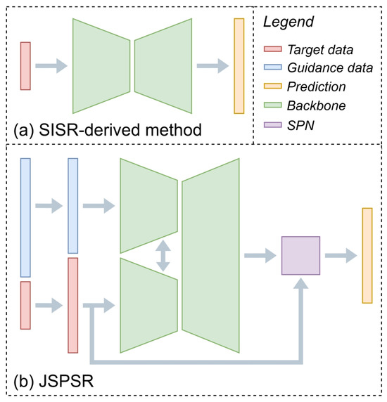
Figure 1.
Outline of SISR-derived method and JSPSR. (a) SISR-derived method predicts SR output from target data. (b) JSPSR predicts SR output based on target data and fused guidance features in the SPN module.
In the following sections, an overview of the dataset developed for validating methods (Section 3.1) and the data scaling used (Section 3.2) is provided, followed by details of the JSPSR network design in Section 3.3. Additional data processing details are included in Appendix A.1.
3.1. Dataset Development
Due to the lack of benchmark datasets for real-world DEM SR tasks, we developed a dataset to conduct experiments and compare the results of different DEM SR methods. We determined that an ideal real-world DEM SR dataset should contain the following components: high-resolution DTM samples as the ground truth, high-resolution remote sensing image samples as the guidance data, low-resolution DSM samples as the target data of SR methods, other DTM samples (existing state-of-the-art dataset is preferred) as the comparison reference for the method performance, and at least one kind of land-surface information, such as land cover masks, land use masks, canopy height data, building footprints and street maps, as the auxiliary guidance samples. All the source data should be produced in similar periods and be publicly accessible. Following the above principles, considering the location, date and quality [6], we selected (1) the Copernicus GLO-30 DEM (COP30) dataset [12] as the low-resolution DSM source, (2) the Forest And Buildings removed Copernicus DEM (FABDEM) dataset [13] and FathomDEM dataset [14] as the comparison reference DTM source, (3) the HighResCanopyHeight dataset [58] as the Canopy Height Map (CHM) source, and (4) the GRSS Data Fusion Contest 2022 (DFC2022 or grss_dfc_2022) dataset [59] as the high-resolution image, DTM and land use mask sources, to build a dataset for real-world DEM SR problems, denoted here as DFC30 (DFC2022 + FABDEM/FathomDEM + COP30, low-resolution at ∼30 m). We note that while the pixel size of GLO-30 is 30 m, and the actual spatial resolution is unknown, it is derived from 0.4 arcsecond (∼12 m) TanDEM-X data [60].
Table 1 lists DFC30 components information.

Table 1.
DFC30 dataset components information.
Among the DFC30 dataset components, the DFC2022 dataset was developed based on the MiniFrance dataset [61], which defined a 1 km2 geographic bounding box for each sample. The sources of images, land use masks, and DTMs for the DFC2022 dataset are the BD ORTHO dataset [62], the UrbanAtlas 2012 dataset [63], and the IGN RGE ALTI dataset [64], respectively. DTMs of the DFC2022 dataset were derived from airborne LiDAR or correlation of aerial images at a resolution of 1 m, with a vertical accuracy of ∼0.2 m in flood or coastal areas [64]. The DFC2022 dataset comprises 3981 valid samples, each covering an area of 1 km2 of land within the selected sixteen regions in France, with a resolution of up to 0.5 m. The DFC2022 dataset covers around 4000 km2 in total, including urban and countryside scenes: residential areas, industrial/commercial zones, fields, forests, sea-shore, and low mountains. Based on the DFC2022 dataset sample boundary, we supplemented the samples with the same boundary from the COP30, FABDEM, FathomDEM, and HighResCanopyHeight datasets to constitute the DFC30 dataset. Figure 2 illustrates the sample locations and data distributions of the DFC30 dataset with an example region and an example sample.
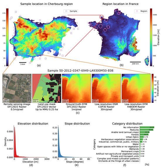
Figure 2.
DFC30 dataset sample location, example, and distribution. All 3981 samples in the DFC30 dataset are located in selected sixteen regions of France. Each sample contains a high-resolution image, a high-resolution land use mask, a high-resolution CHM, a high-resolution DTM, a low-resolution DSM and two low-resolution DTMs. (a) The location of samples in the example region (Cherbourg); (b) the locations of 16 regions; (c) an example sample for training; (d) the density distribution by elevation; (e) the density distribution by slope; (f) the category distribution by percentage.
To improve data transformation efficiency during training, we preprocessed the DFC30 dataset by resampling the data to the target resolution in advance. There are several constraints in determining an appropriate target resolution:
- Guidance information degradation: Remote sensing images (or other auxiliary spatial data) lose detail at lower resolutions. Considering road width, tree canopy radius, and residential property size, an 8 m resolution is an appropriate threshold. If the resolution is coarser than 8 m, ground features (e.g., narrow roads, individual trees, and small houses) may be lost during downsampling to the target resolution from high-resolution data.
- Network input limitation: JSPSR only allows input tensors with shapes that are multiples of 8 (e.g., 128 × 128, 144 × 144, etc.). The input shape of 128 × 128 pixels is the minimal adequate size for feature extraction in networks, equivalent to ∼8 m resolution.
- Computational efficiency: training with very high resolution (e.g., 1 m resolution) data is expensive due to the vast amount of data for training, which will slow the experiment progress.
Therefore, this work selected resolutions of 8 m and 3 m as the target resolutions for experiments.
The DFC30 dataset was preprocessed to 8 m and 3 m resolution samples for network training and evaluation, denoted as DFC30-8m and DFC30-3m , respectively. More details of data processing are described in Appendix A.1.
3.2. Elevation Data Scaling
As the density plot in Figure 2d shows, the elevation distribution is close to the power law distribution, which is highly skewed towards zero elevation in an extremely narrow value range compared to the total value range, which would lead to inferior network performance [65]. Therefore, we scaled the raw elevation data to mitigate the adverse effects of data skew by converting the data distribution closer to a normal distribution using the process described here.
Assuming is the elevation of a low-resolution DEM sample i, is its min–max scaling result, and a vanilla min–max data scale can be defined by the following:
where and are pre-defined minimum and maximum scale range parameters, respectively. The is equal to or smaller than the lowest elevation in all DEMs in the dataset, and is equal to or greater than the highest elevation in all DEMs in the dataset. To simplify the illustration, we assume the overall elevation range of the DEMs is (−100, 2900), denoted as and , and the elevation difference range (i.e., highest elevation subtract lowest elevation) in each DEM sample of all DEMs in the dataset is a (−1, 399) range, denoted as and .
Using a sample from the Marseille–Martigues region as an example (ID: 13-2014 0908-6289 LA93-0M50-E080), Figure 3a shows the three-dimensional visualisation of the min–max scaled Y channel of the remote sensing image, which has a 0.2 to 0.8 data range. For comparison, Figure 3b is the min–max scaled DEM in the range (−100, 2900), with a 0.1 to 0.2 data range, which is much narrower than the RGB image value range and highly skewed towards zero. Considering the fact that the features (such as slope and aspect) of a DEM will remain if changing the geoid, it will not affect the feature extraction of the networks if we shift a DEM to a 0-based relative elevation DEM, denoted as , by subtracting the lowest elevation of the DEM:
Relative elevation helps reduce data skew by providing a smaller min–max range for scale. Each DEM can then be min–max scaled to a 0-based relative elevation, denoted as , using the following:
where the and are pre-defined minimum and maximum scale parameters of relative elevation in the whole DEMs, specifically (−1, 399) as previous assumption, improved over seven times regarding the value range (i.e., from (−100, 2900) to (−1, 399)), as Figure 3c shows. However, although the data distribution becomes more expansive, it remains skewed towards 0.
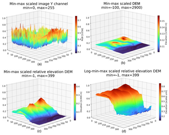
Figure 3.
Data scale results of a sample: (a) min–max scaled image Y channel, min and max values are the 8-bit integer range; (b) min–max scaled DEM produced using Equation (1), min and max values are elevation min and max values of the whole dataset (−100 and 2900 in this case); (c) min–max scaled relative elevation DEM, min and max values are the 0-based relative elevation min and max values of the whole dataset (−1 and 399 in this case); (d) log-min–max scaled relative elevation DEM, min and max values are the same with (c). The log-min–max scale on the relative elevations (d) significantly extended the data distribution range and amplified the low-elevation details, which improves performance in low-relief samples but may undermine feature extraction in higher-elevation pixels.
Since the logarithmic scale generally reduces power law distribution, we applied a logarithmic operation to both the numerator and denominator in the relative elevation min–max scale from Equation (3), to provide the log-min–max scaled elevation, denoted as :
As shown in Figure 3d, the distribution of log-min–max scaled relative elevation DEM is less skewed and has a wider data distribution.
Figure 4 shows the distributions of the vanilla min–max scaled DEMs (Equation (1)) and the log-min–max scaled relative elevation DEMs (Equation (4)). Although the log-min–max scaled relative elevation DEM data distribution (Figure 4b) is still skewed to a particular value to a degree due to the negative elevation outliers, it mitigates the impact of the highly skewed data and, hence, is superior to the vanilla min–max scaled data distribution (Figure 4a).
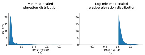
Figure 4.
Scaled to [0, 1] elevation of different method: (a) min–max scaled elevation distribution, , obtained using Equation (1), and (b) log-min–max scaled relative elevation distribution, , obtained using Equation (4). The distribution of (b) is less skewed to 0 than that of (a), which benefits the performance of networks.
3.3. Joint Spatial Propagation Super-Resolution Networks Design
Compared to SISR methods for DEM SR that only use low-resolution DEMs as input data, the proposed JSPSRs utilise low-resolution DEMs and guidance data (with or without auxiliary guidance data), which enables the networks to extract and leverage more features from input data for regression. However, the guidance data raise challenges regarding multi-modal feature fusion [66]. Therefore, fusing data with different modalities effectively and efficiently is the primary concern for the backbone of the JSPSR networks. Furthermore, unlike popular datasets, such as DIV2k [67], which uses synthetic low-resolution images, or KITTI [68], which captures point clouds and RGB images simultaneously in the exact location, the target data (i.e., low-resolution derived DSMs), guidance data, and ground truth (i.e., high-resolution derived DTMs) are entirely independent. That means that the same coordinate pixels of different components in a sample may not necessarily be precisely matched due to time differences and system biases, which requires our network to learn features and predict output non-locally. Thus, we designed networks focusing on addressing the above two issues.
Our solution for multi-modal feature fusion is Guided Image Filtering (GIF) (Section 3.3.1). For pixel mismatch, our solution is non-local SPN methodologies (Section 3.3.2). The outline of the proposed approach is illustrated in Figure 1, which shows the coarse architecture. More details are depicted in Figure 5, which comprises a U-Net [69] structure with multi-branch encoders and a single-branch decoder, and a SPN module.
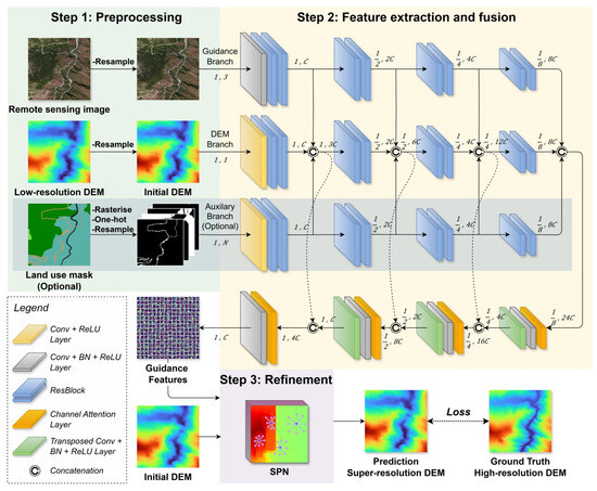
Figure 5.
The architecture of JSPSR and the training workflow. The preprocessing (Step 1, described in Section 3.1) upsamples the low-resolution DSM to the target resolution as the initial DEM and sends the initial DEM with guidance image and optional auxiliary guidance data (land use mask in this case) to the corresponding branch of the backbone for multi-modal feature extraction and fusion (Step 2, described in Section 3.3.1). The refinement process (Step 3, described in Section 3.3.2) utilises a non-local SPN to tune the initial DEM based on guidance features extracted from the backbone and to estimate the SR DEM.
3.3.1. Guided Image Filtering
Li et al. [46] proposed the deep joint image filtering network, which sends guidance input and target input in two branches of convolutional layers separately, then concatenates the output of the two branches and extracts features again through convolutional layers to obtain the feature-fused output. This structure efficiently fuses multi-modal features (e.g., [43,44,57]). There are two main strategies for multi-modal feature fusion: early fusion and late fusion. Methods that adopt early fusion depend on the strong feature extraction ability of the encoder to fuse multi-modal features, which leads to the encoder being computationally intensive (e.g., PENet [47], with 132 million parameters, and CompletionFormer [49], with 83.5 million parameters). In contrast, methods that adopt late fusion have a dedicated branch to extract features for each input modality, making the network more efficient when the number of branches is small. However, the parameter size increases rapidly with the number of branches using later fusion. Considering SR is a low-level computer vision task that should ideally not involve high computational costs, we selected the late fusion mode referring to the guided image filtering theory, as shown in Figure 5 (Step 2). The total parameter size of our networks with a two-branch encoder is 29.16 million, and with a three-branch encoder is 43.87 million.
3.3.2. Spatial Propagation Network
The Spatial Propagation Network (SPN) was initially designed to alleviate the depth mixing problem by learning affinity from guidance features [50]. With the enhancement of the deformable convolution networks [70], non-local SPN variants have been proposed (e.g., [44,49,53,57]), which have found that the non-local SPN improves the depth accuracy on the edge of objects. This attribute could be helpful for DEM SR since our DEMs are relatively “flat” in most samples (slope smaller than 10°), which means “blur” in the RGB image perspective. During training, the SPN collects the affinity of eight neighbour pixels of each pixel to assist elevation prediction and then learns the offset (x and y directions) and weight (or confidence in some studies [49,53]) in the backpropagation stage, as shown in Figure 6. After appropriate training, the learnt SPN offset and weight can significantly contribute to the elevation prediction performance.
Figure 6.
Example of non-local spatial propagation: three pixels (yellow) that select their most similar neighbour pixels (purple) in eight different directions to assist elevation prediction while ignoring low-similarity neighbours. This approach alleviates errors caused by pixel mismatches between the guidance image, the low-resolution derived DEM, and the high-resolution derived ground truth, as the SPN learns the similarity during training, allowing for pixel offsets in elevation prediction.
We built on DKN [57] and LRRU [44] to implement the non-local SPN refinement module as shown in Figure 7. The refinement module reconstructs input initial DEMs using guidance features in a deformable convolutional layer. It generates deformable convolutional kernel affinity weight parameters and sampling offset parameters for each pixel to fulfil non-local learning. It then learns the parameters during training and fine-tunes the initial DEM elevations. The refinement module has a residual connection between the initial DEM and the final output to augment high-frequency information and suppress noise. Therefore, it intrinsically learns the residual between the prediction and the ground truth. The main differences between our refinement module and the previous SPN refinement modules are:
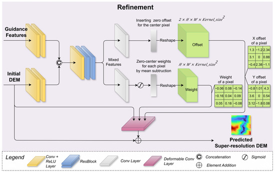
Figure 7.
The refinement module structure. It first generates offset prediction and weight prediction for each pixel in the initial DEM based on mixed features. Then, it utilises a modulated deformable convolutional layer to sample neighbouring pixels based on the offset and weight to predict the SR DEM in a non-local style.
- Less computing cost: our refinement module runs once per batch during training and inference, while the previous works need to run iterations per batch;
- Optimised high-frequency information: our refinement module directly uses initial DEMs as one of the inputs, and it does not contain a batch normalisation layer, which gains access to more high-frequency information to contribute to the DEM reconstruction quality.
3.3.3. Implementation
We selected Python 3.10 and PyTorch 23.05 [71] to implement our framework for training and evaluating, including data augmentation, data transformer, data loader, network, loss function, metrics, training procedure, and evaluation procedure.
As shown in Figure 5, initially, low-resolution DEMs are interpolated to the target resolution as the initial DEM, similar to SRCNN [19]. Each type of input data (i.e., initial DEM, guidance image, and auxiliary guidance data) of the networks has its feature extractor branch (encoder). Among branches, they share features with the DEM branch by concatenating. With this structure, the three ResNetBlock [72] layers (two parallel before and one after the concatenating operation) perform guided image filtering to optimise fusing the different modality features. Then, the transposed convolutional layers in the decoder fuse and upsample the features from the encoders to create the guidance features for refinement. A channel attention layer [73] is located before each transposed convolutional layer to emphasise significant channels. Ultimately, the refinement module fuses features from guidance features and initial DEMs through guided image filtering, creating mixed features, and then generates weight and offset parameters for the deformable layer to predict SR DEM residuals. In brief, the network has a U-Net encoder-decoder structure with multiple branch encoders for feature extraction and multi-modal fusion, a single decoder for feature fusion that serves as a feature pyramid, and a refinement module for reconstructing the final predicted SR DEMs.
We adopted the following loss functions to supervise the network training progress: Mean Absolute Error (MAE), denoted as , Mean Square Error (MSE), , and edge loss, , to evaluate the pixel-wise distance between the prediction , where is the elevation of the prediction i, and the ground truth , where is the elevation of the ground truth DEM sample i. The loss functions are defined as follows:
where denotes the result of the Sobel operator for edge detection. For the combined loss function, , indicates the weight of a loss. We set , , and for optimum performance.
To evaluate the quality of predictions, we defined elevation error as the pixel-wise deviation between a DEM and its corresponding ground truth. We selected the Root Mean Square Error (RMSE), elevation median error (Mdn.), Normalised Median Absolute Deviation (NMAD), absolute deviation at the 95% percentile (LE95), and Peak Signal-to-Noise Ratio (PSNR) as metrics. These metrics are defined by the following:
where in Equations (10) and (12) means the percentile value at x position in set s. in Equation (13) denotes the pre-defined maximum of elevation, as mentioned in Section 3.2.
This metric combination comprehensively considers the accuracy, error distribution, and sensitivity to outliers. In addition, it facilitates comparison with the existing literature. Among the metrics, RMSE is the most commonly used and significant criterion. However, RMSE assumes the errors follow a normal distribution with insignificant outliers, which is infrequent in DEM studies [74]. In common with previous DEM studies [6,74,75,76], we supplemented RMSE with three robust metrics (Mdn., NMAD, and LE95) to describe the properties of the error distribution in cases where elevation errors are not normally distributed. Additionally, we utilised PSNR to measure the difference between two images, serving as a metric for evaluating image reconstruction quality. However, PSNR uses a pre-defined maximum parameter (), which may vary in different datasets, methods or tasks, causing the PSNR not to be suitable for direct comparison between other studies if is different.
Specific details of the metric calculation and dataset training/test split are provided in Appendix A.2 and Appendix A.3, respectively.
3.4. Other Methods for Comparison
We selected three other methods for comparison with JSPSR on the DFC30 dataset: EDSR [30], CompletionFormer [49], and LRRU [44]. EDSR is a classic method for SISR problems and has been widely adopted as a baseline in many studies. Unlike the original implementation, our version of EDSR omitted upsampling layers because we preprocessed input data to the target resolution. CompletionFormer and LRRU were state-of-the-art methods for depth completion. Both employ non-local SPN for refinement. However, CompletionFormer uses an early fusion mode, whereas LRRU uses a late fusion mode. Among these methods, EDSR and CompletionFormer have single-branch architectures that can accept arbitrary multi-modal inputs through concatenation. In contrast, LRRU has a two-branch encoder structure, limiting it to two separate input sources. Since JSPSR can adapt its encoder structure to two or more input branches, we denote these variants as JSPSR2b (2b means two-branch) and JSPSR3b (3b means three-branch) for clarity. The attributes of all compared methods are summarised in Table 2.
Table 2.
The attributes of models for comparison.
Due to the differences in size and resolution, it is challenging to directly compare the metrics between low-resolution DEMs and ground truth DEMs. Therefore, we used bicubic upsampling of low-resolution DSMs (COP30) and low-resolution DTMs (FABDEM and FathomDEM) to the target resolution, then calculated metrics between them and ground truth as baselines to compare with other methods. These are denoted as BaseCOP30, BaseFABDEM, and BaseFathomDEM.
4. Results
Based on the datasets, networks, loss function, metrics, and procedures described above, we conducted experiments on the DFC30-8m and DFC30-3m datasets for the 30 m to 8 m and 30 m to 3 m SR tasks, respectively. The following sections will report the experimental setup and results, including comparison studies, ablation studies, and visualisations.
4.1. Experimental Setup
We deployed JSPSR and other methods for comparison with the DFC30 dataset to generate ground elevation DTMs with target spatial resolutions of 8 m and 3 m. The training input data used were from one of the preprocessed datasets (i.e., DFC30-8m or DFC30-3m, as illustrated in Section 3.1), consisting of low-resolution derived DSMs, high-resolution derived images, high-resolution derived land masks, and high-resolution derived CHM. The ground truth data were the high-resolution derived DTMs.
The transformer of our framework first applied 0-based elevation shifting and log-min–max scaling (Section 3.2) to optimise data distribution, then executed random flip augmentation horizontally and vertically for data augmentation. The 4D batch size (Batch × Channel × Width × Height) is configurable: Batch is set from 17 to 70 based on the maximum GPU memory capacity, Channel automatically fits the input data channel number, and Width × Height is set to pixels by default. For DFC30-8m, the transformer will not crop it, since each sample is already in a pixel size. For DFC30-3m, the transformer crops each sample from pixels to nine patches of pixels in a tiling style, completely covering a sample with overlapped pixels. Thus, the prediction of a DFC30-3m sample consisted of nine overlapping predicted tiles. We applied a smooth linear weighting to the overlapped pixels among the nine tiles to generate a seamless 3 m DTM prediction. When the transformer converts DEMs into input tensors, it preserves all spatial information (including CRS and coordinates), which are subsequently used to transform the predicted tensors back into DEM raster files as the final SR predictions.
We adopted AdamW [77] as the optimiser with of 0.9, of 0.999, weight decay of , and a step-decay learning rate scheduler starting from with decay ratio 0.5 and epoch step 100. The early stop method was applied during the default 300 training epochs. The computing platform consisted of a Linux workstation equipped with an Nvidia GeForce RTX 4090 GPU. A Docker container was deployed to build and manage the software environment, which was pulled from the Nvidia NGC Catalogue (tag: pytorch:23.10-py3).
4.2. Experimental Results
A summary of the experimental results for method and data combination is presented in Table 3, which reports the overall RMSE results for each. JSPSR achieves the highest accuracy on both the 30 m to 8 m and 30 m to 3 m SR tasks, improving vertical accuracy (i.e., RMSE) by 71.74% and 71.1%, respectively, compared to BaseCOP30. Generally, methods that utilise auxiliary guidance data (i.e., land use masks or CHM) outperform models that rely solely on image guidance data, as the auxiliary guidance data can contribute to network regression, particularly for CompletionFormer, which significantly benefits from this additional information.
Table 3.
RMSE and change percentages of different methods on 30 m to 8 m and 30 m to 3 m SR tasks. Input data options are DEM, image, land use mask and canopy height map (CHM). The lower RMSE represents better performance. The value in the column represents the change percentage compared to the baseline values of BaseCOP30, BaseFABDEM, and BaseFathomDEM, respectively. The ↑ or ↓ indicates an increase or a decrease. The bold values highlight the best prediction performance for the task.
Figure 8 visualises the elevation error distribution and RMSE of the best result from different methods on the DFC30-8m dataset. The COP30 and its derived DEMs (i.e., FABDEM and FathomDEM) show a bias compared to the LiDAR-derived ground truth DEMs. All deep learning models corrected the bias and showed prediction error centred at 0. JSPSR has a narrower error distribution and obtains better performance.
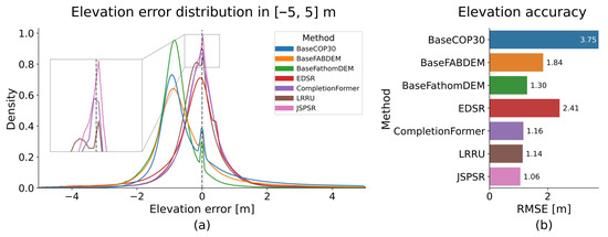
Figure 8.
Comparison between baselines and the best prediction of methods. (a) Elevation error distribution between −5 m and 5 m. (b) Elevation vertical accuracy (30 m to 8 m task, best performance of a method and guidance data combination).
The detailed results of all metrics used (detailed in Section 3.3.3) are reported in Table 4. JSPSR achieves the best or second-best value in all metrics, indicating that its prediction has optimal vertical accuracy, statistical distribution, and image reconstruction quality. Among the compared methods, EDSR achieves the lowest performance because SISR-derived approaches estimate predictions based on low-level image features, such as textures extracted from input data, which are not rich in DEMs, especially in low-relief areas. Unlike SISR approaches, depth completion approaches are designed to fuse multi-modal data and utilise the rich features from guidance data (i.e., images or other spatial data) to estimate depth. Therefore, both depth completion methods, CompletionFormer and LRRU, significantly improve performance compared to approaches that only input DEMs. However, the dataset for depth completion problems is much larger and more complex than DEMs, leading to the depth completion networks generally containing massive neural network layers and multi-iterative refinement modules, such as GuideNet [43], PENet [47], RigNet [78], CompletionFormer [49], and LRRU [44], that may be unnecessary or adverse to DEM SR tasks due to overfitting. On the contrary, JSPSR achieved superior performance with relatively fewer network parameters and a one-shot refinement, thereby reducing the computing cost.
Table 4.
Metrics of different methods on 30 m to 8 m and 30 m to 3 m SR tasks. Input data options are DEM, image, land use mask and canopy height map (CHM). The ↓, , and ↑ mean the lower, the lower absolute, and the higher value represents better performance for the metric, respectively. The red colour value is the best value of a metric in an SR task, while the blue is the second-best.
Beyond quantitatively comparing prediction performance, we evaluated inference time and GPU memory consumption to compare the computing cost among selected methods on the DFC30-8m dataset, as shown in Table 5. The input data resolution is 8 m, and the size is 128 × 128, with a batch size of one. PyTorch application programming interfaces (APIs) are utilised to measure the GPU inference time and memory costs precisely. We inferred all 799 test samples and calculated the average values (except for the first inference, which was affected by extra overhead from PyTorch). The experimental results indicate that JSPSR achieves the fastest inference speed and moderate memory consumption on GPUs. It is worth mentioning that our end-to-end DEM SR approach incurs an additional CPU computing cost for resampling low-resolution DEMs to the target resolution using GDAL [79], which typically takes less than 0.3 ms to resample a sample using GDAL on a 4 GHz CPU core.
Table 5.
Computing cost comparison of different methods on the DFC30-8m dataset. The inference sample size is 128 × 128, and the resolution is 8 m. GPU time and GPU memory usage are the average computing costs of inferring 798 test samples. The red colour value is the best in a column, while the blue is the second-best.
To visually compare the SR reconstruction quality, we selected two extreme scenarios for comparison: the most improved and the least improved cases using JSPSR. Figure 9 displays the most improved JSPSR prediction compared to BaseCOP30. In this case, the BaseCOP30 RMSE of this sample is 15.58 m, while the JSPSR prediction RMSE is 3.29 m, representing an improvement of 78.9%. EDSR and CompletionFormer appear underfit, which does not account for part of the canopy height. The predictions of LRRU and JSPSR acquire higher quality than those of other methods. However, the LRRU prediction displays signs of overfitting, as small stripes appear in pixels with very low relief.
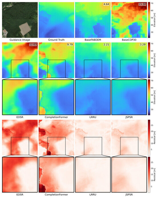
Figure 9.
Comparison among predictions of different methods in the case of the most improved prediction with JSPSR compared to BaseCOP30, displayed in the format of elevations and residuals to the ground truth with partially enlarged details. The number in the top right corner is the RMSE of this sample/prediction. (30 m to 8 m SR task, image guidance only, sample ID: Lille 59-2012-0703-7040 LA93-0M50-E080).
On the other hand, Figure 10 displays the least improved JSPSR prediction compared to BaseCOP30. The RMSE of this BaseCOP30 sample is 2.75 m, while the JSPSR prediction RMSE is 3.39 m, increasing 23.3%. All the methods try to predict the depth of the ditch covered by vegetation. However, they all overestimate the depth of the ditch, leading to the raw input data achieving the best performance. It highlights that predicting elevation under vegetation is a challenge for all DEM SR methods in this context.
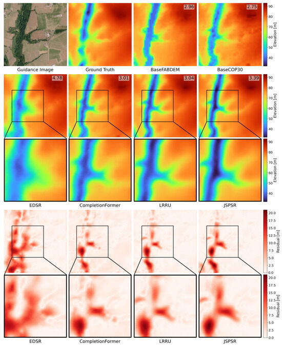
Figure 10.
Comparison among predictions of different methods in the case of the least improved prediction with JSPSR compared to BaseCOP30, displayed in the format of elevations and residuals to the ground truth with partially enlarged details. The number in the top right corner is the RMSE of this sample/prediction. (30 m to 8 m SR task, image guidance only, sample ID: Angers 49-2013-0415-6696 LA93-0M50-E080).
4.3. Ablation Studies
We conducted experiments on the DFC30-8m dataset to evaluate the effectiveness of the proposed method’s components, guidance data, and generalisation.
4.3.1. Effectiveness of Proposed Data Scale Method
Data preprocessing is a fundamental factor in determining the quality of training. Before the low-resolution DSM (COP30) is transformed to tensors for training, they are interpolated to the target resolution using the bicubic algorithm, augmented with random flips and then scaled to [0, 1] using a relative elevation log-min–max scale, as illustrated in Section 3.2. We conducted experiments to compare the effectiveness of the relative elevation log-min–max scale, as shown in Table 6. The RMSE decreased by 14.9% when guidance data consisted of images, and by 12.7% when guidance data consisted of images and land use masks, indicating that our relative elevation log-min–max scale method effectively improves network performance.
Table 6.
RMSE comparison between with and without relative elevation and log-min–max scale in 30 m to 8 m SR task (image guidance only). The ↓ means the lower value represents better performance.
4.3.2. Effectiveness of Guidance Data
The impact of different guidance data on JSPSR is reported in Table 7. We conducted experiments on EDSR and JSPSR to evaluate the significance of guidance data, including images, land-use masks, and CHMs. We also assessed JSPSR performance without image guidance, using only the land use mask or CHM auxiliary guidance. The experimental results confirm the significant enhancement of guidance images. With guidance images, EDSR performance significantly improved by over 30% compared to without guidance images. JSPSR also improved with guidance images compared to without guidance images.
Table 7.
RMSE of JSPSR on 30 m to 8 m and 30 m to 3 m SR task. Input data options are DEM, image, land use mask and canopy height maps (CHM). The ↓ means the lower value represents better performance.
Regarding the two types of auxiliary guidance data, their contributions are contingent upon specific conditions. Incorporating the guidance images, since CHM can be directly learnt from ground truth, the contribution of CHM is slightly less significant than that of land use masks, which contain more additional information than CHM. Without the guidance images, the networks appear less effective with auxiliary guidance land use masks than CHM.
4.3.3. Comparison of Data Fusion Operations for Guided Image Filtering (GIF)
JSPSR adopts the GIF method for feature extraction and multi-modal fusion. In general, there are three simple operations for fusing features between the encoder and decoder branches: addition, concatenation, and filtering. The addition and concatenation approaches are fundamental operations for binding features together. The addition operation adds different features element-wise, while the concatenation operation stacks different features in the channel dimension. The filtering approach uses convolutional kernel filters (e.g., LRRU [44]) or customised kernel filters (e.g., GuideNet [43]) to fuse features. Many other elaborate approaches for multi-modal data fusion have been proposed [80], but they are outside the scope of this work. We assessed the effectiveness of addition, concatenation, and convolutional kernel filtering, as shown in Table 8, which suggests that the concatenation approach achieves better performance under similar parameters and computational costs on the DFC30-8m dataset.
Table 8.
RMSE comparison among different fusion operations on DFC30-8m dataset. The ↓ means the lower value represents better performance.
4.3.4. Effectiveness of Refinement Module
The refinement module is a prominent component for depth completion approaches. It is also a significant difference between the proposed JSPSR and SISR-derived methods. Table 9 compares the metrics with or without the refinement module for EDSR and JSPSR on the DFC30-8m dataset. It reported that the refinement module improved network performance remarkably (up to 48.3% on RMSE), even though the network was an SISR method (EDSR), which was enhanced by 48% on RMSE with the guidance image and refinement module.
Table 9.
RMSE comparison with or without refinement module on DFC30-8m dataset. The ↓ means the lower value represents better performance.
4.3.5. Generalisation
Generalisation is a crucial ability to predict unseen data. The fixed train/test split in previous experiments cannot assess the generalisation of the proposed method. To evaluate model generalisation, we conducted experiments on different train/test splits using the k-fold cross-validation method, specifically setting each region as the test set and the rest of the fifteen regions as the training set. The results are reported in Table 10. Most regions achieved over 50% improvement compared to BaseCOP30, and over 20% improvement compared to BaseFABDEM and BaseFathomDEM. However, the two high slope regions (Nice and Marseille–Martinique) achieved underperforming results. A possible reason is that these are the only two regions (Nice and Marseille–Martinique) in the mountainous area of the DFC30 dataset, leading to the high-slope areas being under-fitted during training. Evidence is that the third high slope region (Clermont–Ferrand) achieved a 63.63% improvement compared to BaseCOP30, as the two mountainous regions are included in the training set, allowing the network to learn enough features of high slope samples, compared to learn from only one mountainous region. In general, the model generalisation of JSPSR is robust, except for high-slope regions due to the insufficiency of high-slope samples in the DFC30 dataset.
Table 10.
16-folder cross-validation on 30 m to 8 m SR task (image guidance only). The region name indicates that the region serves as the test set, and the remaining 15 regions are used as the training set. “COP.”, “FAB.”, and “Fat.” represent BaseCOP30, BaseFABDEM, and BaseFathomDEM, respectively. represents the metric change percentage compared to baselines. The ↑ or ↓ indicates an increase or a decrease. The value after ↑ or ↓ is the change percentage compared to baselines. The red values highlight the most improvement, while the blue values highlight the lowest.
4.4. Assessment of JSPSR Predictions by Topographic Context
The experimental results above validated the performance of the proposed method under various conditions. However, it does not take into account topographic attributes. In this section, we analyse the prediction of the proposed method in the topographic context.
4.4.1. Vertical Accuracy by Slope
Topographic slope is strongly influenced by DEM resolution due to the scale difference of a point under different resolutions [81]. Generally, lower elevation accuracy will be measured where an SR output has a higher slope. Thus, we assessed the RMSE based on different slope ranges (<5°, 5–10°, 10–25°, and >25°), as shown in Table 11, which indicated that accuracy decreased as the slope increased. However, JSPSR achieved superior accuracy across all slope ranges (except when the slope exceeded 25° on the 30 m to 8 m SR task), outperforming BaseCOP30 (an improvement of up to 73.2%), BaseFABDEM (an improvement of up to 43.65%), and BaseFathomDEM (an improvement of up to 17.72%), particularly in low-relief areas.
Table 11.
RMSE comparison under different slope ranges on 30 m to 8 m and 30 m to 3 m SR tasks. represents prediction RMSE change percentage compared to BaseCOP30, BaseFABDEM, and BaseFathomDEM, respectively. The ↓ or ↑ indicates an increase or decrease compared to the corresponding baseline.
One of the reasons for lower performance in the higher slope range is that the slope distribution of the DEM30 dataset is highly skewed. The pixel percentage of each slope range is approximately 93% (<5°), 5% (5–10°), 1.6% (10–25°), and 0.1% (>25°), leading to potential under-fitting when pixel slopes become higher.
4.4.2. Vertical Accuracy by Land Use Mask Categories
Land use masks present the various land use or land cover categories, including water, urban fabric, pastures, forests, and others. They affect prediction accuracy due to the inclusion of semantic information from classification and segmentation. This semantic information may facilitate feature extraction and fusion when different data (e.g., images, DEMs, and land use masks) are pixel-wise matched. However, it may introduce noise if they are widely mismatched, which can impair prediction performance. Since the land mask classes are highly unbalanced, as shown in Table 12 (pixel percentage column), the RMSE of each category does not reveal the correlations between JSPSR and land use mask categories. However, by comparing the results with and without the land use mask guidance, we determined which category benefits the most (or least) from the land use mask guidance. Additionally, comparing predictions and baselines by land use mask classes helped to evaluate the network’s performance and limitations. Figure 11 demonstrates elevation profiles from several samples to show the detailed elevation compared with baselines. Although several elevation profiles do not have a statistical meaning, it is a straightforward way to reveal whether a method is effective.
Table 12.
RMSE comparison by land use mask classes on 30 m to 8 m SR task. “COP.”, “FAB.”, and “Fat.” represent BaseCOP30, BaseFABDEM, and BaseFathomDEM, respectively. “W/O.” and “W.” mean without the land use mask guidance and with the land use mask guidance. The represents RMSE change percentage compared to baselines and W/O. The ↓ or ↑ indicates an increase or decrease. The red values highlight the most improvement, while the blue values highlight the lowest.
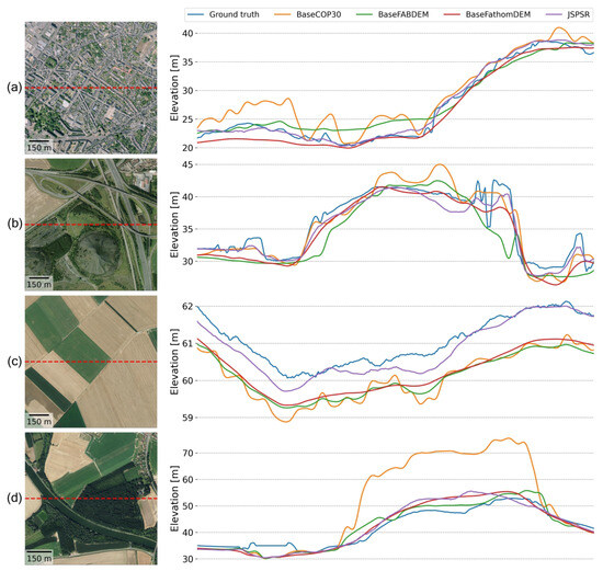
Figure 11.
Elevation profiles by land use mask classes. The red-dashed lines are elevation cross-section projections on the remote sensing images. (a) Class 1 (urban fabric). (b) Class 2 (industrial, commercial, public, military, private, and transport units). (c) Class 5 (arable land (annual crops)). (d) Class 10 (forests) and 14 (water). (30 m to 3 m SR task, image + land use mask guidance).
Based on the statistics in Table 12, the RMSE of SR predictions with land use mask guidance was slightly better than the RMSE without land use mask in general. Specifically, the land use mask guidance contributed the most to class 11 (herbaceous vegetation associations), where the RMSE improved by 16.43% compared to the same condition without land use mask guidance. In contrast, the guidance data reduced network performance by 10.78% in class 6 (Permanent crops). Compared to the baselines, the most significant difference is the FathomDEM RMSE of class 10 (Forests), which is superior to all other categories because FathomDEM utilises canopy height for training and dramatically improved canopy height prediction performance. All other categories basically follow the rule that a lower slope performs better, except for the forest category, which contains relatively more high-slope pixels, yet achieves the best performance.
The statistics may imply that (i) land use mask guidance contributed less when the class segmentation boundaries are less accurate in higher slope areas; (ii) land use mask guidance were helpful when a class had apparent visual features (e.g., buildings, wetlands and forests); (iii) land use mask guidance may have decreased prediction performance when a class was visually ambiguous with other classes (e.g., class 11 herbaceous vegetation may look similar with class 5 agricultural vegetation); and (iiii) the influence of slope on performance is more significant than that of classes.
4.4.3. Vertical Accuracy for DSM to DTM
If the SR DEMs are downsampled back to the original low resolution, the results are equivalent to those of DSM-to-DTM processing (i.e., correction of errors without SR). To facilitate direct comparison with other datasets, we resampled the prediction SR DEMs from 8 m and 3 m to 30 m resolution, creating DTMs with the exact grid spacing as the input low-resolution DEMs (∼23.985 m). These DTMs can be used as DEMs with trees and buildings removed, which are functionally similar to FABDEM and FathomDEM. To maximise the use of predictions, we reprojected the original COP30, FABDEM and FathomDEM samples from EPSG:4326 to EPSG:2154. The quantitative comparison of elevation accuracy is reported in Table 13, indicating that our method outperforms COP30, FABDEM, and FathomDEM by over 70%, 40% and 17%, respectively, in terms of RMSE for DSM-to-DTM tasks on the DFC30 datasets.
Table 13.
Accuracy comparison among COP30, FABDEM, FathomDEM, and SR prediction at 30 m resolution. The subscript “2154” indicates that it reprojects from EPSG:4326 to EPSG:2154. represents RMSE change percentage compared to baselines. The ↓ indicates a decrease.
5. Discussion
The most significant benefit of JSPSR over SISR-derived methods, such as EDSR, is its fundamental approach to the problem. EDSR treats a DEM as a standard image, aiming to synthesise high-frequency texture details [30]. However, DEMs, especially high-resolution DEMs in low-relief areas, are devoid of such textures, leading to EDSR underperformance (RMSE of ∼2.4 m). In contrast, JSPSR re-frames the task as a height correction problem in three-dimensional space. By leveraging guidance from imagery and other spatial data, it learns to correct elevations based on information from different modalities (e.g., image features and semantic features) rather than merely elevation. This results in a 56% improvement in RMSE over EDSR.
In addition, the benefit of the tailored data scaling is worth emphasising. Severe skew in elevation values towards zero is characteristic of real-world, high-resolution DEMs in low-relief areas and hinders neural network performance [65]. The proposed relative elevation log-min–max scaling method was explicitly designed to address this distribution flaw. The ablation study confirmed that this approach alone provided a ∼15% boost in RMSE. This improvement is applied universally across all models under examination, including the other two compared models (i.e., DepthCompletion and LRRU).
However, the model’s performance in high-relief areas reveals a key limitation: its dependence on the topographic diversity of the training data. Future work will focus on incorporating more varied and balanced terrain into the training process and exploring the integration of additional data modalities, such as multispectral imagery and ICESat-2 (Ice, Cloud, and Land Elevation Satellite-2) data, to improve generalisation and overcome persistent challenges like accurately estimating ground elevation under dense vegetation.
Due to its multi-modal fusion capabilities, JSPSR has considerable potential for application in other geospatial tasks, such as remote sensing images of trees (or buildings, riverbanks, water, etc.) segmentation. Existing segmentation methods mainly utilise a single input data during training of networks (excluding post-processing, which may involve other data), such as images or point clouds, to predict semantic boundaries. They either lack height information or vision information, which limits the network performance. JSPSR can simultaneously join two or more modalities to predict segmentation, thereby potentially achieving superior performance. Moreover, JSPSR strikes an exceptional balance between performance, parameter efficiency, and inference speed. These advantages open new possibilities for large-scale hydrological modelling, flood risk assessment, and environmental monitoring, particularly for researchers and organisations operating with limited resources. Further research is required to test JSPSR for additional locations and its implications for hydrological model accuracy.
While commercial high-resolution DEMs from corporations like Airbus (WorldDEM) or Maxar (Precision3D) exist, this study addresses a critical problem: the urgent need for high-quality, open-access, and globally consistent bare-earth elevation data. The significance of the JSPSR method lies not in its ability to compete with commercial products in terms of absolute accuracy for a specific locale, but rather in offering a viable, scalable, and democratising alternative for applications where commercial data is impractical. It provides an option to a future where anyone, anywhere, can access high-resolution bare-earth elevation data without prohibitive cost, licensing restrictions, or concerns about data consistency, as called for by Schumann and Bates [17]. As outlined by Winsemius et al. [82] in their response, such a DEM would find uses beyond flood hazard assessment, including in morphology, cadastral digitization and landslide predictions. Winsemius et al. [82] further call for such efforts to be concentrated in areas which may benefit most, especially developing countries with no local resources available to obtain or produce a high-resolution, high-accuracy DEM, particularly given the disproportionally high exposure of poor people to floods and droughts [83]. Our JSPSR method is able to achieve improved accuracy and spatial resolution at lower computational cost, from widely available high resolution imagery alongside global elevation data, and may be further improved through the inclusion of additional guidance data.
6. Conclusions
This study successfully introduced and validated the Joint Spatial Propagation Super-Resolution networks (JSPSRs), a novel deep learning framework that addresses the critical challenge of generating high-resolution, high-accuracy bare-earth DEMs from globally available, low-resolution DSMs. In addition, it developed a ready-to-analyse dataset for real-world DEM SR problems based on publicly accessible datasets in low-relief areas. By integrating principles from depth completion, specifically Guided Image Filtering (GIF) and non-local Spatial Propagation Networks (SPNs), and the relative elevation log-min–max scaling, JSPSR demonstrates a significant advancement over existing Single Image Super-Resolution (SISR) methods for real-world DEM enhancement. The experimental results suggest that JSPSR outperforms the investigated interpolation, SISR and depth completion methods in real-world DEM SR tasks. By learning from the guidance data, our method improved accuracy (RMSE) by 71.74% and reconstruction quality (PSNR) by 22.9% on the 30 m to 8 m resolution task compared to Bicubic interpolation. Compared to EDSR in the same task, it decreases RMSE by 56.03% and increases PSNR by 13.8%. Our method may have the potential to be applied to other elevation-related tasks. For DSM-to-DTM problems, our method achieved a 72.02% accuracy improvement (RMSE) at the 30 m resolution compared to COP30, outperforming FathomDEM by 17.66%. If this improvement can be replicated for other locations, it would enable the development of an accurate, global, low-cost, high-resolution bare-earth elevation model.
Author Contributions
Conceptualization, X.C. and M.D.W.; methodology, X.C.; software, X.C.; validation, X.C. and M.D.W.; formal analysis, X.C.; resources, M.D.W.; data curation, X.C.; writing—original draft preparation, X.C. and M.D.W.; writing—review and editing, M.D.W.; visualization, X.C.; supervision, M.D.W.; funding acquisition, M.D.W. All authors have read and agreed to the published version of the manuscript.
Funding
This research received no external funding.
Data Availability Statement
All the datasets used for training and evaluating networks here are freely available online: DFC30, DFC30-8m and DFC30-3m: https://zenodo.org/records/10937848 (accessed on 26 October 2025), DFC2022: https://ieee-dataport.org/competitions/data-fusion-contest-2022-dfc2022 (accessed on 10 August 2024), Urban Atlas 2012: https://land.copernicus.eu/en/products/urban-atlas/urban-atlas-2012 (accessed on 10 August 2024), COP30: https://portal.opentopography.org/raster?opentopoID=OTSDEM.032021.4326.3 (accessed on 10 August 2024), FABDEM: http://data.bris.ac.uk/data/dataset/s5hqmjcdj8yo2ibzi9b4ew3sn (accessed on 10 August 2024), FathomDEM: https://zenodo.org/records/14511570 (accessed on 28 January 2025) and HighResCanopyHeight: https://registry.opendata.aws/dataforgood-fb-forests (accessed on 28 January 2025).
Acknowledgments
We would like to thank Maria Vega Corredor for support in project administration and for reviewing the original manuscript, and three anonymous reviewers for their comments which helped to improve the clarity of the manuscript.
Conflicts of Interest
The authors declare no conflicts of interest.
Appendix A. Supplementary Methods
Appendix A.1. Data Assembly
Figure A1 summarises processes from source data to training tensors. The DFC2022 dataset provides land-use mask data for two regions, derived from the Urban Atlas 2012 dataset. For the remaining fourteen regions, we supplemented the land use masks with those from the Urban Atlas 2012 dataset. To avoid class mixing (multi-class pixels) when rasterising and resampling the land use masks from vector to raster, we converted the original vector data to one-hot multi-channel raster data, where each class has a dedicated channel, allowing a pixel to belong to different classes simultaneously (process 1 in Figure A1). We dropped the test partition of the DFC2022 dataset because it lacks georeference information. Since the Urban Atlas 2012 dataset covers smaller areas than images and DEMs, pixels excluded from the Urban Atlas 2012 dataset coverage were categorised as the “No information” class. In addition, for the consistency and integrity of raster data, we filled no-data pixels (mainly water areas) in high-resolution DTMs using COP30 corresponding pixels (process 2 in Figure A1), ensuring all DTM pixels were valid for model training and testing. In addition, all samples were transformed to a Coordinate Reference System (CRS) of EPSG:2154 (Lambert-93/RGF93 v1—France) (process 3 in Figure A1), the same as the DFC2022 dataset, to maximise the use of the high-resolution data.

Figure A1.
Data assembling and processing workflow. The MiniFrance dataset [61] first defined the geospatial boundary of samples and clipped samples from the remote sensing image dataset BD ORTHO [62] and the land use mask dataset UrbanAtlas 2012 [63]. Then, the DFC2022 dataset [59] complemented the DTM samples from the RGE ALTI dataset [64]. We further supplemented DSM samples from Copernicus DEM GLO-30 (COP30) [12], DTM samples from FABDEM [13] and FathomDEM [14], and Canopy Height Map (CHM) samples from HighResCanopyHeight dataset [58]. To accelerate tensor transformation, the DFC30 dataset was preprocessed, denoted as DFC30-8m dataset for the 30 m to 8 m SR task and the DFC30-3m dataset for the 30 m to 3 m SR task.

All samples were resampled to the target resolutions (8 m and 3 m resolution) using bicubic interpolation to either upsample the low-resolution DTMs and DSMs from ∼30 m resolution, or downsample the high-resolution DTMs, images, CHM, and land use masks from high resolutions, to the target resolutions. After this preprocessing, we generated an 8 m resolution dataset on pixels of 128 × 128 (including paddings) per sample (process 4 in Figure A1), with a total of ∼65.2 million pixels, denoted as DFC30-8m, and a 3 m resolution dataset on pixels of 334 × 334 per sample (process 5 in Figure A1), with a total of ∼444.1 million pixels, denoted as DFC30-3m. In brief, each of the DFC30-8m and DFC30-3m datasets contained 3981 samples with resolutions of 8 m and 3 m, respectively. Each sample included a low-resolution derived DSM, two low-resolution derived DTMs, a high-resolution derived DTM, a high-resolution derived RGB image, a high-resolution derived CHM and a high-resolution derived land use mask within each sample.
Appendix A.2. Metric Calculation Details
We calculated metrics iteratively on each batch, namely online mode, and once after an epoch, namely offline mode. Some metrics, such as RMSE and PSNR, differed between the online and offline calculation modes. Taking RMSE as an example, the online mode calculates and stores each batch’s RMSE during an evaluation procedure and then averages all the stored batch RMSEs as follows:
where M denotes the iteration number of each epoch, B denotes the batch size. Specifically, this work defines the evaluation batch size as 1. Thus, the online mode RMSE is the average of the RMSE for each prediction in this case.
The benefits of the online mode are that it reveals trends during an epoch’s training and has low memory consumption. In contrast, the offline mode calculates the RMSE for all predictions as described in Equation (9), which requires more memory space. However, online mode calculations can be unreliable for specific metrics under certain scenarios. For instance, if a batch sample is located entirely on the water, such as a lake or sea, the prediction could be identical or close to its corresponding ground truth. Under these circumstances, referring to Equation (13), the batch PSNR will be large due to the denominator (i.e., RMSE) being close to zero, resulting in an abnormally high online mode PSNR compared to the offline mode PSNR.
Since our DEM dataset contained samples from within a lake or sea, we adopted an offline mode as the calculation mode to provide a comprehensive description of the results. The metrics in this paper are offline mode values by default unless explicitly labelled as the online mode.
Appendix A.3. Training Set and Test Set Splitting
To maximise the use of data, we split the dataset into a training set (13 regions) and a test set (3 regions). The division was based on sample size, where the training set contains four times the number of samples in the test set (approximating an 80%/20% ratio). Figure A2 summarises the elevation, slope and land use class distributions for both sets. Specifically, the training set and test set sizes are 3182 and 799 for DFC30-8m, and 28,638 and 7191 for DFC30-3m. We maintained a fixed train/test split using a predefined list, while shuffling sample order in the dataloader during training.

Figure A2.
The training/test split details. (a) The region location of the training/test split; (b) the elevation distribution by boxplot for pixels in the train set and test set; (c) the slope distribution by boxplot for pixels in the train set and test set; (d) the category distribution by percentage of pixels in the train set and test set.

References
- Rocha, J.; Duarte, A.; Silva, M.; Fabres, S.; Vasques, J.; Revilla-Romero, B.; Quintela, A. The importance of high resolution digital elevation models for improved hydrological simulations of a mediterranean forested catchment. Remote Sens. 2020, 12, 3287. [Google Scholar] [CrossRef]
- Wechsler, S. Uncertainties associated with digital elevation models for hydrologic applications: A review. Hydrol. Earth Syst. Sci. 2007, 11, 1481–1500. [Google Scholar] [CrossRef]
- McClean, F.; Dawson, R.; Kilsby, C. Implications of using global digital elevation models for flood risk analysis in cities. Water Resour. Res. 2020, 56, e2020WR028241. [Google Scholar] [CrossRef]
- Nandam, V.; Patel, P. A framework to assess suitability of global digital elevation models for hydrodynamic modelling in data scarce regions. J. Hydrol. 2024, 630, 130654. [Google Scholar] [CrossRef]
- Zandsalimi, Z.; Feizabadi, S.; Yazdi, J.; Salehi Neyshabouri, S.A.A. Evaluating the Impact of Digital Elevation Models on Urban Flood Modeling: A Comprehensive Analysis of Flood Inundation, Hazard Mapping, and Damage Estimation. Water Resour. Manag. 2024, 38, 4243–4268. [Google Scholar] [CrossRef]
- Meadows, M.; Jones, S.; Reinke, K. Vertical accuracy assessment of freely available global DEMs (FABDEM, Copernicus DEM, NASADEM, AW3D30 and SRTM) in flood-prone environments. Int. J. Digit. Earth 2024, 17, 2308734. [Google Scholar] [CrossRef]
- Guth, P.L.; Van Niekerk, A.; Grohmann, C.H.; Muller, J.P.; Hawker, L.; Florinsky, I.V.; Gesch, D.; Reuter, H.I.; Herrera-Cruz, V.; Riazanoff, S.; et al. Digital elevation models: Terminology and definitions. Remote Sens. 2021, 13, 3581. [Google Scholar] [CrossRef]
- Dolloff, J.; Theiss, H.; Bollin, B. Assessment, specification, and validation of a geolocation system’s accuracy and predicted accuracy. Photogramm. Eng. Remote Sens. 2024, 90, 157–168. [Google Scholar] [CrossRef]
- Elaksher, A.; Ali, T.; Alharthy, A. A quantitative assessment of LiDAR data accuracy. Remote Sens. 2023, 15, 442. [Google Scholar] [CrossRef]
- Ho, Y.F.; Grohmann, C.H.; Lindsay, J.; Reuter, H.I.; Parente, L.; Witjes, M.; Hengl, T. GEDTM30: Global ensemble digital terrain model at 30 m and derived multiscale terrain variables. PeerJ 2025, 13, e19673. [Google Scholar] [CrossRef]
- Bielski, C.; López-Vázquez, C.; Grohmann, C.H.; Guth, P.L.; Hawker, L.; Gesch, D.; Trevisani, S.; Herrera-Cruz, V.; Riazanoff, S.; Corseaux, A.; et al. Novel approach for ranking dems: Copernicus DEM improves one arc second open global topography. IEEE Trans. Geosci. Remote Sens. 2024, 62, 4503922. [Google Scholar] [CrossRef]
- European Space Agency. Copernicus DEM—Global and European Digital Elevation Model; Copernicus Data Space Ecosystem: Zaventem, Belgium, 2022. [Google Scholar] [CrossRef]
- Hawker, L.; Uhe, P.; Paulo, L.; Sosa, J.; Savage, J.; Sampson, C.; Neal, J. A 30 m global map of elevation with forests and buildings removed. Environ. Res. Lett. 2022, 17, 024016. [Google Scholar] [CrossRef]
- Uhe, P.; Lucas, C.; Hawker, L.; Brine, M.; Wilkinson, H.; Cooper, A.; Saoulis, A.A.; Savage, J.; Sampson, C. FathomDEM: An improved global terrain map using a hybrid vision transformer model. Environ. Res. Lett. 2025, 20, 034002. [Google Scholar] [CrossRef]
- Dosovitskiy, A.; Beyer, L.; Kolesnikov, A.; Weissenborn, D.; Zhai, X.; Unterthiner, T.; Dehghani, M.; Minderer, M.; Heigold, G.; Gelly, S.; et al. An image is worth 16x16 words: Transformers for image recognition at scale. arXiv 2020, arXiv:2010.11929. [Google Scholar]
- Wing, O.E.J.; Bates, P.D.; Quinn, N.D.; Savage, J.T.S.; Uhe, P.F.; Cooper, A.; Collings, T.P.; Addor, N.; Lord, N.S.; Hatchard, S.; et al. A 30 m global flood inundation model for any climate scenario. Water Resour. Res. 2024, 60, e2023WR036460. [Google Scholar] [CrossRef]
- Schumann, G.J.P.; Bates, P.D. The Need for a High-Accuracy, Open-Access Global DEM. Front. Earth Sci. 2018, 6, 225. [Google Scholar] [CrossRef]
- Fisher, P.F.; Tate, N.J. Causes and consequences of error in digital elevation models. Prog. Phys. Geogr. 2006, 30, 467–489. [Google Scholar] [CrossRef]
- Dong, C.; Loy, C.C.; He, K.; Tang, X. Learning a deep convolutional network for image super-resolution. In Proceedings of the Computer Vision–ECCV 2014: 13th European Conference, Zurich, Switzerland, 6–12 September 2014; Springer: Berlin/Heidelberg, Germany, 2014; pp. 184–199. [Google Scholar]
- Zhang, Y.; Yu, W.; Zhu, D. Terrain feature-aware deep learning network for digital elevation model superresolution. ISPRS J. Photogramm. Remote Sens. 2022, 189, 143–162. [Google Scholar] [CrossRef]
- Jiang, Y.; Xiong, L.; Huang, X.; Li, S.; Shen, W. Super-resolution for terrain modeling using deep learning in high mountain Asia. Int. J. Appl. Earth Obs. Geoinf. 2023, 118, 103296. [Google Scholar] [CrossRef]
- Han, X.; Zhou, C.; Sun, S.; Lyu, C.; Gao, M.; He, X. An ensemble learning framework for generating high-resolution regional DEMs considering geographical zoning. ISPRS J. Photogramm. Remote Sens. 2025, 221, 363–383. [Google Scholar] [CrossRef]
- Wu, Z.; Zhao, Z.; Ma, P.; Huang, B. Real-world DEM super-resolution based on generative adversarial networks for improving InSAR topographic phase simulation. IEEE J. Sel. Top. Appl. Earth Obs. Remote Sens. 2021, 14, 8373–8385. [Google Scholar] [CrossRef]
- Zhang, Y.; Funkhouser, T. Deep Depth Completion of a Single RGB-D Image. In Proceedings of the IEEE Conference on Computer Vision and Pattern Recognition (CVPR), Salt Lake City, UT, USA, 18–22 June 2018. [Google Scholar]
- Habib, M. Evaluation of DEM interpolation techniques for characterizing terrain roughness. Catena 2021, 198, 105072. [Google Scholar] [CrossRef]
- Tsai, R.Y.; Huang, T.S. Multiframe image restoration and registration. Multiframe Image Restor. Regist. 1984, 1, 317–339. [Google Scholar]
- Hu, J.; Bao, C.; Ozay, M.; Fan, C.; Gao, Q.; Liu, H.; Lam, T.L. Deep depth completion from extremely sparse data: A survey. IEEE Trans. Pattern Anal. Mach. Intell. 2023, 45, 8244–8264. [Google Scholar] [CrossRef]
- Rajan, D.; Chaudhuri, S. Generalized interpolation and its application in super-resolution imaging. Image Vis. Comput. 2001, 19, 957–969. [Google Scholar] [CrossRef]
- Zhao, X.; Su, Y.; Dong, Y.; Wang, J.; Zhai, L. Kind of super-resolution method of CCD image based on wavelet and bicubic interpolation. Appl. Res. Comput. 2009, 26, 2365–2367. [Google Scholar]
- Lim, B.; Son, S.; Kim, H.; Nah, S.; Mu Lee, K. Enhanced deep residual networks for single image super-resolution. In Proceedings of the IEEE Conference on Computer Vision and Pattern Recognition Workshops, Honolulu, HI, USA, 21–26 July 2017; pp. 136–144. [Google Scholar]
- Kim, J.; Lee, J.K.; Lee, K.M. Deeply-recursive convolutional network for image super-resolution. In Proceedings of the IEEE Conference on Computer Vision And Pattern Recognition, Las Vegas, NV, USA, 27–30 June 2016; pp. 1637–1645. [Google Scholar]
- Zhang, Y.; Li, K.; Li, K.; Wang, L.; Zhong, B.; Fu, Y. Image super-resolution using very deep residual channel attention networks. In Proceedings of the European Conference on Computer Vision (ECCV), Munich, Germany, 8–14 September 2018; pp. 286–301. [Google Scholar]
- Ledig, C.; Theis, L.; Huszár, F.; Caballero, J.; Cunningham, A.; Acosta, A.; Aitken, A.; Tejani, A.; Totz, J.; Wang, Z.; et al. Photo-realistic single image super-resolution using a generative adversarial network. In Proceedings of the IEEE Conference on Computer Vision and Pattern Recognition, Honolulu, HI, USA, 21–26 July 2017; pp. 4681–4690. [Google Scholar]
- Chen, Z.; Wang, X.; Xu, Z.; Hou, W. Convolutional neural network based dem super resolution. Int. Arch. Photogramm. Remote Sens. Spat. Inf. Sci. 2016, 41, 247–250. [Google Scholar] [CrossRef]
- Zhang, R.; Bian, S.; Li, H. RSPCN: Super-resolution of digital elevation model based on recursive sub-pixel convolutional neural networks. ISPRS Int. J. Geo-Inf. 2021, 10, 501. [Google Scholar] [CrossRef]
- Zhou, A.; Chen, Y.; Wilson, J.P.; Su, H.; Xiong, Z.; Cheng, Q. An enhanced double-filter deep residual neural network for generating super resolution DEMs. Remote Sens. 2021, 13, 3089. [Google Scholar] [CrossRef]
- Zhang, Y.; Yu, W. Comparison of DEM super-resolution methods based on interpolation and neural networks. Sensors 2022, 22, 745. [Google Scholar] [CrossRef] [PubMed]
- Demiray, B.Z.; Sit, M.; Demir, I. D-SRGAN: DEM super-resolution with generative adversarial networks. SN Comput. Sci. 2021, 2, 48. [Google Scholar] [CrossRef]
- Argudo, O.; Chica, A.; Andujar, C. Terrain super-resolution through aerial imagery and fully convolutional networks. Comput. Graph. Forum 2018, 37, 101–110. [Google Scholar] [CrossRef]
- Xu, Z.; Chen, Z.; Yi, W.; Gui, Q.; Hou, W.; Ding, M. Deep gradient prior network for DEM super-resolution: Transfer learning from image to DEM. ISPRS J. Photogramm. Remote Sens. 2019, 150, 80–90. [Google Scholar] [CrossRef]
- Sun, G.; Chen, Y.; Huang, J.; Ma, Q.; Ge, Y. Digital Surface Model Super-Resolution by Integrating High-Resolution Remote Sensing Imagery Using Generative Adversarial Networks. IEEE J. Sel. Top. Appl. Earth Obs. Remote Sens. 2024, 17, 10636–10647. [Google Scholar] [CrossRef]
- Zhou, A.; Chen, Y.; Wilson, J.P.; Chen, G.; Min, W.; Xu, R. A multi-terrain feature-based deep convolutional neural network for constructing super-resolution DEMs. Int. J. Appl. Earth Obs. Geoinf. 2023, 120, 103338. [Google Scholar] [CrossRef]
- Tang, J.; Tian, F.P.; Feng, W.; Li, J.; Tan, P. Learning guided convolutional network for depth completion. IEEE Trans. Image Process. 2020, 30, 1116–1129. [Google Scholar] [CrossRef]
- Wang, Y.; Li, B.; Zhang, G.; Liu, Q.; Gao, T.; Dai, Y. Lrru: Long-short range recurrent updating networks for depth completion. In Proceedings of the IEEE/CVF International Conference on Computer Vision, Paris, France, 1–6 October 2023; pp. 9422–9432. [Google Scholar]
- He, K.; Sun, J.; Tang, X. Guided image filtering. IEEE Trans. Pattern Anal. Mach. Intell. 2012, 35, 1397–1409. [Google Scholar] [CrossRef]
- Li, Y.; Huang, J.B.; Ahuja, N.; Yang, M.H. Deep joint image filtering. In Proceedings of the Computer Vision–ECCV 2016: 14th European Conference, Amsterdam, The Netherlands, 11–14 October 2016; Springer: Berlin/Heidelberg, Germany, 2016; pp. 154–169. [Google Scholar]
- Hu, M.; Wang, S.; Li, B.; Ning, S.; Fan, L.; Gong, X. PENet: Towards Precise and Efficient Image Guided Depth Completion. arXiv 2021, arXiv:2103.00783. [Google Scholar] [CrossRef]
- Lin, Y.; Cheng, T.; Zhong, Q.; Zhou, W.; Yang, H. Dynamic spatial propagation network for depth completion. In Proceedings of the AAAI Conference on Artificial Intelligence, Online, 22 February–1 March 2022; Volume 36, pp. 1638–1646. [Google Scholar]
- Zhang, Y.; Guo, X.; Poggi, M.; Zhu, Z.; Huang, G.; Mattoccia, S. Completionformer: Depth completion with convolutions and vision transformers. In Proceedings of the IEEE/CVF Conference on Computer Vision and Pattern Recognition, Vancouver, BC, Canada, 17–24 June 2023; pp. 18527–18536. [Google Scholar]
- Liu, S.; De Mello, S.; Gu, J.; Zhong, G.; Yang, M.H.; Kautz, J. Learning affinity via spatial propagation networks. Adv. Neural Inf. Process. Syst. 2017, 30, 1519–1529. [Google Scholar]
- Cheng, X.; Wang, P.; Guan, C.; Yang, R.C. Learning Context and Resource Aware Convolutional Spatial Propagation Networks for Depth Completion. arXiv 2019, arXiv:1911.05377. [Google Scholar] [CrossRef]
- Liu, X.; Shao, X.; Wang, B.; Li, Y.; Wang, S. Graphcspn: Geometry-aware depth completion via dynamic gcns. In Proceedings of the European Conference on Computer Vision, Tel Aviv, Israel, 23–27 October 2022; Springer: Berlin/Heidelberg, Germany, 2022; pp. 90–107. [Google Scholar]
- Park, J.; Joo, K.; Hu, Z.; Liu, C.K.; So Kweon, I. Non-local spatial propagation network for depth completion. In Proceedings of the Computer Vision–ECCV 2020: 16th European Conference, Glasgow, UK, 23–28 August 2020; Springer: Berlin/Heidelberg, Germany, 2020; pp. 120–136. [Google Scholar]
- Xu, Z.; Yin, H.; Yao, J. Deformable spatial propagation networks for depth completion. In Proceedings of the 2020 IEEE International Conference on Image, Processing (ICIP), Online, 25–28 October 2020; IEEE: New York, NY, USA, 2020; pp. 913–917. [Google Scholar]
- Cheng, X.; Wang, P.; Yang, R. Learning depth with convolutional spatial propagation network. IEEE Trans. Pattern Anal. Mach. Intell. 2019, 42, 2361–2379. [Google Scholar] [CrossRef]
- Cheng, X.; Wang, P.; Guan, C.; Yang, R. Cspn++: Learning context and resource aware convolutional spatial propagation networks for depth completion. In Proceedings of the AAAI Conference on Artificial Intelligence, New York, NY, USA, 7–12 February 2020; Volume 34, pp. 10615–10622. [Google Scholar]
- Kim, B.; Ponce, J.; Ham, B. Deformable kernel networks for joint image filtering. Int. J. Comput. Vis. 2021, 129, 579–600. [Google Scholar] [CrossRef]
- Tolan, J.; Yang, H.I.; Nosarzewski, B.; Couairon, G.; Vo, H.V.; Brandt, J.; Spore, J.; Majumdar, S.; Haziza, D.; Vamaraju, J.; et al. Very high resolution canopy height maps from RGB imagery using self-supervised vision transformer and convolutional decoder trained on aerial lidar. Remote Sens. Environ. 2024, 300, 113888. [Google Scholar] [CrossRef]
- Hänsch, R.; Persello, C.; Vivone, G.; Navarro, J.C.; Boulch, A.; Lefevre, S.; Saux, B.L. Data Fusion Contest 2022 (DFC2022); IEEE DataPrt: New York, NY, USA, 2022. [Google Scholar] [CrossRef]
- Huber, M.; Osterkamp, N.; Marschalk, U.; Tubbesing, R.; Wendleder, A.; Wessel, B.; Roth, A. Shaping the global high-resolution TanDEM-X digital elevation model. IEEE J. Sel. Top. Appl. Earth Obs. Remote Sens. 2021, 14, 7198–7212. [Google Scholar] [CrossRef]
- Castillo-Navarro, J.; Le Saux, B.; Boulch, A.; Audebert, N.; Lefèvre, S. Semi-Supervised Semantic Segmentation in Earth Observation: The MiniFrance suite, dataset analysis and multi-task network study. Mach. Learn. 2022, 111, 3125–3160. [Google Scholar] [CrossRef]
- French National Institute of Geographical and Forest Information (IGN). BD ORTHO Database. 2019. Available online: https://geoservices.ign.fr/bdortho (accessed on 10 August 2024).
- Agency, E.E.; Agency, E.E. Urban Atlas Land Cover/Land Use 2012 (Vector), Europe, 6-Yearly, Jan. 2021; European Environment Agency (EEA): Copenhagen, Denmark, 2016. [Google Scholar] [CrossRef]
- French National Institute of Geographical and Forest Information (IGN). RGE ALTI Database. 2012. Available online: https://geoservices.ign.fr/rgealti (accessed on 10 August 2024).
- Zhang, C.; Bengio, S.; Hardt, M.; Recht, B.; Vinyals, O. Understanding deep learning requires rethinking generalization. arXiv 2016, arXiv:1611.03530. [Google Scholar] [CrossRef]
- Lahat, D.; Adali, T.; Jutten, C. Multimodal data fusion: An overview of methods, challenges, and prospects. Proc. IEEE 2015, 103, 1449–1477. [Google Scholar] [CrossRef]
- Agustsson, E.; Timofte, R. NTIRE 2017 Challenge on Single Image Super-Resolution: Dataset and Study. In Proceedings of the IEEE Conference on Computer Vision and Pattern Recognition (CVPR) Workshops, Honolulu, HI, USA, 21–26 July 2017; pp. 1122–1131. [Google Scholar]
- Geiger, A.; Lenz, P.; Stiller, C.; Urtasun, R. Vision meets Robotics: The KITTI Dataset. Int. J. Robot. Res. IJRR 2013, 32, 231–1237. [Google Scholar] [CrossRef]
- Ronneberger, O.; Fischer, P.; Brox, T. U-net: Convolutional networks for biomedical image segmentation. In Proceedings of the Medical Image Computing and Computer-Assisted Intervention–MICCAI 2015: 18th International Conference, Munich, Germany, 5–9 October 2015; Springer: Berlin/Heidelberg, Germany, 2015; pp. 234–241. [Google Scholar]
- Dai, J.; Qi, H.; Xiong, Y.; Li, Y.; Zhang, G.; Hu, H.; Wei, Y. Deformable convolutional networks. In Proceedings of the IEEE International Conference on Computer Vision, Venice, Italy, 22–29 October 2017; pp. 764–773. [Google Scholar]
- Paszke, A.; Gross, S.; Massa, F.; Lerer, A.; Bradbury, J.; Chanan, G.; Killeen, T.; Lin, Z.; Gimelshein, N.; Antiga, L.; et al. Pytorch: An imperative style, high-performance deep learning library. Adv. Neural Inf. Process. Syst. 2019, 32, 721. [Google Scholar]
- He, K.; Zhang, X.; Ren, S.; Sun, J. Deep residual learning for image recognition. In Proceedings of the IEEE Conference on Computer Vision and Pattern Recognition, Las Vegas, NV, USA, 27–30 June 2016; pp. 770–778. [Google Scholar]
- Woo, S.; Park, J.; Lee, J.Y.; Kweon, I.S. CBAM: Convolutional Block Attention Module. In Proceedings of the European Conference on Computer Vision (ECCV), Munich, Germany, 8–14 September 2018. [Google Scholar]
- Gesch, D.B. Best practices for elevation-based assessments of sea-level rise and coastal flooding exposure. Front. Earth Sci. 2018, 6, 230. [Google Scholar] [CrossRef]
- Höhle, J.; Höhle, M. Accuracy assessment of digital elevation models by means of robust statistical methods. ISPRS J. Photogramm. Remote Sens. 2009, 64, 398–406. [Google Scholar] [CrossRef]
- Hawker, L.; Neal, J.; Bates, P. Accuracy assessment of the TanDEM-X 90 Digital Elevation Model for selected floodplain sites. Remote Sens. Environ. 2019, 232, 111319. [Google Scholar] [CrossRef]
- Loshchilov, I. Decoupled weight decay regularization. arXiv 2017, arXiv:1711.05101. [Google Scholar]
- Yan, Z.; Wang, K.; Li, X.; Zhang, Z.; Li, J.; Yang, J. RigNet: Repetitive image guided network for depth completion. In Proceedings of the European Conference on Computer Vision, Tel Aviv, Israel, 23–27 October 2022; Springer: Berlin/Heidelberg, Germany, 2022; pp. 214–230. [Google Scholar]
- GDAL/OGR Contributors. GDAL/OGR Geospatial Data Abstraction Software Library; Open Source Geospatial Foundation: Beaverton, OR, USA, 2024. [Google Scholar] [CrossRef]
- Bernardi, G.; Brisebarre, G.; Roman, S.; Ardabilian, M.; Dellandrea, E. A comprehensive survey on image fusion: Which approach fits which need. Inf. Fusion 2025, 126, 103594. [Google Scholar] [CrossRef]
- Deng, Y.; Wilson, J.P.; Bauer, B. DEM resolution dependencies of terrain attributes across a landscape. Int. J. Geogr. Inf. Sci. 2007, 21, 187–213. [Google Scholar] [CrossRef]
- Winsemius, H.C.; Ward, P.J.; Gayton, I.; ten Veldhuis, M.C.; Meijer, D.H.; Iliffe, M. Commentary: The Need for a High-Accuracy, Open-Access Global DEM. Front. Earth Sci. 2019, 7, 33. [Google Scholar] [CrossRef]
- Winsemius, H.C.; Jongman, B.; Veldkamp, T.I.; Hallegatte, S.; Bangalore, M.; Ward, P.J. Disaster risk, climate change, and poverty: Assessing the global exposure of poor people to floods and droughts. Environ. Dev. Econ. 2018, 23, 328–348. [Google Scholar] [CrossRef]


Disclaimer/Publisher’s Note: The statements, opinions and data contained in all publications are solely those of the individual author(s) and contributor(s) and not of MDPI and/or the editor(s). MDPI and/or the editor(s) disclaim responsibility for any injury to people or property resulting from any ideas, methods, instructions or products referred to in the content. |
© 2025 by the authors. Licensee MDPI, Basel, Switzerland. This article is an open access article distributed under the terms and conditions of the Creative Commons Attribution (CC BY) license (https://creativecommons.org/licenses/by/4.0/).